Geometry Quantization from Supergravity:
the case of “Bubbling AdS”

Abstract:

We consider the moduli space of 1/2 BPS configurations of type IIB SUGRA found by Lin, Lunin and Maldacena (hep-th/0409174), and quantize it directly from the supergravity action, around any point in the moduli space. This quantization is done using the Crnković-Witten-Zuckerman covariant method. We make some remarks on the applicability and validity of this general on-shell quantization method. We then obtain an expression for the symplectic form on the moduli space of LLM configurations, and show that it exactly coincides with the one expected from the dual fermion picture. This equivalence is shown for any shape and topology of the droplets and for any number of droplets. This work therefore generalizes the previous work (hep-th/0505079) and resolves the puzzle encountered there.

1 Introduction

One of the greatest achievements of string theory is the fact that it is able to explain gravity, or supergravity, in terms of a microscopic set of degrees of freedom — oscillation modes of strings with various boundary conditions.

Undoubtedly, if string theory is to be a quantum theory of gravity, then such a description is essential. One particular application of having a microscopic set of degrees of freedom amenable to quantization is the ability to count the number of microstates corresponding to a specific geometry, thus determining its microscopic entropy. One of the most fascinating applications of this is for geometries describing black holes.

In general a coherent state of string oscillations generates a supergravity background. However, there are very few such backgrounds for which we know the corresponding coherent state of string oscillations. In most cases, given some supergravity background, it will be very hard to find the exact coherent state making it up. In some specific cases, when the spacetime is asymptotically AdS, one could use AdS/CFT [1] to obtain a different description of the supergravity configuration — in terms of microscopic degrees of freedom living in a conformal field theory, or in a deformation thereof. Such a description requires a good knowledge of the boundary theory and of the bulk/boundary dictionary, which is not necessarily available.

It is therefore clear that it would be very useful if one could quantize geometries directly from the supergravity picture, without recourse to a different microscopic description of the system. In this paper, continuing the previous work done in collaboration with L. Grant, J. Marsano and K. Papadodimas in [2], we develop a method to do precisely that, which we propose to call on-shell quantization.

As the name suggests, on-shell quantization is not a method to quantize all possible fluctuation modes of supergravity, but is used only to quantize a subspace of fluctuations all describing on-shell SUGRA configurations within a given moduli space. In this sense it is a special case of mini-superspace quantization [3]. The method is only applicable when on the moduli space of solutions all fluxes are kept fixed.

When applicable, this method is used to quantize only the moduli space of solutions, freezing all other fluctuations of the fields. Thus one might wonder how meaningful the results of such a quantization are in the general framework. In general indeed one should expect corrections to the results of the on-shell quantization, and one can try to estimate their size. It is only in particular cases where the moduli space of solutions is also protected by some symmetry, that this sector could completely decouple from the rest of the Hilbert space, and the energy spectrum computed by the on-shell quantization method would remain uncorrected.

In this paper we apply the on-shell quantization method to a certain moduli space of Type IIB SUGRA, which both has fixed fluxes and is also protected by supersymmetry, so that the results of the on-shell quantization remain uncorrected. This is the set of 1/2 BPS solutions found by Lin, Lunin and Maldacena in [4]. The LLM solutions are in one-to-one correspondence with various 2-colorings of a 2-plane, usually referred to as ‘droplets’. The deformations of the droplet shapes such that the areas of different white and black regions remain fixed are exactly the deformations which leave the fluxes fixed. Thus what we would like to do is to quantize the moduli space of such fluctuations around a general droplet configuration.

The LLM solutions have the feature that if the droplets are of finite size, then the spacetime is asymptotically $AdS_{5}\times S^{5}$. As we remarked before, this asymptotic behavior enables one to use AdS/CFT and get an equivalent description in terms of the $\mathcal{N}=4$ SYM field theory. The specific sector of 1/2 BPS solutions considered by LLM turns out to be a subsector of SYM, admitting description in terms of free fermions in a harmonic oscillator potential [7, 8]. In fact the droplet describing the supergravity solution turned out to be the same droplet in the phase space describing the free fermions. Thus this is one of the special cases where string theory provides us with a dual description of the system where microscopic degrees of freedom are manifest. It is the Hilbert space of these free fermions in a harmonic oscillator, which we would like to derive entirely from the SUGRA picture using the on-shell quantization.

In a previous paper with L. Grant, J. Marsano and K. Papadodimas [2], we gave general expressions for the symplectic form on the moduli space of LLM solutions, and applied them to two specific backgrounds: $AdS_{5}\times S^{5}$ and the plane wave. In the case of $AdS_{5}\times S^{5}$ we completely reproduced the fermion symplectic form from the SUGRA symplectic currents. In the plane wave case we found the symplectic form of the same functional expression as we expect from the fermion analysis, however the numerical coefficient was a factor of 2 smaller than expected. In that paper we gave a few speculations on the source of that discrepancy.

In this paper we resolve the puzzle. We make the observation that one must work in a gauge where the variations of the SUGRA gauge fields are everywhere regular. Different gauge choices result in extra boundary terms in the symplectic current, and thus working in a singular gauge, as we did in [2] might result in missing terms in the symplectic form. In this paper we succeed in evaluating the SUGRA symplectic form around any of the LLM backgrounds, finding the expected fermion symplectic form with exact numerical matching.

This paper is organized as follows. In section 2 we first discuss the general issue of quantizing geometries from the supergravity action. We explain the motivation and main ideas of the ’on-shell quantization’ method, and show how to apply it to pure gravity as well as to general Lagrangian theories. A central role in this discussion is played by the CWZ symplectic currents, introduced 20 years ago by Crnković and Witten [9] and by Zuckerman [10]. We then turn to discuss when this method is applicable, and how one may expect it to be corrected by quantization of the full theory.

Then in section 3 we apply the general idea and expressions to the case of the ”Bubbling AdS” geometries found by LLM [4]. We first analyze the dual fermion system and find an expression for the symplectic form in the large $N$ limit. This is the expression we aim to independently derive from the supergravity analysis. Then we indeed turn to the moduli space of supergravity solutions, and show that using the CWZ currents we are able to reproduce this form, first in the specific case of the plane wave geometry, and then in the most general droplet case. We end in section 4 with conclusions and directions for future research. Some technical details are deferred to the appendix.

Results of this paper were reported in a talk presented by the second author at Strings 2005, Toronto.

2 Geometry quantization from supergravity

2.1 Motivation

Given a continuous family of supergravity solutions, it is natural to ask how the moduli space of this family is going to be quantized. A well-understood special case of such quantization is the Dirac quantization condition imposed on the fluxes of gauge fields present in the theory: typically, such fluxes $\mathcal{F}$ on closed cycles have to be quantized in units of an elementary flux: $\mathcal{F}=\mathcal{F}_{0}n$, $n\in\mathbb{Z}$.

However, sometimes the moduli space will contain deformations corresponding to all fluxes kept fixed. In this paper we are mostly concerned with how to quantize the moduli space in such a situation, which is in a sense complementary to the flux quantization.

As a characteristic example, consider the family of D1-D5 solutions with angular momentum found in [11]. The moduli space of solutions is parametrized by 4-dimensional closed curves; there are no nontrivial fluxes. This family plays an important role in Mathur’s program of describing black hole microstates by regular geometries, providing microstates for the 2-charge D1-D5 black hole [12].

Another interesting recent example is the LLM family of Type IIB solutions with $AdS_{5}\times S^{5}$ asymptotics [4]. The moduli space is parametrized by planar droplets of various shapes. There is an infinite-dimensional family of deformations within the moduli space corresponding to keeping the fluxes fixed: these are the deformations keeping fixed areas of all black and white regions. We will discuss these solutions and their moduli space quantization in detail in Section 3.

For both of the above families, there is a dual description — free fermions in the LLM case, chiral fundamental string excitations in the D1-D5 case — which can be used to quantize the moduli space. These dual descriptions can be derived by using AdS/CFT or various other indirect methods (giant graviton picture for LLM, string dualities for D1-D5). However, as we will explain below, there exists a method to derive such quantization results directly from supergravity. In some cases this might be the only way to quantize SUGRA systems, since a dual microscopic description is not always known.

Counting 3-charge D1-D5-P black hole microstate geometries in the context of Mathur’s program could provide an example of a situation when our direct method may lead to progress which will otherwise be difficult to achieve. So far only some specific families of regular 3-charge geometries were constructed [17]. It is conjectured that the general case can be understood in terms of supertubes [18], however a world-volume description of the 3-charge supertube configurations, which could be used to quantize them, is not yet known. In that case our direct method may be the only way to quantize and count these geometries, once they are fully described.

2.2 General idea

The general idea of the method is simple. Every supergravity theory, as any Lagrangian theory, comes equipped with a symplectic form $\Omega$, which is defined on the full phase space of this theory. The given moduli space of solutions $\mathcal{M}$, which we would like to quantize, forms a subspace of the full phase space. All we have to do is to restrict $\Omega$ to $\mathcal{M}$, which will give us the symplectic form on $\mathcal{M}$:

$$\omega=\Omega|_{\mathcal{M}}\,.$$ (1)

Once $\omega$ is found, it can be quantized in the usual way. We will call this method on-shell quantization.

This philosophy is completely general and applies to any Lagrangian theory. For example, let us quantize the chiral sector of a 2-dimensional free boson using this method. The action is

$$S=\frac{1}{2}\int dt\,dx\left(\dot{\phi}^{2}-\phi^{\prime 2}\right)\,,$$ (2)

and the symplectic form is given by the familiar expression

$$\Omega=\int_{t=\text{const}}dx\,\delta\pi(t,x)\wedge\delta\phi(t,x),\qquad\pi=\dot{\phi}.$$ (3)

This is a 2-form on the full phase space of the theory (which can be thought of as the space of solutions of equations of motion). The 1-forms $\delta\phi$ and $\delta\pi$ (where $\delta$ is the exterior derivative operation) can be thought to represent fluctuations around the solutions. We can either use the wedge product $\wedge$ as in (3) or think of 1-forms as anticommuting quantities.

Now we should pick the moduli space of solutions to be quantized, which we choose to be the space of left-moving solutions, parametrized by an arbitrary function:

$$\mathcal{M}=\{\phi(t,x)=f(t+x),\text{ }f\text{ arbitrary}\}.$$ (4)

It is a simple matter to restrict $\Omega$ to $\mathcal{M}$. We get:

$$\omega=\Omega|_{\mathcal{M}}\,=\int du\,\delta f^{\prime}(u)\wedge\delta f(u).$$ (5)

Now from $\omega$ we can infer the Poisson bracket:

$$\{f(u_{1}),f^{\prime}(u_{2})\}=\delta(u_{1}-u_{2}).$$ (6)

This Poisson bracket can then be promoted to a quantum commutator using the Dirac prescription:

$$[\hat{f}(u_{1}),\hat{f}^{\prime}(u_{2})]=i\hbar\,\delta(u_{1}-u_{2}).$$ (7)

The Fock space representation of this commutator is then constructed in the usual way:

$$\hat{f}(u) =\int_{0}^{\infty}\frac{dp}{2\pi}\frac{1}{\sqrt{2p}}e^{-ipu}\alpha_{p}+h.c.\,,$$ (8)

$$[\alpha_{p},\alpha_{p^{\prime}}^{\dagger}] =2\pi\hbar\,\delta(p-p^{\prime})\,.$$ (9)

This way we recover the standard quantization of the chiral boson sector, which is equivalent to quantizing the full theory and then putting all right-movers in their vacuum state. Notice that the only piece of off-shell information we are using is the full symplectic form (3). All the remaining computations are done on shell, that is in $\mathcal{M}$.

2.3 Symplectic form of gravity

We are interested in theories which contain gravity as a subsector. Thus a necessary prerequisite is the symplectic form of pure gravity, which we will now discuss. We will assume that the solutions we have to quantize are regular, and that an initial value surface, $\Sigma,$ can be chosen. We will also assume that there are no horizons present. All these assumptions will be satisfied in the examples to be considered below.

The most direct route to the symplectic form of gravity lies via the canonical formalism. Gravity can be put in the canonical form using the ADM splitting [20] of the metric:

$$ds^{2}=-N^{2}dt^{2}+h_{ij}(dx^{i}+N^{i}dt)(dx^{j}+N^{j}dt).$$ (10)

The phase space is parametrized by the metric on $\Sigma,$ $h_{ij}$, and by the corresponding canonically conjugate momenta $\Pi^{ij}.$ These momenta are related to the extrinsic curvature $K^{ij}$ of the Cauchy surface $\Sigma$:

$$\Pi^{ij} =\sqrt{h}(K^{ij}-K^{l}{}_{l}h^{ij})\,,$$ (11)

$$K_{ij} =\frac{1}{2N}(\dot{h}_{ij}-D_{i}N_{j}-D_{j}N_{i})\,.$$ (12)

The canonical variables satisfy a set of nonlinear constraints, which have to be realized as operator relations in quantum theory. This is a highly nontrivial task when quantizing the full theory. Fortunately, in our case this won’t be a problem: we are quantizing families of classical solutions, and all constraints will be automatically satisfied.

In this formalism, the symplectic form is given by the natural expression:

$$\Omega=\int_{\Sigma}d^{D-1}x\,\delta\Pi^{ij}(t,x)\wedge\delta h_{ij}(t,x)\,.$$ (13)

To restrict this symplectic form to the moduli space of solutions $\mathcal{M}$, one first has to put all metrics of the family in the ADM form, and evaluate the canonical momenta using (11). This is doable in principle, but can be rather cumbersome in practice. Fortunately, an equivalent method exists, which avoids using the ADM split.

2.4 Covariant approach

In the equivalent covariant approach, which is computationally much simpler than the direct method outlined in the previous subsection, one expresses the symplectic form as an integral of a symplectic current over the Cauchy surface $\Sigma$:

$$\Omega=\int d\Sigma_{l}J^{l}\,.$$ (14)

The symplectic current of gravity was found by Crnković and Witten [9] and is given by the following covariant expression containing variations of the metric and the Christoffel symbols:

$$J^{l}=-\delta\Gamma_{mn}^{l}\wedge\delta(\sqrt{-g}g^{mn})+\delta\Gamma_{mn}^{n}\wedge\delta(\sqrt{-g}g^{lm})\,.$$ (15)

This current has a number of remarkable properties. First of all, it is conserved: $\partial_{l}J^{l}=0$, which makes $\Omega$ invariant under variations of $\Sigma$ (local variations in general, as well as global variations if the metric perturbations have fast enough decay at infinity). Second, $J^{l}$ changes by a total derivative if the metric perturbation undergoes a linear gauge transformation:

$$\delta g_{mn}\rightarrow\delta g_{mn}+\nabla_{(m}\xi_{n)}\,.$$ (16)

This property renders $\Omega$ defined by (14) gauge invariant (assuming that $\xi$ has finite support or decays sufficiently fast at infinity). It should be noted that both properties are true only if the metric is varied inside a moduli space of solutions, i.e. the background satisfies Einstein’s equations, while $\delta g_{mn}$ solves the linearized equations. In general, evaluating the symplectic form away from the solution space would be meaningless.

2.5 Generalization to any Lagrangian theory

The above strategy admits a natural generalization to any Lagrangian theory [9],[10] (see also [21]). For our purposes it will be enough to assume that the Lagrangian $L=L(\phi^{A},\partial_{l}\phi^{A})$ (where the index $A$ numbers the fields) does not contain second- and higher-order derivatives. Under these conditions, the Crnković-Witten-Zuckerman symplectic current is defined by

$$J_{CWZ}^{l}=\delta\left(\frac{\partial L}{\partial\partial_{l}\phi^{A}}\right)\wedge\delta\phi^{A}\,.$$ (17)

The symplectic form is defined by (14), as before. Both properties — $\Sigma$-independence and gauge invariance — are still true, provided that the equations of motion are satisfied. The gravitational current (15) is obtained from the general formula (17), provided that one drops the total second derivative term from the Einstein-Hilbert action, which is equivalent to adding the Gibbons-Hawking boundary term [22].

Another important invariance property of the symplectic current (17) is that its definition is independent of the choice of fundamental fields $\phi^{A}$. For example, in the case of pure gravity we may choose $\{\phi^{A}\}=\{g_{mn}\}$ or $\{\phi^{A}\}=\{g^{mn}\}$, the resulting symplectic currents being identical. The precise general statement is that the symplectic current (17) is invariant under point transformations (i.e. transformations which do not involve derivatives of the fields) $\phi\rightarrow\phi^{\prime}=\Phi(\phi)$. For a proof it is convenient to rewrite the symplectic current as

$$J_{CWZ}^{l}=\delta I^{l},\qquad I^{l}=\frac{\partial L}{\partial\partial_{l}\phi^{A}}\delta\phi^{A}\,,$$ (18)

and show the invariance of $I^{l}$. Under a point transformation, $\delta\phi^{A}$ transforms contravariantly in the $A$ index, i.e. it is multiplied by the Jacobian:

$$\delta\phi^{A}\rightarrow\mathcal{J}^{A}{}_{B}\,\delta\phi^{B},\qquad\mathcal{J}^{A}{}_{B}=\frac{\partial\Phi^{A}}{\partial\phi^{B}}\,.$$ (19)

The derivatives $\partial_{l}\phi^{A}$ also transform contravariantly. Thus $\partial L/\partial\partial_{l}\phi^{A}$ will transform covariantly, and the product $I^{l}$ is indeed invariant.

This invariance can be used to demonstrate the equivalence between the pure gravity canonical symplectic form (13) and the covariant expression (15). We just have to show that the gravitational symplectic form evaluated using (17) reduces to (13) if the ADM variables $N,N_{i},h_{ij}$ are used as a set of fields $\{\phi^{A}\}$ parametrizing the metric. In a sense, this is obvious, because the $\Pi^{ij}$ given by (11) were in fact defined by ADM [20] exactly as the variation w.r.t. $\dot{h}_{ij}$ of the gravitational Lagrangian, which written in these variables takes the form

$$L_{\text{ADM}}=N\sqrt{h}(K_{ij}K^{ij}-K^{2}+R^{(3)})\,.$$ (20)

In addition, time derivatives of $N$ and $N_{i}$ are absent from (20). Thus we see that the integrand of (13) is nothing but $J^{t}$, which is the only needed component of the symplectic current, since $\Sigma=\{t=const\}$ in this parametrization.

2.6 Restriction of fixed fluxes

As we stressed in the beginning, the on-shell quantization method is designed to be used in the situations when all fluxes are fixed. Actually more is true – the method, at least in the presented form, can be used only in such situations. In other words, the regimes of applicability of this method and of flux quantization are mutually excluding.

To see this in a simple example, suppose that we use the on-shell quantization method to quantize the Abelian gauge field on a 4-manifold of nontrivial topology. From the action

$$S=-\frac{1}{4}\int d^{4}x\sqrt{-g}F_{mn}F^{mn}$$ (21)

we derive the symplectic current using (17):

$$J^{l}=-\delta(\sqrt{-g}F^{lm})\wedge\delta A_{m\,.}$$ (22)

We see that the gauge potential variation, $\delta A_{m}$, appears in this expression. In order to compute the symplectic form, we have to be able to choose a gauge in which $\delta A_{m}(x)$ is regular everywhere on the Cauchy surface $\Sigma.$ This would be impossible unless the field strength variation  $\delta F=d(\delta A)$ has zero flux on all closed 2-cycles. It is easy to see that this restriction is completely general and always appears when there are gauge fields in the theory.

The restriction of fixed fluxes can be thought of as defining symplectic sheets inside the moduli space, which thus becomes a Poisson manifold [24], with fluxes having trivial Poisson brackets with everything else. Quantization inside each of these sheets is governed by a corresponding symplectic form. Changing fluxes corresponds to continuously changing the sheet. It is only when flux quantization is taken into account, that this continuous variation becomes discrete (see Fig. 1).

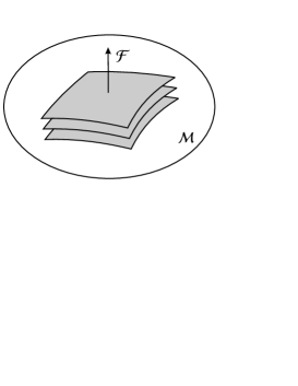
Figure 1: An example of a 3-dimensional moduli space $\mathcal{M}$ foliated by 2-dimensional symplectic sheets corresponding to a fixed value of a gauge field flux $\mathcal{F}$. On-shell quantization can determine symplectic structure on the sheets, but cannot be used to quantize the flux.

2.7 The role of dynamics

To get a nontrivial moduli space quantization, the symplectic form computed by the on-shell quantization method should be non-degenerate when restricted on $\mathcal{M}$. This implies that the canonical momenta should be nontrivial functions on $\mathcal{M}$, much like in the chiral boson example considered in Section 2.2, where we had $\pi=f^{\prime}(u)$. In the case of gravity this means that the class of solutions cannot be static. Indeed, for static solutions the extrinsic curvatures (12) are zero. Thus the canonical momenta (11) will be identically zero on $\mathcal{M}$, and the restricted symplectic form will vanish. This means that for static solutions, the parameters characterizing the moduli space do not acquire nontrivial commutators among themselves upon quantization.

The symplectic form will be usually non-degenerate if some dynamics is present. For example, the “Bubbling AdS” solutions considered in Section 3 below have nonzero angular momentum: they are stationary but not static, and this will be enough to make the symplectic form nondegenerate. The reason is that $N_{i}\neq 0$ in (12) and the extrinsic curvatures no longer vanish identically. In [5], the appearance of a nontrivial symplectic form on the moduli space was conjectured to be related to supersymmetry. However, it is easy to see that supersymmetry is neither necessary nor sufficient for that: the moduli spaces of cylindrical [25] or plane [26] gravitational waves have a nontrivial symplectic structure in pure gravity; on the other hand, the symplectic form will vanish on any moduli space of static supersymmetric solutions. Supersymmetry may be instrumental though to control corrections to the on-shell quantization results (see Sections 2.10) or to obtain simplified symplectic current expressions (see remarks at the end of Section 3.7.3).

The above remarks are useful in order to understand the relation of our method to the perhaps more familiar ‘moduli space approximation’ à la Manton [27, 28, 29, 30], where one usually starts with a moduli space describing multi-centered static black hole or soliton solutions. This moduli space is typically finite-dimensional, parametrized by the coordinates of the centers and possibly some extra parameters. For example, in the multi-centered extremal black hole case [30] the moduli space is $3n$-dimensional, where $n$ is the number of black holes. Then one considers slow scattering of these black holes (or solitons) and finds that it can be described by the geodesics in a certain (calculable) metric

$$ds^{2}=g_{ij}(q)dq^{i}dq^{j}\,.$$ (23)

Then one can consider quantization of this system of slowly moving solitons. But notice that in the process of introducing slow motion we enlarged the phase space by adjoining canonical momenta (corresponding to velocities). So, in the black hole case, the phase space becomes $6n$-dimensional, twice the dimensionality of the original moduli space. Also, in order to construct these slowly moving black hole solutions (and derive metric (23)), one should go off-shell, i.e. out of the original moduli space. If one were to recover the metric (23) using our method (which may or may not be possible in practice), one would have to compute the symplectic form on the extended $6n$-dimensional phase space. The symplectic form would be degenerate if restricted to the original $3n$-dimensional moduli space corresponding to the static configurations, in agreement with the above discussion. This means in particular that black hole center coordinates are not quantized by themselves.

2.8 On-shell quantization vs effective action

In essence, the on-shell quantization method does nothing but quantizing first-order fluctuations along the moduli space $\mathcal{M}$ (except that it provides a particularly efficient way to do this). This is particularly clear from the symplectic current expression (17), which involves only first-order perturbations of the fields and, moreover, depends only on the quadratic part of the Lagrangian as expanded around a given background. To see this explicitly, let us parametrize the fields $\phi^{A}$ in (17) by their deviations $\psi^{A}$ from a given background $\phi_{0}\in\mathcal{M}$:

$$\phi=\phi_{0}+\psi\,,$$ (24)

at the same time expanding the Lagrangian of the theory in terms of $\psi$:

$$L=\sum_{i=2}^{\infty}L^{(i)},$$ (25)

where $L^{(i)}$ is degree $i$ in $\psi$. The part linear in $\psi$ is absent, since we assume that $\phi_{0}$ is a solution. The coefficients of $L^{(i)}$ may and will generically depend on $\phi_{0}$, but the precise form of this dependence is irrelevant for our argument.

Now, as we showed in Section 2.5, the symplectic current is independent of the field choice. In particular, we can use $\psi^{A}$ to compute it. Thus we will have:

$$J_{CWZ}^{l}=\sum_{i=2}^{\infty}\delta\frac{\partial L^{(i)}}{\partial\partial_{l}\psi^{A}}\wedge\delta\psi^{A}.$$ (26)

Since $L^{(i)}$ is degree $i$ in $\psi,$ $\partial L^{(i)}/\partial\partial_{l}\psi$ will be degree ($i-1),$ and $\delta(\partial L^{(i)}/\partial\partial_{l}\psi)$ will be degree $(i-2)$ in $\psi$ (and linear in $\delta\psi$). So we see that once we evaluate (26) on shell by putting $\psi=0$, all the terms with $i\geq 3$ will vanish, and thus the symplectic current depends only on the quadratic part of the fluctuation Lagrangian.

This remark makes it clear that any result obtained by the on-shell quantization method can be in principle obtained by a more conventional method based on computing the quadratic action, quantizing it, and specializing to a particular subclass of perturbations corresponding to deformations along $\mathcal{M}$. In practice, however, there may be formidable difficulties in following the conventional path. The main difficulty is that the full quadratic action will typically have a complicated form, except around very special backgrounds. One could think that perhaps one could consider a truncation of the quadratic action to the fluctuation modes along $\mathcal{M}$, and that would have a chance to be simple. The problem here is that such a truncation does not even have to exist, since these modes can couple to other modes already on the quadratic level.

These difficulties are best demonstrated on a concrete example of the LLM family of solutions [4]. On-shell quantization of this family is considered in Section 3 below, and was also the subject of [2]. In this case the quadratic effective action is available around only one representative of the family, namely $AdS_{5}\times S^{5}$ [31, 32] (and can also be found around the plane wave, using the results of [33]). In any other case it is highly unlikely that a tractable quadratic action can be found. Moreover, even around $AdS_{5}\times S^{5}$ the quadratic action couples the moduli space modes characterized by the BPS condition $J=\Delta$ to the opposite angular momentum modes $J=-\Delta$, as a simple consequence of angular momentum conservation. This shows that on-shell quantization is the only practical way to quantize in the general case. However, around $AdS_{5}\times S^{5}$ both on-shell quantization and the quadratic effective action method can be applied, and the results agree as they should [2].

2.9 Hilbert space. Semiclassical states. Hamiltonian

Using the on-shell quantization method, we can compute the symplectic form on the moduli space of solutions. This symplectic form encodes the Poisson brackets between the functions defining the geometry (e.g. the shape of the droplets in the LLM case). Quantizing the brackets, we find commutation relations between these functions. We can then find a Hilbert space on which these functions are defined as operators so that the commutation relations are satisfied.

In principle, we will get a separate Hilbert space around each geometry from the moduli space. Low-lying states in this Hilbert space will not allow any semiclassical interpretation, they will be similar to states of a few field quanta (e.g. gravitons) propagating in Minkowski space. However, in the limit of large occupation numbers we can construct coherent states, which can be interpreted as describing a neighboring classical geometry. In this sense, neighboring geometries are contained in each other’s Hilbert spaces. This shows that all these Hilbert spaces will be isomorphic.

Let us now discuss the choice of a Hamiltonian operator on the Hilbert space. First of all, when we are dealing with a theory of gravity, it is by no means guaranteed that a preferred Hamiltonian will exist. For instance, this seems to be the situation for the plane gravitational wave case analyzed in [26]. For the concept of energy to make sense, all spacetimes in the considered moduli space must have a common asymptotic infinity with a timelike Killing vector. In this case the Hamiltonian can be defined by computing the classical energy of the considered solutions. For the LLM case, such a computation has been done in [4].

When a Hamiltonian is available, the process of quantization can be taken further by discussing the energy eigenstates. To avoid possible confusion we would like to stress again: the Hamiltonian is an independent piece of information which supplements the symplectic form computed by the on-shell quantization method. There are cases when it can be defined in the classical theory (and carried over to the quantum theory by the correspondence principle), but a separate computation is necessary in order to do that.

2.10 Corrections

In which sense does on-shell quantization approximate the true picture attainable in the complete theory? And what are the corrections which should be included if one is to go beyond this approximation? These are interesting questions, which most likely have to be analyzed on a case-by-case basis. Here we will limit ourselves to a few general remarks.

It will be convenient to phrase the discussion in the Hamiltonian language, which may not be the most general situation (see Section 2.9), but is sufficient for the applications we have in mind. The full Hamiltonian can be schematically represented as

$$H=H_{0}(\phi_{\|})+H_{0}(\phi_{\perp})+H_{\text{int}}\,.$$ (27)

Here $H_{0}(\phi_{\|})$ is the quadratic Hamiltonian for the fluctuation modes along the moduli space $\mathcal{M}$ (around a given background); $H_{0}(\phi_{\perp})$ is the quadratic Hamiltonian for the modes corresponding to fluctuations orthogonal to $\mathcal{M}$; $H_{\text{int}}$ is the interaction Hamiltonian.

On the quadratic level there is a complete decoupling between $\phi_{\|}$ and $\phi_{\perp}.$ It is only the $\phi_{\|}$ modes that we are quantizing using the on-shell quantization method, while $\phi_{\perp}$ are effectively frozen. The result of this quantization will be a Hilbert space $\mathcal{H}_{\|}$ and a spectrum of energy eigenstates.

It is more or less clear how this picture will have to be modified, if the corrections are to be considered. First of all, we will have to introduce a Hilbert space $\mathcal{H}_{\perp}$ for the orthogonal modes, with its own free spectrum. The full Hilbert space is then the direct product $\mathcal{H}_{\|}\otimes\mathcal{H}_{\perp}$. On-shell quantization can be thought of as turning off $H_{\text{int}}$ and putting all $\phi_{\perp}$ in their vacuum state, so that the full state is a product

$$|\phi_{\|}\rangle\otimes|0_{\perp}\rangle\,.$$ (28)

Taking $H_{\text{int}}$ into account allows transitions, exciting the orthogonal modes and inducing mixings between various states. To be able to treat $H_{\text{int}}$ as a perturbation, a small expansion parameter should be available. In this case the new energy eigenstates will be small perturbations of the original product states (28), with slightly shifted energy levels. In theories of gravity, the role of such an expansion parameter can be played by $\ell\Lambda_{\text{Planck}}$, the characteristic curvature radius $\ell$ of the background spacetime measured in Planck units. In the string theory context, this will correspond to the $\alpha^{\prime}$-expansion of the effective action.

In supersymmetric situations, the spectrum may be protected and energy shifts should not occur. For instance, we know from AdS/CFT that this should be the case for the LLM solutions. Indeed, the $\mathcal{N}=4$ SYM states dual to these geometries are 1/2 BPS, and their energies cannot depend on a continuous parameter. Notice that it would be wrong to conclude that the LLM geometries do not get modified once the $\alpha^{\prime}$-corrections are taken into account — they will, except in the fully supersymmetric cases of $AdS_{5}\times S^{5}$ and the plane wave. It is only the energy eigenstates which should remain protected. It would be interesting to show this directly from the gravity side.

The discussion of corrections becomes increasingly subtle when loop effects are taken into account. In the AdS/CFT context, the size of these effects is controlled by $1/N$. In this paper we mostly discuss the $N=\infty$ limit, corresponding to the classical SUGRA. In principle, it should be possible to consider $N\gg 1$ case as a perturbation over $N=\infty$. This would require inclusion of massive string states needed for the UV completion of the theory. In the LLM case, we know that this should lead to a reduction in the number of states with energies above $N$ (see Section 3.3). It would be extremely interesting to understand how such a reduction can be achieved in a perturbative treatment, and to reproduce it from the gravity side.

2.11 Summary of on-shell quantization method

To summarize, we have the following recipe for quantizing a moduli space of solutions of any supergravity theory. First of all, we have to find a general expression for the symplectic current of the theory. This is computed from the supergravity Lagrangian by the general formula (17) and will contain the Crnković-Witten gravitational symplectic current (15), as well as additional terms for the other fields of the theory.

Second, we have to evaluate the symplectic current on the moduli space of solutions. This is done by expressing the variations of all the fields in the symplectic current via the variations of the arbitrary functions describing the moduli space.

Finally, we have to integrate the symplectic current on a Cauchy surface $\Sigma$ to obtain the symplectic form, which will be a closed 2-form on the moduli space. This symplectic form can then be quantized in the standard way.

3 Quantization of “Bubbling AdS”

3.1 Supergravity solutions

Having set up the general framework in the previous section, we will now apply the on-shell quantization method to quantize the “Bubbling AdS” family of supergravity solutions found by LLM [4]. This family includes all regular 1/2 BPS solutions of Type IIB SUGRA with $SO(4)\times SO(4)\times\mathbb{R}$ symmetry. These solutions have constant dilaton and axion and vanishing 3-form. The metric has the form:

$$ds^{2}=-h^{-2}(dt+V_{i}dx^{i})^{2}+h^{2}(dy^{2}+dx^{i}dx^{i})+ye^{G}d\Omega_{3}^{2}+ye^{-G}d\tilde{\Omega}_{3}^{2}\,,$$ (29)

where $i=1,2$ , $d\Omega_{3}^{2}$ and $d\tilde{\Omega}_{3}^{2}$ are the metrics on two unit 3-spheres $S^{3},\tilde{S}^{3}.$ The functions $h$ and $G$ are determined in terms of a single function $z(x_{1},x_{2},y),$ $y>0$:

$$h^{-2}=\frac{y}{\sqrt{1/4-z^{2}}}\,,\qquad e^{2G}=\frac{1/2+z}{1/2-z}\,,$$ (30)

The $z$ and $V_{i}$ are in turn fixed in terms of one function $Z(x_{1},x_{2}),$ which can only take the values $\pm\frac{1}{2},$ and is also the boundary value of $z$ on the $y=0$ plane. Namely, we have:

$$z =\frac{1}{\pi}\frac{y^{2}}{(x^{2}+y^{2})^{2}}\ast Z\,,$$

$$V_{i} =\frac{\varepsilon^{ij}}{\pi}\frac{x_{j}}{(x^{2}+y^{2})^{2}}\ast Z\,.$$ (31)

Apart from the metric, only the 5-form is turned on:

$$F_{5} =F\wedge d\Omega_{3}+\tilde{F}\wedge d\tilde{\Omega}_{3}\,,$$

$$F =dB,\qquad\tilde{F}=d\tilde{B},\qquad$$ (32)

$d\Omega_{3},d\tilde{\Omega}_{3}$ being the volume forms of the spheres. The one-forms $B,\tilde{B}$ are defined up to a gauge transformation. A convenient choice is the axial gauge $B_{y}=\tilde{B}_{y}=0,$ the remaining components being then given by

$$B_{t} =-\frac{1}{4}y^{2}e^{2G}, \tilde{B}_{t} =-\frac{1}{4}y^{2}e^{-2G},$$ (33)

$$B_{i} =-\frac{y^{2}V_{i}}{4\left({\frac{1}{2}}-z\right)}-\frac{U_{i}}{4}-\frac{x_{1}}{4}\delta_{i,2}\,, \tilde{B}_{i} =-\frac{y^{2}V_{i}}{4\left({\frac{1}{2}}+z\right)}-\frac{U_{i}}{4}+\frac{x_{1}}{4}\delta_{i,2}\,$$ (34)

(see [2]), where

$$U_{i}\equiv\frac{\varepsilon^{ij}}{\pi}\frac{x_{j}}{x^{2}+y^{2}}\ast Z\,.$$ (35)

The following linear relations, evident from (31) and (35), will play an important role below:

$$\partial_{i}z =-y\,\varepsilon^{ij}\partial_{y}V_{j}\,,$$

$$\partial_{[i}V_{j]} \equiv\frac{1}{2}(\partial_{i}V_{j}-\partial_{j}V_{i})=\frac{1}{2y}\varepsilon_{ij}\partial_{y}z\,,$$ (36)

$$\partial_{y}U_{i} =-2yV_{i}\,.$$

3.2 Moduli space

The moduli space is parametrized by collections of droplets of arbitrary shape in the $x_{1},x_{2}$ plane, defined by the condition that $Z=-1/2$ on the union of all droplets (which we denote $\mathcal{D})$ and $Z=1/2$ in the remaining part of the plane, $\mathcal{D}^{c}$. We will assume that the boundaries of all droplets in $\mathcal{D}$ are smooth curves, so that the corresponding solution has a smooth geometry [4]. We would like to discuss the quantization of this moduli space. As discussed in Section 2, there are two aspects to the moduli space quantization. First we must detect all nontrivial fluxes. These can be quantized using an appropriate Dirac quantization condition. On the other hand, deformations within the moduli space corresponding to keeping all the fluxes fixed should be quantized using the on-shell quantization method.

The topology of the “Bubbling AdS” spacetimes and the corresponding fluxes have been already determined in [4]. It turns out that for every black or white region in the droplet plane there is a non-contractible 5-cycle supporting an $F_{5}$ flux proportional to the area of the corresponding region. For example, for each droplet (i.e. a black region) the corresponding 5-manifold is constructed by fibering the sphere $\tilde{S}^{3}$ over a surface $\Sigma_{2}$ capping the droplet as shown in Fig. 2. This 5-manifold is nonsingular, since the $\tilde{S}^{3}$ shrinks to zero size on the $y=0$ plane outside of the droplets in an appropriate way. Analogously, the 5-manifolds corresponding to the white regions are constructed by fibering the $S^{3}$ over surfaces capping these white ‘holes’ inside the droplets. Using flux quantization, one shows that the area of each black or white region must be quantized [4]:

$$A_{i}=\frac{\kappa_{10}}{2\pi^{3/2}}n_{i},\qquad n_{i}\in\mathbb{N}.$$ (37)

These integers can be thought of as the numbers of giant gravitons wrapping the $S^{3}$ and the $\tilde{S}^{3}$. The sum of $n_{i}$’s corresponding to the black regions should be equal $N,$ the total number of D3 branes making up the configuration.

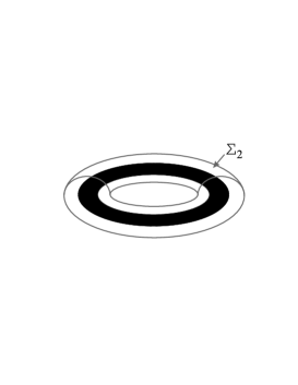
Figure 2: The surface $\Sigma_{2}$ caps the droplet in the $x_{1},x_{2}$ plane by extending into $y>0$. Fibering the $\tilde{S}^{3}$ over $\Sigma$, we get a closed 5-manifold supporting an $F_{5}$ flux proportional to the area of the droplet [4].

We see that there exists an infinite-dimensional class of deformations within the moduli space keeping all the fluxes fixed: these are precisely the deformations of the boundaries of the droplets which keep fixed the areas of all black and white regions. It is these deformations that we will quantize using the on-shell quantization method.

3.3 Dual description in terms of free fermions

The “Bubbling AdS” solutions corresponding to a collection of finite-size droplets are asymptotically $AdS_{5}\times S^{5}$. The AdS/CFT correspondence [1] can be used to relate these Type IIB supergravity solutions to states of the $\mathcal{N}=4$ supersymmetric Yang-Mills theory on $S^{3}\times\mathbb{R}$. Since the geometries are 1/2 BPS, the dual operators on the Yang-Mills side are chiral primaries with conformal weight equal to their $U(1)$ R-charge: $\Delta=J$. As is well known [7, 8], this sector of $\mathcal{N}=4$ super Yang-Mills admits a very simple description as a system of $N$ non-relativistic free fermions moving in a harmonic oscillator potential. In the large $N$ limit (which is what we are mostly concerned with in this paper) the states of the many-fermion system are well described as droplets in the one-particle phase space. In fact, these droplets are the same droplets which characterize the gravity solutions. For example, it was checked in [4] that the excitation energy of the “Bubbling AdS” solutions over $AdS_{5}\times S^{5}$ is equal to

$$\Delta=J=\frac{1}{4\pi\hbar^{2}}\left[\int_{\mathcal{D}}d^{2}x\,x^{2}-\frac{1}{2\pi}\left(\int_{\mathcal{D}}d^{2}x\right)^{2}\right]\,,$$ (38)

which is precisely the excitation energy of the fermionic state described by the droplet $\mathcal{D}$ over the ground state described by the circular droplet of the same area centered at the origin. The one-dimensional Planck constant $\hbar$ here can be fixed by comparing the area quantization condition (37) valid on the supergravity side with the semiclassical phase space quantization condition $A=2\pi\hbar n$, which should be true on the fermion side. This gives [4]:

$$\hbar=\frac{\kappa_{10}}{4\pi^{5/2}}\,.$$ (39)

In this paper we would like to compare the symplectic structures on the droplet space arising from the supergravity and the fermion side. On the supergravity side we will use the on-shell quantization method described in Section 2. On the fermion side the corresponding symplectic form can be found by using the so-called hydrodynamic approach, commonly used to describe edge states in Quantum Hall systems (see e.g. [35]). The idea of this method is to identify the one-fermion description of the classical dynamics of the droplets with the collective one. In the one-fermion picture, the droplet motion is described by solving the individual Hamilton equations

$$\dot{p}=-\partial_{q}H,\quad\dot{q}=\partial_{p}H,\quad H=\frac{p^{2}+q^{2}}{2\hbar}\,.$$ (40)

for the fermions localized close to the droplet boundary $\partial\mathcal{D}$. It is convenient to first look at the subclass of the droplets whose boundary curve can be described in polar coordinates as $r=r(\phi)$ for a single-valued function $r(\phi)$. For these droplets (40) implies that $r(\phi)$ evolves in time according to the classical chiral boson equation

$$\dot{r}=\hbar^{-1}r^{\prime}.$$ (41)

(A cautionary remark: as we will see below, it would be wrong to conclude from this that the in quantum theory $r(\phi)$ satisfies the chiral boson commutation relations.) In the collective pictures, one would like to recover the same equation (41) as a Hamilton equation of the form

$$\dot{r}=\{r,H_{\text{tot}}\}$$ (42)

where $H_{\text{tot}}$ is the total energy of the droplet state, given by the integral of the one-particle Hamiltonian:

$$H_{\text{tot}} =\int_{\mathcal{D}}\frac{dp\,dq}{2\pi\hbar}\frac{p^{2}+q^{2}}{2\hbar}$$

$$=\,\frac{1}{16\pi\hbar^{2}}\oint_{\partial\mathcal{D}}d\phi\,r^{4}(\phi),$$ (43)

while the Poisson bracket $\{,\}$ is to be determined from consistency of the two pictures. As we showed in [2] (see also [36], and especially [37], Eq. (4.3)), the appropriate Poisson bracket which generates the correct equation is

$$\{r^{2}(\phi),r^{2}(\tilde{\phi})\}=8\pi\hbar\,\delta^{\prime}(\phi-\tilde{\phi}).$$ (44)

The symplectic form corresponding to these Poisson brackets can be written as:

$$\omega_{\text{ferm}}=\frac{1}{32\pi\hbar}\oint\oint d\phi\,d\tilde{\phi}\,\text{Sign}(\phi-\tilde{\phi})\,\delta\left[r^{2}(\phi)\right]\wedge\delta\left[r^{2}(\tilde{\phi})\right]\,.$$ (45)

The total area of the droplet is proportional to the total number of fermions and must be kept fixed. This means that the variations in (45) must satisfy the constraint

$$\oint d\phi\,\,\delta\left[r^{2}(\phi)\right]=0\,.$$ (46)

Under this constraint, the symplectic form (45) is well defined as written, in spite of the fact that the kernel Sign$(\phi-\tilde{\phi})$ is not periodic. In fact we can add to the kernel any function of the form $g_{1}(\phi)+g_{2}(\tilde{\phi})$ without changing the answer. If desired, one can consider adding $(\tilde{\phi}-\phi)/\pi$, which will make the kernel explicitly periodic.

It is interesting to note that although the symplectic form (45) is easiest to derive for the particular case of the harmonic oscillator one-fermion Hamiltonian, it is in fact completely general and will describe the motion of droplets of noninteracting fermions described by an arbitrary one-particle Hamiltonian $H(p,q)$ [36],[2],[37].

Let us rewrite (45) in a slightly different form, introducing instead of $\phi$ a natural parameter $s$ measuring arc length along $\partial\mathcal{D}$. From elementary geometry we have

$$\frac{ds}{r(\phi)d\phi}=\frac{\delta r}{\delta\gamma_{\perp}}\,,$$ (47)

where by $\delta\gamma_{\perp}$ we denote the variation of $\partial\mathcal{D}$ in the outside normal direction. Thus (45) can be equivalently written as

$$\omega_{\text{ferm}}=\frac{1}{8\pi\hbar}\oint\oint ds\,d\tilde{s}\,\text{Sign}(s-\tilde{s})\,\delta\gamma_{\perp}(s)\wedge\delta\gamma_{\perp}(\tilde{s})\,.$$ (48)

The constraint (46) takes the form

$$\oint ds\,\delta\gamma_{\perp}(s)=0\,.$$ (49)

The advantage of expression (48) is that it is completely general — it makes no reference to polar coordinates and can be also used for droplets with multiple-valued $r(\phi)$. It is this expression that we will have to reproduce from the supergravity side.

The Poisson bracket following from (48),

$$\{\delta\gamma_{\perp}(s),\delta\gamma_{\perp}(\tilde{s})\}=2\pi\hbar\,\delta^{\prime}(s-\tilde{s})\,,$$ (50)

is equivalent to the bracket derived by Dhar [37], Eq. (4.2), using a reparametrization-invariant description of fermion droplet boundaries. In Appendix A.1 we show explicitly that (50) generates correct equations of motion of droplet boundary in the general case.

A few words should be said about the symplectic structure in the situation when several droplets are present, or when a single droplet has several boundary components. Assume that $\partial\mathcal{D}$ has $B$ connected components described by closed curves $\gamma^{(b)}(s)$. In this case one has to introduce a separate field $\,\delta\gamma_{\perp}^{(b)}(s)$ for each boundary. The total symplectic form is given by the sum of the forms (48) computed for each boundary component:

$$\omega_{\text{ferm}}=\frac{1}{8\pi\hbar}\sum_{b=1}^{B}\oint\oint_{\gamma^{(b)}}ds\,d\tilde{s}\,\text{Sign}(s-\tilde{s})\,\delta\gamma_{\perp}^{(b)}(s)\wedge\delta\gamma_{\perp}^{(b)}(\tilde{s})\,.$$ (51)

Each $\delta\gamma_{\perp}^{(b)}(s)$ has to satisfy its own constraint

$$\oint_{\gamma^{(b)}}\delta\gamma_{\perp}^{(b)}(s)\,ds=0\,.$$ (52)

This means that, semiclassically, different droplet boundaries are completely decoupled, and it is impossible for a fermion to move from one boundary to another, even though such a transition would keep the total area of the droplet fixed. Technically, condition (52) specifies symplectic sheets in the moduli space of fermion droplets.

The symplectic form (51) on variations satisfying (52) is all we need for future comparison with the supergravity side, since as we discussed in the previous subsection, only variations keeping both black and white areas fixed can be quantized by the on-shell quantization method, due to the fixed flux restriction.

Knowing the Poisson brackets, it is trivial to quantize the system. We will do this around the circular droplet, the general case being identical. We start by expanding $r^{2}(\phi)$ in Fourier series:

$$r^{2}(\phi)=\sum\alpha_{n}e^{in\phi},\qquad\alpha_{-n}=\alpha_{n}^{\ast}.$$ (53)

The zero mode is fixed in terms of the droplet area:

$$\alpha_{0}=\frac{A}{\pi}.$$ (54)

The $n\neq 0$ modes correspond to the area-preserving deformations. Substituting (53) in (45), we get Poisson brackets in terms of the corresponding Fourier coefficients:

$$\{\alpha_{n},\alpha_{m}\}=-4\hbar in\delta_{n+m}\,,$$ (55)

which upon quantization become commutators:

$$[\alpha_{n},\alpha_{m}]=4\hbar^{2}n\delta_{n+m}\,,$$ (56)

The Hilbert space of the theory can be constructed as a bosonic Fock space with $\alpha_{n},$ $n>0$ $(n<0)$ as annihilation (creation) operators. The Hamiltonian can be expressed in terms of these operators as

$$H=\frac{1}{4\hbar^{2}}\sum_{n>0}\alpha_{-n}\alpha_{n}+\text{Const.}$$ (57)

It is interesting to compare the partition function of this theory

$$Z(\beta)=\prod_{n=1}^{\infty}\frac{1}{1-e^{-\beta n}}\,.$$ (58)

with the exact partition function for a system of $N<\infty$ fermions in the harmonic oscillator potential:

$$Z_{N}(\beta)=\prod_{n=1}^{N}\frac{1}{1-e^{-\beta n}}\,.$$ (59)

Writing the partition functions in the form

$$Z(\beta)=\sum_{E_{i}}g(E_{i})e^{-\beta E_{i}}\,,$$ (60)

we can read off the degeneracy $g(E_{i})$ of the energy state $E_{i}$. We see that the infinite $N$ computation correctly predicts the finite $N$ energy levels $E_{i}=1,2,3,\ldots$ However, it reproduces their degeneracies only up to energies $E_{i}\leq N,$ overestimating the degeneracy of higher energy levels.

3.4 Symplectic form of Type IIB SUGRA

The LLM solutions satisfy the equations of motion that can be derived from the following consistent truncation of the Type IIB SUGRA action:

$$S=\frac{1}{2\kappa_{10}^{2}}\int d^{10}x\sqrt{-g}\left(R-4F_{|i_{1}\ldots i_{5}|}F^{|i_{1}\ldots i_{5}|}\right),$$ (61)

We can proceed using this action if we impose the selfduality constraint $F_{5}=\ast F_{5}$ on the solutions. The presence of this constraint does not modify the underlying symplectic form of the theory, which can be computed from the action (61).

Using the general formulas from Section 2, the symplectic form will be equal to

$$\omega=\frac{1}{2\kappa_{10}^{2}}\int d\Sigma_{l}(J_{G}^{l}+J_{F}^{l}),$$ (62)

where $J_{G}^{l}$ and $J_{F}^{l}$ are symplectic currents constructed from the gravity and 5-form parts of the Langrangian using (17). In fact $J_{G}^{l}$ is nothing but the Crnković-Witten current (15). To find the 5-form current, we take the potentials $A_{|k_{1}\ldots k_{4}|}$ $(F_{5}=dA)$ as our basic fields. Applying (17), we get immediately

$$J_{F}^{l}=-8\,\delta(\sqrt{-g}F^{l|k_{1}\ldots k_{4}|})\,\wedge\delta A_{|k_{1}\ldots k_{4}|}.$$ (63)

Now that we computed the symplectic current, we can simplify it using the selfduality constraint, which can be written as

$$\sqrt{-g}F^{l_{1}\ldots l_{5}}=\varepsilon^{l_{1}\ldots l_{5}|m_{1}\ldots m_{5}|}F_{|m_{1}\ldots m_{5}|},$$ (64)

where $\varepsilon^{\ldots}$ is the flat 10-dimensional epsilon symbol. Thus we have

$$J_{F}^{l}=-8\,\varepsilon^{l|k_{1}\ldots k_{4}||m_{1}\ldots m_{5}|}\delta F_{|m_{1}\ldots m_{5}|}\wedge\delta A_{|k_{1}\ldots k_{4}|}.$$ (65)

3.5 Regularity condition. Boundary term

To evaluate the symplectic form, we will use $\Sigma=\{t=const\}$ in (14). This is a natural choice, in view of the time-independence of the solutions. With this choice, $J^{t}$ is the only needed component of the symplectic current. Because of the $SO(4)\times SO(4)$ symmetry, integration over the 3-spheres is trivial, and we will have

$$\omega=\frac{(2\pi^{2})^{2}}{2\kappa_{10}^{2}}\int dy\,d^{2}x(J_{G}^{t}+J_{F}^{t})\,.$$ (66)

There is however a subtlety to be discussed, before we start evaluating this integral. Namely, we have to make sure that the field perturbations we are using are regular. More precisely, this condition means that $\delta g_{mn}$ and $\delta A_{4}$ should be regular in a local coordinate system in which the background metric $g_{mn}$ is regular (such a coordinate system exists because all LLM geometries are regular). If this condition is violated, we may get a wrong result for the symplectic form. In fact, as we will explain below, this was precisely the origin of the factor 1/2 discrepancy encountered in [2]. The source of trouble is $\delta A_{4},$ which has the form

$$\delta A_{4}=\delta B\wedge d\Omega+\delta\tilde{B}\wedge d\tilde{\Omega}\,$$ (67)

and does not satisfy the regularity condition on the $y=0$ plane if the axial gauge expressions (34) are used. In fact, $\delta B$ and $\delta\tilde{B}$ obtained by perturbing (34) tend to a finite nonzero limit as $y\rightarrow 0$. On the other hand, the spheres $S^{3}(\tilde{S}^{3})$, whose volume forms appear in (67), shrink to zero size inside (outside) the droplets. This means that the four-form (67) is singular as $y\rightarrow 0$.

To get the right answer for the symplectic form, we must use in (65) a regular gauge field perturbation $\delta A_{4}^{\text{reg}}$. The existence of such a regular perturbation and its properties are discussed in detail in Appendix A.2. The result of this analysis is that $\delta A_{4}^{\text{reg}}$ can be chosen to have the form

$$\delta A_{4}^{\text{reg}}=\delta B^{\text{reg}}\wedge d\Omega+\delta\tilde{B}^{\text{reg}}\wedge d\tilde{\Omega}\,,$$ (68)

where $\delta B^{\text{reg}},\delta\tilde{B}^{\text{reg}}$ are regular functions at $y\geq 0$, which have zero $y=0$ limits on $\mathcal{D}$($\mathcal{D}^{c}$) as a consequence of the regularity of $\delta A_{4}^{\text{reg}}$:

$$\delta B^{\text{reg}}|_{y=0} = 0\quad\text{on }\mathcal{D},$$

$$\delta\tilde{B}^{\text{reg}}|_{y=0} = 0\quad\text{on }\mathcal{D}^{c}.$$ (69)

(the precise regularity condition is somewhat stronger, see appendix A.2).

Since $\delta A_{4}^{\text{reg}}$ must be related to $\delta A_{4}$ by a gauge transformation, we must have

$$\delta B^{\text{reg}}=\delta B-d\lambda\,,\qquad\delta\tilde{B}^{\text{reg}}=\delta\tilde{B}-d\tilde{\lambda}\,$$ (70)

for some regular functions $\lambda,\tilde{\lambda}$.

Now we are ready to find the 5-form part of the symplectic form. First of all, substituting (68) into (65), we get

$$J_{F}^{t}=4\varepsilon^{abc}(\,\delta B_{a}^{\text{reg}}\wedge\delta\tilde{F}_{bc}-\delta\tilde{B}_{a}^{\text{reg}}\wedge\delta F_{bc}\,)\,\,.$$ (71)

Using (70), this can be expressed as

$$J_{F}^{t} =4\varepsilon^{abc}(\,\delta B_{a}\wedge\delta\tilde{F}_{bc}-\delta\tilde{B}_{a}\wedge\delta F_{bc}\,)\,-4\varepsilon^{abc}(\,\partial_{a}\lambda\wedge\delta\tilde{F}_{bc}-\partial_{a}\tilde{\lambda}\wedge\delta F_{bc}\,)\,$$

$$=8\varepsilon^{ij}(\partial_{y}\delta B_{i}\,\wedge\delta\tilde{B}_{j}-\delta B_{i}\,\wedge\partial_{y}\delta\tilde{B}_{j})-4\varepsilon^{abc}\partial_{a}(\,\lambda\wedge\delta\tilde{F}_{bc}-\tilde{\lambda}\wedge\delta F_{bc}\,)\,\,,$$ (72)

where we simplified the first term using the axial gauge condition $B_{y}=\tilde{B}_{y}=0$ and used the closedness of $F$ and $\tilde{F}$ to rewrite the second term as a total derivative. Contribution of this term to the integral in (66) will be given by a boundary term at $y=0$. More precisely, we will have

$$\int dy\,d^{2}x\,J_{F}^{t}\,=\int dy\,d^{2}x\,J_{F}^{\text{bulk}}+\int_{y=0}d^{2}x\,J_{F}^{\text{bdry}}\,,$$ (73)

where

$$J_{F}^{\text{bulk}} =8\,\varepsilon^{ij}(\partial_{y}\delta B_{i}\,\wedge\delta\tilde{B}_{j}-\delta B_{i}\,\wedge\partial_{y}\delta\tilde{B}_{j})\,,$$

$$J_{F}^{\text{bdry}} =8\,(\lambda\wedge\delta\tilde{F}_{12}-\tilde{\lambda}\wedge\delta F_{12}\,)\,\,.$$ (74)

If we had used the singular perturbation $\delta A_{4}$ in (65), we would have missed the boundary term in (73). This is what caused the factor 1/2 discrepancy encountered in Section 6 of [2].

Eq. (73) is the final general expression for the 5-form part of the symplectic form. We see that to evaluate it, we only need to know the functions $\lambda$ ($\tilde{\lambda}$) at $y=0$. Their values on $\mathcal{D}$ ($\mathcal{D}^{c}$) can be determined from (69). Using (70), we see that we must solve the equations

$$\delta B_{i} =\partial_{i}\lambda\quad\text{on }\mathcal{D},$$

$$\delta\tilde{B}_{i} =\partial_{i}\tilde{\lambda}\quad\text{on }\mathcal{D}^{c}.$$ (75)

In the complementary regions $\lambda$ ($\tilde{\lambda}$) can be defined arbitrarily, since the field strengths multiplying these functions in $J_{F}^{\text{bdry}}$ will vanish there as a consequence of (75). This is of course not surprising, since making $\lambda$ or $\tilde{\lambda}$ nonzero in the complementary regions corresponds to a perfectly regular gauge transformation.

Let us repeat the logic of the preceding discussion. We observed that the axial-gauge perturbation $\delta A_{4}$ is singular at $y=0.$ We must therefore gauge-transform $\delta A_{4}$ into a regular perturbation $\delta A_{4}^{\text{reg}}$. Such a regular form must exist, since all the fluxes are kept fixed. In principle, it is $\delta A_{4}^{\text{reg}}$ which should be used to compute the symplectic form. However, in practice it would be convenient to be able to use the explicit axial gauge expressions. Eq. (73) shows that we can keep using $\delta A_{4}$ to compute the symplectic current, but we have to pay a small price of adding a term to the symplectic form localized on the lower-dimensional submanifold where $\delta A_{4}$ becomes singular, i.e. at $y=0$. We will refer to this term as the boundary term, although of course it should be remembered that $y=0$ is only a coordinate boundary and the spacetime is completely regular there.

It remains to discuss the regularity of $\delta g_{mn}$. This perturbation is manifestly regular everywhere at $y=0$ except maybe at $\partial\mathcal{D}$. Thus we see that the situation is better than with $\delta A_{4},$ already because the singularity occurs on a smaller set. In fact, one can show that the remaining singularity on $\partial\mathcal{D}$ is harmless, and does not give rise to any additional terms in the symplectic form. The argument, which we will not present here in detail, proceeds by constructing a linear gauge transformation which completely removes the singularity in $\delta g_{mn},$ and by showing that this gauge transformation has no effect on the symplectic form. Thus the gravitational part of the symplectic form can be computed by using the naive expressions for $\delta g_{mn}$ in the Crnković-Witten symplectic current (15).

3.6 Wavy line approximation

We will now use our method to compute the symplectic form around the plane wave background, described by the droplet filling the lower half-plane: $\mathcal{D}=\{x_{2}<0\}$. The fluctuations around this background correspond to deforming $\partial\mathcal{D}$ from $x_{2}=0$ into $x_{2}=\varepsilon(x_{1}).$ The symplectic form will be an antisymmetric bilinear functional of $\varepsilon(x)$. The most general form of such a functional is

$$\omega=\int\int dx\,d\tilde{x}\,K(x,\tilde{x})\,\varepsilon(x)\wedge\varepsilon(\tilde{x})\,,\quad K(\tilde{x},x)=-K(x,\tilde{x})\,.$$ (76)

Since $x_{1}\rightarrow x_{1}+const$ is a symmetry of the plane wave background, the kernel $K(x,\tilde{x})$ will be translationally invariant: $K(x,\tilde{x})=K(x-\tilde{x})$. This suggests that we should work in the Fourier-transformed basis, in which $\omega$ will have a diagonal form:

$$\omega= \int\frac{dp}{2\pi}\,K(p)\,\varepsilon(p)\wedge\varepsilon(-p),\quad K(p)=K(-p),$$ (77)

$$\varepsilon(p)\equiv\int dx\,e^{ipx}\varepsilon(x).$$ (78)

We will now determine the precise form of $K$ by an explicit computation.

3.6.1 Gravitational part

In this subsection we will evaluate the gravitational part of the symplectic form, which is given by the integral of the Crnković-Witten current (15). It should be stressed that splitting the full symplectic form into the ‘gravitational part’ and ‘five-form part’ has no physical meaning; in particular, these parts will not be separately invariant under gauge transformations or changes of $\Sigma$. It is done here for purely computational purposes.

The background values of the fields characterizing the plane wave metric are found from (31) for $Z=\frac{1}{2}\text{Sign}\,x_{2}$ and are given by ($r\equiv\sqrt{x_{2}^{2}+y^{2}}$)

$$z=\frac{x_{2}}{2r}\,,\quad V_{1}=-\frac{1}{2r},\quad V_{2}=0\,.$$ (79)

To find the perturbations of these fields, we have to expand (31) to the first order in $\varepsilon(x)$. As we noted above, it is natural to Fourier-transform w.r.t. $x_{1}$. In this basis, the perturbations have the following form [2]:

$$\delta z(p) =-y^{2}\frac{1+r|p|}{2r^{3}}e^{-r|p|}\varepsilon(p)\,,$$

$$\delta V_{1}(p) =-x_{2}\frac{1+r|p|}{2r^{3}}e^{-r|p|}\varepsilon(p)\,,$$

$$\delta V_{2}(p) =\frac{ip}{2r}e^{-r|p|}\varepsilon(p)\,,$$ (80)

where

$$\delta z(p)\equiv\delta z(p,x_{2},y)\equiv\int dx_{1}\,e^{ipx_{1}}\delta z(x_{1},x_{2},y),\quad\text{etc}.$$

To find perturbations of the metric components one should also vary Eqs. (30) and use the above $\delta z$. We do not present the results of these elementary computations here.

According to (66), we have to compute the time-component of the Crnković-Witten current (15). The computation is straightforward. The current is a bilinear expression in $\varepsilon(p_{i})$, $i=1,2$. Here we present the result of integrating this expression in $x_{1}$, which produces a momentum-conserving $\delta$-function $p_{1}+p_{2}=0$:

$$\int dx_{1}J_{G}^{t}=\int\frac{dp}{2\pi}\left[2r^{2}p^{2}+2r|p|-1+\left(2r^{2}p^{2}+4r|p|+3\right)\frac{x_{2}^{2}}{r^{2}}\right]\frac{ipy^{3}}{2r^{3}}e^{-2r|p|}\varepsilon(p)\wedge\varepsilon(-p)\,.$$ (81)

This expression still has to be integrated in $y>0$ and $x_{2}$. The dependence on $p$ can be scaled out of the integrand by making the change of variables $r\rightarrow r/|p|$. The remaining integral is easy to evaluate in polar coordinates, and the final result is:

$$\int dx_{1}\,dx_{2}\,dy\,J_{G}^{t}=\int\frac{dp}{2\pi}\frac{i}{p}\varepsilon(p)\wedge\varepsilon(-p)\,.$$ (82)

This result was also derived in [2] by using the general expressions for the symplectic current, which we will present in Section 3.7.1 below.

3.6.2 Five-form part

Perturbations of the gauge field potentials can be analogously found from (34) [2]:

$$\delta B_{1}(p) =-\frac{1}{4}e^{-r|p|}\,\left[x_{2}|p|+(1+|p|r)\right]\varepsilon(p)\,,$$

$$\delta\tilde{B}_{1}(p) =-\frac{1}{4}e^{-r|p|}\,\left[x_{2}|p|-(1+|p|r)\right]\varepsilon(p)\,,$$ (83)

$$\delta B_{2}(p)=(i\,\text{Sign\thinspace}p)\,\delta B_{1}(p)\,,\qquad\delta\tilde{B}_{2}(p)=-(i\,\text{Sign\thinspace}p)\,\delta B_{1}(p)\,.$$ (84)

As we found in [2], the bulk term in the gauge field symplectic form expression (73) vanishes on these perturbations:

$$\int d^{2}x\,dy\,J_{F}^{\text{bulk}}=0\qquad\text{(plane wave)\thinspace.}$$ (85)

Thus the only contribution will come from the boundary term in (74). The field strengths at $y=0$ are easily found to be

$$\delta F_{12}(p) =-p^{2}x_{2}e^{-x_{2}|p|}\varepsilon(p)\qquad(x_{2}>0),$$

$$\delta\tilde{F}_{12}(p) =p^{2}x_{2}e^{x_{2}|p|}\varepsilon(p)\qquad(x_{2}<0).$$ (86)

The field strength variations vanish in the regions complementary to the given, and thus the corresponding variations of the potentials are pure gauge, in agreement with our discussion in Section 3.5. Solving (75), we find the gauge transformation parameters:

$$\lambda(p) =-\frac{i}{4p}e^{x_{2}|p|}\varepsilon(p)\,\qquad(x_{2}<0),$$

$$\tilde{\lambda}(p) =\frac{i}{4p}e^{-x_{2}|p|}\varepsilon(p)\,\qquad(x_{2}>0).$$ (87)

With this information it is possible to evaluate the boundary term in (73):

$$\int_{y=0}d^{2}x\,J_{F}^{\text{bdry}}\,=8\int_{y=0,x_{2}<0}\,\lambda\wedge\delta\tilde{F}_{12}-8\int_{y=0,x_{2}>0}\,\tilde{\lambda}\wedge\delta F_{12}\,=\,\int\frac{dp}{2\pi}\frac{i}{p}\varepsilon(p)\wedge\varepsilon(-p)\,\,.$$ (88)

3.6.3 Plane wave symplectic form

Adding the contributions of (82) and (88) in (66), we get the symplectic form for perturbations around the plane wave background:

$$\omega=\frac{4\pi^{4}}{\kappa_{10}^{2}}\int\frac{dp}{2\pi}\frac{i}{p}\,\varepsilon(p)\wedge\varepsilon(-p).$$ (89)

Since $i/p$ is the Fourier transform of $\frac{1}{2}$Sign$x$, this can be rewritten in the coordinate space as

$$\omega=\frac{2\pi^{4}}{\kappa_{10}^{2}}\int\int dx\,d\tilde{x}\,\text{Sign}(x-\tilde{x})\,\varepsilon(x)\wedge\varepsilon(\tilde{x}).$$ (90)

We would now like to compare this answer with the fermion symplectic form $\omega_{\text{ferm}}$ given by (45). These symplectic forms encode Poisson brackets between different Fourier harmonics of the boundary curve perturbation $\gamma_{\perp}(s)\equiv\varepsilon(x)$. Strictly speaking, we must compare commutation relations, which differ from the Poisson brackets by an extra Planck constant factor, $\hbar_{10}$ on the supergravity side and $\hbar$ on the fermion side. Since the 10-dimensional Planck constant satisfies the usual convention $\hbar_{10}=1,$ the precise relation which should be satisfied is

$$\omega=\hbar^{-1}\omega_{\text{ferm}}\,.$$ (91)

Using the value of $\hbar$ from (39), we see that this is indeed true.

3.7 General droplet case

In this section we will compute the symplectic form on the full moduli space.

3.7.1 Current expressions

The first step is to evaluate the symplectic current as a function of variations of the various fields describing the solutions. The gravitational part of the symplectic current was evaluated in [2] and is given by

$$J_{G}^{t}=~{}y^{3}\biggl{[}-\frac{1}{4}\delta(V_{i}\partial_{i}h^{-4})\wedge\delta(h^{4})+3\delta(V_{i}\partial_{i}G)\wedge\delta G +2\delta(h^{-4}V_{j}\,\partial_{[i}V_{j]})\wedge\delta V_{i}$$

$$-4\delta(\partial_{i}\ln h)\wedge\delta V_{i}\biggr{]}\,.$$ (92)

The last term can be represented as a total derivative by using $\partial_{i}V_{i}=0$. In the remaining terms we express $h$ and $G$ via $z$ from (30). We also choose to use the linear relations (36) to eliminate $\partial_{i}z$ and $\partial_{[i}V_{j]}$ in favor of $\partial_{y}V_{i}$ and $\partial_{y}z$. The resulting simplified expression has the form:

$$J_{G}^{t}=~{}{\frac{y^{4}\left(\frac{3}{4}+z^{2}\right)}{\left(\frac{1}{4}-z^{2}\right)^{2}}\varepsilon_{ij}\,}\delta(V_{j}\,\partial_{y}V_{i})\wedge\delta z-y^{4}\varepsilon_{ij}\,\delta\left({\frac{V_{i}\,\partial_{y}z}{\frac{1}{4}-z^{2}}}\right)\wedge\delta V_{j}-4\partial_{i}\left(\delta\ln h\wedge\delta V_{i}\right)\,.$$ (93)

To compute the five-form symplectic current, it is convenient to rewrite the gauge potential perturbations (34) in the form

$$\delta B_{i} =-\frac{1}{4}(a_{i}+b_{i}),\quad\delta\tilde{B}_{i}=-\frac{1}{4}(a_{i}-b_{i}),$$

$$a_{i} \equiv\delta\left[\frac{y^{2}V_{i}}{2\left({\frac{1}{4}}-z^{2}\right)}+U_{i}\right]\,,$$ (94)

$$b_{i} \equiv\delta\left[\frac{y^{2}z\,V_{i}}{{\frac{1}{4}}-z^{2}}\right]\,.$$

The bulk integrand in (73) then takes the form:

$$J_{F}^{\text{bulk}} =\varepsilon_{ij}(a_{i}\wedge\partial_{y}b_{j}-\partial_{y}a_{i}\wedge b_{j})\,$$

$$=-2\varepsilon_{ij}\,\partial_{y}a_{i}\wedge b_{j}\,+\partial_{y}\left(\varepsilon_{ij}a_{i}\wedge b_{j}\right)\,$$

$$=-2\varepsilon_{ij}\,\delta\left[\partial_{y}\frac{y^{2}V_{i}}{2\left({\frac{1}{4}}-z^{2}\right)}-2yV_{i}\right]\wedge\delta\left[\frac{y^{2}z\,V_{j}}{{\frac{1}{4}}-z^{2}}\right]+\partial_{y}\left(\varepsilon_{ij}a_{i}\wedge b_{j}\right)\,,\,$$ (95)

where we used (36) to express $\partial_{y}U_{i}$ via $V_{i}$ in the first term of this expression, so that it became a function of $V_{i}$ and $z$ only.

3.7.2 Total derivative representation

To find the symplectic form, we will have to integrate the bulk currents $J_{G}^{t}$ and $J_{F}^{\text{bulk}}$ found in the previous section. We see that these currents are given by complicated nonlinear expressions, so that performing this integration seems to be a daunting task. Our only hope to do the integral is to look for a total derivative representation of the total bulk current:

$$J^{\text{bulk}}\equiv J_{G}^{t}+J_{F}^{\text{bulk}}\overset{?}{=}\partial_{y}I^{y}+\partial_{i}I^{i}\,.$$ (96)

If such a representation exists, then the bulk integral will localize to the (coordinate) boundary and will be computable.

As we will explain now, there is a systematic way to look for representations of this kind. First of all, notice that the last terms of (93) and (95) already have the required total derivative form. Let $\tilde{J}^{\text{bulk}}$ denote the sum of the remaining terms. We can expand $\tilde{J}^{\text{bulk}}$ in the basis of 2-forms built out of $\delta z$, $\delta V_{i}$ and their $y$-derivatives:

$$\tilde{J}^{\text{bulk}}=A\epsilon_{ij}\delta V_{i}\wedge\delta V_{j}+B\epsilon_{ij}\partial_{y}\delta V_{i}\wedge\delta V_{j}+M_{i}\delta V_{i}\wedge\partial_{y}\delta z+N_{i}\partial_{y}\delta V_{i}\wedge\delta z\,+P_{i}\delta V_{i}\wedge\delta z.$$ (97)

The coefficients in this expansion are easy to find from (93), (95), and we won’t present them here.

Now we consider the following ansatz:

$$\tilde{J}^{\text{bulk}} =\partial_{y}\tilde{I}^{y}+\partial_{i}\tilde{I}^{i}\,,$$

$$\tilde{I}^{y} =\alpha\,\varepsilon_{ij}\delta V_{i}\wedge\delta V_{j}+\beta_{i}\,\delta V_{i}\wedge\delta z\,,$$ (98)

$$\tilde{I}^{i} =F\,\delta V_{i}\wedge\delta z\,.$$

This ansatz is natural if we assume that $\tilde{I}^{a}$ is given by local expressions in field variations. Since $\tilde{I}^{a}$ should contain one derivative less than $\tilde{J}^{\text{bulk}},$ it should be built entirely from $\delta z$ and $\delta V_{i}$. Comparing the coefficients, we get the following set of equations:

$$A =\partial_{y}\alpha$$

$$B =2\alpha-yF$$

$$M_{i} =N_{i}=\beta_{i}$$

$$P_{i} =\partial_{y}\beta_{i}+\partial_{i}F$$ (99)

(to get the second equation, one has to express $\partial_{i}z$ via $\partial_{y}V_{i}$ using (36)). It turns out that these equations indeed admit a solution. Namely, from the first three equations one finds:

$$\alpha =-\frac{y^{4}z\left(\frac{1}{4}+z^{2}\right)}{\left(\frac{1}{4}-z^{2}\right)^{2}}\,,$$

$$\beta_{i} =-{\frac{y^{4}\epsilon_{ij}V_{j}}{\frac{1}{4}-z^{2}}-\frac{2y^{4}z^{2}\varepsilon_{ij}V_{j}}{\left(\frac{1}{4}-z^{2}\right)^{3}}\,,}$$ (100)

$$F =\frac{2y^{3}z}{\frac{1}{4}-z^{2}}\,.$$

One then can check, using (36), that the remaining fourth equation is also satisfied, and thus we have constructed a total derivative representation for $\tilde{J}^{\text{bulk}}$. The total derivative representation for $J^{\text{bulk}}$ follows when we take the last terms in (93) and (95) into account:

$$J^{\text{bulk}} =\partial_{y}I^{y}+\partial_{i}I^{i}\,,$$

$$I^{y} =\varepsilon_{ij}\delta V_{i}\wedge\delta(\alpha V_{j})+\varepsilon_{ij}a_{i}\wedge b_{j}\,,$$ (101)

$$I^{i} =F\,\delta V_{i}\wedge\delta z\,-4\delta\ln h\wedge\delta V_{i}\,.$$

Here it was possible to simplify the $I^{y}$ by noticing that the found coefficients $\alpha$ and $\beta_{i}$ are in fact related by

$$\beta_{i}=\frac{\partial\alpha}{\partial z}\varepsilon_{ij}V_{j}\,.$$ (102)

We end this subsection with the following remark. One could think that since the symplectic current is conserved, it can always be represented as a total derivative, i.e. we will always have

$$\ast J=d\Theta\,.$$ (103)

This is of course true, at least locally. But there is a crucial point, which makes looking for a representation of this kind rather useless in general. Namely, while $J$ of course is given by an expression which is local in the variations of the fields, $\Theta$ in general will be non-local. For instance, in the chiral boson example considered in Section 2.2, the symplectic current restricted to the chiral boson moduli space has the form

$$J^{v}=\delta f^{\prime}(u)\wedge\delta f(u)\,.$$ (104)

It is obvious that this cannot be represented as a $u$-derivative of an expression local in $\delta f$.

It is thus clear that something special is going on in our case, since we did find a total derivative representation local in the variations of the fields. It would be extremely interesting to provide an explanation for this phenomenon, and in particular to find out if supersymmetry plays any role in it.

3.7.3 Symplectic form

Using the total derivative representation found in the previous section, we find that the integral of $J^{\text{bulk}}$ localizes to the (coordinate) boundary. Since $\delta V_{i}$ decays at $x,y\rightarrow\infty$, the only contribution will come from $I^{y}$ and it is located at $y=0$. Adding the $J_{F}^{\text{bdry}}$ contribution (see (74)), we get

$$\omega_{0} \equiv\int dy\,d^{2}x(J_{G}^{t}+J_{F}^{t})=\int_{y=0}d^{2}x\,(-I^{y}+J_{F}^{\text{bdry}})$$

$$=\int_{y=0}\,\left[-\,\varepsilon_{ij}\delta V_{i}\wedge\delta(\alpha V_{j})\,-\varepsilon_{ij}a_{i}\wedge b_{j}\,+8\,(\lambda\wedge\delta\tilde{F}_{12}-\tilde{\lambda}\wedge\delta F_{12}\,)\right]\,\,.$$ (105)

We now proceed with further simplifications, beginning with the last term. We have

$$\int_{y=0}\,\,(\lambda\wedge\delta\tilde{F}_{12} -\tilde{\lambda}\wedge\delta F_{12}\,)=\int_{\mathcal{D}}\,\lambda\,\wedge\varepsilon^{ij}\,\partial_{i}\delta\tilde{B}_{j}-\int_{\mathcal{D}^{c}}\,\tilde{\lambda}\,\wedge\varepsilon^{ij}\,\partial_{i}\delta B_{j}$$

$$=-\int_{\mathcal{D}}\,\,\varepsilon^{ij}\,\partial_{i}\lambda\wedge\delta\tilde{B}_{j}+\int_{\mathcal{D}^{c}}\,\varepsilon^{ij}\,\partial_{i}\tilde{\lambda}\,\wedge\delta B_{j}+\int_{\partial\mathcal{D}}(\lambda\wedge\delta\tilde{B}^{-}+\tilde{\lambda}\wedge\delta B^{+})$$

$$=\int_{y=0}(2z)\,\,\varepsilon^{ij}\delta B_{i}\wedge\delta\tilde{B}_{j}+\int_{\partial\mathcal{D}}(\lambda\wedge\delta\tilde{B}^{-}+\tilde{\lambda}\wedge\delta B^{+})$$ (106)

Here in the first line we used the fact, following from the general discussion in Section 3.5, that $\delta F_{12}(\delta\tilde{F}_{12})$ will vanish in $\mathcal{D}(\mathcal{D}^{c})$. In the second line we used Stokes’ theorem, and in the third line we used (75) and also united the integrals over $\mathcal{D}$ and $\mathcal{D}^{c}$ by inserting the $2z$ factor to account for the sign difference. The superscript $+(-)$ on $\delta\tilde{B}$ and $\delta B$ indicates that the limiting boundary value on $\partial\mathcal{D}$ should be taken from outside (inside) $\mathcal{D}$.

To simplify further, we will need the following expressions, which are easy to compute from (94):

$$\varepsilon_{ij}a_{i}\wedge b_{j}=\varepsilon_{ij}\delta V_{i}\wedge\delta\left[\frac{y^{4}z\,V_{j}}{2\left(\frac{1}{4}-z^{2}\right)^{2}}\right]+\varepsilon_{ij}\delta U_{i}\wedge\delta\left[\frac{y^{2}z\,V_{j}}{\frac{1}{4}-z^{2}}\right]\,,$$ (107)

$$16z\,\varepsilon^{ij}\delta B_{i}\wedge\delta\tilde{B}_{j}=\varepsilon_{ij}\delta V_{i}\wedge\delta\left[\frac{y^{4}V_{j}}{\frac{1}{4}-z^{2}}\right] +z\,\varepsilon_{ij}\delta U_{i}\wedge\delta\left[\frac{y^{2}V_{j}}{\frac{1}{4}-z^{2}}\right]$$

$$\qquad-\frac{y^{4}\varepsilon_{ij}V_{j}}{\frac{1}{4}-z^{2}}\,\delta V_{i}\wedge\,\delta z+z\varepsilon_{ij}\delta U_{i}\wedge\delta U_{j}\,.$$ (108)

Plugging these into (105), we get the following simplified expression for $\omega_{0}$:

$$\omega_{0}=-\int_{y=0}\frac{y^{2}\varepsilon_{ij}\,V_{j}}{\frac{1}{4}-z^{2}}\left(\delta U_{i}+y^{2}\delta V_{i}\right)\wedge\delta z+\int_{y=0}z\varepsilon_{ij}\delta U_{i}\wedge\delta U_{j}+8\int_{\partial\mathcal{D}}(\lambda\wedge\delta\tilde{B}^{-}+\tilde{\lambda}\wedge\delta B^{+}).$$ (109)

What happened here is that the first terms of (107), (108) have completely cancelled against $I^{y}$. The second terms of (107), (108) also partially cancelled between themselves.

The first term in (109) still looks rather complicated, however it turns out that it vanishes. Roughly, this happens because $\delta z$ for $y\rightarrow 0$ tends to a $\delta$-function supported on $\partial\mathcal{D}.$ At the same time the expression multiplying $\delta z$ tends to a function which vanishes on $\partial\mathcal{D},$ and thus the integral of the product tends to zero. A careful demonstration of this fact is given in Appendix A.3.

Now that we are left with just two terms, let us take a close look at the gauge parameters $\lambda$, $\tilde{\lambda}$. Recall that they have to be determined on $\mathcal{D}(\mathcal{D}^{c})$ by solving (75). It is easy to see that the first terms of the axial gauge expressions (34) vanish in the corresponding domains, and thus we have:

$$\delta B_{i} =-\frac{1}{4}\delta U_{i}\text{\quad on }\mathcal{D}\,,$$

$$\delta\tilde{B}_{i} =-\frac{1}{4}\delta U_{i}\text{\quad on }\mathcal{D}^{c}\,.$$ (110)

Thus (75) takes the form

$$-\frac{1}{4}\delta U_{i} =\partial_{i}\lambda\quad\text{on }\mathcal{D\,},$$

$$-\frac{1}{4}\delta U_{i} =\partial_{i}\tilde{\lambda}\quad\text{on }\mathcal{D}^{c}\,.$$ (111)

As we explain in Appendix A.4, $\delta U|_{y=0}$ is closed and, moreover, has zero integral on all topologically nontrivial cycles in $\mathcal{D}$ and $\mathcal{D}^{c}$. Thus equations (111) always have a solution.

Using (111), the second term in (109) can be transformed into an integral over $\partial\mathcal{D}$:

$$\int_{y=0}z\varepsilon_{ij}\delta U_{i}\wedge\delta U_{j} =\frac{1}{2}\int_{\mathcal{D}^{c}}\varepsilon_{ij}\delta U_{i}\wedge\delta U_{j}-\frac{1}{2}\int_{\mathcal{D}}\varepsilon_{ij}\delta U_{i}\wedge\delta U_{j}$$

$$=-2\int_{\mathcal{D}^{c}}\varepsilon_{ij}\partial_{i}\tilde{\lambda}\wedge\delta U_{j}+2\int_{\mathcal{D}}\varepsilon_{ij}\partial_{i}\lambda\wedge\delta U_{j}$$

$$=2\int_{\partial\mathcal{D}}(\tilde{\lambda}\wedge\delta U^{+}+\lambda\wedge\delta U^{-})\,\,.$$ (112)

Thus we are reduced to the following representation:

$$\omega_{0}=\int_{\partial\mathcal{D}}\lambda\wedge(2\delta U^{-}+8\delta\tilde{B}^{-})+\tilde{\lambda}\wedge(2\delta U^{+}+8\delta B^{+})$$ (113)

As we explain in Appendix A.5, $\delta B$ and $\delta\tilde{B}$ are continuous across $\partial\mathcal{D}$. Using this information and (110), we have

$$\delta B^{+} =\delta B^{-}=-\frac{1}{4}\delta U^{-},\qquad$$

$$\delta\tilde{B}^{-} =\delta B^{+}=-\frac{1}{4}\delta U^{+}\,.$$ (114)

On the other hand, the tangential component $\delta U_{\|}$ has a jump discontinuity on $\partial\mathcal{D},$ the opposite-side limits being given by (see Appendix A.5)

$$\delta U_{\|}^{\pm}=\mp\delta\gamma_{\perp}\,.$$ (115)

In view of (111), we can express $\lambda,\tilde{\lambda}|_{\partial\mathcal{D}}$ via $\delta U_{\|}|_{\partial\mathcal{D}}$ as follows

$$\lambda(s) =-\frac{1}{4}\int_{0}^{s}d\tilde{s}\,\delta U_{\|}^{-}(\tilde{s})=-\frac{1}{4}\int_{0}^{s}d\tilde{s}\,\delta\gamma_{\perp}(\tilde{s})\,,$$

$$\tilde{\lambda}(s) =-\frac{1}{4}\int_{0}^{s}d\tilde{s}\,\delta U_{\|}^{+}(\tilde{s})=\frac{1}{4}\int_{0}^{s}d\tilde{s}\,\delta\gamma_{\perp}(\tilde{s})\,.$$ (116)

Eqs. (114), (115), (116) contain all information necessary to evaluate (113) in terms of $\delta\gamma_{\perp}.$ We obtain:

$$\omega_{0} =2\oint ds\,\delta\gamma_{\perp}(s)\wedge\left(\int_{0}^{s}d\tilde{s}\,\delta\gamma_{\perp}(\tilde{s})\right)=2\oint\oint ds\,d\tilde{s}\,\theta(s-\tilde{s})\,\delta\gamma_{\perp}(s)\wedge\delta\gamma_{\perp}(\tilde{s})$$

$$=\oint\oint ds\,d\tilde{s}\,\text{Sign}(s-\tilde{s})\,\delta\gamma_{\perp}(s)\wedge\delta\gamma_{\perp}(\tilde{s})\,,$$ (117)

where we took advantage of the constraint (46), which allows us to add a constant to the kernel without changing the symplectic form.

We see that $\omega_{0}$ has exactly the same functional dependence as the fermion symplectic form $\omega_{\text{ferm}}$ from Section 3.3. The supergravity symplectic form $\omega$ differs from $\omega_{0}$ by a constant factor (see (66), (105)). As discussed in Section 3.6.3, the relative normalization of $\omega$ and $\omega_{\text{ferm }}$should also match. It is easy to see that the precise matching condition as expressed by Eq. (91) is indeed satisfied, just like in the plane wave case.

To close the discussion, we would like to note that Eq. (113) is completely general and in particular applies when the droplet boundary has several disconnected components. In this case we can still use Eq. (114)-(116) on each boundary component separately, and reproduce the general fermionic symplectic form (51).

4 Conclusions and future directions

In this paper we have laid out a general procedure for quantizing moduli spaces of solutions of supergravity, on which all fluxes are kept fixed. This procedure, the ’on-shell quantization’, entails writing down the CWZ symplectic current for the SUGRA action, evaluating it on the moduli space and integrating it over a hypersurface to obtain the symplectic form on the moduli space. The Poisson brackets which are obtained from this symplectic form are then promoted to commutators, which are used to build the whole Hilbert space.

We have stressed that in order to obtain a non-degenerate symplectic form, it is important that the solutions be dynamical (i.e. not static). We also demonstrated that the on-shell quantization is really equivalent to the more conventional method of expanding the action to second order around a solution, but has the advantage that it automatically gives the truncation of all fluctuation modes into the moduli space of interest. We discussed the corrections to this quantization, appearing upon introducing the full set of possible fluctuations including those transverse to the moduli space, and explained that although in general energy levels could shift, the spectrum may be protected against such corrections in presence of supersymmetry.

As an application of the developed procedure, we analyzed the family of “Bubbling AdS” SUGRA solutions found by LLM [4]. We noted that one must work in a gauge choice where the variations of the metric and RR gauge fields are regular, and wrote down the expressions for the symplectic current taking this into account. Remarkably, it turned out the symplectic current around any droplet or collection of droplets can be written as a total derivative of a local expression. This enabled us to integrate it and find the symplectic form in full generality, Eq. (117). Comparing this to what we expect from the fermion picture, we find exact agreement.

In other words, we have proved that the Hilbert space around any point in the moduli space of LLM solutions is the same as that of free fermions in a harmonic oscillator, both quantized around the same droplet configuration. We stress again that we only used the SUGRA action and solutions, and in no way used AdS/CFT or string theory to obtain this result. Thus one can view this as a derivation of AdS/CFT in the $N\rightarrow\infty$ limit, in this restricted subsector of 1/2 BPS states.

In this sense, our on-shell quantization is a powerful tool, especially in cases where a dual description of a SUGRA system is not known. It some situations it can be used to derive such a dual picture, where the microscopic degrees of freedom are manifest. It is also very useful as it enables one to count the dimensions of certain subsectors of the Hilbert space — certain ensembles of microscopic states with common macroscopic characteristics — and thus deduce their entropy. This is of course a very interesting question, especially when one deals with black hole geometries, such as the 2-charge D1-D5 and 3-charge D1-D5-P black holes that we have discussed in section 2.1. In future work, we intend to apply this method to quantize the 2-charge D1-D5 system [38]. It would be nice to explore other systems and setups where the on-shell quantization method could be applied. In particular it would be interesting to understand the subtleties in applying our method to spacetimes with horizons and to spacetimes which include both electric and magnetic sources.

Another very interesting question to explore is the $1/N$ corrections to our results. As we mentioned in Sections 2.10 and 3.3, such corrections should effectively reduce the dimension of the Hilbert space by decreasing degeneracies of the energy levels above $N$. It would be extremely interesting to understand how such a reduction may occur in a perturbative fashion.

Appendix A Appendix

A.1 Fermion symplectic form for multiple-valued $r(\phi)$

Let us show that the Poisson bracket (50) generates the correct equations of motion of the droplet boundary for multiple-valued $r(\phi).$ The energy of such droplets is still given by Eq. (43), which should be understood as a line integral along the boundary, so that $d\phi=(d\phi/ds)ds,$ and $d\phi/ds$ changes sign at points separating different branches of $r(\phi)$. Taking this change of sign into account, the energy can be rewritten in terms of separate branches $r=r_{i}(\phi)$ as

$$H_{\text{tot}}=\,\frac{1}{16\pi\hbar^{2}}\sum_{i}\varepsilon_{i}\int_{I_{i}}d\phi\,r_{i}^{4}(\phi),\quad\varepsilon_{i}=\text{Sign}\frac{d\phi}{ds}\,,$$ (118)

where $I_{i}$ are the intervals on which the corresponding branches are defined. Furthermore, each branch satisfies the same equation of motion (41) as before:

$$\dot{r}_{i}=\hbar^{-1}r_{i}^{\prime}.$$ (119)

To rewrite (50) in terms of $r_{i}$, note that the relation (47) remains true for each branch (when $s$ crosses from one branch to the next, both $d\phi/ds$ and $\delta r/\delta\gamma_{\perp}$ in (47) change sign). The $\delta^{\prime}$ transforms as

$$\delta^{\prime}(s(\phi)-s(\tilde{\phi}))=\frac{\varepsilon_{i}}{s^{\prime}(\phi)s^{\prime}(\tilde{\phi})}\delta^{\prime}(\phi-\tilde{\phi})\,,$$ (120)

and we get:

$$\{\delta\,r_{i}^{2}(\phi),\delta\,r_{j}^{2}(\tilde{\phi})\}=8\pi\hbar\,\delta_{ij}\varepsilon_{i}\,\delta^{\prime}(\phi-\tilde{\phi})\,.$$ (121)

The Hamilton equations corresponding to this bracket and (118) indeed coincide with (119).

A.2 Regular gauge field perturbations

In this section we demonstrate the existence and properties of a regular gauge potential perturbation $\delta A_{4}^{\text{reg}}$ used in Section 3.5. First, we note that the closed 5-form $\delta F$ is regular, since it is a difference between two regular 5-forms corresponding to neighboring LLM geometries. Moreover, since we assume that all the fluxes are kept fixed, $\delta F$ has zero integral on all closed cycles. Thus by de Rahm’s theorem, it is in the trivial cohomology class: there exists a regular 4-form $\delta A_{4}^{\text{reg}}$ so that

$$\delta F=d(\delta A_{4}^{\text{reg}})\,.$$ (122)

Furthermore, this 4-form may be assumed to be $SO(4)\times SO(4)$ invariant, and thus of the form (68). This can be achieved by averaging over this group. More precisely, every group element $g\in SO(4)\times SO(4)$ acts in an obvious fashion on the LLM manifold, rotating the spheres $S^{3}$ and $\tilde{S}^{3}$. This action leaves $\delta F$ invariant: $g^{\ast}(\delta F)=\delta F$. Since the pull-back action commutes with exterior differentiation, we get

$$\delta F=d\left(g^{\ast}(\delta A_{4}^{\text{reg}})\right)\,.$$ (123)

Averaging this last equation over $g$, we get the desired $SO(4)\times SO(4)$-invariant representation.

Finally, let us discuss the requirements imposed on the components of $\delta B^{\text{reg}},\delta\tilde{B}^{\text{reg}}$ by the regularity of (68). Consider the case of $\delta B^{\text{reg}}$ first. Although the sphere $S^{3}$ shrinks to zero size on $\mathcal{D}$, it does so in a regular fashion, uniting with the $y$ coordinate to form a metric which looks locally like the origin of $\mathbb{R}^{4}$[4]:

$$c(x)(dy^{2}+y^{2}d\Omega_{3}^{2})\,.$$ (124)

The volume form of this $\mathbb{R}^{4}$, which is of course a regular 4-form, looks in these coordinates like $y^{3}dy\wedge d\Omega_{3}$. Comparing this with (68), we see that in order for $\delta A_{4}^{\text{reg}}$ to be regular as $y\rightarrow 0$, $\delta B_{y}^{\text{reg}}$ should decay in this limit at least just as fast:

$$\delta B_{y}^{\text{reg}}=\mathcal{O}(y^{3})\quad\text{on }\mathcal{D}.$$ (125)

To get a condition for the decay of $\delta B_{i}^{\text{reg}},\delta B_{t}^{\text{reg}}$, we should find a minimal power of $y$ which, multiplying $d\Omega_{3}$, turns it into a regular 3-form (notice that the $h$ stays finite as $y\rightarrow 0$, and the metric in the $t$ and $x^{i}$ directions is completely regular). In terms of the Cartesian $\mathbb{R}^{4}$ coordinates $X^{\mu}$, $\mu=1,\ldots,4$, we have

$$d\Omega_{3}\sim(X^{2})^{-2}\varepsilon^{\mu\nu\lambda\sigma}X_{\mu}\,dX_{\nu}\wedge dX_{\lambda}\wedge dX_{\sigma}\,.$$ (126)

Thus it is clear that such a minimal regular multiple is $y^{4}d\Omega_{3}$, and the remaining regularity condition is:

$$\delta B_{i}^{\text{reg}},\delta B_{t}^{\text{reg}}=\mathcal{O}(y^{4})\quad\text{on }\mathcal{D}.$$

The case of $\delta\tilde{B}^{\text{reg}}$ is completely analogous, and the regularity conditions are

$$\delta\tilde{B}_{i}^{\text{reg}},\delta\tilde{B}_{t}^{\text{reg}}=\mathcal{O}(y^{4}),\quad\delta\tilde{B}_{y}^{\text{reg}}=\mathcal{O}(y^{3})\quad\text{on }\mathcal{D}^{c}\,.$$ (127)

In fact, only a weak form (69) of the above conditions were used in Section 3.5.

A.3 A vanishing integral

In this section we show that the first term in (109) vanishes:

$$\int_{y=0}d^{2}x\,\frac{y^{2}\varepsilon_{ij}\,V_{j}}{\frac{1}{4}-z^{2}}\left(\delta U_{i}+y^{2}\delta V_{i}\right)\wedge\delta z=0$$ (128)

The integral here should be understood as the $\bar{y}\rightarrow 0$ limit of an integral over the plane at $y=\bar{y}$. We will assume that $\mathcal{D}$ is a collection of finite-size droplets, and that the boundary $\partial\mathcal{D}$ consists of one or more smooth closed curves. We will carry out the analysis separately for the following three regions of the $x_{1},x_{2}$ plane, depending on the distance from $\partial\mathcal{D}$: near-infinity region $R_{1}$, near-$\partial\mathcal{D}$ region $R_{2}$, and an intermediate region $R_{3}$ (see Fig. 3).

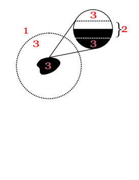
Figure 3: For (a collection of) droplets of characteristic size $\ell$, we split the plane into three regions: the near-infinity region $R_{1}=\{x:\text{dist}(x,\mathcal{D})\gg\ell\},$ the near-$\partial\mathcal{D}$ region $R_{2}=\{x:\text{dist}(x,\partial\mathcal{D})\ll\ell\},$ and the intermediate region $R_{3}$ covering the rest of the plane. To show that integral (128) vanishes, we use large-$x$ asymptotics in $R_{1}$, wavy line approximation in $R_{2}$, and uniform convergence in $R_{3}$.

The region $R_{3}$ is the simplest, since here $\delta z=\mathcal{O}(y^{2})$ tends uniformly to zero, while the remaining factors tend uniformly to a finite limit. Thus the integral over this bounded region vanishes as $\mathcal{O}(\bar{y}^{2})$.

The region $R_{1}$ consists of points $x$ with $|x|$ much larger than the characteristic size of $\mathcal{D}$. In this case a more careful analysis is needed, since we must check that the integral converges near infinity. First we estimate $z$ by

$$z=\frac{1}{2}-\frac{1}{\pi}\frac{y^{2}}{(x^{2}+y^{2})^{2}}\ast\chi_{\mathcal{D}}<\frac{1}{2}-\frac{1}{4\pi}\frac{y^{2}}{x^{4}}\ast\chi_{\mathcal{D}}\,,$$ (129)

where $\chi_{\mathcal{D}}$ is the characteristic function, equal $1$ on $\mathcal{D}$ and $0$ outside. This estimate is true as long as $y$ is smaller than $\text{dist}(x,\mathcal{D})$, and thus applies in $R_{1}$ for $y\lesssim\ell$. From this estimate we get

$$\frac{y^{2}}{\frac{1}{4}-z^{2}}\lesssim\left(\frac{1}{x^{4}}\ast\chi_{\mathcal{D}}\right)^{-1}=\mathcal{O}(x^{4})\,.$$ (130)

Further, we have

$$|V_{i}| \lesssim\frac{|x|}{(x^{2}+y^{2})^{2}}\ast\chi_{\mathcal{D}}\,=\mathcal{O}(|x|^{-3})\,,$$

$$|U_{i}| \lesssim\frac{|x|}{x^{2}+y^{2}}\ast\chi_{\mathcal{D}}\,=\mathcal{O}(|x|^{-1})\,.$$ (131)

Finally, from (131) and (129) we can also conclude that

$$\delta V_{i}=\mathcal{O}(|x|^{-3})\,\,,\quad\delta U_{i}=\mathcal{O}(|x|^{-1})\,,\quad\delta z=\mathcal{O}(y^{2}|x|^{-4})\,.$$ (132)

Combining all these estimates, we see that the integrand in (128) is $\mathcal{O}(y^{2}|x|^{-4})$. Thus the integral over $R_{1}$ is convergent and tends to zero as $\mathcal{O}(\bar{y}^{2}).$

Finally consider the region $R_{2}$, consisting of points $x$ which are much closer to $\partial\mathcal{D}$ than the droplet size. In this region we can neglect the curvature of the boundary. Without loss of generality, we will orient the axes so that the droplet covers the lower half-plane (up to higher-order terms). The situation now becomes identical to the wavy line approximation used in Section 3.6. Borrowing results from that section, we obtain the following estimates for various factors in (128):

$$\frac{y^{2}}{\frac{1}{4}-z^{2}} =\mathcal{O}(r^{2})\,,\qquad V_{i}=\mathcal{O}(r^{-1})\,,$$

$$\delta V_{i} =\mathcal{O}(r^{-2})\,,\qquad\delta U_{i}=\mathcal{O}(1)\,,$$ (133)

$$\delta z =\mathcal{O}(y^{2}r^{-3})\,.$$

For example, the last of these estimates is obtained from (80) as follows:

$$|\delta z(x_{1},x_{2},y)| =\frac{y^{2}}{2r^{3}}\left|\int\frac{dp}{2\pi}e^{-ipx_{1}}(1+r|p|)e^{-r|p|}\varepsilon(p)\right|\,$$

$$\leq\frac{y^{2}}{2r^{3}}\max_{p}\left[\left(1+r|p|\right)e^{-r|p|}\right]\int\frac{dp}{2\pi}|\varepsilon(p)|\,,$$ (134)

which gives us the required estimate under the natural assumption that the perturbation $\varepsilon(x)$ is smooth, so that the Fourier tranform $\varepsilon(p)$ is integrable. The estimates for $\delta V_{i}$ and $\delta U_{i}$ can be proved in exactly the same way. In the case of $\delta U_{i}$ one should use the following Fourier transform expressions (see [2], Appendix B)

$$\delta U_{1}(p) =\frac{x_{2}}{r}e^{-r|p|}\varepsilon(p)\,,$$

$$\delta U_{2}(p) =i(\text{Sign}p)e^{-r|p|}\varepsilon(p)\,.$$ (135)

Using (133), we see that the integrand of (128) is $\mathcal{O}(y^{2}r^{-2}).$ This gives the following upper bound for the integral over $R_{2}$:

$$\oint_{\partial\mathcal{D}}ds\int_{-\infty}^{\infty}dx_{\perp}\frac{y^{2}}{x_{\perp}^{2}+y^{2}}=\mathcal{O}(y),$$ (136)

and we conclude that this part of (128) also vanishes as $\bar{y}\rightarrow 0.$ The proof of (128) is now complete.

A.4 Existence of solutions for $\lambda$ and $\tilde{\lambda}$

In this section we prove that (111) always admits a solution. To show this, we use the following explicit form of $\delta U|_{y=0}$, which follows directly from (35):

$$\delta U_{i}(x) =\frac{1}{\pi}\sum_{b=1}^{B}\oint_{\gamma^{(b)}}K_{i}\left(x-\gamma^{(b)}(s)\right)\delta\gamma_{\perp}^{(b)}(s)\,ds\,,$$

$$K_{i}(x) =\frac{\varepsilon_{ij}x_{j}}{x^{2}}\,.$$ (137)

Here we use the same notation as in (51) to parametrize $\partial\mathcal{D}$ and its pertubations, which are as usual assumed to satisfy the constraints (52).

Now we observe that the convolution kernel in (137) is closed away from the origin:

$$\varepsilon_{ij}\partial_{i}K_{j}=\partial_{i}\frac{x_{i}}{x^{2}}=2\pi\,\delta^{(2)}(x)\,.$$ (138)

From this it follows that the integral of $K$ over a closed contour $\Gamma$ depends only on its winding number $n$ around the origin:

$$\oint_{\Gamma}K=2\pi n\,.\,$$ (139)

Using this in (137), we get

$$\oint_{\Gamma}\delta U=0$$ (140)

for any closed contour lying entirely in $\mathcal{D}$ or $\mathcal{D}^{c}.$ Indeed, such a contour will have definite winding numbers $n^{(b)}$ around every component of $\partial\mathcal{D}$. The integral in (140) will be given by a linear combination of constraints (52) with these winding numbers as coefficients, and thus vanishes.

Eq. (140) applied to arbitrary topologically trivial contours $\Gamma$ implies that $\delta U$ is closed, which guarantees that (111) has a solution locally. Applied to topologically nontrivial contours, (140) shows that this local solution has trivial monodromy and is thus global, which concludes the argument (see Fig. 4).

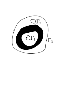
Figure 4: The vector field $\delta U$ has vanishing integrals over topologically trivial ($\Gamma_{1,2}$) as well as nontrivial ($\Gamma_{3}$) contours in the complement of $\partial\mathcal{D}$. This is enough to show that (111) has a global solution.

A.5 Limits on $\partial\mathcal{D}$

It is obvious from (34), (35) that $B,\tilde{B},U$ stay finite when $y\rightarrow 0$, at least when $x\notin\partial D$. Consequently, their perturbations $\delta B,\delta\tilde{B},\delta U$ will also have finite $y=0$ limits. In this section we study how these latter limiting values behave on $\partial\mathcal{D}$. Similarly to how we analyzed region $R_{3}$ in Appendix A.3, we can neglect the curvature of the boundary in the limit $x\rightarrow\partial\mathcal{D}$, and use the wavy line approximation of Section 3.6.

The Fourier transforms of $\delta B_{i}$ and $\delta\tilde{B}_{i}$ with respect to the longitudinal variable $x_{1}$ are given by (84), where we have to put $y=0.$ These Fourier transforms are manifestly continuous at $x_{2}=0.$ Thus we conclude that $\delta B_{i}$ and $\delta\tilde{B}_{i}$ are continuous across $\partial\mathcal{D}.$

The Fourier transforms of $\delta U_{i}$ are given by (135). Setting $y=0,$ we see that $\delta U_{2}$ is continuous at $x_{2}=0$, while $\delta U_{1}$ has a jump discontinuity:

$$\delta U_{1}^{\pm}=\pm\varepsilon\,.$$ (141)

This is in agreement with (116), since $\delta U_{\|}=-\delta U_{1}$ corresponds to the positive orientation of the droplet boundary.

References

-
[1]
J. M. Maldacena, “The large limit of
superconformal field theories and supergravity,” Adv. Theor. Math. Phys. 2, 231 (1998) [arXiv:hep-th/9711200].
S. S. Gubser, I. R. Klebanov and A. M. Polyakov, “Gauge theory correlators from non-critical string theory,” Phys. Lett. B 428, 105 (1998) [arXiv:hep-th/9802109].
E. Witten, “Anti-de Sitter space and holography,” Adv. Theor. Math. Phys. 2, 253 (1998) [arXiv:hep-th/9802150]. - [2] L. Grant, L. Maoz, J. Marsano, K. Papadodimas and V. S. Rychkov, “Minisuperspace quantization of “Bubbling AdS” and free fermion droplets,” JHEP 0508, 025 (2005) [arXiv:hep-th/0505079].
- [3] C. W. Misner, “Minisuperspace,” in Magic Without Magic: John Archibald Wheeler, Ed. J. R. Klauder (Freeman, San Francisco 1972), p. 441.
- [4] H. Lin, O. Lunin and J. Maldacena, “Bubbling AdS space and 1/2 BPS geometries,” JHEP 0410, 025 (2004) [arXiv:hep-th/0409174].
- [5] G. Mandal, “Fermions from half-BPS supergravity,” arXiv:hep-th/0502104.
- [6] B. C. Palmer and D. Marolf, “Counting supertubes,” JHEP 0406, 028 (2004) [arXiv:hep-th/0403025].
- [7] S. Corley, A. Jevicki and S. Ramgoolam, “Exact correlators of giant gravitons from dual SYM theory,” Adv. Theor. Math. Phys. 5, 809 (2002) [arXiv:hep-th/0111222].
- [8] D. Berenstein, “A toy model for the AdS/CFT correspondence,” JHEP 0407, 018 (2004) [arXiv:hep-th/0403110].
- [9] Č. Crnković and E. Witten, “Covariant Description Of Canonical Formalism In Geometrical Theories,” in Three hundred years of gravitation, Eds. S.W. Hawking and W. Israel (Cambridge University Press, 1987), p.676.
- [10] G. J. Zuckerman, “Action Principles And Global Geometry,” in Mathematical Aspects Of String Theory, San Diego 1986, Proceedings, Ed. S.-T. Yau (Worls Scientific, 1987), p.259.
- [11] O. Lunin, J. Maldacena and L. Maoz, “Gravity solutions for the D1-D5 system with angular momentum,” arXiv:hep-th/0212210.
- [12] See S. D. Mathur “The fuzzball proposal for black holes: An elementary review,” arXiv:hep-th/0502050, and references therein.
- [13] M. Taylor, “General 2 charge geometries,” arXiv:hep-th/0507223.
- [14] J. T. Liu, D. Vaman and W. Y. Wen, “Bubbling 1/4 BPS solutions in type IIB and supergravity reductions on ,” arXiv:hep-th/0412043.
-
[15]
D. Martelli and J. F. Morales, “Bubbling
AdS(3),” JHEP 0502, 048 (2005)
[arXiv:hep-th/0412136];
J. T. Liu and D. Vaman, “Bubbling 1/2 BPS solutions of minimal six-dimensional supergravity,” arXiv:hep-th/0412242. - [16] Z. W. Chong, H. Lu and C. N. Pope, “BPS geometries and AdS bubbles,” Phys. Lett. B 614, 96 (2005) [arXiv:hep-th/0412221].
-
[17]
O. Lunin, “Adding momentum to D1-D5 system,” JHEP 0404 (2004) 054 [arXiv:hep-th/0404006];
S. Giusto, S. D. Mathur and A. Saxena, “Dual geometries for a set of 3-charge microstates,” Nucl. Phys. B 701 (2004) 357 [arXiv:hep-th/0405017];
S. Giusto, S. D. Mathur and A. Saxena, “3-charge geometries and their CFT duals,” Nucl. Phys. B 710 (2005) 425 [arXiv:hep-th/0406103];
I. Bena and P. Kraus, “Microstates of the D1-D5-KK system,” Phys. Rev. D 72 (2005) 025007 [arXiv:hep-th/0503053];
I. Bena and N. P. Warner, “Bubbling supertubes and foaming black holes,” arXiv:hep-th/0505166;
P. Berglund, E. G. Gimon and T. S. Levi, “Supergravity microstates for BPS black holes and black rings,” arXiv:hep-th/0505167;
I. Bena and N. P. Warner, “One ring to rule them all … and in the darkness bind them?,” arXiv:hep-th/0408106;
S. Giusto and S. D. Mathur, “Geometry of D1-D5-P bound states,” arXiv:hep-th/0409067. -
[18]
I. Bena and P. Kraus, “Three charge supertubes and black
hole hair,” Phys. Rev. D 70, 046003 (2004)
[arXiv:hep-th/0402144];
D. Bak, Y. Hyakutake, S. Kim and N. Ohta, “A geometric look on the microstates of supertubes,” Nucl. Phys. B 712, 115 (2005) [arXiv:hep-th/0407253];
H. Elvang, R. Emparan, D. Mateos and H. S. Reall, “Supersymmetric black rings and three-charge supertubes,” Phys. Rev. D 71 (2005) 024033 [arXiv:hep-th/0408120]. - [19] I. Bena and P. Kraus, “Microscopic description of black rings in AdS/CFT,” JHEP 0412 (2004) 070 [arXiv:hep-th/0408186].
- [20] R. Arnowitt, S. Deser and C. W. Misner, “The Dynamics Of General Relativity,” in Gravitation: an introduction to current research, Ed. L. Witten (Wiley 1962), p.227 [arXiv:gr-qc/0405109].
- [21] J. Lee and R. M. Wald, “Local Symmetries And Constraints,” J. Math. Phys. 31, 725 (1990).
- [22] G. W. Gibbons and S. W. Hawking, “Action Integrals And Partition Functions In Quantum Gravity,” Phys. Rev. D 15, 2752 (1977).
- [23] L. D. Landau and E. M. Lifshitz, The Classical Theory of Fields, (Butterworth-Heinemann, 1980)
- [24] V.I. Arnold, Mathematical Methods of Classical Mechanics, Springer, 1997.
- [25] K. Kuchař, “Canonical Quantization Of Cylindrical Gravitational Waves,” Phys. Rev. D 4, 955 (1971).
- [26] G. A. Mena Marugán and M. Montejo, “Quantization of pure gravitational plane waves,” Phys. Rev. D 58, 104017 (1998) [arXiv:gr-qc/9806105].
- [27] N. S. Manton, “A Remark On The Scattering Of BPS Monopoles,” Phys. Lett. B 110, 54 (1982).
- [28] M. F. Atiyah and N. J. Hitchin, “Low-Energy Scattering Of Nonabelian Monopoles,” Phys. Lett. A 107, 21 (1985).
- [29] G. W. Gibbons and P. J. Ruback, “The Motion Of Extreme Reissner-Nordstrom Black Holes In The Low Velocity Limit,” Phys. Rev. Lett. 57, 1492 (1986).
- [30] R. C. Ferrell and D. M. Eardley, “Slow Motion Scattering And Coalescence Of Maximally Charged Black Holes,” Phys. Rev. Lett. 59, 1617 (1987).
- [31] S. M. Lee, S. Minwalla, M. Rangamani and N. Seiberg, “Three-point functions of chiral operators in , SYM at large ,” Adv. Theor. Math. Phys. 2, 697 (1998) [arXiv:hep-th/9806074].
- [32] H. J. Kim, L. J. Romans and P. van Nieuwenhuizen, “The Mass Spectrum Of Chiral Supergravity On ,” Phys. Rev. D 32, 389 (1985).
- [33] R. R. Metsaev and A. A. Tseytlin, “Exactly solvable model of superstring in plane wave Ramond-Ramond background,” Phys. Rev. D 65, 126004 (2002) [arXiv:hep-th/0202109].
-
[34]
K. V. Kuchař and M. P. Ryan, “Can Mini Superspace
Quantization Be Justified?,” in Gravitational Collapse And Relativity, Kyoto 1986, Proceedings, Eds. H. Sato and T. Nakamura (World Scientific,
Singapore, 1986), p.451.
K. V. Kuchař and M. P. Ryan, “Is Minisuperspace Quantization Valid?: Taub In Mixmaster,” Phys. Rev. D 40, 3982 (1989). - [35] X.-G. Wen, “Topological orders and Edge excitations in FQH states”, arXiv:cond-mat/9506066.
-
[36]
S. Iso, D. Karabali and B. Sakita,
“Fermions in the lowest Landau level: Bosonization, algebra,
droplets, chiral bosons,”
Phys. Lett. B 296, 143 (1992)
[arXiv:hep-th/9209003];
A. P. Polychronakos, “Chiral actions from phase space (quantum Hall) droplets,” Nucl. Phys. B 705, 457 (2005) [arXiv:hep-th/0408194]. - [37] A. Dhar, “Bosonization of non-relativistic fermions in 2-dimensions and collective field theory,” arXiv:hep-th/0505084.
- [38] L. Maoz, V. S. Rychkov and A. Shomer, in progress.
- [39] B. de Wit, H. Samtleben and M. Trigiante, “Magnetic charges in local field theory,” arXiv:hep-th/0507289.