RIKEN-TH-46

August 2005

The work is dedicated to A.Polyakov. I believe that

Sasha will recognize many of his “low-dimensional”

ideas behind the present development.

Abstract

General properties of perturbed conformal field theory interacting with quantized Liouville gravity are considered in the simplest case of spherical topology. We discuss both short distance and large distance asymptotic of the partition function. The crossover region is studied numerically for a simple example of the perturbed Yang-Lee model, complemented in general with arbitrary conformal “spectator” matter. The latter is not perturbed and remains conformal along the flow, thus giving a control over the Liouville central charge. The partition function is evaluated numerically from combined analytic and perturbative information. In this paper we use the perturbative information up to third order. At special points the four-point integral can be evaluated and compared with our data. At the solvable point of minimal Liouville gravity we are in remarkably good agreement with the matrix model predictions. Possibilities to compare the result with random lattice simulations is discussed.

1 Introduction

Liouville field theory (LFT) first appeared in the 2D quantum gravity context in the famous paper by Polyakov [1]. It has been demonstrated there that the LFT action appears naturally as the induced action of a conformal field theory living on a two-dimensional surface with non-trivilal background metric. Quantum LFT was recognized as a conformal field theory (CFT) and it is hardly an exaggeration to say that this peculiar example always stayed behind the motivations in the subsequent explosive development of the CFT, triggered by [2]. In particular, this induced LFT action governs a specific dynamics of the 2D quantum gravity, which is now called the critical (or Liouville) gravity. Characteristics of the critical gravity (critical exponents, correlation functions etc.) depend on the central charge of LFT, the last being simply related to the central charge of the inducing conformal matter. As a conformal theory LFT is rather complicated and differs in many important respects from the so called rational CFT’s, developed and studied soon after the pioneering paper [2]. Despite essential progress in understanding of the space of states and hidden symmetries in LFT ([3, 5] or [4]), physical interpretation of the results in terms of fluctuating geometry of 2D surfaces remained unclear.

Meanwhile, a very different approach to 2D quantum gravity has been under development. This approach can be called in general the discrete gravity. A smooth Riemannian manifold is substituted by a “random triangulation”, or more precisely, by a graph of the same topology (and possibly certain “matter” degrees of freedom attached to its vertices or faces) while the Riemann metric is simulated by the geodesic distances along the graph, the total number of vertices (or plaquettes) being interpreted as the surface area. The gravity problem is then reduced to a summation (in the spirit of the path integral) over the ensemble of such graphs. Progress in the study of these discrete models was drastically boosted after invention of a very powerful method to sum up the statistical ensembles of discrete gravity by reducing them to certain integrals over $N\times N$ matrices in the limit $N\rightarrow\infty$ [6, 7, 8]. The latter integrals can be sometimes evalutated explicitly, giving rise to exactly solvable models of discrete gravity. Despite the fact that not every discrete model can be treated by the matrix model approach, progress was so dramatic that now these discrete models are often called the matrix models of 2D gravity. In the limit $N\rightarrow\infty$ many types of critical behavior with different critical exponents had been discovered. Moreover, it is often possible to calculate explicitly the scaling functions which describe the “flows” between different critical points. Another impressive advantage of the discrete approach is that it allows to treat “surfaces” of arbitrary topology. This led even to the study of the grand statistical ensemble of surfaces with different topology, the object of extreme importance in the string theory.

Approximately at the same time the Polyakov’s gravity has been reconsidered in slightly different framework [9] (called sometimes the “Polyakov’s” or “light-cone” gauge), which allowed to derive the critical exponents of this induced gravity in an explicit form (the KPZ scaling). It was soon recognized [10, 11] that the same exponents are exactly reproduced in the original formulation of LFT provided certain finite renormalization of the coupling constant are conjectured and taken into account.

The nexus of the Liouville and discrete approaches to quantum gravity in fact flashed already in ref.[9] in the observation that some critical KPZ exponents are precisely those appearing in the critical behavior of random lattice systems.

Since the very advance of the discrete 2D gravity [6, 7] in 1985, it always challenged the field theoretical community. The ambition is not only to match with its achievements, i.e. learn to evaluate the correlation numbers and the scaling functions (and also to work at higher topologies). To reveal the field theory potential in 2D gravity to its full extent means to go beyond the limits accessible by the matrix models. In this paper I recall the most important steps and problems along this line. A scaling function for the spherical partition function of a perturbed CFT coupled to Liouville gravity is considered as a perturbative sum over the correlation numbers. Although it is still a problem to evaluate directly the whole set of these numbers, general arguments allow to establish important analytic properties of the scaling function. In order, these analytic properties restrict the scaling function to a large extent. In particular, sometimes even a few first orders of the perturbative series allow to reproduce the whole function, approximately but to a remarkably good accuracy.

To my opinion the main lesson to draw from this simple exercise is that the Liouville gravity as formulated on the basis of early Polyakov’s ideas is indeed a consistent and pithy structure whose physical content is rich and definitely extends beyond the relatively dull world offered by the matrix models in their present formulation [12] (recent refreshments can be found in refs.[13]).

2 Perturbed Liouville gravity

Liouville gravity (LG) is the 2D gravity induced by a “critical matter”. Its matter content is described by a certain “matter” CFT $\mathcal{M}_{\text{M}}$ with the central charge $c_{\text{M}}$. In the field theory approach LG is described as a joint CFT $\mathcal{M}_{\text{M}}+$ Liouville $+$ ghosts [1]

$$\mathcal{L}_{\text{LG}}=\mathcal{L}_{\text{M}}+\mathcal{L}_{\text{L}}+\mathcal{L}_{\text{gh}}$$ (2.1)

Conformal Liouville field theory is defined through the local Lagrangian

$$\mathcal{L}_{\text{L}}=\frac{1}{4\pi}(\partial_{a}\phi)^{2}+\mu e^{2b\phi}$$ (2.2)

Its central charge $c_{\text{L}}$ is related to the parameter $b$ as

$$c_{\text{L}}=1+6Q^{2}$$ (2.3)

The combination

$$Q=b^{-1}+b$$ (2.4)

is called the background charge (basically for historical reasons). The scale parameter $\mu$ is called the cosmological constant because in LFT $\exp(2b\phi)d^{2}x$ is interpreted as the quantized area element of the 2D space. The ghost CFT is the usual $BC$ system

$$\mathcal{L}_{\text{gh}}=\frac{1}{\pi}(C\bar{\partial}B+\bar{C}\partial\bar{B})$$ (2.5)

of spin $(2,-1)$ and central charge $c_{\text{gh}}=-26$ [1]. The gravity interpretation requires the total central charge of the joint CFT (2.1) to be $0$. In other words, parameter $b$ in (2.2) is determined from the “central charge balance” equation

$$c_{\text{L}}+c_{\text{M}}=26$$ (2.6)

Presently we are going to consider the perturbed Liouville gravity where the matter is not critical but described as a perturbed CFT

$$\mathcal{L}_{\text{matter}}=\mathcal{L}_{\text{M}}+\frac{\lambda}{2\pi}\Phi$$ (2.7)

Here $\Phi$ is some relevant primary field from the spectrum of the matter CFT of dimension $\Delta$ and $\lambda$ is the corresponding coupling constant. It seems natural to take a simple solvable model of CFT as the unperturbed matter field theory, e.g., one of the famous minimal models $M_{p/p^{\prime}}$ [2]. The perturbing field is then one of the relevant degenerate fields of this minimal model and its correlation functions are either known explicitly or constructible in principle. The matter central charge takes the worldwide known value $c=c_{p,p^{\prime}}$ and therefore the Liouville parameters are rigidly fixed by (2.6). E.g., if the matter CFT is the free Majorana fermion CFT $\mathcal{M}_{1/2}$ the Liouville parameter is a number $b=\sqrt{3/4}$ and no more a parameter. For example, a question like “what is the physics of free fermion coupled to almost classic gravity?” cannot be addressed. From theoretical point of view it seems convenient to lift this restriction and get an independent control over the Liouville parameters. To this order let us add to the matter content of the theory another conformal matter of central charge $c_{\text{sp}}$. This matter is unperturbed and always remain conformal. Therefore it formally does not interact neither with the Liouville mode (except for through the conformal anomaly) nor with the perturbed CFT (2.7). Its main role is to contribute to the central charge balance (2.6). For this reason we call it the “spectator” matter. To be precise, there is also some connection via conformal moduli. However in the simplest case of the spherical geometry (which we mainly address presently) any details of this “spectator” CFT except for its central charge are of no importance. It can equally well be considered as a formal shapeless ingredient seen only through $c_{\text{sp}}$. In the last section we’ll discuss possible realizations of the spectator matter.

With this additional liberty the total matter central charge is

$$c_{\text{M}}=c+c_{\text{sp}}$$ (2.8)

and the perturbed Liouville gravity is expressed symbolically through the Lagrangian

$$\mathcal{L}_{\lambda}=\mathcal{L}_{\text{CFT}}+\mathcal{L}_{\text{L}}+\frac{\lambda}{2\pi}\Phi e^{2g\phi}+\mathcal{L}_{\text{sp}}+\mathcal{L}_{\text{gh}}$$ (2.9)

As explained above, in the spherical case the last two terms in (2.9) are coupled only through the conformal anomaly. Therefore we will omit these background degrees of freedom, having in mind that they enter the central charge balance, which is solved for $b$ as

$$b=\sqrt{\frac{25-c_{\text{M}}}{24}}-\sqrt{\frac{1-c_{\text{M}}}{24}}$$ (2.10)

For the branch chosen the semiclassical regime $b\rightarrow 0$ is achieved when $c_{\text{sp}}\rightarrow-\infty$. In this limit the background space is in fact a classical symmetric sphere. Otherwise this parameter $b$ characterizes the “rigidity” of the space with respect to quantum fluctuations.

Interaction with the Liouville gravity “dresses” the perturbing primary field $\Phi$ with an appropriate Liouville exponential field $\exp(2g\phi)$. Parameter $g$ is determined from the following kinematic requirement

$$g(Q-g)+\Delta=1$$ (2.11)

which means simply that the composite field

$$U=\Phi e^{2g\phi}$$ (2.12)

is a $(1,1)$ form and can be integrated over the space. Ordinarily the least of the two roots is chosen

$$g=\sqrt{\frac{25-c_{\text{M}}}{24}}-\sqrt{\frac{1-c_{\text{M}}}{24}+\Delta}$$ (2.13)

Notice that $g$ is positive for relevant perturbations $\Delta<1$ (and negative for the irrelevant ones).

3 Spherical partition function

The spherical partition function $Z(\mu,0)$ of the Liouville gravity is known to scale as

$$Z(\mu,0)=\mu^{Q/b}Z(1,0)$$ (3.1)

with some dimensionless constant $Z(1,0)$. It is easy to see that the perturbing coupling constant $\lambda$ scales as $\mu^{1/\rho}$ with positive

$$\rho=bg^{-1}$$ (3.2)

The perturbed partition function $Z(\mu,\lambda)$ introduces the scaling function $\mathcal{Z}$ of the dimensionless combination $\lambda\mu^{-1/\rho}$

$$Z(\mu,\lambda)=\mu^{Q/b}\mathcal{Z}\left(\lambda\mu^{-1/\rho}\right)$$ (3.3)

This scaling function is the main object of our present study. Sometimes it will be more convenient to consider the “fixed area” partition function $Z_{A}(\lambda)$ defined as the inverse Laplace transform of $Z(\mu,\lambda)$

$$Z_{A}(\lambda)=A\int_{\uparrow}\frac{d\mu}{2\pi i}Z(\mu,\lambda)e^{\mu A}$$ (3.4)

where the contour $\uparrow$ goes along the imaginary axis to the right from all singularities of the integrand. In particular, in the critical gravity

$$Z_{A}(0)=Z(1,0)\int_{\uparrow}\frac{d\mu}{2\pi i}\mu^{Q/b}e^{\mu A}=\frac{Z(1,0)}{\Gamma(-Qb^{-1})}A^{-Q/b}$$ (3.5)

Inversely

$$Z(\mu,\lambda)=\int_{(0)}^{\infty}Z_{A}(\lambda)e^{-\mu A}\frac{dA}{A}$$ (3.6)

where $(0)$ at the lower limit indicates that the integral is often divergent at small $A$ and (3.6) means a properly regularized version. The name “fixed area” is motivated by the interpretation of the integral

$$A=\int e^{2b\phi}d^{2}x$$

as the total area of the gravitating sphere. For the same reasons as for $Z(\mu,\lambda)$ the fixed area partition function has similar scaling form

$$Z_{A}(\lambda)=Z_{A}(0)z(h)$$ (3.7)

where it happens more convenient to normalize the scale invariant parameter $h$ as

$$h=\lambda\left(\frac{A}{\pi}\right)^{1/\rho}$$ (3.8)

4 UV expansion

Partition function (3.3) is a regular series in the coupling constant $\lambda$

$$\mathcal{Z}(\mu,\lambda)=\sum_{n=0}^{\infty}a_{n}\left(-\lambda\right)^{n}$$ (4.1)

Each term in this expansion is determined by the corresponding order in the interaction (2.12). The coefficients

$$a_{n}=\frac{Z^{-1}(\mu,0)}{(2\pi)^{n}n!}\int_{M_{n}}\left\langle U^{n}\right\rangle$$ (4.2)

are the integrated (and normalized) correlation functions of $n$ insertions of the composite (2.12). According to (3.3) the coefficients $a_{n}$ scale as $a_{n}\sim\mu^{-n/\rho}$. In the LFT approach the source correlation functions (i.e., the coordinate dependent functions before the integration) factorize into a product

$$\left\langle U(x_{1})\ldots U(x_{n})\right\rangle=\left\langle\Phi(x_{1})\ldots\Phi(x_{n})\right\rangle_{\text{M}}\left\langle e^{2g\phi(x_{1})}\ldots e^{2g\phi(x_{n})}\right\rangle_{\text{L}}$$ (4.3)

as it can be literally read off from the action (2.9). The integral in (4.2) is not over the positions of all $n$ insertions but rather over the $n-3$ dimensional moduli space $M_{n}$ of the sphere with $n$ punctures. Practically at $n\geq 3$ this amounts to place any $3$ insertions of $U$ at arbitrary fixed points $x_{1}$, $x_{2}$ and $x_{3}$ and integrate over the positions of the remaining $n-3$ ones

$$\int_{M_{n}}\left\langle U^{n}\right\rangle=\int\left\langle W(x_{1})W(x_{2})W(x_{3})U(x_{4})\ldots U(x_{n)}\right\rangle d^{2}x_{4}\ldots d^{2}x_{n}$$ (4.4)

Following the standard string theory practice we have also replaced the “nailed” insertions $U(x_{1})$ by $W(x_{i})=C\bar{C}U(x_{i})$ to get rid of the redundant dependence on their positions and also to give the integrand the total ghost number $3$ (as it is required by the ghost number conservation). Simplest example is the three-point function, where the moduli space is empty and the three-point function is simply the product

$$\left\langle U^{3}\right\rangle=\left\langle C\bar{C}(x_{1})C\bar{C}(x_{2})C\bar{C}(x_{3})\right\rangle_{\text{gh}}\left\langle\Phi(x_{1})\Phi(x_{2})\Phi(x_{3})\right\rangle_{\text{M}}\left\langle e^{2g\phi(x_{1})}e^{2g\phi(x_{2})}e^{2g\phi(x_{3})}\right\rangle_{\text{L}}$$ (4.5)

Two- and zero-point functions are simply figured out from the three-point one (see below).

In the exactly solvable CFT models all multipoint correlation functions are in principle constructible. They are determined uniquely once the normalization of the primary fields is fixed. In what follows we use the standard CFT normalization of the matter fields through the two-point function

$$\left\langle\Phi(x_{1})\Phi(x_{2})\right\rangle_{\text{M}}=\left|x_{1}-x_{2}\right|^{-4\Delta}$$ (4.6)

The field normalization also gives precise meaning to the coupling constant $\lambda$ in (2.7) and (2.9).

In practice, even in solvable CFT’s, it is usually difficult to go explicitly beyond the four-point functions (except for such special cases as the free-field CFT’s). At the same time the one-, two- and three-point functions are rather universal. Conventional CFT wisdom requires the one point function to vanish

$$\left\langle\Phi(x)\right\rangle_{\text{M}}=0$$ (4.7)

while the three-point function is fixed up to an overall constant $C_{\Phi\Phi\Phi}$

$$\left\langle\Phi(x_{1})\Phi(x_{2})\Phi(x_{3})\right\rangle_{\text{M}}=\frac{C_{\Phi\Phi\Phi}}{\left|x_{12}x_{23}x_{32}\right|^{2\Delta}}$$ (4.8)

which is called the three-$\Phi$ structure constant and is usually known explicitly in solvable CFT’s. In (4.8) and often below we use the abbreviated notation $x_{kl}=x_{k}-x_{l}$. Higher correlation functions have less universal form. The four-point case is more handy and allows explicit channel decompositions, e.g.,

$$\left\langle\Phi(x_{1})\Phi(x_{2})\Phi(x_{3})\Phi(x_{4})\right\rangle_{\text{M}}=\frac{G_{\text{M}}(x,\bar{x})}{\ \left|x_{14}x_{23}\right|^{4\Delta}}$$ (4.9)

$$G_{\text{M}}(x,\bar{x}) =\sum_{i}C_{\Phi\Phi}^{i}C_{\Phi\Phi i}\mathcal{F}\left(\begin{array}[c]{cc}\Delta&\Delta\\ \Delta&\Delta\end{array}\left|\Delta_{i}\right|x\right)\mathcal{F}\left(\begin{array}[c]{cc}\Delta&\Delta\\ \Delta&\Delta\end{array}\left|\Delta_{i}\right|\bar{x}\right)$$ (4.14)

in terms of the structure constants and the four-point conformal blocks related to the conformal algebra with central charge $c$ [2]

$$\mathcal{F}\left(\begin{array}[c]{cc}\Delta&\Delta\\ \Delta&\Delta\end{array}\left|\Delta_{i}\right|x\right)=\raisebox{-33.12117pt}{\includegraphics[height=73.75099pt,width=154.31038pt]{mblock.eps}}$$ (4.15)

These blocks are holomorphic in the projective invariant

$$x=\frac{(x_{1}-x_{2})(x_{3}-x_{4})}{(x_{1}-x_{4})(x_{3}-x_{2})}$$ (4.16)

The sum in (4.9) is over all primary fields $\left\{\Phi_{i},\Delta_{i}\right\}$ entering the operator product expansion of $\Phi(x)\Phi(0)$.

The situation is nearly the same in LFT. The three-point functions are known explicitly [14] for arbitrary exponential operators $\exp(2a\phi)$ (the basic primary fields of LFT)

$$\left\langle e^{2a_{1}\phi(x_{1})}e^{2a_{2}\phi(x_{2})}e^{2a_{3}\phi(x_{3})}\right\rangle_{\text{L}}=\frac{C_{\text{L}}(a_{1},a_{2},a_{3})}{\left|x_{12}\right|^{2\Delta_{1}+2\Delta_{2}-2\Delta_{3}}\left|x_{23}\right|^{2\Delta_{3}+2\Delta_{4}-2\Delta_{1}}\left|x_{31}\right|^{2\Delta_{3}+2\Delta_{1}-2\Delta_{2}}}$$ (4.17)

where

$$\Delta_{i}=a_{i}(Q-a_{i})$$ (4.18)

are the dimensions of the LFT exponential fields and the constant (letter $a$ below stands for $a_{1}+a_{2}+a_{3}$)

$$\ C_{\text{L}}(a_{1},a_{2},a_{3})=\left(\pi\mu\gamma(b^{2})b^{2-2b^{2}}\right)^{(Q-a)/b}\frac{\Upsilon_{b}(b)}{\Upsilon_{b}(a-Q)}\prod_{i=1}^{3}\frac{\Upsilon_{b}(2a_{i})}{\Upsilon_{b}(a-2a_{i})}$$ (4.19)

is expressed in terms of certain special function $\Upsilon_{b}(x)$, which is an entire function related to the Barnes double gamma function. It’s defining properties are the shift relations

$$\Upsilon_{b}(x+b) =\gamma(bx)b^{1-2bx}\Upsilon_{b}(x)$$ (4.20)

$$\Upsilon_{b}(x+b^{-1}) =\gamma(b^{-1}x)b^{-1+2b^{-1}x}\Upsilon_{b}(x)$$

It is also symmetric w.r.t. the reflection $x\rightarrow Q-x$ and self-dual (i.e., invariant w.r.t. $b\rightarrow b^{-1}$) as a function of the parameter $b$. Integral representation, which fixes also the overall normalization can be found e.g. in [15]. In (4.19) and throughout the paper $\gamma(x)$ is the usual little $\gamma$-function. The LFT four-point function

$$\left\langle e^{2a_{1}\phi(x_{1})}e^{2a_{2}\phi(x_{2})}e^{2a_{3}\phi(x_{3})}e^{2a_{4}\phi(x_{4})}\right\rangle_{\text{LFT}}=$$ (4.21)

$$\ \ \frac{\left|x_{24}\right|^{2(\Delta_{1}+\Delta_{3}-\Delta_{2}-\Delta_{4})}\left|x_{34}\right|^{2(\Delta_{1}+\Delta_{2}-\Delta_{3}-\Delta_{4})}}{\left|x_{14}\right|^{4\Delta_{1}}\left|x_{23}\right|^{2(\Delta_{1}+\Delta_{2}+\Delta_{3}-\Delta_{4})}}\ G_{\text{L}}\left(\left.\begin{array}[c]{cc}a_{1}&a_{3}\\ a_{2}&a_{4}\end{array}\right|x,\bar{x}\right)$$ (4.24)

also allows holomorphic antiholomorphic decomposition [15], similar to (4.9)

$$G_{\text{L}}\left(\left.\begin{array}[c]{cc}a_{1}&a_{3}\\ a_{2}&a_{4}\end{array}\right|x,\bar{x}\right)=$$ (4.27)

$$\ \ \ \ \ \int\frac{dP}{4\pi}C_{\text{L}}\left(a_{1},a_{2},\frac{Q}{2}+iP\right)C_{\text{L}}\left(\frac{Q}{2}-iP,a_{3},a_{4}\right)\mathcal{F}_{P}\left(\left.\begin{array}[c]{cc}\Delta_{1}&\Delta_{3}\\ \Delta_{2}&\Delta_{4}\end{array}\right|x\right)\mathcal{F}_{P}\left(\left.\begin{array}[c]{cc}\Delta_{1}&\Delta_{3}\\ \Delta_{2}&\Delta_{4}\end{array}\right|\bar{x}\right)$$ (4.32)

In (4.21) and (4.27) $\Delta_{i}$ with $i=1,\ldots,4$ are the LFT dimensions (4.18).The integral now is over a continuous spectrum of irreducible representations of the Virasoro algebra with central charge $c_{\text{L}}$ and dimension $Q^{2}/4+P^{2}$. The corresponding four-point blocks

$$\mathcal{F}_{P}\left(\left.\begin{array}[c]{cc}\Delta_{1}&\Delta_{3}\\ \Delta_{2}&\Delta_{4}\end{array}\right|x\right)=\raisebox{-34.12578pt}{\includegraphics[height=75.12502pt,width=164.18994pt]{lblock.eps}}$$ (4.33)

are related to the conformal algebra with the Liouville central charge $c_{\text{L}}$.

Application of eq.(4.4) is not straightforward at $n<3$. The moduli space has formally negative dimension and this is related to the non-trivial space of conformal Killing vector fields on the sphere with $2$ and $0$ punctures. The simplest way to determine the correlation functions with $n<3$ is to differentiate them sufficiently many times with respect to $\mu$ (each differentiation introduces an insertion of the area-element field $\exp(2b\phi)$) until the order of the correlation function attains $n\geq 3$.This maneuver is quite a common way to treat the zero-mode problem of the sphere. In the case of the two-point function it’s enough to differentiate once

$$-\frac{\partial}{\partial\mu}\left\langle e^{2g\phi}e^{2g\phi}\right\rangle_{\text{L}}=C_{\text{L}}(g,g,b)=\left(\pi\mu\gamma(b^{2})\right)^{(Q-2g)/b}\frac{\gamma(2gb-b^{2})\gamma(2gb^{-1}-b^{-2})}{\pi\mu b}$$ (4.34)

After an integration in $\mu$

$$\left\langle e^{2g\phi}e^{2g\phi}\right\rangle_{\text{L}}=-\left(\pi\mu\gamma(b^{2})\right)^{(Q-2g)/b}\frac{\gamma(2gb-b^{2})\gamma(2gb^{-1}-b^{-2})}{\pi(Q-2g)}$$ (4.35)

This expression does not coincide with the Liouville reflection amplitude LABEL:AAl

$$R(g)=-\left(\pi\mu\gamma(b^{2})\right)^{(Q-2g)/b}\frac{\gamma(2gb-b^{2})\gamma\left(2gb^{-1}-b^{-2}\right)}{\left(2g-Q\right)^{2}}$$ (4.36)

(which is ordinarily associated with the two-point function in LFT) differing in the factor of $\pi^{-1}(Q-2g)$. Similar wisdom gives for the Liouville partition function

$$-\frac{\partial^{3}}{\partial\mu^{3}}Z_{\text{L}}=C_{\text{L}}(b,b,b)=-\left(\pi\mu\gamma(b^{2})\right)^{Q/b}\frac{\left(b^{-2}-1\right)^{2}}{\pi^{3}\mu^{3}b\gamma(b^{2})\gamma\left(b^{-2}\right)}$$ (4.37)

and hence

$$Z_{\text{L}}=\left(\pi\mu\gamma(b^{2})\right)^{Q/b}\frac{(1-b^{2})}{\pi^{3}Q\gamma(b^{2})\gamma(b^{-2})}$$ (4.38)

Notice that this expression in not self-dual, unlike the three-point function itself. This fact looks somewhat surprising in the Liouville context and likely needs better understanding. Below we will meet many opportunities to support the consistency of (4.35) and (4.38) in the 2D gravity context. Therefore we have to take this breakdown of the Liouville self-duality in the 2D gravity application as the matter of fact.

After all these preliminaries, we are in the position to construct explicitly few first terms in the perturbative expansion (4.1)

$$a_{0} =1$$

$$a_{1} =0$$ (4.39)

$$a_{2} =\left(\pi\mu\gamma(b^{2})\right)^{-2g/b}\frac{Q\gamma(2gb-b^{2})\gamma(2gb^{-1}-b^{-2})\gamma(b^{2})\gamma(b^{-2})}{8(2g-Q)(1-b^{2})}$$

$$a_{3} =\frac{C_{\Phi\Phi\Phi}C_{\text{L}}(g,g,g)}{48\pi^{3}Z_{\text{L}}}$$

$$a_{4} =\frac{1}{24(2\pi)^{4}Z_{\text{L}}}\int G_{\text{M}}(x,\bar{x})G_{\text{L}}\left(\left.\begin{array}[c]{cc}g&g\\ g&g\end{array}\right|x,\bar{x}\right)d^{2}x$$ (4.42)

$$\ldots$$

In what follows we will be more interested in the fixed area partition function (3.7). The scaling function $z(h)$ has the following perturbative expansion

$$z(h)=\sum_{n=0}^{\infty}z_{n}(-h)^{n}$$ (4.43)

where the dimensionless coefficients $z_{n}$ are related to $a_{n}$ as

$$z_{n}=\frac{(\pi\mu)^{n/\rho}a_{n}\Gamma(-1-b^{-2})}{\Gamma(n\rho^{-1}-b^{-2}-1)}$$ (4.44)

Explicitly up to the third order

$$z_{0} =1$$

$$z_{1} =0$$ (4.45)

$$z_{2} =\left(\gamma(b^{2})\right)^{-2g/b}\frac{\gamma(2gb-b^{2})\gamma(b^{2})\Gamma(b^{-2})}{8(b^{-2}-1)\Gamma(1+b^{-2}-2gb^{-1})}$$

$$z_{3} =\frac{C_{\Phi\Phi\Phi}}{6(2\pi)^{3}}\frac{C_{\text{L}}^{(A=\pi)}(g,g,g)}{Z_{\text{L}}^{(A=\pi)}}$$

In the last expression

$$C_{\text{L}}^{(A)}(g,g,g)=\frac{\left(\pi\gamma(b^{2})b^{2-2b^{2}}A^{-1}\right)^{(Q-3g)/b}\Upsilon(b)\Upsilon^{3}(2g)}{\Upsilon(3g-Q)\Upsilon^{3}(g)\Gamma(3gb^{-1}-1-b^{-2})}$$ (4.46)

is the fixed area $A$ Liouville three-point function and the fixed area partition sum $Z_{\text{LFT}}^{(A)}$ reads

$$Z_{\text{L}}^{(A)}=\left(\frac{\pi\gamma(b^{2})}{A}\right)^{Q/b}\frac{\Gamma(2-b^{2})}{\pi^{3}b^{3}\Gamma(b^{2})\Gamma(b^{-2})}$$ (4.47)

For relevant perturbations (3.8) is small for small area $A$. This means that the perturbative expansion (4.43) in fact determines the behavior of the partition function at small surface area $A$. Notice also that the coefficients $z_{n}$ in (4.44) are suppressed at large $n$ by additional $\Gamma$-function in the denominator as compared with $a_{n}$. This means that if the perturbative series (4.1) is convergent, the fixed area $z(h)$ is an entire function of $h$.

5 Criticality

From physical considerations we expect that at $A\rightarrow\infty$ the fixed area partition function behaves as

$$Z_{A}(\lambda)=Z_{\infty}A^{-Q^{\prime}/b^{\prime}}e^{\mu_{\text{c}}A}$$ (5.1)

where $\mathcal{E}_{\text{vac}}(b)=-\mu_{\text{c}}$ is the specific free energy generated by the massive (finite correlation length) modes of the perturbed CFT $\mathcal{M}_{c}$. For dimensional reasons

$$\mu_{\text{c}}=f_{0}(b)\lambda^{\rho}$$ (5.2)

with some dimensionless $f_{0}(b)$. This perturbed CFT interacts also with the quantized gravity and therefore $\mathcal{E}_{\text{vac}}(b)$ reduces to the vacuum energy $\mathcal{E}_{\text{vac}}(0)$ of the model (2.7) in “rigid” flat background only in the classical limit $b^{2}=0$. Otherwise it depends on $b^{2}$ and appears to be an important characteristic of the matter interacting with quantum gravity. Clearly the grand partition function $Z(\mu,\lambda)$ develops a singularity at $\mu=\mu_{\text{c}}$. Therefore $\mathcal{E}_{\text{vac}}(b)$ is simply another interpretation of the critical point in the cosmological constant (usually referred to as the value of $\mu$ where the surface “blows up”, one of the images convenient to make an illusion of understanding). The related singularity of $Z(\mu,\lambda)$ in the coupling constant $\lambda$ at

$$\lambda_{\text{c}}=\left(\frac{\mu}{f_{0}(b)}\right)^{1/\rho}$$ (5.3)

often happens to be the one closest to the origin. In this case it determines the finite convergence region of the perturbative series (4.1). As it was already mentioned above, this in order implies that the function $z(h)$ is entire.

Let us also assume that the perturbed matter is “massive”, i.e., the correlations of this coupled matter degrees of freedom do not extend far beyond the characteristic mass scale $m_{\text{c}}\sim$ $\lambda^{\rho}$. Then at $A\gg m_{\text{c}}^{-2}$ the “massive” part of the matter “dies out”, i.e., it does not contribute any more to the matter central charge. The gravity dynamics is determined then by the central charge of the “spectator matter”, which doesn’t interact and therefore always remains conformal. Then the infrared parameters $b^{\prime}$ and

$$Q^{\prime}=1/b^{\prime}+b^{\prime}$$ (5.4)

are determined from the equation

$$1+6(Q^{\prime})^{2}+c_{\text{sp}}=26$$ (5.5)

These are the parameters entering the power-like part of the asymptotic (5.1). More explicitly

$$Q^{\prime} =\sqrt{Q^{2}+\frac{c}{6}}$$ (5.6)

$$b^{\prime} =\sqrt{\frac{Q^{2}}{4}+\frac{c}{24}}-\sqrt{\frac{Q^{2}}{4}+\frac{c}{24}-1}$$

In terms of $h$ the asymptotic of the function reads

$$\log z(h)\sim\pi f_{0}(b)h^{\rho}+\rho\left(\frac{Q}{b}-\frac{Q^{\prime}}{b^{\prime}}\right)\log h+\log z_{\infty}+\ldots$$ (5.7)

where we have also added an undeterminate constant term. Dots stand for the subsequent decreasing terms in the large $h$ expansion. In particular $\rho$ is the order of the entire function $z(h)$.

Under certain additional assumptions about the analytic properties of $z(h)$ the complementary information provided by the asymptotic (5.7) and the first few terms in the series expansion (4.43) turns out quite restrictive and permits to achieve rather detailed description of this function. The efficiency of the combined analytic-numeric treatment implemented below depends decisively on these additional assumptions, which do not always hold true, being dependent on the choice of the matter field theory. From now on we restrict ourselves to a very particular example of the perturbed CFT, the scaling Yang-Lee model, where these additional properties are most likely valid. Therefore the central charge $c$ in (2.8) and the perturbing dimension $\Delta$ in (2.11) are now fixed $c=-22/5$, $\Delta=-1/5$. The “spectator” matter however remains undefined, the Liouville coupling $b$ being a variable parameter of the model.

6 Scaling Yang-Lee model

The scaling Yang-Lee model [16] is often used as a testing tool for various approximate methods in 2D field theory. It is probably the simplest (after the free field theories) example of perturbed CFT. The model arises as a perturbation of the non-unitary minimal model $\mathcal{M}_{2/5}$. This CFT is rational and contains only two primary fields, the identity $I$ of dimension $0$ and the basic field $\varphi=\Phi_{1,3}$ of dimension $\Delta=-1/5$. The basic operator product expansion reads

$$\varphi(x)\varphi(0)=(x\bar{x})^{2/5}\left[I\right]+(x\bar{x})^{1/5}C_{\varphi\varphi\varphi}\left[\varphi(0)\right]$$ (6.1)

where the three-$\varphi$ structure constant is purely imaginary $C_{\varphi\varphi\varphi}=i\kappa$ with

$$\kappa=\frac{\gamma^{3/2}(1/5)}{5\gamma^{1/2}(3/5)}=1.91131269990474\ldots$$ (6.2)

Below we will need also the matter four point function (4.9)

$$\left\langle\varphi(x)\varphi(0)\varphi(1)\varphi(\infty)\right\rangle_{\text{YL}}=G_{\text{YL}}(x,\bar{x})=\mathcal{F}_{I}(x)\mathcal{F}_{I}(\bar{x})-\kappa^{2}\mathcal{F}_{\varphi}(x)\mathcal{F}_{\varphi}(\bar{x})$$ (6.3)

where the blocks are explicitly in terms of hypergeometric functions

$$\mathcal{F}_{I}(x) =x^{2/5}(1-x)^{1/5}{}_{2}F_{1}(2/5,3/5,6/5,x)$$ (6.4)

$$\mathcal{F}_{\varphi}(x) =x^{1/5}(1-x)^{1/5}{}_{2}F_{1}(1/5,2/5,4/5,x)$$

The only relevant perturbation by the field $\varphi$ gives rise to what is called the scaling Yang-Lee model. To make the theory real the corresponding coupling constant has to be taken pure imaginary. With this choice in (2.9)

$$\mathcal{L}_{\text{matter}}=\mathcal{L}_{\text{YL}}+\frac{i\lambda}{2\pi}\varphi(x)e^{2g\phi}+\mathcal{L}_{\text{sp}}$$ (6.5)

where $g$ is determined by (2.11). In a flat classical space-time this model is integrable. Its particle content and factorized scattering theory are known exactly [17]. The spectrum contains only one massive particle of mass $m$. Integrability provides us with a number of exact results. E.g., the exact relation

$$m=k\lambda^{5/12}$$ (6.6)

between the mass $m$ and the coupling constant $\lambda$ is known [18]

$$k=\frac{4\sqrt{\pi}}{\Gamma(5/6)\Gamma(2/3)}\left[\frac{\Gamma(4/5)\Gamma(3/5)}{100\Gamma(1/5)\Gamma(2/5)}\right]^{5/24}=1.2288903248\ldots$$ (6.7)

The bulk vacuum energy is also obtained explicitly [19, 20]

$$\mathcal{E}_{\text{vac}}=-\frac{m^{2}}{4\sqrt{3}}$$ (6.8)

The classical space-time background is achieved in the limit $b=0$. Hence the dimensionless characteristic $f_{0}(b^{2})$ in (5.2) is known exactly at $b^{2}=0$

$$f_{0}(0)=\frac{k^{2}}{4\sqrt{3}}=0.2179745\ldots$$ (6.9)

7 Analytic-numeric treatment

The analytic-numeric treatment here altogether follows the lines of ref.[21], where precisely the same scaling Yang-Lee model has been considered on the rigid classical sphere. This rigid spherical background in our present case corresponds to the classical limit $b^{2}=0$. In this sense the present work is a direct extension of [21] for the quantized geometry.

In [21] it was observed that the asymptotic (5.7) holds in the whole complex plane of $h$ except for the negative real axis. All the zeros $h_{n}$, $n=0,1,\ldots$ of $z(h)$ are real, all but the first one $h_{0}>0$ being negative. In the present case of quantum geometry we make an assumption that these properties still hold for the whole allowed domain of the parameter $0\leq b^{2}\leq b_{\text{c}}^{2}$. The upper limit here

$$b_{\text{c}}^{2}=\frac{7-2\sqrt{6}}{5}=0.4202041028\ldots$$ (7.1)

is related to the fact that at this value the “dressing” parameter $g$ in (2.11) attains its critical value $g=Q/2$. For $b^{2}>b_{\text{c}}^{2}$ the solutions to (2.11) are complex. The assumed location of the zeros is supported by the consistency of the numeric analysis of the next section. The presumption made, the asymptotic along the negative real axis reads (for brevity we suppress the argument $b$ in the free energy $f_{0}=f_{0}(b)$)

$$z(h)\sim\exp\left(\pi f_{0}\cos\left(\pi\rho\right)(-h)^{\rho}+\ldots\right)\sin\left(\pi f_{0}\sin\left(\pi\rho\right)(-h)^{\rho}+\pi\delta+\ldots\right)$$ (7.2)

where

$$\delta=\rho\left(\frac{Q}{b}-\frac{Q^{\prime}}{b^{\prime}}\right)-\frac{1}{2}$$ (7.3)

The asymptotic location of zeros $h_{n}$ at $n\rightarrow\infty$ is hence estimated as

$$-h_{n}\sim\left(\frac{n-\delta}{f_{0}\sin(\pi\rho)}\right)^{1/\rho}$$ (7.4)

It is also convenient, as in [21], to introduce the $\zeta$-function of these zeros

$$\zeta_{\text{YL}}(s)=\frac{e^{i\pi s}}{h_{0}^{s}}+\sum_{n=1}^{\infty}\frac{1}{(-h_{n})^{s}}$$ (7.5)

The scaling function itself $z(h)$ is related to (7.5) through

$$\log z(h)=\int_{\uparrow}\frac{\pi\zeta_{\text{YL}}(s)}{\sin(\pi s)}h^{s}\frac{ds}{2i\pi s}$$ (7.6)

where the contour goes along the imaginary axis to the left from the pole at $s=1$ and to the right of the pole at $s=\rho$ (note that $\rho<1$ for the whole family of gravitational Yang-Lee models, see table 2 below). Inversely

$$\zeta_{\text{YL}}(s)=\frac{\sin\pi s}{\pi}\int_{0}^{\infty}h^{-s}\frac{d\log z(h-i0)}{dh}dh$$ (7.7)

where the contour of integration is shifted from the real axis to agree the branch chosen in (7.5). By the way, from (5.7) and (7.6) it follows that

$$\operatorname*{res}_{s=\rho}\zeta_{\text{YL}}(s)=f_{0}\rho\sin\pi\rho$$ (7.8)

and

$$\zeta_{\text{YL}}(0) =\delta+1/2$$ (7.9)

$$\zeta_{\text{YL}}^{\prime}(0) =\log z_{\infty}$$

Notice that $\delta$ in (7.3) is always positive (see table 2). Therefore (7.3) certainly doesn’t give any approximation for the first zero $h_{0}$, which, as it was mentioned above, is in any case positive. However for the next zeros, even for $h_{1}$ and $h_{2}$, asymptotic estimate (7.3) gives surprisingly good approximations. This curious feature has been found out in the classical case $b^{2}=0$ [21] and will be certified now for the quantum case by the numerical analysis as well as through the exactly solvable case $b^{2}=0.4$ (see below). This phenomenology motivates the following simple strategy, tried already in [21]: take (7.4) as a good first approximation for $h_{n}$ at $n>0$ and try to use the complementary information provided by the perturbative coefficients (4.45) to evaluate numerically the unknown parameter $f_{0}$ and also improve the approximation (7.4) as far as possible.

To demonstrate this analytic-numeric procedure let’s take the simplest version with only two first coefficients $z_{1}$ and $z_{2}$ taken into account. The additional restriction for the zeros $h_{n}$ is contained in the sum rules

$$\frac{1}{h_{0}}+\sum_{n=1}^{\infty}\frac{1}{h_{n}} =0$$ (7.10)

$$\frac{1}{h_{0}^{2}}+\sum_{n=1}^{\infty}\frac{1}{h_{n}^{2}} =-2z_{2}$$

Along the above strategy we approximate the sums in (7.10) through the asymptotic (7.4)

$$\frac{1}{h_{0}}-Yr_{1} =0$$ (7.11)

$$\frac{1}{h_{0}^{2}}+Y^{2}r_{2} =-2z_{2}$$

where $Y=\left(f_{0}\sin(\pi\rho)\right)^{1/\rho}$ and

$$r_{1} =\zeta(1/\rho,1-\delta)$$ (7.12)

$$r_{2} =\zeta(2/\rho,1-\delta)$$

Here $\zeta(s,a)$ is the usual Riemann zeta function. The system (7.11) is easily solved for $h_{0}=(Yr_{1})^{-1}$ and $Y^{2}=-2z_{2}/(r_{2}+r_{1}^{2})$ giving the approximation for $f_{0}$

$$f_{0}^{(2)}=\frac{1}{\sin(\pi\rho)}\left(\frac{-2z_{2}}{r_{2}+r_{1}^{2}}\right)^{\rho/2}$$ (7.13)

If first $N$ perturbative coefficients $z_{1}\ldots,z_{N}$ are known the corresponding $N$ sum rules (7.10) can be solved for $f_{0}$ and $h_{n}$, $n=0,1,\ldots,N-2$. The corresponding procedure, although quite simple, is described in appendix A.

Once the parameter $Y$ and the first $N-1$ zeros are restored in this order, the scaling function $z(h)$ can be evaluated using (7.6) with the corresponding approximate $\zeta_{\text{YL}}(s)$

$$\zeta_{\text{YL}}^{(N)}(s)=\zeta_{\text{YL}}(s)=\frac{e^{i\pi s}}{h_{0}^{s}}+\sum_{n=1}^{N-2}\frac{1}{(-h_{n})^{s}}+Y^{s}\zeta(s/\rho,N-1-\delta)$$ (7.14)

or

$$z(h)=\prod_{n=0}^{N-2}\left(1-\frac{h}{h_{n}}\right)\exp\left(\int_{\uparrow}\frac{\pi\zeta(s/\rho,N-1-\delta)}{\sin(\pi s)}(Yh)^{s}\frac{ds}{2i\pi s}\right)$$ (7.15)

8 Numerics

In table 1 numerical values of the non-trivial perturbative coefficients $z_{2}$ and $z_{3}$ form (4.45) are summarized for different values of $b^{2}$. At certain values of $b^{2}$ the four-point coefficient is also available and presented in the table.

$b^{2}$	$Z_{\text{L}}^{(A)}$	$z_{2}$	$z_{3}$	$z_{4}$	$z_{4}^{\text{(sum)}}$
$0.00$	$\infty$	$-0.0892857$	$0.0229899$	$-0.0318918$	$-0.00318903$
$0.01$	$1.08\times 10^{45}$	$-0.0883599$	$0.0225977$		$-0.00311130$
$0.05$	$7.43\times 10^{8}$	$-0.0843801$	$0.0209364$		$-0.00278803$
$0.10$	$7909.85$	$-0.0786500$	$0.0186240$		$-0.00235567$
$0.15$	$116.757$	$-0.0718331$	$0.0160092$		$-0.00189425$
$0.1974$	$12.6331$	$-0.0640680$	$0.0132252$	$-0.0014386452$	$-0.00143865$
$0.20$	$11.4592$	$-0.0635922$	$0.0130616$		$-0.00141311$
$0.2404$	$3.19037$	$-0.0555991$	$0.0104388$	$-0.0010237712$	$-0.00102381$
$0.25$	$2.47138$	$-0.0534942$	$0.00978831$		$-0.000933453$
$0.30$	$0.799642$	$-0.0409998$	$0.00628732$		$-0.000495034$
$0.35$	$0.327724$	$-0.0255378$	$0.00287061$		$-0.000161857$
$0.40$	$0.155805$	$-0.00714401$	$0.000356752$	$-8.50615\times 10^{-6}$	$-8.52261\times 10^{-6}$

Table 1: Numerical values for the second, third, and sometimes forth order perturbative coefficients in the fixed area scaling function $z(h)$. In the last coloumn we place the estimate of the four-point coefficient from the sum rules.

Table 2 summarizes the results of the analytic-numeric procedure described in the previous section. Here $f_{0}^{(2)}$, $f_{0}^{(3)}$ and $f_{0}^{(4)}$ are the estimates of the free energy parameter with the use of the perturbative coefficients from the table 1 up to $z_{2}$, $z_{3}$ and also $z_{4}$ where the last is available. The exact values $f_{0}^{\text{(exact)}}$ come from the integrable classical case (6.9) at $b^{2}=0$ and from the matrix model solution in the case of minimal gravity $b^{2}=0.4$. These approximate values of the specific gravitational free energy $f_{0}(b^{2})$ are plotted in fig.1. Apparently it has a singularity at the “critical” value $b^{2}=b_{\text{c}}^{2}$. This singularity will be considered in more details elsewhere.

$b^{2}$	$\rho$	$\delta$	$f_{0}^{(2)}$	$f_{0}^{(3)}$	$f_{0}^{(4)}$	$f_{0}^{\text{(exact)}}$
$0.00$	$0.833333$	$0.111111$	$0.220407$	$0.218156$	$0.218036$	$0.2179745$
$0.01$	$0.831646$	$0.109935$	$0.220318$	$0.218091$
$0.05$	$0.824462$	$0.106179$	$0.219719$	$0.217523$
$0.10$	$0.814333$	$0.103698$	$0.218260$	$0.215950$
$0.15$	$0.802587$	$0.103880$	$0.215654$	$0.213053$
$0.1974$	$0.789474$	$0.106813$	$0.211594$	$0.208534$	$0.208240$
$0.20$	$0.788675$	$0.107063$	$0.211308$	$0.208218$
$0.2404$	$0.775255$	$0.112194$	$0.205864$	$0.202209$	$0.201858$
$0.25$	$0.771700$	$0.113797$	$0.204224$	$0.200408$
$0.30$	$0.75$	$0.125$	$0.192522$	$0.187677$
$0.35$	$0.719788$	$0.142247$	$0.171896$	$0.165563$
$0.40$	$0.666667$	$0.166667$	$0.125625$	$0.116905$	$0.116151$	$0.1158596$

Table 2: Specific energy $f_{0}$ determined with the use of first two, three and four (when available) perturbative coefficients.

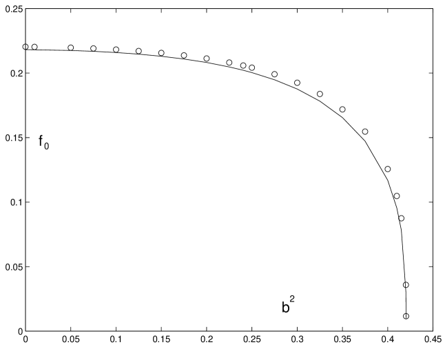
Figure 1: Critical point $f_{0}^{(2)}$ (open circles) and $f_{0}^{(3)}$ (continuous line) as a function of $b^{2}$

To illustrate the convergence of the zero locations $h_{n}$ and also how a good approximation the asymptotic (7.4) gives even for $h_{1}$, we collect some related numbers in table 3. The column $h_{1}^{\text{(as)}}$ corresponds to $n=1$ in (7.4) with $f_{0}=f_{0}^{(2)}$ from table 2. The value of $h_{0}^{\text{(exact)}}$ is taken at $b^{2}=0.4$ from the exact matrix model results (see next section) and at $b^{2}=0$ as the best TCS fit of [21].

$b^{2}$	$h_{0}^{(2)}$	$h_{0}^{(3)}$	$h_{0}^{(4)}$	$h_{0}^{\text{(exact)}}$	$h_{1}^{\text{(as)}}$	$h_{1}^{(3)}$	$h_{1}^{(4)}$
$0.00$	$2.42697$	$2.43068$	$2.43069$	$2.43069$	$-12.2410$	$-11.7540$	$-11.7667$
$0.01$	$2.44074$	$2.44446$			$-12.1991$	$-11.7193$
$0.05$	$2.50261$	$2.50648$			$-12.0120$	$-11.5656$
$0.10$	$2.60000$	$2.60444$			$-11.7880$	$-11.3549$
$0.15$	$2.73096$	$2.73652$			$-11.5990$	$-11.1519$
$0.1974$	$2.90514$	$2.91258$	$2.91264$		$-11.4909$	$-11.0075$	$-11.0267$
$0.20$	$2.91685$	$2.92443$			$-11.4880$	$-11.0020$
$0.2404$	$3.13562$	$3.14598$	$3.14606$		$-11.5099$	$-10.9730$	$-10.9928$
$0.25$	$3.20130$	$3.21256$			$-11.5386$	$-10.9867$
$0.30$	$3.69093$	$3.70962$			$-11.9506$	$-11.2907$
$0.35$	$4.74483$	$4.78283$			$-13.3915$	$-12.5134$
$0.40$	$9.22903$	$9.38245$	$9.38349$	$9.38350$	$-21.1991$	$-19.3580$	$-19.3879$

Table 3: Positions of first two zeros of $h(z)$ at different approximations

To summarize, using only three first coefficients of the power series in $z(h)$ we have restored to an impressive accuracy the free energy $f_{0}^{(3)}$ and also the first two zeros $h_{0}^{(3)}$ and $h_{1}^{(3)}$, the subsequent being given in this approximation by the asymptotic formula (7.4). With this data we can approximately calculate the next perturbative coefficients through the sum rules similar to (7.10). Such estimate $z_{4}^{\text{(sum)}}$ for the four point coefficient are quoted in the last column of table 1. These “extrapolated” numbers are compared with the actual ones where the last are available, i.e., at the classical point [21], the minimal gravity point $b^{2}=0.4$ and, in addition, at two special values of $b^{2}$ where the integral in the forth line of (4.39) is somewhat simpler and can be carried out (see in sect 11). The comparison is mainly to check the consistency of the four-point integrals with the expected analytic structure. Another reason is to estimate the numerical precision to be achieved in the four-point integration of (4.39) in order to add new information to the analytic-numeric data. The requirements to any numeric implementations turn out to be rather high (in most cases not less then 5–6 decimal digits of precision is needed).

9 “Integrable” point $b^{2}=2/5$

Point $b^{2}=2/5$ corresponds to $c_{\text{sp}}=0$, i.e., no spectator matter. The matter content of the critical (unperturbed) gravity is exhausted by a single minimal CFT model ($\mathcal{M}_{2/5}$ in the present case). This situation is called the “minimal gravity”. There are many reasons to believe that the minimal gravity is solvable, at least in its “topological” aspects. Namely, all (or at least large classes of) integrated multipoint correlation numbers are in principle calculable. The legend is that some versions of perturbed minimal gravity, to the utmost radical version all possible perturbations, are related to certain solvable matrix models [12] (more precisely, the classes of their critical behavior). Anyhow, in many cases this folklore can be promoted to specific statements and our problem of the perturbed minimal Yang-Lee gravity is among them.

The scaling function $Z_{\text{t}}(x,t)$, which describes the scaling region near the tricritical point of the one matrix model (at the planar limit corresponding to the spherical topology), is determined explicitly as

$$\frac{\partial^{2}}{\partial x^{2}}Z_{\text{t}}(x,t)=u(x,t)$$ (9.1)

through a solution $u(x,t)$ of the following simple algebraic equation

$$x=u^{3}-tu$$ (9.2)

In ref.[22] this scaling region has been identified with the perturbed critical $b^{2}=2/5$ minimal gravity, parameters $t$ and $x$ playing the role of the cosmological constant and $\varphi$-perturbation coupling respectively. Of course, this identification doesn’t fix the overall scale neither of the partition function (9.1) itself nor of the coupling constants. Thus, we have to identify $t$ and $x$ with $\mu$ and $\lambda$ and the spherical partition function (3.3) $Z_{\text{t}}(x,t)$ up to certain normalization constants.

Equations (9.1) and (9.2) result in the following expansion

$$Z_{\text{t}}(x,t) =t^{7/2}\sum_{n=0}^{\infty}\frac{1}{2}\frac{\Gamma(3n/2-7/2)}{n!\Gamma(n/2-1/2)}\left(\frac{x}{t^{3/2}}\right)^{n}$$ (9.3)

$$=Z_{\text{t}}(0,t)\left(1-\frac{105}{16}\left(\frac{x}{t^{3/2}}\right)+\frac{105}{8}\left(\frac{x}{t^{3/2}}\right)^{2}-\frac{35}{16}\left(\frac{x}{t^{3/2}}\right)^{3}+\ldots\right)$$

The linear in $x$ term is regular and therefore cannot be described unambiguously in the field theoretic context. In particular, this term doesn’t contribute to the fixed area partition function below. Hence we do not pay much attention to this term and instead compare the next terms with the perturbative coefficients (4.39). The $x^{2}$ term leads to the relation

$$\frac{x}{t^{3/2}}=\frac{\lambda l_{\text{eg}}}{(\pi\mu)^{3/2}}$$ (9.4)

which is also consistent with the $x^{3}$ term. Here

$$l_{\text{eg}}=\frac{\gamma^{1/2}(4/5)}{4\gamma(2/5)}=0.0845223\ldots$$ (9.5)

Also the singular point in $t$ is determined from (9.2) and (9.4)

$$\mu_{\text{c}}=\frac{3}{\pi}\left(\frac{l_{\text{eg}}}{2}\right)^{2/3}=0.11585962159187$$ (9.6)

This is the number quoted as $f_{0}^{\text{(exact)}}$ in the table 2.

Neglecting the overall normalization of the partition function, which in any case doesn’t enter the fixed area scaling function $z(h)$, we are in the position to write the latter explicitly. The coefficients in (4.43) are

$$z_{n}=-\frac{2\sqrt{\pi}(-l_{\text{eg}})^{n}}{n!\Gamma(n/2-1/2)}$$ (9.7)

Numerically

$$z_{2} =-l_{\text{eg}}^{2}=-0.00714401$$

$$z_{3} =\frac{\sqrt{\pi}}{3}l_{\text{eg}}^{3}=0.000356752$$ (9.8)

$$z_{4} =-\frac{1}{6}l_{\text{eg}}^{4}=-8.50615\ldots\times 10^{-6}$$

$$\ldots$$

The last number has been used in the previous section for the numerical analysis.

The following integral representation

$$z(h)=-\frac{2}{\sqrt{\pi}}\int_{\uparrow}y^{2}dy\exp\left(y^{2}+\frac{l_{\text{eg}}h}{y}\right)$$ (9.9)

where the integration is parallel to the imaginary axis and goes to the right from the singularity at $y=0$.

In fig.2 exact scaling function (9.9) is plotted. For comparison we present, without any comments, the numbers obtained by the order 3 (i.e., first three coefficients $z_{1}$, $z_{2}$ and $z_{3}$ are used in the analysis) analytic-numeric procedure of sect.8.

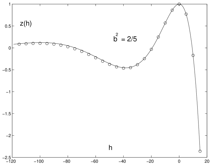
Figure 2: Continuous line: exact function $z(h)$ as defined by (9.9). Open circles: the canonical product over the zeros recovered from $z_{2}$ and $z_{3}$ through the analytic-numeric procedure

It is worth mentioning that the family of gravitational Yang-Lee models $0\leq b^{2}\leq b_{\text{c}}^{2}$ contains another interesting point $b^{2}=0.3$, where it can be reduced to the minimal gravity and therefore there are all reasons to expect the model to be solvable. At this point $c_{\text{sp}}=-22/5$ and the model can be thought of as two independent Yang-Lee models, one is perturbed while the other remains conformal (spectator). So far nothing special, one can make many similar combinations of minimal matter models constructing different theories of gravity, most of them being non-solvable (or non-integrable, in a wide sense). Combination $\mathcal{M}_{2/5}\oplus\mathcal{M}_{2/5}$ is exceptional, because it admits an alternative description in terms of single minimal model $\mathcal{M}_{3/10}$ (central charge $-44/5$) [23]. The table of degenerate dimensions of this model

$$2$$

(9.10)

includes the fields $\Phi_{1,5}$ and $\Phi_{2,5}$ of dimension $-1/5$. In the non-diagonal ($D$-series) version of this minimal model certain combination of these operators is interpreted as $\varphi$ acting only inside one of the constituent $\mathcal{M}_{2/5}$ models. It is natural to expect that such perturbed minimal gravity can be related to an appropriate matrix model, and therefore is solvable. The point seems to merit further study.

10 Four-point integral

Relative success of the numerical program of sect.8 makes it tempting to improve the approximation by involving the next four-order term $z_{4}$. This coefficient is related to the four-point correlation number. In the framework of Liouville gravity it requires an integration over moduli (4.4) of the product of the matter and the Liouville four-point functions, as in the last line of eq.(4.39). In the fixed area context it is more natural to use the fixed area Liouville four-point function

$$G_{\text{L}}^{(A=\pi)}(x,\bar{x})=\frac{\left.G_{\text{L}}(x,\bar{x})\right|_{\pi\mu=1}}{\Gamma(4gb^{-1}-Qb^{-1})}$$ (10.1)

The fixed area term is rewritten as

$$z_{4}=\frac{\mathcal{I}(b)}{24(2\pi)^{4}bZ_{\text{L}}^{(A=\pi)}}$$ (10.2)

where, as usual

$$Z_{\text{L}}^{(A=\pi)}=\frac{\gamma^{Q/b}(b^{2})\Gamma(2-b^{2})}{\pi^{3}b^{3}\Gamma(b^{2})\Gamma(b^{-2})}$$ (10.3)

and

$$\mathcal{I}(b)=b\int G_{\text{YL}}(x,\bar{x})G_{\text{L}}^{(A=\pi)}(x,\bar{x})d^{2}x$$ (10.4)

with $G_{\text{YL}}(x,\bar{x})$ from eq.(6.3).

In general the Liouville four-point function admits the block representation (4.27), which reads in our symmetric case as

$$\left.G_{\text{L}}(x,\bar{x})\right|_{\pi\mu=1}=\mathcal{R}_{g}\int^{\prime}\frac{dP}{4\pi}r_{g}(P)\mathcal{F}_{P}\left(\left.\begin{array}[c]{cc}\Delta_{g}&\Delta_{g}\\ \Delta_{g}&\Delta_{g}\end{array}\right|x\right)\mathcal{F}_{P}\left(\left.\begin{array}[c]{cc}\Delta_{g}&\Delta_{g}\\ \Delta_{g}&\Delta_{g}\end{array}\right|\bar{x}\right)$$ (10.5)

Here the overall factor $\mathcal{R}_{g}$ reads

$$\mathcal{R}_{g}=\left(\gamma(b^{2})b^{2-2b^{2}}\right)^{(Q-4g)/b}\frac{\Upsilon_{b}^{4}(b)\Upsilon_{b}^{4}(2g)}{\pi^{2}\Upsilon_{b}^{4}(2g-Q/2)}$$ (10.6)

while the function

$$r_{g}(P)=\frac{\pi^{2}\Upsilon_{b}(2iP)\Upsilon_{b}(-2iP)\Upsilon_{b}^{4}(2g-Q/2)}{\Upsilon_{b}^{2}(b)\Upsilon_{b}^{2}(2g-Q/2-iP)\Upsilon_{b}^{2}(2g-Q/2+iP)\Upsilon_{b}^{2}(Q/2-iP)\Upsilon_{b}^{2}(Q/2+iP)}$$ (10.7)

admits the following integral representation (convergent at $g>Q/4$)

$$r_{g}(P)=\sinh 2\pi b^{-1}P\sinh 2\pi bP\exp\left(-8\int_{0}^{\infty}\frac{dt}{t}\frac{\sin^{2}Pt\left(\cosh^{2}(Q-2g)t-e^{-Qt}\cos^{2}Pt\right)}{\sinh bt\sinh b^{-1}t}\right)$$ (10.8)

Integral (10.5) should be taken literally if $Q/2>g>Q/4$, otherwise there are additional “discrete” terms due to the singularities of the integrand [15]. The prime near the integral sign in (10.5) indicates this subtlety.

Apparently the form $G_{\text{YL}}(x,\bar{x})G_{\text{L}}^{(A=\pi)}(x,\bar{x})d^{2}x$ in the integral (10.4) is invariant under the group of $6$ modular transformations

$$R :x\rightarrow 1-x$$

$$I :x\rightarrow 1/x$$

$$RI :x\rightarrow 1/(1-x)$$ (10.9)

$$IR :x\rightarrow 1-1/x$$

$$IRI=RIR :x\rightarrow x/(x-1)$$

Therefore the integration in (10.4) can be restricted to its fundamental domain $\mathbf{F=}\{{\operatorname*{Re}}x<1/2;\;\left|1-x\right|<1\}$ (see fig.3)

$$\mathcal{I}(b)=6b\int_{\mathbf{F}}G_{\text{YL}}(x,\bar{x})G_{\text{L}}^{(A=\pi)}(x,\bar{x})d^{2}x$$ (10.10)

Figure 3: Fundamental region of the modular group (10.9) and the action of its elements.

Evaluation of integrals in (10.4) or (10.10), even numerical, presents certain technical difficulties. They are mostly related to the complicated nature of the Liouville four point function. Expression (10.5) involves additional integration in (10.8) to evaluate the special functions. This makes the integral in (10.10) three-fold. In addition the general conformal block entering (10.5) is usually known only as a power series in $x$, its evaluation requiring certain recursive procedure [24].

There is another representation of integral (10.4) which takes advantage of the holomorphic factorization in each term of the matter and Liouville block decompositions (6.3) and (4.27) respectively. It is based on the following simple calculation. Consider the integral

$$\mathcal{I}=\int G(x,\bar{x})d^{2}x$$ (10.11)

where $G(x,\bar{x})$ is singular at $x=0$, $1$ and $\infty$ only and admits the representation

$$G(x,\bar{x})=\sum_{i}A_{i}\mathcal{F}_{i}(x)\mathcal{F}_{i}(\bar{x})$$ (10.12)

(the sum over $i$ might be as well an integral over a continuous spectrum or both) with some coefficients $A_{i}$. The holomorphic “blocks” are singular at $x=0$, where $\mathcal{F}_{i}(x)\sim x^{\Delta_{i}}$, and also at $x=1$ and $x=\infty$, the combination (10.12) being arranged so as to form a single-valued function of $x$. Straightforward application of the Stokes theorem gives

$$\mathcal{I}=\frac{1}{2i}\sum_{i}A_{i}I_{i}J_{i}$$ (10.13)

where

$$I_{i} =\int_{0}^{1}\mathcal{F}_{i}(x)dx$$ (10.14)

$$J_{i} =\int_{C}\mathcal{F}_{i}(x)dx$$

and the contour $C$ goes from $-\infty$ to $-\infty$ around $x=0$ counterclockwise. If, in addition the integrand in (10.11) is symmetric with respect to the modular group (10.9), equation (10.13) is reduced to

$$\mathcal{I}=-\sum_{i}\sin(\pi\Delta_{i})A_{i}I_{i}^{2}$$ (10.15)

In our particular problem this identity reads (again up to certain discrete terms at $g<Q/4$)

$$I(b)=-b\mathcal{R}_{g}\int^{\prime}\frac{dP}{4\pi}r_{g}(P)\left(\sin\pi\Delta_{P}I_{I}^{2}(P)-\kappa^{2}\sin\pi(\Delta_{P}-1/5)I_{\varphi}^{2}(P)\right)$$ (10.16)

where

$$I_{I}(P) =\int_{0}^{1}\mathcal{F}_{I}(x)\mathcal{F}_{P}\left(\left.\begin{array}[c]{cc}\Delta_{g}&\Delta_{g}\\ \Delta_{g}&\Delta_{g}\end{array}\right|x\right)dx$$ (10.19)

$$I_{\varphi}(P) =\int_{0}^{1}\mathcal{F}_{\varphi}(x)\mathcal{F}_{P}\left(\left.\begin{array}[c]{cc}\Delta_{g}&\Delta_{g}\\ \Delta_{g}&\Delta_{g}\end{array}\right|x\right)dx$$ (10.22)

$\mathcal{F}_{I}(x)$ and $\mathcal{F}_{\varphi}(x)$ are from eq.(6.4).

Expression (10.16) has an obvious advantage compared with the form (10.10), since it involves one integration less. However, evaluation of the line integrals (10.19) requires the Liouville block to be computed to the required accuracy up to the upper limit $x=1$. For a function known mainly through its power series this makes an additional problem. On the other hand, representation (10.10) contains only the blocks with $\left|x\right|<\sqrt{3}/2$, where the convergence of the block power series is still reasonable. To conclude, it is difficult to say in advance which one of these two representations is better for numerical work. In the next section we take two special values of $b^{2}$ where the Liouville correlation function can be found in closed form. The Liouville blocks explicitly known make formula (10.16) very effective and accurate. This will allow us to estimate the numerical precision of the direct integration in (10.10).

11 Special $b^{2}$

Liouville correlation function $\left\langle e^{2a_{1}\phi(x_{1})}\ldots e^{2a_{N}\phi(x_{N})}\right\rangle_{\text{L}}$ develop poles if its parameters $a_{i}$ satisfy certain relations. Following A.Polyakov [25] we will call them the “on-mass-shell” conditions and the corresponding correlations the “resonant” ones. The simplest on-mass-shell condition reads for $a=\sum_{i=1}^{N}a_{i}$

$$a=Q-nb$$ (11.1)

with $n$ non-negative integer. It can be easily traced to the divergency in the integration over the “zero mode” of the Liouville field [26, 27]. The residues in the resonant poles (11.1) can be “naively” red off from the Liouville Lagrangian (2.2)

$$\left\langle e^{2a_{1}\phi(x_{1})}\ldots e^{2a_{N}\phi(x_{N})}\right\rangle_{\text{L}}\sim\frac{(-\mu)^{n}}{n!}\frac{\mathcal{G}_{n}(a_{1},\ldots,a_{N})}{a-Q+nb}$$ (11.2)

where

$$\mathcal{G}_{n}(a_{1},\ldots,a_{n})=\int\left\langle e^{2a_{1}\phi(x_{1})}\ldots e^{2a_{n}\phi(x_{n})}\prod_{k=1}^{n}e^{2b\phi(y_{k})}d^{2}y_{k}\right\rangle$$ (11.3)

and the expectation value in the right hand side is over free massless boson without the zero mode.

In particular in the four-point case the simplest $n=0$ resonance doesn’t require any integrals in the right hand side and the “reduced” four point function of (4.21) takes the form

$$G_{\text{L}}\left(\left.\begin{array}[c]{cc}a_{1}&a_{3}\\ a_{2}&a_{4}\end{array}\right|x,\bar{x}\right)=\frac{\mathcal{G}_{0}(x,\bar{x})}{a-Q}$$ (11.4)

where

$$\mathcal{G}_{0}(x,\bar{x})=(x\bar{x})^{-2a_{1}a_{2}}((1-x)(1-\bar{x}))^{-2a_{1}a_{3}}$$ (11.5)

Similarly, the next resonance at $a=Q-b$ is controlled by a single “screening integral” in (11.3)

$$\mathcal{G}_{1}(x,\bar{x})=\frac{1}{(x\bar{x})^{2a_{1}a_{2}}((1-x)(1-\bar{x}))^{2a_{1}a_{3}}}\int\frac{d^{2}y}{(y\bar{y})^{2a_{2}b}((1-y)(1-\bar{y}))^{2a_{3}b}((x-y)(\bar{x}-\bar{y}))^{2a_{1}b}}$$ (11.6)

It admits the two-term holomorphic decomposition

$$\mathcal{G}_{1}(x,\bar{x})=k_{1}\mathcal{F}_{1}(x)\mathcal{F}_{1}(\bar{x})+k_{2}\mathcal{F}_{2}(x)\mathcal{F}_{2}(\bar{x})$$ (11.7)

where

$$k_{1} =\frac{\pi\gamma(1-2a_{2}b-2a_{1}b)\gamma(1-2a_{3}b)}{\gamma(2-2a_{2}b-2a_{3}b-2a_{1}b)}$$ (11.8)

$$k_{2} =\frac{\pi\gamma(1-2a_{2}b)\gamma(1-2a_{1}b)}{\gamma(2-2a_{1}b-2a_{2}b)}$$

and

$$\mathcal{F}_{1}(x) =x^{-2a_{1}a_{2}}(1-x)^{-2a_{1}a_{3}}{}{}_{2}F_{1}(2a_{1}b+2a_{2}b+2a_{3}b-1,2a_{1}b,2a_{1}b+2a_{2}b,x)$$ (11.9)

$$\mathcal{F}_{2}(x) =x^{1-2a_{2}b-2a_{1}b-2a_{1}a_{2}}(1-x)^{-2a_{1}a_{3}}{}_{2}F_{1}(1-2a_{2}b,2a_{3}b,2-2a_{1}b-2a_{2}b,x)$$

To check the consistency of the resonance condition in LFT, in Appendix B we rederive the residues (11.5) and (11.7) from the general four-point expression (4.27).

From eq.(10.1) it is clear that the poles at (11.1) are canceled out in the fixed area correlation functions and the finite parts

$$\left\langle e^{2a_{1}\phi(x_{1})}\ldots e^{2a_{N}\phi(x_{N})}\right\rangle_{\text{L}}^{(A)}=b^{-1}A^{-n}\mathcal{G}_{n}(a_{1},\ldots,a_{N})$$ (11.10)

are expressed through (11.3). In our four-point case this means that (10.4) reads

$$\mathcal{I}(b_{n})=\frac{1}{\pi^{n}}\int G_{\text{YL}}(x,\bar{x})\mathcal{G}_{n}(x,\bar{x})d^{2}x$$ (11.11)

1. The first resonant point $n=0$ appears in our particular problem (11.4) at $b=b_{0}$

$$b_{0}^{2}=\frac{11-4\sqrt{6}}{5}=0.240408205773\ldots$$ (11.12)

At this point the Liouville dressing parameter $g^{2}=2/5$ so that

$$\mathcal{G}_{0}(x,\bar{x})=\left[x\bar{x}(1-x)(1-\bar{x})\right]^{-4/5}$$ (11.13)

Hence

$$\mathcal{I}(b_{0})=\int\frac{\mathcal{F}_{I}(x)\mathcal{F}_{I}(\bar{x})-\kappa^{2}\mathcal{F}_{\varphi}(x)\mathcal{F}_{\varphi}(\bar{x})}{\left[x\bar{x}(1-x)(1-\bar{x})\right]^{4/5}}d^{2}x$$ (11.14)

Direct integration over the fundamental region gives (NIntegrate of Mathematica 3.0)

$$\mathcal{I}(b_{0})=6\int_{\mathbf{F}}\frac{G_{\text{YL}}(x,\bar{x})}{\left[x\bar{x}(1-x)(1-\bar{x})\right]^{4/5}}d^{2}x=-59.9029678...$$ (11.15)

The reduction formula (10.15) gives in this case two terms

$$\mathcal{I}(b_{0})=\sin\frac{2\pi}{5}I_{1}^{2}-\kappa^{2}\sin\frac{3\pi}{5}I_{2}^{2}$$ (11.16)

Here both contour integrals are carried out explicitly

$$I_{1} ={\displaystyle\int_{0}^{1}}\frac{F(2/5,3/5,6/5,t)}{t^{2/5}(1-t)^{3/5}}dt=\frac{2^{4/5}\pi(\sqrt{5}-1)\Gamma^{2}(6/5)}{\Gamma(7/10)\Gamma(9/10)\Gamma(9/5)}$$ (11.17)

$$I_{2} ={\displaystyle\int_{0}^{1}}\frac{F(1/5,2/5,4/5,t)}{t^{3/5}(1-t)^{3/5}}dt=\frac{\sqrt{\pi}\Gamma(1/5)}{2^{2/5}\Gamma(7/10)}$$

and (11.16) sums up to

$$\mathcal{I}(b_{0})=-\frac{\pi}{50}\gamma^{5}(1/5)=-59.9030606...$$ (11.18)

Finally

$$z_{4}=\frac{\mathcal{I}(b_{0})}{384b\pi^{4}Z_{\text{L}}^{(A)}}=-0.00102377123\ldots$$ (11.19)

is the number used in sect.8 for this special point.

2. The second resonant point $n=1$ corresponds to

$$b_{1}^{2} =\frac{15}{76}=0.197368421\ldots$$ (11.20)

$$g^{2} =\frac{19}{60}$$

Notice that $gb=1/4$ and thus the integral (11.6) reads

$$\mathcal{G}_{1}(x,\bar{x})=\frac{1}{[(x\bar{x})(1-x)(1-\bar{x})]^{2g^{2}}}\int\frac{d^{2}y}{\left[y\bar{y}(1-y)(1-\bar{y})(x-y)(\bar{x}-\bar{y})\right]^{1/2}}$$ (11.21)

This fact is general for the $n=1$ resonance in the symmetric case, for $\sum_{i=1}^{4}a_{i}=4g=Q-b$. The integral is a degenerate case of (11.6). The result is recovered at the limit $2a_{i}b\rightarrow 1/2$ in (11.7)

$$\mathcal{G}_{1}(x,\bar{x})=\frac{4\left[K(x)K(1-\bar{x})+K(1-x)K(\bar{x})\right]}{[x\bar{x}(1-x)(1-\bar{x})]^{19/30}}$$ (11.22)

in terms of the elliptic integral of the first kind

$$K(x)=\frac{1}{2}\int_{0}^{1}\frac{dy}{\sqrt{y(1-y)(1-xy)}}$$ (11.23)

Collecting all together we find

$$\mathcal{I}(b_{1})=\frac{1}{\pi}\int G_{\text{YL}}(x,\bar{x})\mathcal{G}_{1}(x,\bar{x})d^{2}x$$ (11.24)

Direct integration gives with Mathematica 3.0

$$\mathcal{I}(b_{1})=\frac{6}{\pi}\int_{\mathbf{F}}G_{\text{YL}}(x,\bar{x})\mathcal{G}_{1}(x,\bar{x})d^{2}x=-302.01932532722\ldots$$ (11.25)

The reduction formula (10.15) doesn’t apply here directly due to the degeneration. It is more convenient to reduce first a more general integral with (11.6) as the Liouville part. Then the limit $2a_{i}b\rightarrow 1/2$ reveals

$$\mathcal{I}(b_{1})=\frac{8}{\pi}\left(\sin\frac{7\pi}{30}I_{I}J_{I}-2\kappa^{2}\sin\frac{13\pi}{30}I_{\varphi}J_{\varphi}\right)$$ (11.26)

where

$$I_{I,\varphi}=\int_{0}^{1}\frac{\mathcal{F}_{I,\varphi}(x)K(x)}{(x(1-x))^{19/30}}dx\;;\;\;\;J_{I,\varphi}=\int_{0}^{1}\frac{\mathcal{F}_{I,\varphi}(x)K(1-x)}{(x(1-x))^{19/30}}dx$$ (11.27)

In numbers

$$\mathcal{I}(b_{1})=-302.01932904124\ldots$$ (11.28)

and

$$z_{4}=\frac{\mathcal{I}(b_{1})}{384b\pi^{4}Z_{\text{L}}^{(A)}}=-0.0014386452412875\ldots$$ (11.29)

Reduction formula gives more accurate numbers. This permits to estimate the precision of the direct integration. In the above two examples it varies between 5–8 decimal digits. The accuracy of the direct integration is determined mainly by the singular behavior near $x=0$ in the fundamental region. Thus, for $b^{2}$ closer to the critical point $b_{\text{c}}^{2}$, where the “tachyon” divergence appears, the direct integration is hardly expected to give a good approximation.

The following remark is in order here. At the fixed area picture the $n$-th resonance (11.1) correlation function gives in the partition function a contribution proportional to the negative integer powers $A^{-n}$. The transform to the grand partition function (3.6) results in the terms containing $\mu^{n}\log\mu$. This is quite usual phenomenon in the field theory: integer powers of the coupling constant are usually decorated by logarithm. Otherwise these terms are regular in $\mu$, i.e. contact (from the common point of view they are out of the field theory scope). On the other hand, the analysis of the critical behavior in solvable matrix models is similar to that in the mean field, or Ginzburg-Landau theory, and thus deals only with the algebraic functions where there is no place for the logarithms. This might give an impression that the mean field like pattern of critical behavior is common for the statistical systems interacting with quantum gravity. We have seen in the above examples that this is certainly not the case and might be true at most for the systems related to the solvable matrix models.

12 Discussion

I think that the main lesson to be learned from those rather random calculations presented above is that the perturbed Liouville gravity based on the existing LFT constructions is indeed a consistent tool to treat the standard problems in 2D gravity. Although at present it cannot yet give any exact description even in the problems known to be exactly solvable, sometimes it works equally well in the situations which are not covered by the solvable matrix models and therefore most probably are not exactly solvable. On the other hand, non-solvable gravities certainly exist and might be observed e.g., as critical points of non-solvable random lattice statistical systems. More generally, it is likely too hasty to claim the field theory obsolete, substituted by the matrix models (or whatsoever).

As for the “spectator matter” appeared in an apparently artificial way, there are many practical ways to introduce such content in the statistical models of lattice gravity. The simplest way is to add a $D$-dimensional free massless lattice boson (without zero mode) which doesn’t interact with other matter degrees of freedom and contributes simply as an extra weight factor $\det^{-D/2}\Delta_{\text{lat}}$, where $\Delta_{\text{lat}}$ is the discrete Laplace operator of the graph. Apparently this parameter $D=c_{\text{sp}}$ can be as well made continuous. Not to talk about the obvious idea of putting several extra non-interacting spin-like degrees of freedom and tuning them to their critical points. As far as I understand, all these situations can be studied either through the extrapolation of the finite lattice ensembles or in the Monte-Carlo simulations.

Acknowledgments

My special gratitude is to Galina Gritsenko for her permanent moral support during all these years of gradual composing the manuscript. The writing has been finished while the author stayed with a visit at Kawai Theoretical Laboratory of RIKEN. The hospitality, stimulating scientific atmosphere of the group and discussions with Y.Ishimoto are highly acknowledged. I am also obliged to Alexander Zamolodchikov for his authentic and intelligent interest to the work. Different parts of this study has been reported many times at different seminars. I thank all my friends and colleagues for their sincere attempts to understand the motivations to mess around with this ugly non-integrable pet of mine. The work was supported by the European Committee under contract EUCLID HRPN-CT-2002-00325.

Appendix A Series analysis

Suppose that the order $\rho$ of $z(h)$ is less then $1$ and therefore

$$z(h)=\prod_{n=0}^{\infty}\left(1-\frac{h}{h_{n}}\right)=\prod_{n=0}^{N-2}\left(1-\frac{h}{h_{n}}\right)\exp\left(-\sum_{k=1}^{\infty}r_{k}(-h)^{k}\right)$$ (A.1)

where $N$ is any natural number (for our particular problem $N\geq 2$) and

$$r_{k}=\frac{(-1)^{k}}{k}\sum_{N-1}^{\infty}\frac{1}{h_{n}^{k}}$$ (A.2)

Thus

$$P_{N}(h)=z(h)\exp\left(\sum_{k=1}^{\infty}r_{k}(-h)^{k}\right)$$ (A.3)

is a polynomial of order $N-1$ with zeros at $h_{n}$, $n=0,1,\ldots,N-2$ (we have introduced certain unnecessary minus signs in the notations for further convenience).

This set of trivial identities gives rise to the following algorithm for the problem of sect.7 : solve first truncated $N$ sum rules (7.10) for $Y$ and first $N-1$ zeros $h_{0},\ldots,h_{N-2}$ given the first $N$ non-trivial coefficients $z_{n}$ in

$$z(h)=\sum_{n=0}^{\infty}z_{n}(-h)^{n}$$ (A.4)

The truncation means that all terms in the r.h.s. of (7.10) with $n>N-2$ are replaced by the corresponding asymptotic values (7.4). In our present algebraic context the coefficients $r_{k}$ in (A.2) are taken as

$$r_{k}=d_{k}Y^{k}$$ (A.5)

with some known numbers $d_{k}$ (in our actual context $d_{k}=k^{-1}\zeta(k/\rho,N-1-\delta)$). Then

$$\exp\left(\sum_{k=1}^{\infty}r_{k}(-h)^{k}\right)=\sum_{n=0}^{\infty}a_{n}(-hY)^{n}$$ (A.6)

is a regular series in $hY$ with known coefficients

$$a_{n}=\sum_{k_{1}+\ldots+k_{l}=n}\prod_{l}\frac{d_{l}^{k_{l}}}{k_{l}!}$$ (A.7)

The coefficient of order $N$ in (A.3) is zero. This gives the algebraic equation for $Y$

$$Q_{N}(Y)=\sum_{k=0}^{N}a_{k}z_{N-k}Y^{k}=0$$ (A.8)

Once $Y$ is found as a suitable solution to this equation, the $N-1$ roots of the polynomial are found as the roots of the polynomial

$$\sum_{n=0}^{N-1}Q_{n}(Y)(-h)^{n}=0$$ (A.9)

where

$$Q_{n}(Y)=\sum_{k=0}^{n}a_{k}z_{n-k}Y^{k}$$ (A.10)

Appendix B Resonant Liouville correlations

Consider the general Liouville four-point function (4.27)

$$\ \int_{\uparrow}\frac{dc}{4\pi i}C_{\text{L}}\left(a_{1},a_{2},c\right)C_{\text{L}}\left(Q-c,a_{3},a_{4}\right)\mathcal{F}\left(\left.\begin{array}[c]{cc}\Delta_{1}&\Delta_{3}\\ \Delta_{2}&\Delta_{4}\end{array}\right|\Delta_{c};x\right)\mathcal{F}\left(\left.\begin{array}[c]{cc}\Delta_{1}&\Delta_{3}\\ \Delta_{2}&\Delta_{4}\end{array}\right|\Delta_{c};\bar{x}\right)$$

in the vicinity of the first resonant point

$$a_{1}+a_{2}+a_{3}+a_{4}-Q=\epsilon$$ (B.1)

with $\epsilon$ small. Due to the denominators $\Upsilon_{b}(a_{1}+a_{2}-c)$ and $\Upsilon_{b}(a_{3}+a_{4}+c-Q)$ in

$$C_{\text{L}}(a_{1},a_{2},c)C_{\text{L}}(Q-c,a_{3},a_{4})=\left(\pi\mu\gamma(b^{2})b^{2-2b^{2}}\right)^{(Q-a_{1}-a_{2}-a_{3}-a_{4})/b}\times$$

$$\ \ \ \ \ \frac{\Upsilon_{b}(b)\Upsilon_{b}(2a_{1})\Upsilon_{b}(2a_{2})\Upsilon_{b}(2c)}{\Upsilon_{b}(a_{1}+a_{2}+c-Q)\Upsilon_{b}(a_{1}+a_{2}-c)\Upsilon_{b}(c+a_{1}-a_{2})\Upsilon_{b}(c+a_{2}-a_{1})}\times$$ (B.2)

$$\ \ \ \ \ \frac{\Upsilon_{b}(b)\Upsilon_{b}(2a_{3})\Upsilon_{b}(2a_{4})\Upsilon_{b}(2Q-2c)}{\Upsilon_{b}(a_{3}+a_{4}+c-Q)\Upsilon_{b}(a_{3}+a_{4}-c)\Upsilon_{b}(c+a_{3}-a_{4})\Upsilon_{b}(c+a_{4}-a_{3})}$$

there are close poles: at $c=$ $a_{1}+a_{2}-\epsilon$ to the left from the integration contour and at $c=a_{1}+a_{2}$ to the right. This pinch results in the singular contribution

$$\frac{1}{2\epsilon}\mathcal{F}\left(\left.\begin{array}[c]{cc}\Delta_{1}&\Delta_{3}\\ \Delta_{2}&\Delta_{4}\end{array}\right|\Delta_{a_{1}+a_{2}};x\right)\mathcal{F}\left(\left.\begin{array}[c]{cc}\Delta_{1}&\Delta_{3}\\ \Delta_{2}&\Delta_{4}\end{array}\right|\Delta_{a_{1}+a_{2}};\bar{x}\right)$$ (B.3)

All other multipliers in (B.2) cancel out in the residue. It is not a problem to verify that

$$\mathcal{F}\left(\left.\begin{array}[c]{cc}\Delta_{1}&\Delta_{3}\\ \Delta_{2}&\Delta_{4}\end{array}\right|\Delta_{a_{1}+a_{2}};x\right)=x^{-2a_{1}a_{2}}(1-x)^{-2a_{1}a_{3}}$$ (B.4)

A “mirror” contribution comes from the pinch at $c=Q-a_{1}-a_{2}$ provided by the $\Upsilon_{b}(a_{1}+a_{2}+c-Q)$ and $\Upsilon_{b}(a_{3}+a_{4}-c)$ denominators in (B.2). Its contribution is identical and we arrive at (11.5). Of course the same situation appears if one or more of $a_{i}$ in (B.1) are reflected, e.g., $a_{1}+a_{2}+a_{3}-a_{4}=\epsilon$ or $Q+a_{1}-a_{2}+a_{3}-a_{4}=\epsilon$. Then other pairs of $\Upsilon_{b}$-functions give rise to the singularity, which remains the same up to the expected reflection factors.

Let’s now take the second resonant point

$$a_{1}+a_{2}+a_{3}+a_{4}-Q=-b+\epsilon$$ (B.5)

The same pair of denominators $\Upsilon_{b}(a_{1}+a_{2}-c)$ and $\Upsilon_{b}(a_{3}+a_{4}+c-Q)$ in (B.2) produces two pairs of close poles at $c_{1}=$ $a_{1}+a_{2},\;a_{1}+a_{2}-\epsilon$ and $c_{2}=a_{1}+a_{2}+b,\;a_{1}+a_{2}+b-\epsilon$. The singular residues are

$$-\frac{\pi\mu}{2\epsilon}\frac{\gamma(1-2a_{1}b-2a_{2}b)}{\gamma(2a_{3}b)\gamma(2a_{4}b)}\mathcal{F}\left(\left.\begin{array}[c]{cc}\Delta_{1}&\Delta_{3}\\ \Delta_{2}&\Delta_{4}\end{array}\right|\Delta_{a_{1}+a_{2}};x\right)\mathcal{F}\left(\left.\begin{array}[c]{cc}\Delta_{1}&\Delta_{3}\\ \Delta_{2}&\Delta_{4}\end{array}\right|\Delta_{a_{1}+a_{2}};\bar{x}\right)$$ (B.6)

and

$$-\frac{\pi\mu}{2\epsilon}\frac{\gamma(1-2a_{3}b-2a_{3}b)}{\gamma(2a_{2}b)\gamma(2a_{1}b)}\mathcal{F}\left(\left.\begin{array}[c]{cc}\Delta_{1}&\Delta_{3}\\ \Delta_{2}&\Delta_{4}\end{array}\right|\Delta_{a_{1}+a_{2}+b};x\right)\mathcal{F}\left(\left.\begin{array}[c]{cc}\Delta_{1}&\Delta_{3}\\ \Delta_{2}&\Delta_{4}\end{array}\right|\Delta_{a_{1}+a_{2}+b};\bar{x}\right)$$ (B.7)

The “mirror” pair $\Upsilon_{b}(a_{1}+a_{2}+c-Q)$ and $\Upsilon_{b}(a_{3}+a_{4}-c)$ contributes identically (in fact, this is a general feature related to the symmetries of the integrand in (4.27)). The identities for the blocks

$$\mathcal{F}\left(\left.\begin{array}[c]{cc}\Delta_{1}&\Delta_{3}\\ \Delta_{2}&\Delta_{4}\end{array}\right|\Delta_{a_{1}+a_{2}};x\right)=$$ (B.10)

$$\ \ \ x^{-2a_{1}a_{2}}(1-x)^{-2a_{1}a_{3}}{}{}_{2}F_{1}(2a_{1}b+2a_{2}b+2a_{3}b-1,2a_{1}b,2a_{1}b+2a_{2}b,x)$$

and

$$\ \mathcal{F}\left(\left.\begin{array}[c]{cc}\Delta_{1}&\Delta_{3}\\ \Delta_{2}&\Delta_{4}\end{array}\right|\Delta_{a_{1}+a_{2}+b};x\right)=$$ (B.13)

$$\ \ \ x^{1-2a_{2}b-2a_{1}b-2a_{1}a_{2}}(1-x)^{-2a_{1}a_{3}}{}_{2}F_{1}(1-2a_{2}b,2a_{3}b,2-2a_{1}b-2a_{2}b,x)$$

bring us to eq.(11.7).

References

• [1] A.Polyakov. Quantum geometry of bosonic strings. Phys.Lett., B103 (1981) 207.
• [2] A.Belavin, A.Polyakov and A.Zamolodchikov. Infinite conformal symmetry in two-dimensional quantum field theory. Nucl.Phys., B241 (1984) 333.
• [3] T.Curtright and C.Thorn. Conformally invariant quantization of the Liouville theory. Phys.Rev.Lett., 48 (1982) 1309; E.Braaten, T.Curtright and C.Thorn. Quantum Backlund transformation for the Liouville theory. Phys.Lett. B118 (1982) 115; An exact operator solution of the quantum Liouville field theory. Ann.Phys., 147 (1983) 365.
• [4] E.D’Hoker and R.Jackiw. Liouville field theory. Phys.Rev., D26 (1982) 3517.
• [5] J.-L.Gervais and A.Neveu. Novel triangle relation and absence of tachyons in Liouville string field. Nucl.Phys., B238 (1984) 125; Green functions and scattering amplitudes in Liouville string field theory. Nucl.Phys., B238 (1984) 396; Nonstandard two-dimensional critical statistical models from Liouville. Nucl.Phys. B257[FS14] (1985) 59.
• [6] V. A. Kazakov. Bilocal regularization of models of random surfaces. Phys.Lett., B150 (1985) 282.
• [7] F. David. A model of random surfaces with nontrivial critical behavior. Nucl.Phys., B257 (1985) 543.
• [8] V.Kazakov, A.Migdal and I.Kostov. Critical properties of randomly triangulated planar random surfaces. Phys.Lett. B157 (1985) 295.
• [9] V.Knizhnik, A.Polyakov and A.Zamolodchikov. Fractal structure of 2–D quantum gravity. Mod.Phys.Lett., A3 (1988) 819.
• [10] F.David. Conformal field theories coupled to 2-D gravity in the conformal gauge. Mod. Phys.Lett., A3 (1988) 1651.
• [11] J.Distler and H.Kawai. Conformal field theory and 2-D quantum gravity or who’s afraid of Joseph Liouville? Nucl.Phys., B231 (1989) 509.
• [12] I.Klebanov. String theory in two dimensions. Lectures at ICTP Spring School on String Theory and Quantum Gravity. Trieste, April 1991, hep-th/9108019; P.Ginsparg and G.Moore. Lectures on 2D gravity and 2D string theory. TASI summer school, 1992, hep-th/9304011; P.Di Francesco, P.Ginsparg and J.Zinn-Justin. 2D Gravity and Random Matrices. Phys.Rep. 254 (1995) 1–133.
• [13] M.Douglas, I.Klebanov, D.Kutasov, J.Maldacena, E.Martinec and N.Seiberg. A new hat for the $c=1$ matrix model. hep-th/0307195; N.Seiberg and D.Shih. Branes, rings and matrix models in minimal (super)string theory. hep-th/0312170.
• [14] H.Dorn and H.-J.Otto. On correlation functions for non-critical strings with $c<1$ but $d>1$. Phys.Lett., B291 (1992) 39, hep-th/9206053; Two and three point functions in Liouville theory. Nucl.Phys., B429 (1994) 375, hep-th/9403141.
• [15] A.Zamolodchikov and Al.Zamolodchikov. Structure constants and conformal bootstrap in Liouville field theory. Nucl.Phys., B477 (1996) 577.
• [16] J.Cardy. Phys.Rev.Lett., 54 (1985) 1354;
• [17] J.Cardy and G.Mussardo. Phys.Lett., B225 (1989) 275.
• [18] Al.Zamolodchikov. Mass scale in sin-Gordon and its reductions. Int.J.Mod.Phys., A10 (1995) 115.
• [19] Al.Zamolodchikov. Thermodynamic Bethe ansatz in scaling three state Potts model and scaling Lee-Yang model. Nucl.Phys., B342 (1990) 695.
• [20] C.Destri and H.deVega. Nucl.Phys., B358 (1991) 251.
• [21] Al.Zamolodchikov. Scaling Lee-Yang model on a sphere. I: Partition function. JHEP 0207 (2002) 029; hep-th/0109078.
• [22] M.Staudacher. The Yang-Lee edge singularity on a dynamical planar random surface. Nucl.Phys., B336 (1990) 349.
• [23] A. B. Zamolodchikov. Vacuum Ward identities for higher genera. Nucl.Phys., B316 (1989) 573.
• [24] Al.Zamolodchikov. Conformal symmetry in two-dimensions: an explicit recurrence formula for the conformal partial wave amplitude. Commun.Math.Phys., 96 (1984) 419; Confomal symmetry in two-dimensional space: recursion representation of conformal block. Theor.Math.Phys., 73 (1987) 1088–1093.
• [25] A.Polyakov. Selftuning fields and resonant correlations in 2-d gravity. Mod.Phys.Lett. A6 (1991) 635 (also in NY Quarks, Symm.Str.1990: 241-252).
• [26] M.Goulian and M.Li. Correlation functions in Liouville theory. Phys.Rev.Lett., 66 (1991) 2051.
• [27] P.Di Francesco and D.Kutasov. Correlation functions in 2-D string theory. Phys.Lett. B261 (1991) 385.