Is Hilbert space discrete?

Abstract

We show that discretization of spacetime naturally suggests discretization of Hilbert space itself. Specifically, in a universe with a minimal length (for example, due to quantum gravity), no experiment can exclude the possibility that Hilbert space is discrete. We give some simple examples involving qubits and the Schrodinger wavefunction, and discuss implications for quantum information and quantum gravity.

today

There are many indications that spacetime may be discrete rather than continuous minlength . For example, metric fluctuations due to quantum gravity might preclude any notion of distances less than of order the Planck length $l_{P}$. Recent work CGH has shown that no macroscopic experiment can be sensitive to discreteness of position on scales less than the Planck length. Any device (such as an interferometer) capable of such resolution would be so massive that it would have already collapsed into a black hole. Relativistic covariance suggests that discretization of space implies discretization of time. Indeed, minimal length probably makes it impossible to construct a clock capable of measuring time differences less than of order the Planck time. (Consider, for example, a bouncing photon between two mirrors as the ticking of the clock.) As an explicit but crude toy model of discreteness, one might imagine that our universe lives on a spacetime lattice with spacing $l_{P}$. More sophisticated models have been proposed discretemodels in which spacetime is discrete, but not necessarily regular. In our discussion discreteness should not be taken to imply regularity, either in spacetime or the structure of Hilbert space. We are not suggesting that continuous Hilbert space necessarily be replaced by a lattice; instead, for example, the discreteness might be due to an intrinsic fuzziness or uncertainty.

A consequence of spatial discreteness is that in any finite region of space of size $L$ there are only a finite number of degrees of freedom $N\sim L^{3}$. (Henceforth we adopt units in which $l_{P}=1$.) Although our universe might be infinite in extent, any experiment performed by scientists must take place over a finite period of time. By causality, this implies that the experiment takes place in a region of finite size, which we take to be $L$. We therefore assume the existence of a long-distance (infrared) regulator $L$ in addition to a short-distance (ultraviolet) regulator $l_{P}$.

Now consider quantum mechanics in a spatially discrete universe. The dimensionality of Hilbert space is itself finite, equal to the number of degrees of freedom. Let the space be spanned by a finite set of independent basis vectors $|n\rangle$ ($1\leq n\leq N$). In conventional quantum mechanics, we define Hilbert space to consist of all linear combinations of these basis vectors

$$|\psi\rangle=\sum^{N}_{n=1}a_{n}|n\rangle,$$ (1)

modulo rescaling by an arbitrary complex parameter. Since the $a_{n}$ are continuous complex parameters, Hilbert space is continuous even if spacetime is discrete, and the set of possible states $|\psi\rangle$ is infinite.

However, in a spatially discrete universe there is no experiment which can exclude discreteness of the coefficients $a_{n}$, if that discreteness is sufficiently small. We argue as follows. If the number of degrees of freedom is finite, so is the set of possible distinct measurement devices one can construct. (By “distinct” devices we do not mean different in design or construction, but rather that they measure distinct physical quantities – in other words, correspond to different operators acting on the Hilbert space. See the qubit example below.) Equivalently, the number of eigenstates of all possible distinguishable operators is finite (recall that with ultraviolet and infrared regulators present, the spectrum, and hence the number of eigenstates, of any particular operator is finite). Thus, the physics of this universe can be described using a Hilbert space with only a finite number of distinguishable states – that is, a discrete and finite Hilbert space, in which the values of $a_{n}$ are themselves quantized.

As a simple example, consider a single qubit. The Hilbert space of a spin-$\frac{1}{2}$ particle is simply the set of all eigenstates of the spin operator. The most general state $|\psi\rangle$ can be written as

$$|\psi\rangle=\cos\theta\,|+\rangle\,+\,e^{i\phi}\sin\theta\,|-\rangle,$$ (2)

where $\theta$ and $\phi$ are continuous parameters. However, discrete space implies that there are only a finite number of distinguishable spin operators. A sufficiently small rotation of the measurement apparatus is indistinguishable from no rotation. Hence, one cannot measure changes in the angular variables smaller than $\epsilon\sim 1/d$, where $d$ is the size of the apparatus. This size is somewhat ill-defined, since by making the apparatus arbitrarily long it becomes sensitive to very small rotations (neglecting, of course, considerations of rigidity and causality). One should probably take $d$ to describe only the part of the apparatus with which the qubit interacts during a measurement. Alternatively, if the spin-$\frac{1}{2}$ object described by $|\psi\rangle$ has finite size (Compton wavelength), the set of its possible orientations might itself be discrete (imagine a vector constrained to connect two vertices of a lattice). In that case $d$ might be given by the size of the qubit, rather than that of the apparatus.

Discrete Hilbert space leads us to a concrete modification of the linear superposition principle. For example, if we were to superpose two states of the form (2), one with $(\theta_{1},\phi_{1})$ and the other with $(\theta_{2},\phi_{2})$, then for arbitrary choice of coefficients the resulting state $(\theta,\phi)$ will not be in the allowed set. One concrete proposal would be to replace $(\theta,\phi)$ by the nearest allowed values (a “snap to nearest lattice site” rule; see Fig. 1). We imagine that a clever experimentalist could set a useful bound on this deviation from linear superposition.

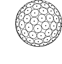
Figure 1: A possible discretization of the Bloch sphere (qubit Hilbert space). Points on each disc (of size $\epsilon$) are identified. Points between discs can be assigned to the nearest disc.

One might be concerned that the SU(2) group structure of qubit rotations cannot be obtained as the limit of larger and larger finite discrete subgroups. However, there exist simple models in which continuous rotational or even Lorentz symmetry is obtained in the long wavelength limit from underlying dynamics which has only discrete symmetry. For example, in lattice QCD the symmetries are all discrete, yet continuous symmetries emerge in the long wavelength limit. As another example, in zee a model of spinless point particles hopping on a flux lattice gives rise to low-energy excitations obeying the Dirac equation.

We can deduce similar results concerning discreteness by considering the Schrodinger equation. All the physics of a universe with discrete spacetime can be described by a wavefunction $\psi(x)$ whose values are discrete, rather than continuous. To convince ourselves of this, we need merely consider simulations of the Schrodinger equation on a classical digital computer, in which both the spacetime coordinates and $\psi(x)$ are discrete. All predictions of quantum mechanics can be obtained to any desired accuracy using such discrete simulations; quantum phenomena such as interference patterns can therefore be reproduced even if quantum mechanics is intrinsically discrete, as suggested here. Since by assumption we can probe the variation of $\psi(x)$ only over distances larger than the Planck length, the magnitude of the required accuracy $\Delta\psi$ is bounded below. (Again, since we have both ultraviolet and infrared regulators, $\psi(x)$ must be a smooth function. It cannot vanish identically in an entire region, so its variation over some finite interval is bounded below.) It is important to note, though, that the required discreteness might be exponentially small. For example, to describe the exponential tail of a wavefunction might require $\Delta\psi\sim e^{-L}$, where $L$ is the box size of the simulation. Nevertheless, for fixed $L$ and $l_{P}$, the magnitude of $\Delta\psi$ is always bounded below.

A discrete wavefunction $\psi(x)$ implies a discrete Hilbert space, and vice versa, since the value of the wavefunction is simply the overlap of a particular state, $|\psi\rangle$, with another, $|x\rangle$. In other words, using Eq. (1), $\psi(x_{i})=\langle x_{i}|\psi\rangle=a_{i}$. If the set of states $|\psi\rangle$ and the set of states $|x\rangle$ are both finite, then $\psi(x)$ can take only a finite (discrete) set of values, and vice versa. As discussed above, to accommodate exponential fall-off the size of discreteness in the $a_{i}$ must be exponentially small—potentially of order $e^{-L}$, where $L$ is the size of the universe.

However, minimal length seems to imply a stronger (non-exponential) limitation on the phase information carried by a quantum state, similar to what we obtained above for a qubit. Suppose information is stored in a particular quantum state $|\psi\rangle$. A Planck-length uncertainty in the spacetime location of the state (or of where the measurement of the state takes place) leads to an uncertainty in the value of the phase, as seen from the time translation operator $U(t)=e^{-iHt}$ or the translation operator $T(x)=e^{-ipx}$. The phase can be specified only to accuracy $E_{*}$ or $p_{*}$ in Planck units, where $E_{*}$ and $p_{*}$ are roughly the characteristic energy or momentum associated with $|\psi\rangle$. To be explicit, one can expand $|\psi\rangle$ in an energy or momentum eigenstate basis, with each term in the expansion acquiring a phase uncertainty of order $E$ or $p$. Using $p>1/L$, we obtain a phase uncertainty $\epsilon>1/L$, similar to $1/d$ in the case of a spin-$\frac{1}{2}$ qubit. If the state $|\psi\rangle$ is transported over some path in spacetime, for example to be interfered with some other state, we expect a fundamental limitation on the precision of the relative phase. This might have some interesting consequences for Berry’s phase.

We can derive this result another way by considering a particle of energy $E$, interacting with an external probe of energy $E^{\prime}$ which measures the phase $\phi$ of its wavefunction. Let the interaction take place over a time interval $\Delta t$. The phase of the particle necessarily evolves during the time interval, so $\Delta\phi\sim E\Delta t$. Causality requires $\Delta t>R$, where $R$ is the size of the probe (or the portion of it which interacts with the particle, which we take to be the entire probe). It must be the case that $R>E^{\prime}$, or the probe would have already collapsed into a black hole. Finally, using energy-time uncertainty, $E^{\prime}>(\Delta t)^{-1}$ , we obtain

$$\Delta\phi\sim E\Delta t>EE^{\prime}>E^{2}/\Delta\phi,$$ (3)

which implies $\Delta\phi>E$. So, we expect that a phase discreteness $\epsilon$ smaller than $\sim E$ (recall, we use Planck units) is undetectable experimentally.

The phase uncertainty discussed above is not inconsistent with the requirement that $\Delta\psi$ might be exponentially small. There is no contradiction between an exponentially small uncertainty in the magnitude and larger uncertainty in the phase of a wavefunction $\psi$. For example, suppose $\psi$ is expressed as the superposition of two other states: $\psi=a_{1}\psi_{1}+a_{2}\psi_{2}$. Our ability to measure $|\psi|$ (or $|\psi_{i}|$) to arbitrary accuracy places no limitation on the precision of the phases in $a_{i}$ or $\psi_{i}$.

We mention some consequences of discrete Hilbert space:

1. Only a finite number of classical bits are required to specify the state of a discrete qubit. Note that, because we cannot directly measure its state, a single qubit can be used to transmit or store only a single bit of classical information. (This is a result of Holevo’s theorem holevo .) Nevertheless, a perfect classical simulation of qubits with continuous Hilbert space requires an infinite number of classical bits.

2. There are asymptotic limits to the power of quantum computation. Consider, for example, Shor’s algorithm Shor (or similarly the quantum Fourier transform), which requires of order $(\ln n)^{3}$ steps to factor an integer $n$. Discreteness of order $\epsilon$ limits the precision of quantum manipulations, and quantum algorithms require a minimum precision of order one over the number of steps in the algorithm BBBV . Thus, factorization of an integer $n$ using Shor’s algorithm requires manipulations of precision $(\ln n)^{-3}$, and there exists a largest integer $n_{*}\sim\exp({\epsilon}^{-\frac{1}{3}})$ that can be factored. In the case of arbitrarily low-energy qubits, we might have $\epsilon\sim 1/L\sim 1/T$, where $T$ is the timescale of the quantum processor, so $n_{*}$ still grows exponentially with $T^{\frac{1}{3}}$. However, for qubits of fixed energy $E$ one eventually encounters a maximum $n_{*}$.

3. Quantum mechanics is modified at short distances. It may be that near the Planck scale the Hilbert space discreteness $\epsilon$ is of order unity. For example, a vector whose length $d$ is of order the Planck length may have only a few possible orientations (imagine that the vector must connect two points on a lattice). According to this analogy, quantum dynamics might be drastically modified at short distances. It would be interesting to formulate a superclass of models of this type which have ordinary quantum mechanics as a limiting case. These might produce a novel approach to quantum gravity, as current approaches such as string theory extrapolate quantum mechanics with continuous Hilbert space all the way to the Planck scale.

One might ask how to evolve a state in a discrete Hilbert space. There are many possibilities, but one concrete method would be to write the time evolution operator $e^{-iHt}$ as a product of discrete evolution operators $e^{-iH\Delta t}$ and apply this product of operators sequentially to the state, for example as in (2), followed by the “snap to” rule after each step. This is equivalent to taking classical digital computer simulations literally. That is, by accepting the finite precision of the variable $\psi(x)$ in an ordinary computer program, one obtains a naive discretization of Hilbert space with the “snap to” rule implemented by simple numerical rounding.

In conclusion, it appears that the traditional assumption of continuous Hilbert space is rather strong: minimal length precludes any experiment showing that the discreteness parameter $\epsilon$ is exactly zero. While we have motivated a non-zero $\epsilon$ using quantum gravity, we stress that discreteness may appear at a dimensional scale larger than $l_{P}$, and that experimentalists should keep an open mind.

Acknowledgements.— The authors thank D. Bacon, M. Graesser, B. Murray and J. Polchinski for useful comments. S. H. and R. B. are supported by the Department of Energy under DE-FG06-85ER40224. A. Z. was supported in part by the National Science Foundation under grant number PHY 99-07949(2004).

References

- (1) C. A. Mead, Phys. Rev. 135, B849 (1964); T. Padmanabhan, Class. Quant. Grav. 4, L107 (1987); For a review, see L. J. Garay, Int. J. Mod. Phys. A 10, 145 (1995).
- (2) X. Calmet, M. Graesser, S. D. H. Hsu, Phys. Rev. Lett. 93:211101, 2004, hep-th/0405033 and hep-th/0505144.
- (3) J. A. Wheeler, Ann. Phys. 2 (1957) 604; T. Regge, Nuovo Cimento A 19, 558-571, 1961; R. Penrose, Angular momentum, an approach to combinatorial space time, in Quantum Theory and Beyond, p.301, ed. T. Bastin, Cambridge University Press, Cambridge, 1971; L. Bombelli, J.H. Lee, D. Meyer, R. Sorkin, Phys. Rev. Lett. 59:521, 1987.
- (4) A. Zee, Emergence of Spinor from Flux and Lattice Hopping, in M. A. Beg Memorial Volume, (eds. A. Ali and P. Hoodbhoy), World Scientific Publishing.
- (5) A. Holevo, Bounds for the quantity of information transmitted by a quantum communication channel, Problemy Peredachi Informatsii, Vol. 9, no. 3, 1973, p. 3. English translation in Problems of Information Transmission, Vol. 9, 1973, p. 177.
- (6) P. Shor, SIAM J. Sci. Statist. Comput. 26:1484, 1997, quant-ph/9508027.
- (7) C.H. Bennett, E. Bernstein, G. Brassard, U. Vazirani, SIAM J. Sci. Statist. Comput. 26:1510, 1997, quant-ph/9701001.