String/Gauge Duality:
(re)discovering the QCD String in AdS Space

Abstract

These lectures trace the origin of string theory as a theory of hadronic interactions (predating QCD itself) to the present ideas on how the QCD string may arise in Superstring theory in a suitably deformed background metric. The contributions of ’tHooft’s large $N_{c}$ limit, Maldacena’s String/Gauge duality conjecture and lattice spectral data are emphasized to motivate and hopefully guide further efforts to define a fundamental QCD string.

Preface: Not by accident

String theory, contrary to conventional lore, was discovered not by accident but by a systematic program to build a relativistic quantum theory of the hadronic interactions without resorting to the use of local fields. The approach, referred to as “S matrix theory”, sought to impose a minimal set of consistency conditions directly on the S matrix [1]. At the time, it appeared absurd to consider the known light hadrons (pions, nucleons, etc.) as “elementary” fields, particularly with the realization that they were just the first member of a Regge family of increasingly higher masses and spins ($J\simeq\alpha^{\prime}m^{2}_{J}+\alpha_{0}$). In the language of low energy effective field theory, the difficulties in formulating a quantum field theory of hadrons and gravity were analogous. The effective low energy theory of hadrons (e.g. the pions) is the chiral Lagrangian,

$$S[U]=\int d^{4}x\{\frac{F_{\pi}^{2}}{4}\mbox{Tr}[\partial_{\mu}\Sigma^{\dagger}\partial_{\mu}\Sigma]-\frac{\langle\bar{\Psi}\Psi\rangle}{2N_{f}}\mbox{Tr}[{\cal M}\Sigma^{\dagger}+{\cal M}^{\dagger}\Sigma]+\cdots\}\;,$$ (1)

and for gravity the Einstein-Hilbert Lagrangian,

$$S[g]=\frac{M^{2}_{P}}{16\pi^{2}}\int d^{4}x\{\sqrt{-g}\;(R+\Lambda)+\cdots\}\;.$$ (2)

Both are beautiful geometric quantum theories, but they are non-renormalizable with dimensionful coupling constants inversely proportional to mass ($1/F_{\pi}$ and $1/M_{P}$). In each order of the loop expansion, one must cancel UV divergences with new higher dimensional counter terms. With the advent of QCD the analogy appeared to be lost. But it is the goal of these lectures to argue that this is not the case.

Due to dimensional transmutation QCD (with massless quarks) has a single fundamental mass scale, $\Lambda_{qcd}$, but no coupling constant. Consequent the only available “perturbative” expansion for QCD (in the infrared) is the ’tHooft expansion for small $1/N_{c}$ at fixed $\Lambda_{qcd}$. This expansion leads to a distinctly string like hadronic phenomenology. However the central question of these lectures is not the obvious existences of a phenomenological QCD string but the more basic question:

• Is the Yang Mills theory for QCD exactly equivalent (i.e. dual) to a fundamental String Theory?

This question goes beyond the existence of a confining QCD vacuum with stringy electric flux tubes to the question of a mathematically precise identity between QCD and string theory in the same sense that the Sine Gordon and Massive Thirring quantum theories are equivalent. In the latter example, not only does duality exchange strong and weak coupling expansions, but after all non-perturbative effects are included the Sine Gordon and Massive Thirring theories have identical S matrix.

For many years a similar identity between QCD and some form of string theory has been sought. At long last, recent progress in superstring theory gives this endeavor a more concrete form. Based on Maldacena’s AdS/CFT conjecture [2], backed up by almost 5 years of consistency checks, the existence of an exact Gauge/String duality between some (super) Yang Mills theories and superstrings in a non-trivial (asymptotically AdS) background is now generally accepted[3]. We now have concrete mathematical support for a generic mechanism for string/gauge duality linked to the so called “holographic principle” for any theory including quantum gravity. Naturally this has revived the search for a QCD string and brought many features into much clearer focus. These lecture will briefly review the history and recent progress in this ancient quest for the QCD string. Moreover it should be added that success in constructing a hadronic string would not only be of interest in gaining a deeper understanding of QCD but, if successful, a major step in understanding what constitutes string theory itself.

1 Lecture One: Ancient Lore

1.1 Empirical Basis

The discovery of string theory in the late 1960’s followed from a detail study of the phenomenology of hadronic scattering, specifically finite energy sum rules constrained by Regge theory at high energies. For example the Regge limit for pion elastic scattering amplitude ($\pi^{+}\pi^{-}\rightarrow\pi^{+}\pi^{-}$) was traditionally parameterized as

$$A_{\pi^{+}\pi^{-}\rightarrow\pi^{+}\pi^{-}}(s,t)\simeq g_{o}^{2}\;\Gamma[1-\alpha_{\rho}(t)]\;(-\alpha^{\prime}s)^{\alpha_{\rho}(t)}\;,$$ (3)

in Mandelstam variable $s=-(p_{1}+p_{2})^{2}$ and $t=-(p_{1}+p_{3})^{2}$. The Gamma function prefactor gives cross channel poles for rho exchange at J=1 and higher spins for $J>1$. Since the ratio for the rho width to mass is a small parameter ($\Gamma_{\rho}/m_{\rho}\simeq 0.1$), one sought a new perturbative expansions starting with a zero width approximation. This was traditionally enforced for all resonant states by using an exactly linear rho trajectory, $\alpha(t)=\alpha^{\prime}t+\alpha_{0}$, so that “resonance” poles at integer $J=\alpha(m^{2})$ had real masses [4]. In 1968 Veneziano [6] realized that exact $s,t$ crossing symmetry could be imposed by assuming an amplitude of the form,

$$A_{\pi^{+}\pi^{-}\rightarrow\pi^{+}\pi^{-}}(s,t)=g_{o}^{2}\;\frac{\Gamma[1-\alpha_{\rho}(t)]\Gamma[1-\alpha_{\rho}(s)]}{\Gamma[1-\alpha_{\rho}(s)-\alpha_{\rho}(t)]}\;,$$ (4)

the so called dual resonance model. Here “dual” referred to Dolan-Horn-Schmid duality [5] which states that the sum over s-channel resonances poles interpolates the power behavior of the leading Regge pole exchange,

$$\sum_{r}\frac{g^{2}_{r}(t)}{s-(M_{r}-i\Gamma_{r})^{2}}\simeq\beta(t)(-\alpha^{\prime}s)^{\alpha(t)}\;.$$ (5)

This property is easily derived for the dual pion scattering amplitude (4). The Regge limit follows from the Sterling’s approximation as $s\rightarrow\infty$ and the resonance expansion from the integral representation for the Beta function,

$$A_{\pi^{+}\pi^{-}\rightarrow\pi^{+}\pi^{-}}(s,t)=-g_{o}^{2}\alpha_{\rho}(t)\int^{1}_{0}dx\;x^{-\alpha_{\rho}(s)}(1-x)^{-1-\alpha_{\rho}(t)}\;.$$ (6)

Expanding at small x we get,

$$A_{\pi^{+}\pi^{-}\rightarrow\pi^{+}\pi^{-}}(s,t) = -g_{o}^{2}\sum^{\infty}_{J=1}\frac{(\alpha_{\rho}(t))(\alpha_{\rho}(t)+1)\cdots(\alpha_{\rho}(t)+J-1)}{(J-1)!}\int^{1}_{0}dx\;x^{-1-\alpha(s)+J}$$

$$\Rightarrow\sum^{\infty}_{J=1}\frac{g_{o}^{2}A_{J}(\alpha^{\prime}t)}{\alpha_{\rho}(s)-J} \simeq g_{o}^{2}\Gamma(-1-\alpha_{\rho}(t))(-\alpha^{\prime}s)^{\alpha_{\rho}(t)}\;,$$ (7)

where $A_{J}$ is a polynomial of order $J$. In fact the initial enthusiasm for this model included a striking feature of chiral symmetry. In the soft pion limit $p_{1}\rightarrow 0$, the Adler zero,

$$A_{\pi^{+}\pi^{-}\rightarrow\pi^{+}\pi^{-}}(s,t)=(1-\alpha_{\rho}(s)-\alpha_{\rho}(t))\frac{\Gamma[1-\alpha_{\rho}(t)]\Gamma[1-\alpha_{\rho}(s)]}{\Gamma[2-\alpha_{\rho}(s)-\alpha_{\rho}(t)]}\sim\alpha^{\prime}(s+t)\rightarrow 0\;,$$ (8)

is imposed if we take the phenomenologically reasonable values for the rho trajectory intercept, $\alpha_{\rho}(0)=0.5$. Further work led to the N-point generalization in Neveu and Schwarz’s seminal paper [7] entitled “Factorizable Dual Model of Pions”. So Veneziano’s amplitude turns out to be the 4-point function of the NS superstring —ignoring the conformal constraint on the Regge intercept ($\alpha(0)=1$) and the dimension of space time ($D=10$) which was not understood at the time.

As we will explain this initial enthusiasm was premature.

1.2 Covariant String Formulation

It is surprisingly easy to generalize the 4-point Beta function to get the N-point dual resonance amplitudes and the covariant quantization of the Bosonic string. The argument goes as follows. Consider the 4-point function for tachyon scattering [8] in a symmetric form,

$$\int^{1}_{0}x^{-1-\alpha(s)}(1-x)^{-1-\alpha(t)}dx=\int^{x_{3}}_{x_{1}}\frac{dx_{2}}{(x_{4}-x_{3})(x_{4}-x_{1})(x_{3}-x_{1})}\prod_{1\leq i<j\leq 4}(x_{j}-x_{i})^{2\alpha^{\prime}p_{j}p_{i}}\;,$$ (9)

where $\alpha(s)=\alpha^{\prime}s+1=2\alpha^{\prime}p_{1}p_{2}$ for $\alpha^{\prime}p^{2}_{i}=-1$. The three dummy variables maybe fixed at $x_{1}=0,x_{3}=1,x_{4}=\infty$. This does not spoil cyclic symmetry, since the integrand is invariant under Möbius transformations: $x_{i}\rightarrow(ax_{i}+b)/(cx_{i}+d)$.

Now there is an obvious guess to generalize the 4-point amplitude to N-point open string tachyon amplitude,

$$A_{N}(p_{1},\cdots,p_{N})=g_{o}^{N-2}\int\frac{dx_{2}dx_{3}\cdots dx_{N-2}}{(x_{N}-x_{N-1})(x_{N}-x_{1})(x_{N-1}-x_{1})}\prod_{1\leq i<j\leq N}(x_{j}-x_{i})^{2\alpha^{\prime}p_{j}p_{i}}\;.$$ (10)

The integration region is restricted to be $x_{1}\leq x_{2}\leq x_{3}\leq\cdots\leq x_{N}$. Modern string theory lectures or textbooks usually require hundreds of pages of derivation to write down this amplitude, if they bother to do it at all. (This is not to imply that you should not learn the formal approach to string path integral quantization but the discovery of string theory was in large part due to the simplicity of the final answer for the tree amplitude. Pedagogically it may even help to understand the answer in advance of its derivation.)

One can also follow the pioneers of the field and write down the Old Covariant Quantized string, working “backward” from the N-point function. One needs to factorize the N-point function, i.e introduce a complete set of states. Short circuiting the full derivation, this amounts to a free (string) field expansion,

$$X^{\mu}(\sigma,\tau)=\hat{q}^{\mu}-2i\alpha^{\prime}\hat{p}^{\mu}\tau+\sum^{\infty}_{n=1}\sqrt{\frac{2\alpha^{\prime}}{n}}(a^{\mu}_{n}\exp[-n\tau]+a^{\mu\dagger}_{n}\exp[n\tau])cos(n\sigma)\;$$ (11)

into normal mode oscillators,

$$[\hat{q}^{\mu},\hat{p}^{\nu}]=i\eta^{\mu\nu}\qquad\mbox{and}\qquad[a^{\mu}_{n},a^{\nu\dagger}_{m}]=\eta^{\mu\nu}\delta_{n,m}\;,$$ (12)

acting on the ground state tachyon at momentum $p$,

$$\hat{p}^{\mu}|0,p\rangle=p^{\mu}|0,p\rangle\qquad\mbox{and}\qquad a^{\mu}_{n}|0,p\rangle=0\;.$$ (13)

Then a short algebraic exercise will convince you that the integrand for the N-point function does factorize as,

$$\langle 0,p_{1}|V(x_{2},p_{2})V(x_{3},p_{3})\cdots V(x_{N-1},p_{N-1})|0,p_{N}\rangle=\prod_{1\leq i<j\leq N}(x_{j}-x_{i})^{2\alpha^{\prime}p_{j}p_{i}}$$ (14)

with

$$V(x,p) = :\exp[ipX(0,\tau)]:$$

$$= \;\exp[ip\hat{q}+ip\sum_{n}\sqrt{\frac{2\alpha^{\prime}}{n}}a^{\dagger}_{n}x^{n}]\;\exp[2\alpha^{\prime}p\hat{p}\log(x)+ip\sum_{n}\sqrt{\frac{2\alpha^{\prime}}{n}}a_{n}x^{-n}]$$

and $x\equiv\exp[\tau]$. To calculate the matrix element (i.e amplitude) one merely normal orders the operators giving factors,

$$\exp[-2\alpha^{\prime}\sum_{n}\frac{p_{i}p_{j}}{n}(\frac{x_{i}}{x_{j}})^{n}]=\exp[\alpha^{\prime}p_{i}p_{j}\log(1-x_{i}/x_{j})]=(1-\frac{x_{i}}{x_{j}})^{p_{i}p_{j}}\;,$$ (16)

for each pair of vertex insertions. The stringy interpretation follows from identification of world sheet surface co-ordinates $(\sigma,\tau)$. The above expansion for the space-time position, $X^{\mu}(\sigma,\tau)$, is a solution to the 2-d conformal equations of motion for a free string,

$$\partial_{\tau}^{2}X^{\mu}+\partial_{\sigma}^{2}X^{\mu}=0\;,$$ (17)

in Euclidean world sheet metric. Writing down the general normal mode expansion,

$$X^{\mu}(z,\bar{z})=\hat{q}^{\mu}-i\alpha^{\prime}\hat{p}^{\mu}log(z\bar{z})+\sum^{\infty}_{n=-\infty,n\neq 0}\sqrt{\frac{2\alpha^{\prime}}{|n|}}(a^{\mu}_{n}z^{-n}+b^{\dagger\mu}_{n}{\bar{z}}^{-n})\;,$$ (18)

with $z=\exp[\tau+i\sigma]$, we see that the particular solution required for the open string amplitude above satisfies Neumann boundary conditions at the ends, $\sigma=0,\pi$. The vertex function representing tachyon emission are inserted on one side at the $\sigma=0$ boundary. (Closed string have periodic boundary conditions in $\sigma$. Super strings add worldsheet 2-d fermion fields. That’s it. Sum over all worldsheet Riemann surfaces, with great care, and you have (perturbative) superstring theory.)

Nambu and Gotto took the stringy interpretation of the dual model one step further by noticing that the equation of motion (17) is a gauge fixed form for a general co-ordinate invariant world sheet (Nambu-Gotto) action,

$$S_{NG}=-\frac{1}{2\pi\alpha^{\prime}}\int d^{2}\xi\sqrt{-det(h)}\;,\qquad\mbox{where}\qquad h_{\alpha\beta}=\partial_{\alpha}X^{\mu}\partial_{\beta}X_{\mu}\;,$$ (19)

with surface tension $T_{0}=1/(2\pi\alpha^{\prime})$. At the classical level this is also equivalent to the Polyakov form,

$$S_{P}=-\frac{1}{2\pi\alpha^{\prime}}\int d^{2}\xi\sqrt{-det(\gamma)}[\gamma^{\alpha\beta}\partial_{\alpha}X^{\mu}\partial_{\beta}X_{\mu}]\;,$$ (20)

with an auxiliary “Lagrange multiplier” 2-d metric, $\gamma_{ij}$. However the Polyakov form is easier to gauge fix and quantize using BRST technology [8]. To get a feeling for the dynamics of the open string, it is interesting to write down a few classical solutions [9].

1.3 Two Open String Solutions

One can write down the Euler Lagrange equations for the Nambu-Gotto string action and use diffeomorphism invariance, $\tau^{\prime}=f(\sigma,\tau),\sigma^{\prime}=g(\sigma,\tau)$, to choose a gauge. The static ($t=X^{0}=i\tau$) orthogonal ($h_{12}=h_{11}+h_{22}=0$) gauge is a useful choice. This gives a linearize equation of motion

$$\partial_{t}^{2}X^{\mu}-\partial_{\sigma}^{2}X^{\mu}=0\;,$$ (21)

with constraints,

$$\partial_{\sigma}X^{\mu}\partial_{t}X_{\mu}=0\qquad\partial_{t}X^{k}\partial_{t}X_{k}+\partial_{\sigma}X^{k}\partial_{\sigma}X_{k}=1\;.$$ (22)

Solution # 1: The string stretch along the 3rd axis with (fixed) Dirichlet boundary conditions, $\sigma\in[0,L]$: All spatial components $X^{k}=0$ except,

$$X^{3}=\sigma\;,$$ (23)

with energy $E_{0}=T_{0}L$ exhibiting linear confinement. For future reference the exact quantum solution has energy,

$$E_{n}=T_{0}L\sqrt{1-\frac{\pi(D-2)}{12T_{0}L^{2}}+\frac{2\pi a^{\dagger}_{n}a_{n}}{T_{0}L^{2}}}$$ (24)

for D space-time dimensions.

Solution # 2: The free string rotating in the $(X_{1},X_{2})$ plane with Neumann boundary conditions, $\sigma\in[0,\pi L/2]$: All spacial components $X^{k}=0$ except,

$$X^{1}+iX^{2}=(L/2)\cos(2\sigma/L)\exp[i2t/L]\;,$$ (25)

with energy $E=\pi LT_{0}/2$ and total angular moment (spin) $J=\alpha^{\prime}E^{2}$. This last result ($J\sim E^{2}$), which is the key requirement for QCD Regge phenomenology, is a rather non-trivial property of a relativistic massless string. The end points always travel at the speed of light, so as the energy increases the string gets longer BUT the angular velocity decreases: $\omega=2/L=1/(\pi T_{0}E)$. Nonetheless the angular momentum increases quadratically because at constant tension the total stored energy grows linearly in L and the moment of inertia grows as a cubic, $L^{3}$. This is in stark contrast with a rigid non-relativist bar where $J\sim E^{1/2}$. Clearly the linear Regge trajectory support the general picture of a massless “flux” tube with energy coming entirely from its tension. Again for future reference the exact quantum state for this leading trajectory is

$$(a^{1}_{(1)}+ia^{2}_{(1)})^{J}|0,p\rangle\;.$$ (26)

1.4 Failure of the Old QCD String

We should now take a break from this discourse and learn all of rules of superstring perturbations theory [10]. With the help of anomaly cancellation, we would discover 5 consistent perturbation expansions — free of tachyons and negative norm (i.e. ghost) states. The resulting phenomenology for perturbative superstrings (in flat space-time) has 4 disasters from the view point of a QCD string:

1. Zero mass states (i.e $1^{-}$ gauge/ $2^{++}$ graviton)

2. Supersymmetry

3. Extra dimension: $4+6=10$

4. No Hard Scattering Processes

One can easily imagine that the first 3 difficulties could be remedied by “forcing” some form of compactification of the extra 6 dimensions, breaking all unwanted symmetries. Indeed in view of the fact that superstrings include gravity, it is even natural to suppose that solutions should include non-trivial space-time geometries. However the 4th problem (no hard scattering) reveals a fundamental mismatch between soft strings and hard partonic QCD. All in all an abject failure for QCD strings – albeit a very interesting framework for a theory of quantum gravity interacting with matter. A theory of Everything perhaps. There are two possible consequence, either the fundamental QCD string has nothing to do with a fundamental superstring or there are dramatic new effects when non-trivial background metrics are considered.

2 Lecture Two: Gauge/String Duality

In a sense the modern era of the QCD string begins almost immediately after the discovery of QCD itself with ’tHooft analysis [11] of the large $N_{c}$ limit in 1974. The problem he faced was to understand how the picture of valence quarks attached to the strings of the dual resonance model might arise in QCD. Even assuming some non-perturbative mechanism for electric confinement, one must find a small parameter to explain the zero resonance width approximation.

2.1 Large $N_{c}$ Topology

Note that full quantum theory for QCD has in fact no coupling constant because by dimensional transmutation (or breaking of conformal symmetry at zero mass for the quarks) this coupling is replaced by a fundamental mass scale, $\Lambda_{qcd}$. Thus SU(3) Yang Mills theory has in fact no free dimensionless parameters relative to the intrinsics QCD scale $\Lambda_{qcd}$, except for the masses of the quarks $m_{q}/\Lambda_{qcd}$ and the $\theta$ parameter. The so called weak coupling expansion for QCD, is a shorthand for the loop expansion in $\hbar$ which is of course of great use in the UV for large “energies”, $E/\Lambda_{qcd}$, due to “asymptotic freedom”.

Consequently, ’tHooft asked whether the inverse of the rank of the group for $SU(N_{c})$ Yang-Mills theory could be used as a formal expansion parameter. Term by term in the loop expansion in $\hbar$, he suggested expanding in $1/N_{c}$ holding fixed the ’tHooft coupling $g^{2}_{YM}N_{c}$. Resumming each contribution to $(1/N_{c})^{n}$, the result is the famous topological restructuring of the loop expansion as sum over Riemann surfaces. The derivation proceeds as follows. Starting from the action,

$$S=\frac{1}{g^{2}_{YM}}Tr[(\partial_{\mu}A_{\nu}-\partial_{\nu}A_{\mu}+i[A_{\mu},A_{\nu}])^{2}]+\frac{1}{g^{2}_{YM}}\bar{\Psi}(\gamma_{\mu}\partial_{\mu}-iA_{\mu})\Psi\;,$$ (27)

we write down Feynman expansion tracing the color and flavor flow in the “double line” diagramatics and count factors of $1/N_{c}$:

Gluon Loops $$: \delta^{r}_{r}=N_{c}\;\Rightarrow O(N_{c}^{F})$$

Gluon & Quark Prop $$: g^{2}_{YM}=g^{2}_{YM}N_{c}\times\frac{1}{N_{c}}\;\Rightarrow\;O(N_{c}^{-E})\;,$$

Vertices $$: \frac{1}{g^{2}_{YM}}=\frac{1}{g^{2}_{YM}N_{c}}\times N_{c}\Rightarrow\;O(N_{c}^{V})\;.$$ (28)

Using Euler’s theorem the factors of $N_{c}$ for color loops (faces F), gluon/quark propagators (edges E), interactions (vertices V) is rewritten and quark flavor loops (boundaries B),

$$N_{c}^{F-E+V-B}=N_{c}^{\chi}=N_{c}^{2-2H-B}\;,$$ (29)

depending only on the topology of the graph as function of the number of glueballs propagators (i.e. handles H) and the quark loops ( i.e.boundaries B). This is precisely the topological expansion of string theory in terms of the genus of the world sheet.

Perhaps more significant this topology can also be shown to hold on the lattice in the strong coupling confining phase. On the lattice the strong coupling expansion is actually a sum over surfaces of electric flux so in spite of the extreme breaking of Lorenz invariance due the lattice, the physical mechanism for confinement is clearly string-like flux tubes. The derivation is analogous to weak coupling. For illustration consider the Wilson form of the pure gauge action,

$$S=\frac{1}{g^{2}_{YM}}\sum_{P}Tr[2-U_{P}-U^{\dagger}_{P}]\quad,\quad U_{P}=U_{\mu}(x)U_{\nu}(x+\mu)U^{\dagger}_{\mu}(x+\nu)U^{\dagger}_{\nu}(x)\quad,\quad U_{\mu}=\exp[iaA_{\mu}]\;.$$

as a sum over plaquettes. In strong coupling the action is expanded in a power series and each link variable ($U_{\mu}(x)$) is integrated over its Haar measure. To get a non-zero result every link in the expansion must be paired with (at least) one anti-link ($U\rightarrow U^{\dagger}$). This leads immediately to the rule:

Plaquettes $$: \frac{1}{g^{2}_{YM}}=\frac{1}{g^{2}_{YM}N_{c}}\times N_{c}\;\Rightarrow O(N_{c}^{F})\;,$$

Links $$: \int dU\;U^{l_{1}}_{r_{1}}U^{\dagger r_{2}}_{l_{2}}=\frac{1}{N_{c}}\delta^{l_{1}}_{l_{2}}\delta^{r_{2}}_{r_{1}}\;\Rightarrow\;O(N_{c}^{-E})\;,$$

Sites $$: \delta^{r}_{r}=N_{c}\;\Rightarrow\;O(N_{c}^{V})\;,$$ (30)

Treating quark loops boundaries as before, Euler’s theorem yields exactly the same topological result as in weak coupling (ignoring self-intersections of surfaces). However it should be realized that the meaning is quite different. The vertices give the index sums, the faces are now field strengths and edges are not propagators. Apparently the topology of large $N_{c}$ Yang Mills is a robust feature in need of a deeper explanation.

In a real sense the large $N_{c}$ limit if it exists can be considered as one possible definition of the QCD string perturbative expansion order by order in the string coupling $g_{s}\sim 1/N_{c}$. But to go beyond this theoretical assertion by explicitly take the large $N_{c}$ limit to give a mathematical tractable formulation of the perturbative QCD string (even for the leading term at $N_{c}=\infty$) has proven frustrating, except for two dimensional QCD. Also it is interesting to note that there is more than one large $N_{c}$ limit [12]. One can choose to treat quark field as an anti-symmetric tensor, $\Psi^{ij}=\epsilon^{ijk}\psi_{k}$ in color. If one now takes the large $N_{c}$ limit of 1 flavor QCD with this tensor representation for quark fields, the fermion loop is no longer subdominant. Now the leading term can be shown to be precisely the same as the large $N_{c}$ limit of ${\cal N}=1$ SUSY Yang Mills theory! Should we be alarmed at this in view of the glib statement that the large $N_{c}$ limit defines string perturbation theory. I think not. In fact the full non-perturbative QCD string theory might well have more than one weak coupling string expansion, analogous to the now conventional view of superstrings in 10-d.

2.2 AdS/CFT correspondence for Superstrings

String theory has undergone a tremendous transformation in the last 35 years. In the “First String Revolution” perturbative string vacua were restricted to five alternatives (IIA, IIB, I, H0, HE) by the requirement to cancel tachyons, ghosts and anomalies. This appeared to restrict dramatically the space of possible string theory. In the “Second String Revolution”, non-perturbative dualities even related these 5 cases (and M theory) into a single connected manifold. However, that is not the end of the story. Solitonic objects called D-brane have given rise to a tremendous explosion of possible vacua so in the infrared the physics of strings in non-trivial backgrounds are seen to mimic a plethora of effective fields theories.

In 1998 Maldacena [2] realized that at least under certain circumstances string theories had to be dual (i.e. equivalent) to Yang Mills theory. While this is technically still a conjecture, consistency relations are now so extensive that the existence of exact String/Gauge dualities in many special circumstances is hard to doubt.

The first example was IIB superstrings (or in the low energy limit IIB supergravity) propagating in an $AdS^{5}\times S^{5}$ 10-d manifold,

$$ds^{2}=\frac{r^{2}}{R^{2}}\sum^{3}_{\mu=0}\eta_{\mu\nu}dx^{\mu}dx^{\nu}+\frac{R^{2}}{r^{2}}\;(dr^{2}+r^{2}d^{2}\Omega_{5})$$ (31)

which is dual to 4-d $\cal N$ = 4 Super SU($N_{c}$) Yang Mills theory. The $(x_{\mu},r)$ co-ordinates form the $AdS^{5}$ manifold with negative curvature with radius $R$ fibered by a $S^{5}$ sphere of (positive) radius R and metric $d^{2}\Omega_{5}$. The motivation for this duality is based on the background metric for a set of $N_{c}$ parallel massive D3 sources (see Fig. 1). Evidence had accumulated that there are two equivalent ways to model the dynamics of D3 branes. First by considering short open strings attached to the branes which at low energies is SUSY Yang Mills (SYM) theory and second by the near horizon fluctuations of closed IIB superstrings or at low energy IIB supergravity. The leap of faith was to conjecture that in the near horizon limit these are exactly equivalent. In a sense this is the old open/closed string duality in a different context.

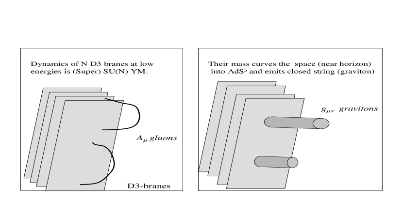
Figure 1: Open/closed string duality for $N_{c}$ D3 branes leading to the conjecture duality of IIB strings in $AdS^{5}\times S^{5}$ and $\cal N$ = 4 Super SU($N_{c}$) Yang Mills theory.

In this dual correspondence, the string (or gravity) correlation functions as you approach the boundary of $AdS^{5}$ ($r\rightarrow\infty$) are equivalent to the gauge invariant correlators in SYM theory. The discrete “Kaluza-Klein” modes in $S^{5}$ give the multiplets under SYM R symmetry $SU(5)$. By combining the subtle new idea of holography in r and the more mundane Kaluza-Klein mechanism on $S^{5}$, we see how a 10-d string can be dual to a 4-d field theory. There is no loss of degrees of freedom. The ’tHooft gauge coupling is $g^{2}_{YM}N_{c}=R^{4}/\alpha^{\prime 2}$ where the intrinsic string length scale is $\sqrt{\alpha^{\prime}}=l_{s}$. Consequently ’tHooft’s strong coupling gauge theory is dual to weak coupling gravity ($l_{s}\sim l_{Planck}$) and the $1/N_{c}$ expansion parameter is identified with the closed string coupling constant $g_{s}=g^{2}_{YM}\sim 1/N_{c}$ as one would expect from the large $N_{c}$ topological expansion.

Although the Maldacena string/gauge duality is believed to hold for general coupling and general $N_{c}$, it is difficult to quantize even free strings ($N_{c}=\infty$) in this background which includes a non-zero Ramond-Ramond flux. In the strong coupling limit ($g_{s}\sim g^{2}_{YM}\rightarrow\infty$), the string tension diverges leaving only the center of mass motion of closed strings, which is equivalent to IIB gravity in the tree approximation. The weak coupling limit of classical gravity is easily solved. (Other special cases, such as the pp-wave limit, are tractable as well.)

2.3 Confinement

One may view the correspondence in holographic terms. The Yang Mills UV (short distance) degrees of freedom are dual to excitations near to the AdS boundary at $r\rightarrow\infty$, while the IR (long distance physics) is represented by modes at small $r\rightarrow 0$. This mapping is referred to as IR/UV correspondence. A graphic illustration of this IR/UV correspondence is afforded by the scale breaking instanton solution to Yang-Mills located at $x^{\mu}$ with size $\rho$. This corresponds exactly to 0-brane located at five dimensional co-ordinate $(x^{\mu},r=1/\rho)$ in the $AdS^{5}$ manifold.

Ironically this first example of Yang-Mills/String duality does not confine because the quantum field theory is exactly conformal. Wilson loops have pure Coulomb (rather than area law) behavior. When a large Wilson test loop is introduced on the boundary of AdS, the red shift factor $r^{2}/R^{2}$ of the metric allows the minimal surface area spanning the loop to remain finite by moving into the interior nearer and nearer to $r=0$.

To look for models closer to QCD we must break conformal and supersymmetries. These models typically modify the metric in the IR cutting it off at a finite value $r=r_{min}$. Two simple examples were suggested by Witten by introducing a Euclidean AdS black hole background with a compact dimension (called $\tau$) whose radius set by the Hawking temperature:

• $AdS^{5}\times S^{5}$ Black Hole for 10-d IIB string theory

• $AdS^{7}\times S^{4}$ Black Hole for 10-d IIA string theory

Both metrics have the general form,

$$ds^{2}=\frac{r^{2}}{R^{2}}\eta_{\mu\nu}dx^{\mu}dx^{\nu}+\frac{R^{2}}{r^{2}[1-(r_{min}/r)^{d}]}\;dr^{2}+\frac{r^{2}}{R^{2}}[1-(r_{min}/r)^{d}]\;d\tau^{2}+ds^{2}_{X}\;.$$ (32)

The horizon of the black hole introduces a scale breaking cut-off, which we can identify roughly with $\Lambda_{qcd}=1/r_{min}$ or as we will see subsequently the scale of the glueball mass in strong coupling.

In these black hole metrics, the minimal area surface spanning a Wilson loop of increasing size eventually must approaches $r=r_{min}$. At this point the area of the surface no longer has a red shift factor and it grows proportional the physical area of the Wilson loop itself. For example in the $AdS^{5}$ black hole the proper areas grows proportional to $r^{2}_{min}R^{2}$ giving a QCD tension $T_{qcd}=1/2\pi\alpha^{\prime}_{qcd}$ or Regge slope,

$$\alpha^{\prime}_{qcd}=\alpha^{\prime}/R^{2}r^{2}_{min}=\Lambda^{2}_{qcd}/\sqrt{2g^{2}_{YM}N_{c}}$$ (33)

2.4 Hard Scattering at Wide Angles

We know that QCD, even in leading order of large $N_{c}$, exhibit asymptotic freedom and hard parton scattering properties. Consequently for the QCD string, one of the most baffling features in flat space is the complete absence of hard scattering. One the other hand for the application of string theory to quantum gravity, this softening of the short distance physics is a virtue, which is responsible for a finite weak coupling limit. Here we explain a surprisingly simple mechanism to reconcile this apparent conflict for strings duals to Yang-Mills theory.

Let us begin with a description of the fundamental “Rutherford experiment” for hadrons – scattering two hadrons at wide angles. It is known that QCD exhibits power law fall off at wide angles precisely due to hard (UV) processes

$$A_{qcd}(s,t)\sim(\frac{1}{\sqrt{\alpha^{\prime}_{qcd}s}})^{n-4}\;,$$ (34)

where $n=\sum_{i}n_{i}=\sum_{i}(d_{i}-s_{i})$ is give as the sum over the twist ($n_{i}$) for each external state. In stark contrast the fundamental strings (in flat space) exhibits exponentially damped wide angle scattering,

$$A_{closed}(s,t)\rightarrow\exp\big{[}-\frac{1}{2}\alpha^{\prime}(s\ln s+t\ln t+u\ln u)\big{]}\;.$$ (35)

Polchinski and Strassler [13] made the essential observation on how string scattering in a confining background AdS background might avoid this conflict with QCD. Suppose you have a background that is cut-off for small $r<r_{min}$ and approximated by $AdS^{5}\times X_{5}$ for large r,

$$ds^{2}=\frac{r^{2}}{R^{2}}\eta_{\mu\nu}dx^{\mu}dx^{\nu}+\frac{R^{2}}{r^{2}}dr^{2}+ds^{2}_{X}\;.$$ (36)

A plane wave external glueball ($\phi(r)\exp[ixp]$) at strong coupling scatters locally in r through a string amplitude with a red shifted proper distance or equivalently an effective momenta,

$$\hat{p}_{s}(r)=\frac{R}{r}p\;.$$

Relative to the string scale, $l_{s}=\sqrt{\alpha^{\prime}}$, the exponential cut-off at high momenta ($l_{s}p_{s}>1$), suppresses string scattering in the IR region ($r<r_{scatt}$), leaving a residual amplitude in a decreasingly small window in the UV ($l_{s}p_{s}<1$),

$$r>r_{scat}\equiv\sqrt{\alpha^{\prime}}Rp\;.$$

Since the tail of the glueball wavefunction, $\phi_{i}(r)\sim(r/r_{min})^{-\Delta^{(i)}_{4}}$, is entirely determined in the String/Gauge dictionary by the conformal weight $\Delta^{(i)}_{4}$ of the corresponding gauge operator dual to the string state, one is led back to the standard parton or naive dimensional analysis result used in the wide angle power counting,

$$\phi_{i}(r_{scat})\sim\Big{(}\frac{r_{scat}}{r_{min}}\Big{)}^{-\Delta^{(i)}_{4}}\sim(\sqrt{\alpha^{\prime}_{qcd}}\;p)^{-\Delta^{(i)}_{4}}\;,$$ (37)

where we have converted to the hadronic scale, $\alpha^{\prime}_{qcd}\sim(R/r_{min})^{2}\alpha^{\prime}$ .

In the corresponding M-theory construction (sometime referred to as M-QCD), all of this appears to be upset because the scaling of the wave function in $AdS^{7}$ changes. For example the scalar glueball with interpolating field $Tr[F^{\mu\nu}F_{\mu\nu}]$ in $AdS^{5}$ has $\Delta_{4}=4$ as expected but in $AdS^{7}$ the wavefunction scales with $\Delta_{6}=6$ at large r. As pointed out by Brower and Tan [14], this apparent conflict with partonic expectations is avoided when one realizes that from an M-theory perspective, strings are a consequence of membranes wrapping the “11th” dimension and that in $AdS^{7}$ this 11th dimension is warped just like another spatial coordinate ($x^{\mu}$) with the proper size: $\hat{R}_{11}(r)=(r/R)R_{11}$. To account for this effect, one can introduce local values for the effective string length and coupling constant,

$$\hat{l}^{2}_{s}(r)=\frac{R}{r}(l^{3}_{p}/R_{11})\;,\quad{and}\quad\hat{g}^{2}_{s}(r)=\frac{r^{3}}{R^{3}}(R^{3}_{11}/l^{3}_{p})\;.$$

as a function of the local scattering position in r. This additional deformation is precisely what is required. The new definition of the scattering region at wide angles,

$$r>r_{scat}=\hat{l}_{s}(r_{scat})R\;p=\sqrt{\alpha^{\prime}}\;R^{\frac{2}{3}}\;r_{scat}^{-\frac{1}{2}}\;p\;,$$

leads to

$$\phi_{i}(r_{scat})\sim\Big{(}\frac{r_{scat}}{r_{min}}\Big{)}^{-\Delta^{(i)}_{6}}\sim\Big{(}\sqrt{\alpha^{\prime}_{qcd}}\;p\Big{)}^{-\frac{2}{3}\Delta^{(i)}_{6}}$$ (38)

for each external line. For example, for the $0^{++}$ scalar glueball corresponding to interpolating YM operator $Tr[F^{2}]$, the factor of $2/3$ exactly compensates for the the shift in the conformal dimension from $\Delta_{4}=4$ for $AdS^{5}$ to $\Delta_{6}=6$ for $AdS^{7}$ to give the parton results, $n_{i}=\frac{2}{3}\Delta^{(i)}_{6}$. This time, in converting to the hadronic scale in Eq. 38, we must realize the relationship of $\alpha^{\prime}_{qcd}$ to the string scale is

$$\alpha^{\prime}_{qcd}\sim(R/r_{min})^{3}\alpha^{\prime}\;,$$ (39)

which differs from the $AdS^{5}$ string relation (33). The 3rd power is a consequence of the fact that in M-theory the area law for the Wilson loop really comes from a minimal volume for a wrapped membrane world volume stabilized at $r\simeq r_{min}$ rather than a minimal world surface area for a string which gave quadratic behavior in Eq. 33 .

Putting all factors together, the result for M-theory can be expressed as,

$$\Delta\sigma_{2\rightarrow m}\simeq\frac{1}{s}\;f(\frac{p_{i}\cdot p_{j}}{s})\frac{1}{N^{2m}}\;\prod_{i}\Big{(}\frac{1}{\alpha^{\prime}_{qcd}s}\Big{)}^{n_{i}-1}\;,$$

in correspondence with the weak-coupling QCD result.

Summarizing the results on hard scattering:

1. $AdS^{5}$ by Polchinski-Strassler: $\Delta\sigma_{2\rightarrow m}\simeq\frac{1}{s}\;f(\frac{p_{i}\cdot p_{j}}{s})\frac{(\sqrt{g^{2}N_{c}})^{m}}{N_{c}^{2m}}\;\prod_{i}\Big{(}\frac{1}{\alpha^{\prime}_{qcd}s}\Big{)}^{n_{i}-1}$

2. $AdS^{7}$ by Brower-Tan: $\Delta\sigma_{2\rightarrow m}\simeq\frac{1}{s}\;f(\frac{p_{i}\cdot p_{j}}{s})\frac{1}{N_{c}^{2m}}\;\prod_{i}\Big{(}\frac{1}{\alpha^{\prime}_{qcd}s}\Big{)}^{n_{i}-1}$

3. QCD perturbation theory: $\Delta\sigma_{2\rightarrow m}\simeq\frac{1}{s}\;f(\frac{p_{i}\cdot p_{j}}{s})\frac{(g^{2}N_{c})^{m}}{N_{c}^{2m}}\;\prod_{i}\Big{(}\frac{g^{2}N\Lambda_{qcd}^{2}}{\alpha^{\prime}_{qcd}s}\Big{)}^{n_{i}-1}$

2.5 Near-Forward Scattering and Regge Behavior

The importance of scattering at large r also implies the presence of a hard component in the near-Regge limit, $t/s\rightarrow 0$ as $s\rightarrow\infty$. The approximation of a single local scattering leads to $T(s,t)=\int_{r_{h}}^{\infty}dr\;{\cal K}(r)A(s,t,r),$ where $A$ is a local 4-point amplitude, ${\cal K}(r)\sim r^{5}\phi_{1}(r)\phi_{2}(r)\phi_{3}(r)\phi_{4}(r)$, up to a constant, and $r_{h}$ is a cut-off, $r_{h}>>r_{min}$. After converting to local string parameters as discussed above, the amplitude $A(s,t,r)$ depends only on $\alpha^{\prime}\hat{s}$ and $\alpha^{\prime}\hat{t}$, where $\hat{s}=(R/r)^{3}s$ and $\hat{t}=(R/r)^{3}t$. In the Regge limit the amplitude becomes

$$T(s,t)=\int_{r_{h}}^{\infty}dr\;{\cal K}(r)\beta(\hat{t})(\alpha^{\prime}\hat{s})^{\alpha_{0}+{\alpha^{\prime}}\hat{t}}\;.$$ (40)

For small $t\simeq 0$, this corresponds to an exchange of a BFKL-like Pomeron, with a small effective Regge slope,

$$\alpha^{\prime}_{BFKL}(0)\sim(r_{min}/r_{h})^{3}\alpha^{\prime}_{qcd}<<\alpha^{\prime}_{qcd}\;.$$ (41)

Such an exchange naturally leads to an elastic diffraction peak with little shrinkage. In the coordinate space, one finds, for a hard process, the transverse size is given by

$$\langle{\vec{X}}^{2}\rangle\sim(r_{min}/r_{h})^{3}\alpha^{\prime}_{qcd}\log s+{\rm constant}\;.$$ (42)

If the cutoff, $r_{h}$, which characterizes a hard process, increases mildly with $s$, e.g. $r_{h}^{3}\sim\log s$, there will be no transverse spread. In the language of a recent study by Polchinski and Susskind, [15], this corresponds to “thin” string fluctuation.

In spite of this progress in seeing some partonic effects in the string picture, there is much more to understand. For instance, we note that, consistent with the known spectrum of glueballs at strong coupling, the IR-region must in addition give a factorizable Regge pole contribution,

$$T(s,t)\sim A(s,t,r_{min})\sim(\alpha^{\prime}_{qcd}s)^{\alpha_{P}(0)+\alpha^{\prime}_{qcd}t}\;.$$ (43)

In our M-theory construct [16], $\alpha_{P}(0)=2-0(1/g^{2}N)$. Of course, this “soft” Pomeron must mix with the corresponding hard component, leading to a single Pomeron singularity in the large N limit. However, addressing this issue requires a more refined treatment for the partonic structure within a hadron. As emphasized by Polchinski and Strassler in a recent paper [17], this is also what is required for treating deep inelastic scattering in the string/gauge duality picture. Efforts in this direction are currently underway.

3 Lecture Three: String vs Lattice Spectra

Based on the conformally broken backgrounds using Maldacena string/gauge duality, we can begin to do some calculation in QCD like theories, at least in the strong coupling limit. This is still far from the hoped for discovery of the QCD string. We are in the position somewhat similar to a lattice cut-off theory. The strong coupling limit brings along non-universal cut-off dependent effects. However unlike the lattice, we have (as yet) no algorithm (theoretical or numerical) to in principle send the cut-off to infinity. String/gauge duality presents a coupled problem, even in the large $N_{c}$. The world sheet sigma model for the string theory emits gravitons that perturb the background which in turn has a back reaction on the sigma model. Even finding the sigma model beta function perturbatively to the next order in $1/\alpha^{\prime}$ is difficult. Still it is worth while to see if there is a reasonable spectrum in strong coupling approximation.

On the lattice side, where one can numerically take the weak coupling (continuum) limit, the spectra for glueballs and the quantum states of a stretch string are becoming quiet accurately determined. Even extrapolating this spectra to the large $N_{c}$ limit has met with some success. In short the lattice has given and is capable of giving more accurate spectral data for the quantum QCD string. If it exists, there can be only one answer. This is a unique opportunity: A concrete string theory problem with copious “experimental” data to constrain its construction!

3.1 Glueball Spectra

The first such lattice AdS/CFT comparison was the computation of the strong coupling glueball spectrum in the $AdS^{7}$ M-theory black hole. The correspondence for the quantum numbers for the gravity modes in terms of the Yang-Mill fields are read off the effective Born-Infeld action on the brane,

$$S=\int d^{5}x\det[G_{\mu\nu}+e^{-\phi/2}(B_{\mu\nu}+F_{\mu\nu})]+\int d^{4}x(C_{1}F\wedge F+C_{3}\wedge F+C_{5})$$ (44)

The entire spectrum for all states in the QCD super selection sector are now known and can be compared with lattice data for SU(3). The comparison is rather encouraging considered as a first approximation (see Fig. 2). All the states are in the correct relative order and the missing states at higher J are a direct consequence of strong coupling which pushes the string tension to infinity.

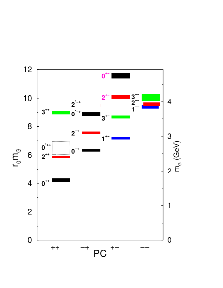
Figure 2: The AdS glueball spectrum [16] for $QCD_{4}$ in strong coupling (left) compared with the lattice spectrum [18] for pure SU(3) QCD (right). The AdS cut-off scale is adjusted to set the lowest $2^{++}$ tensor state to the lattice results in units of the hadronic scale $1/r_{0}=410$ Mev.

It appears plausible that the $AdS^{7}$ black hole phase at strong coupling is rather smoothly connected to the weak coupling (confined) fixed point of QCD. However it must be stated that there is no general understanding of how the metric will be deformed so that all the unwanted charged Kaluza-Klein states in the extra compact directions decouple. All attempts to find better background solutions to supergravity as a starting point for QCD have failed in this regard.

3.2 Stretched String Spectra

An even more direct observation of the string spectrum in lattice gauge data is giving by the quantum modes of a stretch string between fixed infinitely heavy sources (see Fig 3). This is the open QCD string with Dirichlet boundary conditions. From the $AdS/CFT$ view point starting with the string ends separated by a small distance L, we are able to see first the short distance coulomb regime. Then as we increase L, the minimal surface moves into the interior probing more and more IR physics. Finally at very large L, we see only the $O(1/L)$ low mass pseudo Goldstone modes for the transverse co-ordinates of the string leading to the universal spectrum of Lüscher,

$$E=T_{0}L-\frac{\pi(D-2)}{12L}+\frac{2\pi a^{\dagger}_{n}a_{n}}{L}+\cdots$$ (45)

Indeed at large separation L the lattice data for the stretched string spectrum appears to be approaching this form with $D-2=2$ transverse oscillators (See fig 3).

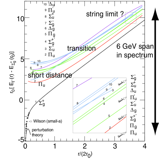
Figure 3: Quantum fluctuation of a stretch QCD flux tube [19]

Very careful and clever methods have been develop by Lüscher and Weisz [20] to determine the universal “Lüscher term” giving a fit in the range 0.5 to 1.0fm to the ground state (i.e. static potential):

$$E_{0}(L)=\frac{\pi}{12}(1+0.12fm/L)$$

confirming this prediction.

A major challenge to the AdS/CFT approach to the QCD string is to understand the interpolation between large L and small L. If we take as a model, the “warped” metric,

$$ds^{2}=V(y)dx^{\mu}dx_{\mu}+dy^{2}+U(y)d^{2}\tau+\cdots$$ (46)

suggested by an $AdS^{d+2}$ black hole with $V(y)=r^{2}/r^{2}_{min}=[cosh(\frac{d+1}{2}ky)]^{4/(d+1)}$. We can solve (numerically) for the classical minimal surface getting a potential energy, $E_{0}(L)$, for the classical ground state stretched string. For $d=3$ and $R^{4}=2g^{2}_{YM}N_{c}\alpha^{\prime 2}$, it has the limiting values,

$$E_{0}\rightarrow\frac{r^{2}_{min}}{2\pi R^{2}\alpha^{\prime}}\;L+O(Le^{-cL})\qquad\mbox{and}\qquad E_{0}\rightarrow-\frac{(2\pi)^{2}}{\Gamma(1/4)^{4}}\;\frac{\sqrt{2g^{2}_{YM}N_{c}}}{L}$$ (47)

for $L\rightarrow\infty$ and $L\rightarrow 0$ respectively. The shape of the potential,$E_{0}(L)$, fits the lattice data almost perfectly after setting the QCD length scale ($r_{min}=/\Lambda_{qcd}$) and string tension ($T_{qcd}=1/2\pi\alpha^{\prime}_{qcd}=r^{2}_{min}/2\pi R^{2}\alpha^{\prime}$). This is reassuring but also highlights the present situation. QCD itself in the continuum limit will give a definite number for the string tension, $T_{qcd}$ (at large N) relative to the QCD scale, $\Lambda_{qcd}$. But at strong coupling in the AdS/CFT (or on the strong coupling lattice for that matter), there is an extra parameter that allows these to fixed independently. One must flow to the asymptotically free UV fixed point to eliminate this parameter.

Work is currently underway to study the fluctuations as well in this model background [21]. In a gauge with $\sigma=z=X^{3}$ the transverse fluctuation obey the equation,

$$[\;\partial^{2}_{t}-v^{2}(z)\partial^{2}_{\sigma}\;]\;X_{\perp}=0\;,$$ (48)

and the radial mode,

$$[\;\partial^{2}_{t}-v^{2}(z)\partial^{2}_{\sigma}\;]\;\xi=M^{2}(z)\xi\;,$$ (49)

with $v^{2}(z)=V^{2}(0)/V^{2}(z)$ and $M^{2}(z)=V^{2}(0)[\;V^{\prime\prime}(z)/V^{2}(z)-3V^{\prime 2}(z)/2V^{3}(z)\;]\simeq constM^{2}_{BG}$ choosing the string to stretch symmetrically in the interval $z\in[-L/2,L/2]$. The local velocity of waves on the string $v(z)$ is bounded by the speed of light, slowing as it approaches the infinitely massive quarks at the ends. It is clear that at large L this will reproduce the Lüscher result for a D-2 = 2 string. In addition there are quantum modes for fluctuations in the extra “radial” directions with a rest mass set by the glueballs. These modes correspond through string/gauge duality to longitudinal modes for a fat chromodynamic flux tube. However this toy QCD string is at best just a qualitative model of how a QCD string in warped space might behave. To find the microscopic degrees of freedom on the world sheet for the QCD string will require a detailed understanding of how high frequencies are governed by the short distance properties of asymptotically free gauge theory at large $N_{c}$.

4 No Conclusions Yet

The construction of the QCD string theory remains a tantalizing but unrealized goal. Recent progress has certainly begun to show how such an exact string/gauge duality may arise. Indeed the intimate relations between Yang-Mills theory and string theory is a dramatic change in our understanding, which may aptly designated the “First String Counter Revolution” – bring the subject back to its earliest roots. In these short lecture notes it has not been possible to describe fascinating new insight into issues concerning the introduction of dynamical quarks, spontaneous chiral symmetry breaking, non-perturbative effects in the coupling $g_{s}\sim 1/N_{c}$ such as the giant graviton baryon connection and as well as attempts to reach short distance physics from the string description. However there is still much confusion on each of these topics with new ideas streaming forth. The most definitive mathematical progress based on String/Gauge duality is in tractable “toy models” of QCD with some residual Supersymmetry or special limits where semi-classical methods can be applied.

It must also be admitted that formidable challenges remain. Even for the simplest case of pure $AdS^{5}\times S^{5}$, it has not been possible to analytically quantize the free superstring. Hard evidence for AdS/CFT duality is often somewhat indirect requiring examples with strong constraints from supersymmetry or unphysical limits with high Kaluza-Klein charges. A basic problem remains to find a mechanism to really separate the charged Kaluza-Klein state outside the QCD sector from the physical states that should survive at a QCD fixed point. Perhaps the top down framework of starting from a critical supersymmetric string is flawed. Bottom up methods starting with non-critical strings with no supersymmetry and few or no compact dimensions are difficult but worth pursuing. However at present there is no a direct constructive method for defining the QCD string dual to pure Yang Mills theory even at $N_{c}=\infty$, ignoring the subsequent difficulty in solving it. This is in contrast with lattice gauge theory which is well defined in spite of the need at present to resort to numerical methods for its solution. Nonetheless the ancient conjecture that QCD is in fact dual to a fundamental string theory is more plausible and we are finding more and more about how such dualities arise. Let’s hope that a young “Veneziano” comes to the rescue early in this Millennium.

Acknowledgments:

I would like to acknowledge the fine hospitality of my friends at the Cracow School of Theoretical Physics who gave me the opportunity to try out these lectures at Zakopane in 2003 and my colleague Chung-I Tan who contributed in enumerable ways to this presentation.

References

- [1] WARNING: This is not intended as a history of early string theory or a review of modern developments. A fair or even moderately complete treatment of either does not lend itself to three short pedagogical lectures.
- [2] J. M. Maldacena, “The large N limit of superconformal field theories and supergravity,” Adv. Theor. Math. Phys. 2, 231 (1998) [Int. J. Theor. Phys. 38, 1113 (1999)] [arXiv:hep-th/9711200].
- [3] For a review of the classsic AdS/CFT framework see O. Aharony, S. S. Gubser, J. M. Maldacena, H. Ooguri and Y. Oz, “Large N field theories, string theory and gravity,” Phys. Rept. 323, 183 (2000) [arXiv:hep-th/9905111].
- [4] R. C. Brower and J. Harte, “Kinematic Constraints for Infinitely Rising Regge Trajectories”, Phys. Rev. bf 164 (1967) 1841.
- [5] R. Dolen, D. Horn and C. Schmid, “Finite Energy Sum Rules And Their Application To Pi N Charge Exchange,” Phys. Rev. 166, 1768 (1968).
- [6] G. Veneziano, “Construction of a crossing-symmetric Regge-behaved amplitude for linearly rising trajectories”, Nuovo Cim 57A (1968) 190-197. To be precise this paper gave an amplitude for which was extended to pion scattering by Lovelace and Shapiro shortly thereafter.
- [7] A. Neveu and J. H. Schwarz, “Factorizable Dual Model Of Pions,” Nucl. Phys. B 31, 86 (1971).
- [8] , J. Polchinski, ”String theory. Vol. 1: An introduction to the bosonic string”, Cambridge, UK: Univ. Pr. (1998) Superstring theory and beyond”, Cambridge, UK University. Press. (1998).
- [9] For more details on classical solution and an excellent introduction to string theory see, B. Zwiebach “A first course in string theory”, Cambridge, UK: Univ. Pr. (2004)
- [10] A proper generalization of the dual pion amplitude is the superstring, which is technically more involved. see J. Polchinski, ”String theory. Vol. 2:
- [11] G. ’tHooft, “A planar diagram theory for strong interactions”, Nuicl. Phys. B 72 (1974) 461-473.
- [12] A. Armoni, M. Shifman and G. Veneziano, “SUSY relics in one-flavor QCD from a new 1/N expansion,” Phys. Rev. Lett. 91, 191601 (2003) [arXiv:hep-th/0307097].
- [13] J. Polchinski and M. Strassler “Hard scattering and gauge/string duality”, Phys. Rev. Lett. 88, 031601 (2002)
- [14] R. C. Brower and C-I Tan “Hard scattering in the M-theory dual for the QCD string” Nucl. Phys. B662,393-405 (2003)
- [15] J. Polchinski and L. Susskind, “String theory and the size of hadrons,” arXiv:hep-th/0112204.
- [16] R. C. Brower, S. D. Mathur and C. I. Tan, “Glueball spectrum for QCD from AdS supergravity duality,” Nucl. Phys. B 587, 249 (2000) [arXiv:hep-th/0003115].
- [17] J. Polchinski and M. J. Strassler, “Deep inelastic scattering and gauge/string duality,” JHEP 0305, 012 (2003) [arXiv:hep-th/0209211].
- [18] C. J. Morningstar and M. Peardon, “The glueball spectrum from an anisotropic lattice study”, Phys.Rev. D60 (1999) 034509.
- [19] K. Jimmy Juge, Julius Kuti and Colin Morningstar “The QCD String Spectrum and Conformal Field Theory” Nucl.Phys.Proc.Suppl. 106 (2002) 691-693.
- [20] M. Luscher and P. Weisz, “Quark confinement and the bosonic string,” JHEP 0207, 049 (2002) [arXiv:hep-lat/0207003].
- [21] R. C. Brower, C. I. Tan and E. Thompson, “Probing the 5th dimension with the QCD string,” arXiv:hep-th/0503223.