Multibrane Inflation and Dynamical Flattening of the Inflaton Potential

Abstract

We investigate the problem of fine tuning of the potential in the IKLIMT warped flux compactification scenario for brane-antibrane inflation in Type IIB string theory. We argue for the importance of an additional parameter $\psi_{0}$ (approximated as zero by IKLIMT), namely the position of the antibrane, relative to the equilibrium position of the brane in the absence of the antibrane. We show that for a range of values of a particular combination of the Kähler modulus, warp factor, and $\psi_{0}$, the inflaton potential can be sufficiently flat. We point out a novel mechanism for dynamically achieving flatness within this part of parameter space: the presence of multiple mobile branes can lead to a potential which initially has a metastable local minimum, but gradually becomes flat as some of the branes tunnel out. Eventually the local minimum disappears and the remaining branes slowly roll together, with assisted inflation further enhancing the effective flatness of the potential. With the addition of Kähler and superpotential corrections, this mechanism can completely remove the fine tuning problem of brane inflation, within large regions of parameter space. The model can be falsified if future cosmic microwave background observations confirm the hint of a large running spectral index.

I Introduction

The past few years have witnessed significant progress in the building of realistic inflation models within string theory strinf . The most popular approach has used the interaction potential between branes and antibranes as the source of energy driving inflation; hence the interbrane separation plays the role of the inflaton. Early attempts suffered from the assumption that moduli could be fixed by fiat, without specifying the stabilization mechanism. However, explicit examples have shown that properly fixing the moduli can interfere with the flatness which is required for the inflaton potential KKLMMT (IKLIMT). Flux compactifications in type IIB string theory have provided a robust way of stabilizing the dilaton and complex structure moduli of the Calabi-Yau manifold GKP , with the added benefit of providing warped throats KS which can be useful for tuning the scale of inflation or of the standard model. Nonperturbative effects have been plausibly invoked to stabilize the remaining Kähler moduli KKLT ; dA .

This last step, unfortunately, generically spoils whatever flatness of the inflaton potential which was accomplished by warping, and thus requires additional fine tuning of parameters. One can introduce extra parameters associated with corrections to the superpotential, which must be tuned to a part in 100 in order to obtain the minimum amount of 60 e-foldings of inflation KKLMMT . Alternatively, it is possible to tune parameters already present within the model but at the level of a part in 1000 BCSQ .

The fine-tuning problem of the IKLIMT model has been considered by several authors fine-tuning ; CQS . Shift symmetry of the Lagrangian has been proposed as a possible solution shift-symmetry . It has also been pointed out that if Lyman $\alpha$ constraints are viewed with skepticism, the degree of tuning required is considerably relaxed HH . Of course, this observation also applies to other models of inflation.

In this paper we reexamine the fine-tuning issue, starting within the context of the original IKLIMT potential, without introducing additional corrections. A closer consideration of the potential between the brane and antibrane reveals the importance of a parameter (which we call $\psi_{0}$) which was set to a certain value in IKLIMT. It is the distance which the brane will travel before annihilating with the antibrane in the warped throat, assuming that the brane starts somewhere closer to the the interior of the Calabi-Yau at an initial position $\psi\cong 0$. The other important parameters governing the shape of the inflaton potential are the warp factor of the throat, which we denote as $\epsilon^{1/4}$, and the Kähler modulus at its stabilized value, $\sigma$. The warp factor is tunable through the ratio of NS-NS and RR fluxes $K,M$: $\epsilon^{1/4}=e^{-2\pi K/3g_{s}M}$ GKP ; KS . The VEV of the Kähler modulus $\sigma$ is determined by the nonperturbative superpotential $W=Ae^{-a\sigma}$ invoked by ref. KKLT , where $a=2\pi/N$ in the case of gluino condensation in an $SU(N)$ gauge theory sector which can naturally arise in these compactifications.

If the parameter $\psi_{0}$ is set to zero as in IKLIMT, then indeed it is necessary to introduce additional sources of dependence on the inflaton into the potential, in order to cancel the unwanted contribution to the inflaton mass coming from the Kähler modulus. However, in this work we point out that for a range of values $0.259<b<0.286$ of the combination $b^{2}\equiv 2\sigma\epsilon\psi_{0}^{-6}$, it is possible to achieve 60 or more e-foldings of inflation without any additional corrections to the potential. Fortunately this restriction on $b$ applies only to the simplest IKLIMT model. We will show that the restriction disappears when one considers more general examples in which corrections to the Kähler and superpotentials are taken into account.

Another crucial parameter which we consider is the number of mobile mobiles branes, $N$, generalizing the simplest case of only a single brane playing the role of the inflaton. We refer to this possibility as multibrane inflation. Within the aforementioned range of $b$ values, we observe a very interesting phenomenon, whereby starting with a sufficiently large number $N$ dynamically leads to a sufficiently flat inflaton potential. At large $N$, the branes start out being confined in a metastable minimum of the potential. But as successive branes tunnel out of this minimum, it becomes shallower, until finally all the remaining branes can roll together into the throat. This is illustrated in figure 1. The potential is often very flat when the branes start rolling, leading to a long period of inflation. This is a novel, dynamical mechanism for flattening the inflaton potential, which appears to be quite specific to brane-antibrane inflation.

Figure 1: Sequence of inflaton potentials due to successive tunneling of branes toward the right.

II When are Multiple Branes Allowed?

Before looking at the dynamics of inflation with stacks of branes and antibranes, we consider under what conditions multiple branes are compatible with the stabilization of the extra dimensions, i.e., the Kähler modulus, $\sigma$, in supergravity language. For each extra brane we have to introduce a corresponding antibrane such that the tadpole cancellation condition is statisfied. Adding antibranes lifts the local minimum of the potential by an additional amount, given by the sum of their tensions, reduced by the warp factor at their location in the bottom of the Klebanov-Strassler throat. There is a critical number of antibranes that can be added such that the potential still has a local minimum along the $\sigma$ direction and therefore the Kähler modulus remains stable. The stronger the warping, the larger the number of antibranes that can be added. In our analysis we will add antibranes such that the Kähler modulus remains stabilized and heavy. Thus it does not act like a second inflaton field, since it changes very little during the slow-rolling of the brane-antibrane separation $\psi$.

Not all models are suitable for constructing such a multi-brane setup. We will give here two examples, one which works and one which does not. The original KKLT KKLT setup does not accommodate a large number of mobile branes; just one additional antibrane is sufficient to lift the vacuum from anti-deSitter (AdS) to Minkowski (or deSitter, dS). The barrier that prevents tha Kähler modulus from rolling has a height roughly equal to the depth of the AdS minimum. Addind a second brane lifts the potential by an amount that is roughly equal to the height of the barrier, which destroys the local minimum. In figure 2 we take the parameters of the potential and the antibrane tension as given by KKLT . One sees that adding a second brane results in a very shallow minimum and three branes destabilizes the Kähler modulus. The potential of the Kähler modulus is given by

$$V={aAe^{-a\sigma}\over{2\sigma^{2}}}\left({1\over 3}\sigma aAe^{-a\sigma}+W_{0}+Ae^{-a\sigma}\right)+{ND\over\sigma^{3}}$$ (1)

with $W_{0}=-10^{-4}$, $A=1$, $a=0.1$ $D=3\times 10^{-9}$.

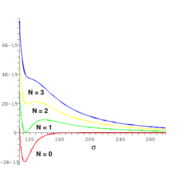
Figure 2: Potential energy of the Kähler modulus in the the original KKLT scenario for $N=0,1,2$ and $3$ antibranes, showing there can be at most 2 antibranes without destabilizing the Kähler modulus.

The situation is dramatically improved if one uses a racetrack superpotential as in ref. KL . The minimum is already Minkowski and adding antibranes in a highly warped throat lifts the vacuum to dS without destabilizing the Kähler modulus. The potential is:

$$V={e^{-2(a+b)\sigma}\over 6\sigma^{2}}(bBe^{a\sigma}+aAe^{b\sigma})$$

$$\times \left[Be^{a\sigma}(3+b\sigma)+e^{b\sigma}(A(3+a\sigma)+3e^{a\sigma}W_{0})\right]+\frac{ND}{\sigma^{3}}$$

where we choose the same parameters as in KL , $A=1,\ B=-1.03,\ a=2\pi/100,\ b=2\pi/99,\ W_{0}=-2\times 10^{-4}$ and $D=10^{-9}$. With these values the critical number of branes turns out to be $N=28$, illustrated in fig. 3

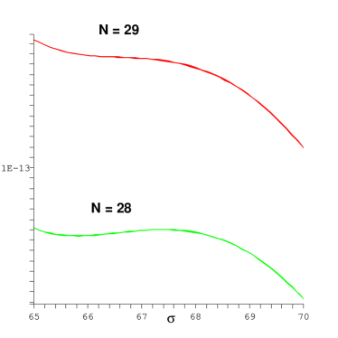
Figure 3: Using a racetrack superpotential and a throat with stronger warping one can add a large number (28 in this example) of antibranes while keeping the Kähler modulus stable.

In the remaining analysis, we will not be concerned with the particular model of Kähler modulus stabilization, beyond the assumption that it admits the required number of additional branes. It will also be found that a large number is not required, so the racetrack model mentioned here is sufficient to establish the existence of a viable model.

III Inflaton Action

Our starting point for the dynamics of inflation is the Lagrangian for the mobile brane position $\psi$ in the IKLIMT framework. To simplify the analysis, we will assume that all moduli (notably the Kähler modulus $\sigma$) are heavy except for the inflaton, and that the 4D effective cosmological constant vanishes at the end of inflation. The Lagrangian can be parametrized as

$${\cal L}={6\sigma\over r^{2}}\dot{\psi}^{2}-{T\epsilon\over r^{2}}\left(1+{\epsilon\over(\psi-\psi_{0})^{4}}\right)^{-1}$$ (3)

where $r=(2\sigma-\psi^{2})$ dWG , $T$ is related to the tension $\tau$ of the 3-brane or antibrane by $T=2\tau/g_{s}^{4}$ KKLT , $\epsilon$ is the warp factor, $\psi$ is the 3-brane position, and $\psi_{0}$ is the location of the antibrane. To keep our work self-contained, this expression is derived in Appendix A, in just the same way as in IKLIMT  except for the omission of two approximations: (1) we do not assume that $\psi\gg\psi_{0}$, and (2) we do not Taylor-expand the term $(1+{\epsilon/(\psi-\psi_{0})^{4}})^{-1}$.

Let us first comment on point (1) above. In IKLIMT and certain other investigations of brane-antibrane inflation, it was assumed that inflation takes place sufficiently far from the antibrane to justify the approximation $|\psi-\psi_{0}|\cong\psi_{0}$. On the other hand, the $\psi_{0}$ parameter was kept in BCSQ and IT . Physically, it may be important to allow for nonzero $\psi_{0}$ because of the possibility that the $\psi$-dependence coming from the $(2\sigma-\psi^{2})^{2}$ factor in the potential will tend to stabilize the brane at some point other than the bottom of the warped throat, in the absence of the brane-antibrane interaction. An example where this is particularly clear is that of two symmetrically placed warped throats, each with its own antibrane IT . In that case the potential (translated to our notation) was taken to be

$$V={T\epsilon\over r^{2}}\left(2-{\epsilon\over(\psi-\psi_{0})^{4}}-{\epsilon\over(\psi+\psi_{0})^{4}}\right)$$ (4)

From symmetry considerations it is obvious in this model that there exists a metastable or unstable equilibrium point exactly midway between the two throats, at $\psi=0$, which cannot coincide with the bottom of either throat. If we simply remove one of the throats, the result corresponds to our starting point (3).

The presence or absence of the $\psi_{0}$ parameter explains differences in the amount of required fine-tuning of the potential found in different investigations. To elucidate this, recall that the $\psi$-dependence in the volume modulus $r=(2\sigma-\psi^{2})$ is the origin of the $\eta$ problem pointed out in IKLIMT—the mass of the inflaton is of order $\sqrt{V}\sim H$ in Planck units, ruining the slow roll condition. It was noticed by BCSQ that it is possible to tune parameters of a model with a potential similar to that in (3) so that the slow-roll conditions are satisfied, even without adding any extra $\psi$-dependent corrections to the superpotential, by varying only the parameters which already appear. However, the degree of tuning needed was more severe than in IKLIMT  where corrections to the superpotential were invoked. One way of understanding this is to realize that if $\psi_{0}=0$ and only corrections of order $\psi^{2}$ are added, then the potential automatically has $V^{\prime}(0)=0$, so that one of the slow roll parameters $V^{\prime}/V$ is small without any tuning. Then only the $\eta$ parameter ($V^{\prime\prime}/V$) needs to be tuned. In our potential however, both slow-roll parameters must be tuned, for generic parameters in the potential. In BCSQ it was found that 60 e-foldings of inflation could be obtained by tuning the warp factor to one part in 2000, whereas IKLIMT only needed one part in 100 tuning. Although this sounds contrary to the spirit of the present paper, it was due to the fact that no systematic study of the effect of varying $\psi_{0}$ was done in BCSQ ; instead only one fixed value was considered.

We note that the behavior of the potential as $\psi\to\psi_{0}$ is classically correct, since by derivation it is of the form $1/h(\psi)$ where $h(\psi)$ satisfies $\nabla^{2}h=C\delta(\psi-\psi_{0})$ in the 6D Calabi-Yau manifold. Although the full brane position must be specified by 3 complex $\psi$ coordinates, we are keeping the angular ones fixed and following only the radial coordinate for the brane-antibrane separation.

We also comment on our choice of avoiding the second approximation (point (2) above), by not Taylor expanding $(1+{\epsilon/(\psi-\psi_{0})^{4}})^{-1}$. We choose not to do so because there is no advantage in making this expansion—it only leads to an unphysical divergence in the potential energy as the brane-antibrane distance shrinks. The unexpanded form has good behavior as $\psi\to\psi_{0}$, including the vanishing of the potential at the minimum.

III.1 Multibrane Lagrangian

We will be interested below in the generalization to more than one brane rolling. The Lagrangian for $N$ branes and $N$ antibranes is

$${\cal L}={6\sigma\over r^{2}}\sum_{i=1}^{N}\dot{\psi}_{i}^{2}-{NT\epsilon\over r^{2}}\left(1+\sum_{i=1}^{N}{\epsilon\over(\psi_{i}-\psi_{0})^{4}}\right)^{-1}$$ (5)

where now the volume modulus is

$$r=2\sigma-\sum_{i=1}^{N}\psi_{i}^{2}$$ (6)

Later we will specialize to the situation where all the branes are coincident, $\psi_{i}=\psi$. Then the potential takes the form $N\epsilon Tr^{-2}(1+N\epsilon(\psi-\psi_{0})^{-4})^{-1}$.

IV Conditions for Inflation

The optimal potential for achieving slow roll inflation is one where both the first and second derivatives vanish simultaneously at some critical point $\psi_{c}$. Although this requires fine tuning, we will discuss a mechanism where the tuning can automatically occur through a dynamical process. To characterize the tuning, we introduce new parameters

$$a = {N\epsilon\over\psi_{0}^{4}},\quad b^{2}={2\sigma\epsilon\over\psi_{0}^{6}},\quad x={\psi\over\psi_{0}}$$ (7)

such that the potential is proportional to

$$\hat{V}(x)={1\over\left({b^{2}/a}-x^{2}\right)^{2}}\,\left(1+{a\over(x-1)^{4}}\right)^{-1}$$ (8)

The conditions for the potential to have a flat point, as defined above, are

$$a=(6x-1)(x-1)^{4},\quad 5x^{2}(x-1)^{4}=b^{2}$$ (9)

These equations can be solved analytically, as the solution of a cubic equation, but the expression is not very enlightening. Instead we give an approximate description, by first considering $b$ as a free parameter, and determining as a function of $b$ the critical values $a_{c}$ and $x_{c}$ which satisfy (9). For consistency, we should also require that $b^{2}\geq a$; otherwise the potential blows up at $x=b/\sqrt{a}<1$, before the brane reaches the antibrane. The range of values where $a_{c}>0$ (obviously also required for a physically sensible solution) and $a_{c}<b^{2}$ turns out to be rather narrow,

$$0.259<b<0.286,$$ (10)

and in this region $a_{c}$ is to a good approximation a linear function of $b$:

$$a_{c}\cong 3b-0.77$$ (11)

One can also approximate the critical value $x_{c}$ by a quadratic form, $x_{c}\cong-0.146+1.21b+6(b-0.259)(b-0.286)$.

We will show later that the narrowness of the interval (10) is an accident, in the sense that physically well-motivated perturbations to the potential can remove this restriction. Therefore we will ultimately not regard it as a fine tuning. However the special value $a_{c}$ for a given value of $b$ clearly does represent a fine tuning of the parameters. It is this condition which will be addressed by a dynamical mechanism. Namely, by starting with a large enough number $N$ of branes, one can initially have $a>a_{c}$ (but still $a<b^{2}$). The potential always has a metastable minimum from which branes can tunnel in this case. After each tunneling event, the value of $a$ diminishes by a discrete amount. At some critical number of branes, $N_{c}$, the curvature changes so that the branes roll instead of being trapped. It becomes a quantitative question, depending on the values of $\sigma$ and $\epsilon$, whether the potential is sufficiently flat to give enough inflation. We will show that in fact it is almost always flat enough to give at least 60 e-foldings of inflation.

To find out how likely it is that adequate inflation will occur, we have explored the parameter space $\epsilon,\ \sigma,\ b$, subject to the aforementioned restrictions and the assumption that $N$ starts out being larger than the critical value, where all the branes start to roll. For each value of $\{\epsilon,\ \sigma,\ b\}$, the quantities $\psi_{0}$ and $N_{c}$ are determined. The fields start from rest at the value where the potential has a local minimum with $N=N_{c}+1$ branes, on the assumption that the nontunneling branes do not move during the tunneling event. The equations of motion are

$${d\pi_{i}\over dt}=-3H\pi_{i}-{\partial V\over\partial\psi_{i}},\quad{dN_{e}\over dt}=H$$ (12)

for the canonical momentum

$$\pi_{i}={12\sigma\over r^{2}}\dot{\psi}_{i}$$ (13)

and number of e-foldings $N_{e}\equiv\ln a(t)$, where the Hubble parameter is given by $H^{2}=(6\sigma N\dot{\psi}^{2}/r^{2}+V)/(3M_{p}^{2})$. Since all the fields move together, we need consider only one equation for the inflatons, which we do numerically.

The result is that, for $b$ satisfying (10), there is a high probability of getting enough inflation, for random values of $\epsilon,\sigma$ selected from within a reasonable range, $-5\leq\log_{10}\epsilon\leq-2.4$, $1\leq\log_{10}2\sigma\leq 3.6$. Scanning uniformly over this region, we find that $85\%$ of tries result in more than 55 e-foldings of inflation when $b=0.27$, and an even greater percentage occurs for other values of $b$. The results are illustrated for $b=0.27$ in Figure 4, showing the number of e-foldings, $N_{e}$ (omitting values where $N_{e}>300$ for clarity) versus $\log_{10}\epsilon$ and $\log_{10}2\sigma$.

In figure 4 it can be seen that $N_{e}$ is constant along lines of constant $A\equiv(2\sigma)^{2/3}\epsilon^{-1/3}$. This can be understood by rewriting the potential in terms of the canonically normalized field $\phi=\psi_{i}\sqrt{3N/\sigma}$:

$$V={T\,N\over A^{3}}\left(1-\frac{1}{6}\phi^{2}\right)^{-2}\left(1-{36(N/A)^{3}\over(\phi-\phi_{0})^{4}}\right)^{-1}$$ (14)

where $\phi_{0}=b^{-1/3}\sqrt{3N/A}$. Thus for fixed $b$, the shape of the potential, power spectrum, and duration of inflation depend only upon combination of parameters in $A$, and not on the orthogonal combination $B=(2\sigma)^{1/3}\epsilon^{2/3}$. We can therefore restrict our exploration of parameter space to a one-dimensional scan along the direction of $A$. Moreover, we can show that the number of branes $N$ depends in a very simple way on the value of $A$: $N=ab^{-4/3}A$. This follows from eliminating $\psi_{0}$ from the definitions of $a$ and $b$. Therefore the critical number of branes is given by

$$N_{c}=a_{c}\,b^{-4/3}\,{(2\sigma)^{2/3}\over\epsilon^{1/3}}$$ (15)

and for a fixed value of $b$, we can treat the parameters $A$ and $N_{c}$ interchangeably. Of course (15) can’t be satisfied exactly, because $N_{c}$ has to be an integer. The accidental discrepancies between the optimal value of $N_{c}$ and the closest integer below this value will affect how long inflation actually lasts.

Figure 4: $N_{e}$ versus $\log_{10}\epsilon$ and $\log_{10}2\sigma$ for $b=0.27$, in the range $N_{e}<300$.

In figure 5 we show the correlation between number of e-foldings and the critical number of branes, scanning uniformly in the interval $1<\log_{10}A<4$ of parameter space. Although the two quantities are generally correlated, there are order-of-magnitude variations in $N_{e}$ over narrow ranges of $N_{c}$. Figure 5 demonstrates that both features can be matched fairly well by an empirical relationship. Let $\Delta N_{c}$ be the discrepancy between the ideal value of $N_{c}$ and the closest integer below this value. Then we find that

$$N_{e}\cong 10{\sqrt{N_{c}}\over\Delta N_{c}}$$ (16)

The factor $1/\Delta N_{c}$, is understandable since if $\Delta N_{c}=0$, the potential is tuned to be perfectly flat at some position $\psi=\psi_{c}$.

Figure 5: $\log N_{e}$ versus the critical number of branes $\log N_{c}$, $b=0.27$. The empirical relationship (16) is also plotted.

The factor $\sqrt{N_{c}}$ in (16) can be partly understood in terms of assisted inflation assisted . With $N$ fields rolling simultaneously, the kinetic term is multiplied by $N$ relative to one field. We should rescale the fields by $\psi\to\psi/\sqrt{N}$, and the slow-roll parameters by $1/N$. One therefore expects an enhancement in the length of inflation by some power of $N_{c}$. It would of course be satisfying to understand why that power is $1/2$ in the present model. We have not yet succeeded in analytically deriving this result. However it is not surprising that $N_{e}$ fails to be enhanced by a full factor of $N_{c}$ as would be the case for ordinary assisted inflation, because the potential contains $N\psi^{2}$ in the Kähler modulus. Only if the potential was independent of $N$ would we be sure that $N_{e}\sim N_{c}$. In that case, transforming to the canonically normalized field would cause $V(\psi)\to V(\phi/\sqrt{N})$ and the slow roll parameters would go like $\eta\sim V^{\prime\prime}/V\sim 1/N$. The surprise is that there is any assisted inflation effect at all. The reason for it is that at the critical value of $N$, the potential is flatter than it would generically be for an arbitrary function of $N\psi^{2}$.

The above results were for $b=0.27$. Allowing $b$ to vary, ones finds that smaller $b$ tends to give more inflation with a smaller number of branes. This dependence is shown in figure 6. The main observation, though, is that the great majority of all cases yield more than $60$ e-foldings of inflation.

Figure 6: $\log N_{e}$ versus $\log N_{c}$ for $b=0.26,\ 0.27,$ and $0.28$.

V Scalar Power Spectrum

In addition to having a long enough period of inflation, we must obtain a spectrum of density perturbations in agreement with observational constraints from the Cosmic Microwave Background. To compute the power spectrum, we use the following expression SS which applies to a set of noncanonically normalized fields with Lagrangian ${\cal L}=\frac{1}{2}G_{ij}\dot{\psi}^{i}\dot{\psi}^{j}-V$:

$$P(k)={V\over 75\pi^{2}M_{p}^{2}}{\partial N_{e}\over\partial\psi^{i}}{\partial N_{e}\over\partial\psi^{j}}G^{ij}={N_{c}VH^{2}\over 75\pi^{2}M_{p}^{2}}\,{r\over 6\dot{\psi}^{2}}$$ (17)

These quantities are evaluated at horizon crossing of the relevant wave number, when $k=aH$. To normalize the spectrum, we evaluate $P(k)$ for modes which crossed the horizon 55 e-foldings before inflation ended, corresponding to a scale of inflation around $V^{1/4}\sim 4\times 10^{14}$ GeV. The consistency of this assumption will be verified. The COBE normalization implies that $P\cong 4\times 10^{-10}$ for these modes. This allows us to normalize the scale of the potential by fixing the value of the parameter $T$ which is proportional to the unwarped brane tension. The results are expressed in terms of the scale of inflation relative to the Planck scale. In figure 7 we plot $\log(V^{1/4}/M_{p})$ as a function of the number of branes. (In the previous section it was explained that, just like $N_{e}$, spectral properties depend only on the same combination of $\sigma$ and $\epsilon$ which determine $N_{c}$.) From the figure one sees that the inflationary scale ranges between $10^{-3}$ and $10^{-4.5}M_{p}$, roughly consistent with our assumption of $\sim 55$ e-foldings of inflation. The string scale, which determines the brane tension, must be in about the same range. If the number of branes is small enough, the inflationary scale can be sufficiently high for the tensor contribution to the cosmic microwave background to be observable in future experiments.

Figure 7: Log of the inflationary scale as a function of the number of branes.

The scalar spectral index is given by $n_{s}=1+d\ln P/d\ln k$. We have numerically evaluated it over the relevant range of parameters. Like the other quantities, it is most conveniently displayed as a function of the number of branes. The deviation $n_{s}-1$ at 55 e-foldings before the end of inflation is shown as a function of $N_{c}$ in figure 8. There is a wide range of possible values, $-0.07<n_{s}-1<0.15$.

Figure 8: Deviation of scalar spectral index from unity versus $N_{c}$

It is also interesting to consider the running of the spectral index, $dn/d\ln k=d^{2}\ln P/d\ln k^{2}$, for which WMAP has given a hint of a larger-than-expected negative value, $dn/d\ln k\cong-0.02$ WMAP-inf . Although the error bars are large enough to be consistent with no running, the suggestion of large running has attracted attention. Generically, within the slow-roll formalism, one expects $dn/d\ln k\sim(n_{s}-1)^{2}$, which is usually smaller than the measured central value. Our numerical survey shows that it is possible to have rare instances of running as negative as $-0.01$, even though inflation lasts long enough. However, as shown in figure 9, it is still true that $dn/d\ln k\sim(n_{s}-1)^{2}$. The rare cases of large running correspond to occasional extreme values of the spectral index.

We have checked that the spectral index and running are in good agreement with the predictions of slow roll inflation, $n-1=2\eta-6\varepsilon$, $dn/d\ln k=-2\xi+16\epsilon\eta-24\varepsilon^{2}$, where $\varepsilon=\frac{1}{2}(V^{\prime}/V)^{2}$, $\eta=V^{\prime\prime}/V$ and $\xi=V^{\prime}V^{\prime\prime\prime}/V^{2}$, in units where $M_{p}=1$. The derivatives must be taken with respect to the canonically normalized fields, $\phi_{i}=(r/\sqrt{12\sigma})\psi_{i}$. In all cases, $\varepsilon\sim 10^{-6}-10^{-9}$, whereas $\eta\sim-0.03$ and $\xi\sim 10^{-3}$. The running is completely dominated by $\xi$.

Figure 9: $dn/d\ln k$ versus $n_{s}$.

It is interesting to compare the predicted values of the running and the spectral index with experimental constraints from combined WMAP and Sloan Digital Sky Survey Lyman $\alpha$ data Seljak The allowed region is superimposed on the predictions in figure 10. Although most of the predicted points are allowed, we note that the few examples with large running have too large a deviation of $n_{s}$ from unity. Thus if large running should be experimentally confirmed in the future, it will rule out the models under consideration.

Figure 10: $dn/d\ln k$ with $n-1$, with WMAP$+$SDSS constraints shown.

VI Generalized Models

The previous analysis shows that within a narrow range of the parameter $b=\sqrt{2\sigma\epsilon}/\psi_{0}^{3}$, a long period of inflation will always ensue, as long as the initial number of mobile branes exceeded the critical number $N_{c}$. But since $b$ looks fine-tuned, this is not a complete solution to the problem of naturalness for the inflaton potential. Could this be an accident of the particular form of the simplest IKLIMT potential? To answer this, we explore the effect of perturbing the model by corrections which are expected to be present, but which we have so far ignored for the sake of simplicity.

At least two kinds of modifications to the basic IKLIMT model are generically expected: corrections to the superpotential and to the Kähler potential. A simple example of the former was considered in KKLMMT , where the superpotential for the Kähler modulus $T=\sigma+i\theta$ and inflaton was taken to be

$$W=W_{0}+g(T)(1+\delta\psi^{2})$$ (18)

leading to a contribution to the potential of the form

$$\delta V={\alpha+\beta\psi^{2}+\gamma\psi^{4}\over(2\sigma-\psi^{2})^{2}}$$ (19)

with $\sigma$-dependent coefficients $\alpha,\ \beta,\ \gamma$. This should be added to the brane-antibrane potential which we have been using so far. In the case of $N$ branes, we take $W=W_{0}+g(T)(1+\delta\sum_{i}\psi_{i}^{2})$. To simplify the analysis, we consider examples where $\alpha,\ \beta,\ \gamma$ are chosen in such a way that the full potential continues to have a global minimum at $\psi=\psi_{0}$, where $V(\psi_{0})$ is assumed to vanish:

$$\delta V\sim N\delta{(\psi^{2}-\psi_{0}^{2})^{2}\over(2\sigma-N\psi^{2})^{2}}$$ (20)

We have included the factors of $N$ appropriate to the multibrane case, when all branes are coincident.

The second kind of correction involves the Kähler potential, which for $N$ branes was taken to be $K=-3\ln(T+\bar{T}-\sum_{i}|\psi_{i}|^{2})$ dWG . This was always understood to be an approximate expression, good when $\psi_{i}^{2}\ll\sigma$, but subject to higher order corrections in $\psi_{i}$, for example $|\psi_{i}|^{4}$. The denominator in $V+\delta V$ would then be replaced by

$$(2\sigma-N\psi^{2})^{2}\to(2\sigma-N(\psi^{2}+d\psi^{4}))^{2}$$ (21)

As shown in Appendix B, the Kähler corrections also give contributions to the numerator of the F-term potential, whose Taylor series starts with a term of order $\psi^{4}$. For small $\psi$, we can absorb this leading term into the $\gamma$ coefficient of (19). The kinetic term ${\cal K}_{a\bar{b}}\dot{\phi}^{a}\dot{\bar{\phi}}^{b}$ also gets ${\cal O}(d\psi^{2})$ corrections, which can be inferred from eq. (47), but these are negligible whenever the branes are slowly rolling.

By the above reasoning, the two kinds of corrections enter into the rescaled potential (8) as

$$\hat{V}\to{1\over\left({b^{2}\over a}-x^{2}-dx^{4}\right)^{2}}\,\left(c(x^{2}-1)^{2}+\left(1+{a\over(x-1)^{4}}\right)^{-1}\right)$$ (22)

By experimenting with this generalized potential, one finds that the new coefficient $c$ allows for the removal of the lower bound on $b$ in (10). Moreover, negative values of $d$ can remove the upper bound. It is easy to find values of $c$ and $d$ for which the potential has the desired behavior as a function of $N$, as in figure 1, regardless of the value of $b$. For example $c=0.1$, $d=-0.5$ yields the potentials shown in figure 11, at $b=0.01$ and $b=5$. It is important that the new parameters $c$ and $d$ are independent of the number of branes. Thus $a$ continues to be the only parameter which changes due to a brane tunneling event.

Figure 11: Rescaled brane-antibrane potential (22) including Kähler and superpotential corrections.

As in the previous section, we scanned over parameters for which $A$ varies, hence the number of branes, while keeping $b,\ c,\ d$ fixed, for the two examples with $b=0.01$ and $b=5$. Figure 12 shows the number of e-foldings versus number of branes. The general growth of $N_{e}\sim\sqrt{N_{c}}$ is evident, as it was for the simple model of the previous section.

Figure 12: Log of number of e-foldings versus log of the critical number of branes, for the examples illustrated in figure 9.

Figure 13 shows the correlation of $dn/d\ln k$ with $n_{s}$. It shows that the small-$b$ model tends to have a red spectrum, with $n_{s}<1$, and negligible running. The large-$b$ model also has $n_{s}<1$ for most realizations, but for rare cases with $N\mbox{\raisebox{-2.58334pt}{~{}$\stackrel{{\scriptstyle<}}{{\sim}}$~{}}}20$, it is possible to get large deviations from a flat spectrum with $n_{s}>1$. These are accompanied by sizable running, but as in figure 10, such points occur outside of the experimentally allowed region. The overall conclusion is that the generalized models have similar qualitative behavior to the simplest class which was studied in sections III-IV.

Figure 13: $dn/d\ln k$ versus $n_{s}$ for the models with Kähler and superpotential corrections.

VII Caveats and Conclusions

In this work we have presented a very general means whereby a long period of inflation, with a suitably flat spectrum of density perturbations, can be automatically obtained after tunneling of branes, from a metastable position in a Calabi-Yau manifold, into a warped throat containing antibranes. It depends only on the fact that the brane-antibrane potential generically has such a metastable minimum when the number of branes is sufficiently large, and the possibility of starting at a place in the string theory landscape where the number of mobile branes exceeds the threshold for having a minimum. Once a certain critical number of branes $N_{c}$ is reached, the minimum disappears and the branes start rolling slowly to the true minimum. They automatically start from the same position, which is guaranteed to be close to the flattened region of the potential.

In this scenario, an arbitrarily long time will be spent in a metastable de Sitter phase resembling old inflation, before the slow rolling period (similarly to ref. new-old ). Each tunneling event results in a small bubble of open universe, within which another period of quasi-de Sitter expansion will occur. The process repeats itself until the critical number of branes is reached. For us, these long periods of old inflation are irrelevant—we have focused entirely on the final phase of conventional inflation associated with the smooth motion of the branes until they annihilate with antibranes in the throat, hopefully leading to the reheating of the universe reheating , and perhaps the production of cosmic superstrings cosmic-string .

We numerically scanned over large ranges of the logarithm of relevant combinations of parameters which govern the shape of the inflaton potential, and found that large fractions ($\sim 10-90\%$) of the trials resulted in inflation with no need for tuning, whenever the flattening mechanism could occur. This seems to be a quite promising approach for ameliorating the need for fine-tuning within the framework of the string-theory landscape landscape .

For convenience of numerical integration, we chose a form of the potential which has good behavior as the branes reach the bottom of the throat. This form, which differs from the commonly used Taylor-expanded form, is in fact the result of a direct perturbative computation, and does not require any special assumptions. However, the perturbative derivation does assume that $N\epsilon/(\psi-\psi_{0})^{4}\ll 1$ in order to be valid. One might therefore wonder how sensitive our results are to the behavior of the potential when this approximation is breaking down. We have investigated what happens if the Taylor expansion $1-N\epsilon/(\psi-\psi_{0})^{4}$ is used in place of $(1+N\epsilon/(\psi-\psi_{0})^{4})^{-1}$, and we also checked different ways of regulating the singularity, like $1-N\epsilon/(N\epsilon+(\psi-\psi_{0})^{4})$. For all these alternatives, we found that although the specific parameter values where a flat potential occurs may be somewhat sensitive to the behavior of the potential near $\psi_{0}$, the mechanism of multibrane inflation nevertheless works in the same way as we have presented. We therefore believe it to be a robust result, which is qualitatively quite different from field theory models of inflation.

Although the dynamical flattening of the potential requires a rather special range of parameters in the simplest IKLIMT model, we showed that this restriction can be lifted once corrections to the superpotential and the Kähler potential are taken into account. We exhibited an example of such corrections that works, without systematically exploring the parameter space of such corrections. Subjectively, it seems that the parameter space (referred to as $\{b,c\}$ in section V) where multibrane inflation works will be large, given that it was easy to find a successful example, but a more complete investigation could be made. Moreover, such corrections should in principle be computed from a fully string theoretic starting point, which might restrict the allowed ranges of $\{b,c\}$.

Another issue which deserves further study is the precise relationship between the radial coordinate $r$ of the brane within the warped throat, and the field $\psi$ which is used to describe the inflaton position in the supergravity description. The exact correspondence between these fields was not needed in IKLIMT because the main dependence on $\psi$ was taken to be through the Kähler modulus factor (and superpotential corrections), rather than a combination of these with the brane-antibrane potential. We have simply identified the two fields in our analysis, but the actual relation could be more complicated, possibly introducing additional parameters into the Lagrangian.

Appendix A Brane-Antibrane Potential in Warped Throat

We consider the background of $AdS_{5}\times X_{5}$ space with the $AdS_{5}$ metric:

$$ds_{5}^{2}=\frac{r^{2}}{R^{2}}\left(-dt^{2}+d{\bf x}^{2}\right)+\frac{R^{2}}{r^{2}}dr^{2}$$ (23)

where $R^{4}=4\pi ag_{s}N{\alpha^{\prime}}^{2}$ is the radius of the $AdS_{5}$ space created as the near-horizon geometry of a stack of $N\gg 1$ $D3$ branes. There is also an $RR$ background field created by the stack of branes:

$$A_{x^{0},x^{1},x^{2},x^{3}}=\lim_{r\rightarrow 0}\frac{1}{1+\left(\frac{R}{r}\right)^{4}}\simeq\left(\frac{r}{R}\right)^{4}$$ (24)

If one now writes the action for a probe brane is this background, one finds:

$$S_{D3} = -T_{3}\int d^{4}\xi\sqrt{-\det\left(\partial_{\xi^{a}}x^{M}\partial_{\xi^{b}}x^{N}g_{NM}\right)}$$ (25)

$$+ T_{3}\int d^{4}\xi A_{x^{0},x^{1},x^{2},x^{3}}$$

We will use the convention that $\xi^{0}=t$, but the rest of the coordinates will describe the location of the brane, including fluctuations (local bendings), $x^{i}=x^{i}\left(\xi^{0},\xi^{i}\right)=x^{i}\left(t,\xi^{i}\right)$. We make here a further assumption, namely that only its radial location varies.

$$\partial_{\xi^{a}}x^{M}\partial_{\xi^{b}}x^{N}g_{NM}=\partial_{\xi^{a}}x^{0}\partial_{\xi^{b}}x^{0}g_{00}+\partial_{\xi^{a}}x^{i}\partial_{\xi^{b}}x^{i}g_{ii}+\partial_{\xi^{a}}r\partial_{\xi^{b}}rg_{rr}$$ (26)

The metric will look like:

$$\left(\begin{array}[]{cccc}g_{00}+g_{rr}\left(\frac{\partial r}{\partial\xi^{0}}\right)^{2}&g_{rr}\frac{\partial r}{\partial\xi^{0}}\frac{\partial r}{\partial\xi^{1}}&g_{rr}\frac{\partial r}{\partial\xi^{0}}\frac{\partial r}{\partial\xi^{2}}&g_{rr}\frac{\partial r}{\partial\xi^{0}}\frac{\partial r}{\partial\xi^{3}}\\ g_{rr}\frac{\partial r}{\partial\xi^{1}}\frac{\partial r}{\partial\xi^{0}}&g_{xx}+g_{rr}\left(\frac{\partial r}{\partial\xi^{1}}\right)^{2}&g_{rr}\frac{\partial r}{\partial\xi^{1}}\frac{\partial r}{\partial\xi^{2}}&g_{rr}\frac{\partial r}{\partial\xi^{1}}\frac{\partial r}{\partial\xi^{3}}\\ g_{rr}\frac{\partial r}{\partial\xi^{2}}\frac{\partial r}{\partial\xi^{0}}&g_{rr}\frac{\partial r}{\partial\xi^{2}}\frac{\partial r}{\partial\xi^{1}}&g_{yy}+g_{rr}\left(\frac{\partial r}{\partial\xi^{2}}\right)^{2}&g_{rr}\frac{\partial r}{\partial\xi^{2}}\frac{\partial r}{\partial\xi^{3}}\\ g_{rr}\frac{\partial r}{\partial\xi^{3}}\frac{\partial r}{\partial\xi^{0}}&g_{rr}\frac{\partial r}{\partial\xi^{3}}\frac{\partial r}{\partial\xi^{1}}&g_{rr}\frac{\partial r}{\partial\xi^{3}}\frac{\partial r}{\partial\xi^{2}}&g_{zz}+g_{rr}\left(\frac{\partial r}{\partial\xi^{3}}\right)^{2}\end{array}\right)=\left(\begin{array}[]{cccc}g_{00}&0&0&0\\ 0&g_{xx}&0&0\\ 0&0&g_{yy}&0\\ 0&0&0&g_{zz}\end{array}\right)+\left(g_{rr}\frac{\partial r}{\partial\xi^{\mu}}\frac{\partial r}{\partial\xi^{\nu}}\right)$$ (27)

We can apply the usual formula:

$$\det\left(A+\epsilon B\right)=\det A\det\left(1+\epsilon A^{-1}B\right)\simeq\det A\left(1+\epsilon\;Tr\left(A^{-1}B\right)\right)$$ (28)

Writing the metric at the location of the brane as: $g_{\mu\nu}=\frac{r^{2}}{R^{2}}f_{\mu\nu}$ we obtain:

$$\det\left(\partial_{\xi^{a}}x^{M}\partial_{\xi^{b}}x^{N}g_{NM}\right)=-\left(\frac{r}{R}\right)^{8}\left(1-\left(\frac{R}{r}\right)^{4}\!\!f^{\mu\nu}\frac{\partial r}{\partial\xi^{\mu}}\frac{\partial r}{\partial\xi^{\nu}}\right)$$ (29)

The factor $\frac{r^{4}}{R^{4}}$ in the bracket comes from the product

$$g^{\mu\nu}g_{rr}=\left(\frac{R}{r}\right)^{4}f^{\mu\nu}$$ (30)

Using these results in the $DBI+CS$ action we obtain:

$$S_{D3} = -T_{3}\int d^{4}\xi\sqrt{-f}\left(\frac{r}{R}\right)^{4}\sqrt{1-\left(\frac{R}{r}\right)^{4}\!\!\!f^{\mu\nu}\frac{\partial r}{\partial\xi^{\mu}}\frac{\partial r}{\partial\xi^{\nu}}}$$ (31)

$$\pm T_{3}\int d^{4}\xi\det\left(\frac{\partial x}{\partial\xi}\right)\left(\frac{r}{R}\right)^{4}\epsilon_{t\xi^{1}\xi^{2}\xi^{3}}$$

Expanding the square root term we obtain for a $D3$ brane (sign $+$):

$$S_{D3}=T_{3}\int d^{4}\xi\sqrt{-f}\frac{1}{2}f^{\mu\nu}\frac{\partial r}{\partial\xi^{\mu}}\frac{\partial r}{\partial\xi^{\nu}}$$ (32)

while for a $\overline{D}3$ (sign $-$):

$$S_{\overline{D}3} = T_{3}\int d^{4}\xi\sqrt{-f}\frac{1}{2}f^{\mu\nu}\frac{\partial r}{\partial\xi^{\mu}}\frac{\partial r}{\partial\xi^{\nu}}$$ (33)

$$- 2T_{3}\int d^{4}\xi\sqrt{-f}\left(\frac{r}{R}\right)^{4}$$

The extra piece in the case of the $\overline{D}3$ comes from the non-BPS nature of the antibrane, since the graviton exchange and the RR exchange forces now add instead of canceling (for 3-branes the dilaton is constant and contributes no force). The potential energy for the $\overline{D}3$ in the gravitational + RR field will make it favorable for the brane to move towards $r=0$, that is, the bottom of the $AdS_{5}$ throat. For the setup in fig.(14) we have to add the piece corresponding to the graviton + RR exchange between the $D3$ and the $\overline{D}3$.

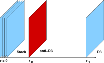
Figure 14: IKLIMT setup

However in this setup we have to include the effect of the $D3$ in addition to that of the stack. The derivation of the background perturbed by the presence of the $D3$ placed away from the stack can be found in Appendix B of IKLIMT. It starts by writing the metric in the form:

$$ds_{10}^{2} = h^{-\frac{1}{2}}\left(-dt^{2}+d{\bf x}^{2}\right)+h^{\frac{1}{2}}\left(dr^{2}+\frac{r^{2}}{R^{2}}\overline{g}_{ab}dy^{a}dy^{b}\right)$$

$$h = \frac{R^{4}}{r^{4}}$$ (34)

placing the extra $D3$ brane at $r_{1}$ and solving for the perturbed harmonic function

$$h\left(r\right)=\frac{R^{4}}{r^{4}}+\delta h\left(r\right)$$ (35)

which satisfies the Laplace equation in the space transverse to the brane, which is spanned by $r$ and $y^{a}$:

$$\nabla^{2}_{\left(6\right)}\delta h\left(r\right)=C\delta^{\left(6\right)}\left(\vec{r}-\vec{r}_{1}\right)$$ (36)

which amounts to solving:

$$\frac{R^{5}}{r^{5}}\partial_{r}\left[\frac{r^{5}}{R^{5}}\partial_{r}\delta h\left(r\right)\right]=C\delta^{\left(6\right)}\left(\vec{r}-\vec{r}_{1}\right)$$ (37)

which give $\delta h\left(r\right)\sim|\vec{r}-\vec{r}_{1}|^{-4}$. A similar equation is satisfied by the unperturbed $h$. The constants $C$ and $C^{\prime}$ depend on the total “charge”, more precisely the total tension of the brane or stack of branes, so they are related by:

$$C=\frac{C^{\prime}}{N}$$ (38)

and since the solution for the unperturbed $h\left(r\right)$ is already known, we can immediately find the solution for $\delta h\left(r\right)$

$$\delta h\left(r\right)=\frac{C}{|\vec{r}-\vec{r}_{1}|^{4}}=\frac{R^{4}}{N}\cdot\frac{1}{|\vec{r}-\vec{r}_{1}|^{4}}$$ (39)

We can use the perturbed metric to calculate the action for the $\overline{D}3$ using the new function $h\left(r\right)+\delta h\left(r\right)$.

Now modify the setup and place at $r_{0}$ a stack of $M$ $\overline{D}3$’s with $M\ll N$ and an equal number of $D3$’s placed at $r_{1},r_{2}\dots r_{M}$, as shown in figure 15. We can simply generalize the analysis above to come to the result:

$$h\left(r\right)=\frac{R^{4}}{r^{4}}+\frac{R^{4}}{N}\cdot\sum_{j=1}^{M}\frac{1}{|\vec{r}-\vec{r}_{j}|^{4}}$$ (40)

There is no interaction between the $D3$’s or between the $\overline{D}3$’s in the second stack since they are mutually BPS. We can now go back to eq. (31) and replace the expression $R^{4}/r^{4}$ by $h\left(r\right)$. The relevant term is the second term from eq. (33), which in the limit $r_{i}\gg r$ becomes:

$$2T_{3}\int d^{4}\xi\sqrt{-f}\frac{1}{h\left(r\right)}=2T_{3}\int d^{4}\xi\sqrt{-f}\frac{r_{0}^{4}}{R^{4}}\cdot\frac{1}{1+\frac{r_{0}^{4}}{N}\sum_{j=1}^{M}\frac{1}{r_{j}^{4}}}\cong\int d^{4}\xi\sqrt{-f}\left\{2T_{3}\cdot\frac{r_{0}^{4}}{R^{4}}\cdot\left(1-\frac{1}{N}\sum_{j=1}^{M}\frac{r_{0}^{4}}{r_{j}^{4}}\right)\right\}$$ (41)

where $r_{0}$ is the location of the stack of antibranes. The above result is for one single $\overline{D}3$ in the stack. The final form of the effective action should be multiplied by $M$, the number of antibranes in the stack.

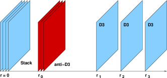
Figure 15: Modified setup

Appendix B Kähler potential corrections

The Kähler potential is assumed to have the following form:

$$K=-3\log\left(r\right)=-3\log\left(T+\overline{T}-f\left(\phi_{i},\overline{\phi}_{i}\right)\right)$$ (42)

and we will also assume that $f$ decomposes into a sum of functions, each one depending on one field $\phi_{i}$:

$$K=-3\log\left(T+\overline{T}-\sum_{i}f_{i}\left(\phi_{i},\overline{\phi}_{i}\right)\right)$$ (43)

The simplest form of the functions $f_{i}$ is

$$f_{i}\left(\phi_{i},\overline{\phi}_{i}\right)=\phi_{i}\overline{\phi}_{i}$$ (44)

but we can consider more complicated expressions, for example:

$$f_{i}\left(\phi_{i},\overline{\phi}_{i}\right)=\phi_{i}\overline{\phi}_{i}-\left(\phi_{i}\overline{\phi}_{i}\right)^{2}$$ (45)

Allowing for the more complicated expression for $f_{i}\left(\phi_{i},\overline{\phi}_{i}\right)$ changes the structure of the singularities of the Kähler potential and of the F-term.

In the general case the Kähler metric derived from the Kähler potential of eq. (43) has the form:

$${\mathcal{K}}_{a\overline{b}}=\frac{3}{r^{2}}\left(\begin{array}[]{ccccc}1&-\frac{\partial f_{1}}{\partial\phi_{1}}&-\frac{\partial f_{2}}{\partial\phi_{2}}&\cdots&-\frac{\partial f_{n}}{\partial\phi_{n}}\\ -\frac{\partial f_{1}}{\partial\phi_{1}^{*}}&\frac{\partial f_{1}}{\partial\phi_{1}}\frac{\partial f_{1}}{\partial\phi_{1}^{*}}+r\frac{\partial^{2}f_{1}}{\partial\phi_{1}\partial\phi_{1}^{*}}&\frac{\partial f_{1}}{\partial\phi_{1}^{*}}\frac{\partial f_{2}}{\partial\phi_{2}}&\cdots&\frac{\partial f_{1}}{\partial\phi_{1}^{*}}\frac{\partial f_{n}}{\partial\phi_{n}}\\ \vdots&\vdots&\vdots&\ddots&\vdots\\ -\frac{\partial f_{n-1}}{\partial\phi_{n-1}^{*}}&\frac{\partial f_{n-1}}{\partial\phi_{n-1}^{*}}\frac{\partial f_{1}}{\partial\phi_{1}}&\frac{\partial f_{n-1}}{\partial\phi_{n-1}^{*}}\frac{\partial f_{2}}{\partial\phi_{2}}&\cdots&\frac{\partial f_{n-1}}{\partial\phi_{n-1}^{*}}\frac{\partial f_{n}}{\partial\phi_{n}}\\ -\frac{\partial f_{n}}{\partial\phi_{n}^{*}}&\frac{\partial f_{n}}{\partial\phi_{n}^{*}}\frac{\partial f_{1}}{\partial\phi_{1}}&\frac{\partial f_{n}}{\partial\phi_{n}^{*}}\frac{\partial f_{2}}{\partial\phi_{2}}&\cdots&\frac{\partial f_{n}}{\partial\phi_{n}^{*}}\frac{\partial f_{n}}{\partial\phi_{n}}+r\frac{\partial^{2}f_{n}}{\partial\phi_{n}\partial\phi_{n}^{*}}\end{array}\right)$$ (46)

The inverse can also be calculated:

$${\mathcal{K}}^{\overline{a}b}=\frac{r}{3}\left(\begin{array}[]{ccccc}r+\frac{\partial f_{1}}{\partial\phi_{1}}\frac{\partial f_{1}}{\partial\phi_{1}^{*}}/\frac{\partial^{2}f_{1}}{\partial\phi_{1}\partial\phi_{1}^{*}}+\dots+\frac{\partial f_{n}}{\partial\phi_{n}}\frac{\partial f_{n}}{\partial\phi_{n}^{*}}/\frac{\partial^{2}f_{n}}{\partial\phi_{n}\partial\phi_{n}^{*}}&\frac{\partial f_{1}}{\partial\phi_{1}^{*}}/\frac{\partial^{2}f_{1}}{\partial\phi_{1}\partial\phi_{1}^{*}}&\frac{\partial f_{2}}{\partial\phi_{2}^{*}}/\frac{\partial^{2}f_{2}}{\partial\phi_{2}\partial\phi_{2}^{*}}&\ldots&\frac{\partial f_{n}}{\partial\phi_{n}^{*}}/\frac{\partial^{2}f_{n}}{\partial\phi_{n}\partial\phi_{n}^{*}}\\ \frac{\partial f_{1}}{\partial\phi_{1}}/\frac{\partial^{2}f_{1}}{\partial\phi_{1}\partial\phi_{1}^{*}}&1/\frac{\partial^{2}f_{1}}{\partial\phi_{1}\partial\phi_{1}^{*}}&0&\ldots&0\\ \frac{\partial f_{2}}{\partial\phi_{2}}/\frac{\partial^{2}f_{2}}{\partial\phi_{2}\partial\phi_{2}^{*}}&0&1/\frac{\partial^{2}f_{2}}{\partial\phi_{2}\partial\phi_{2}^{*}}&\ldots&0\\ \vdots&\vdots&\vdots&\ddots&\vdots\\ \frac{\partial f_{n}}{\partial\phi_{n}}/\frac{\partial^{2}f_{n}}{\partial\phi_{n}\partial\phi_{n}^{*}}&0&0&\ldots&1/\frac{\partial^{2}f_{n}}{\partial\phi_{n}\partial\phi_{n}^{*}}\end{array}\right)$$ (47)

The F-term is calculated using the usual formula:

$$V_{F}=e^{\mathcal{K}}\left(K^{\overline{a}b}\overline{D_{a}W}D_{b}W-3\left|W\right|^{2}\right)$$ (48)

where

$${\mathcal{K}}=-3\log\left(r\right)$$ (49)

The covariant derivatives are expressed as:

$$D_{T}W = \partial_{T}W+W\partial_{T}{\mathcal{K}}=\partial_{T}W-\frac{3}{r}W$$ (50)

$$D_{\phi_{i}}W = \partial_{\phi_{i}}W+W\partial_{\phi_{i}}{\mathcal{K}}=\frac{\partial f_{i}}{\partial\phi_{i}}\frac{3}{r}W$$ (51)

$$\overline{D_{T}W} = \partial_{\overline{T}}\overline{W}+\overline{W}\partial_{\overline{T}}{\mathcal{K}}=\partial_{\overline{T}}\overline{W}-\frac{3}{r}\overline{W}$$ (52)

$$\overline{D_{\phi_{i}}W} = \partial_{\overline{\phi_{i}}}\overline{W}+\overline{W}\partial_{\overline{\phi_{i}}}{\mathcal{K}}=\frac{\partial f_{i}}{\partial\phi_{i}^{*}}\frac{3}{r}\overline{W}$$ (53)

Using the above expression for the inverse Kähler metric one obtains the following terms:

$$K^{\overline{T}T}\overline{D_{T}W}D_{T}W = \frac{r}{3}\left(\partial_{\overline{T}}\overline{W}-\frac{3}{r}\overline{W}\right)\left(\partial_{T}W-\frac{3}{r}W\right)\left(r+\frac{\frac{\partial f_{1}}{\partial\phi_{1}}\frac{\partial f_{1}}{\partial\phi_{1}^{*}}}{\frac{\partial^{2}f_{1}}{\partial\phi_{1}\partial\phi_{1}^{*}}}+\dots+\frac{\frac{\partial f_{n}}{\partial\phi_{n}}\frac{\partial f_{n}}{\partial\phi_{n}^{*}}}{\frac{\partial^{2}f_{n}}{\partial\phi_{n}\partial\phi_{n}^{*}}}\right)$$ (54)

$$K^{\overline{T}\phi_{i}}\overline{D_{T}W}D_{\phi_{i}}W = \frac{r}{3}\left(\partial_{\overline{T}}\overline{W}-\frac{3}{r}\overline{W}\right)W\left(\frac{3}{r}\frac{\partial f_{1}}{\partial\phi_{1}}\frac{\frac{\partial f_{1}}{\partial\phi_{1}^{*}}}{\frac{\partial^{2}f_{1}}{\partial\phi_{1}\partial\phi_{1}^{*}}}+\dots+\frac{3}{r}\frac{\partial f_{n}}{\partial\phi_{n}}\frac{\frac{\partial f_{n}}{\partial\phi_{n}^{*}}}{\frac{\partial^{2}f_{n}}{\partial\phi_{n}\partial\phi_{n}^{*}}}\right)$$ (55)

$$K^{\overline{\phi_{i}}T}\overline{D_{\phi_{i}}W}D_{T}W = \frac{r}{3}\left(\partial_{T}W-\frac{3}{r}W\right)\overline{W}\left(\frac{3}{r}\frac{\partial f_{1}}{\partial\phi_{1}^{*}}\frac{\frac{\partial f_{1}}{\partial\phi_{1}}}{\frac{\partial^{2}f_{1}}{\partial\phi_{1}\partial\phi_{1}^{*}}}+\dots+\frac{3}{r}\frac{\partial f_{n}}{\partial\phi_{n}^{*}}\frac{\frac{\partial f_{n}}{\partial\phi_{n}}}{\frac{\partial^{2}f_{n}}{\partial\phi_{n}\partial\phi_{n}^{*}}}\right)$$ (56)

$$K^{\overline{\phi_{i}}\phi_{j}}\overline{D_{\phi_{i}}W}D_{\phi_{j}}W = \frac{r}{3}W\overline{W}\left(\frac{9}{r^{2}}\frac{\partial f_{1}}{\partial\phi_{1}}\frac{\partial f_{1}}{\partial\phi_{1}^{*}}\frac{1}{\frac{\partial^{2}f_{1}}{\partial\phi_{1}\partial\phi_{1}^{*}}}+\dots+\frac{9}{r^{2}}\frac{\partial f_{n}}{\partial\phi_{n}}\frac{\partial f_{n}}{\partial\phi_{n}^{*}}\frac{1}{\frac{\partial^{2}f_{n}}{\partial\phi_{n}\partial\phi_{n}^{*}}}\right)$$ (57)

Adding all the above terms and $-3\left|W\right|^{2}$ we obtain the F-term:

$$V_{F}=\frac{1}{r^{3}}\left[\frac{r^{2}}{3}\partial_{\overline{T}}\overline{W}\partial_{T}W\left(1+\frac{\frac{\partial f_{1}}{\partial\phi_{1}}\frac{\partial f_{1}}{\partial\phi_{1}^{*}}}{r\frac{\partial^{2}f_{1}}{\partial\phi_{1}\partial\phi_{1}^{*}}}+\dots+\frac{\frac{\partial f_{n}}{\partial\phi_{n}}\frac{\partial f_{n}}{\partial\phi_{n}^{*}}}{r\frac{\partial^{2}f_{n}}{\partial\phi_{n}\partial\phi_{n}^{*}}}\right)-r\left(W\partial_{\overline{T}}\overline{W}+\overline{W}\partial_{T}W\right)\right]$$ (58)

We assumed that the superpotential itself is independent of the fields $\phi_{1}\dots\phi_{n}$.

References

- (1) G. R. Dvali and S. H. H. Tye, “Brane inflation,” Phys. Lett. B 450, 72 (1999) [arXiv:hep-ph/9812483]. C. P. Burgess, M. Majumdar, D. Nolte, F. Quevedo, G. Rajesh and R. J. Zhang, “The inflationary brane-antibrane universe,” JHEP 0107, 047 (2001) [arXiv:hep-th/0105204]. J. Garcia-Bellido, R. Rabadan and F. Zamora, “Inflationary scenarios from branes at angles,” JHEP 0201, 036 (2002) [arXiv:hep-th/0112147]. C. P. Burgess, P. Martineau, F. Quevedo, G. Rajesh and R. J. Zhang, “Brane antibrane inflation in orbifold and orientifold models,” JHEP 0203, 052 (2002) [arXiv:hep-th/0111025]. R. Blumenhagen, B. Kors, D. Lust and T. Ott, “Hybrid inflation in intersecting brane worlds,” Nucl. Phys. B 641, 235 (2002) [arXiv:hep-th/0202124]. N. Jones, H. Stoica and S. H. H. Tye, “Brane interaction as the origin of inflation,” JHEP 0207, 051 (2002) [arXiv:hep-th/0203163]. K. Dasgupta, C. Herdeiro, S. Hirano and R. Kallosh, “D3/D7 inflationary model and M-theory,” Phys. Rev. D 65, 126002 (2002) [arXiv:hep-th/0203019]. O. DeWolfe, S. Kachru and H. L. Verlinde, “The giant inflaton,” JHEP 0405, 017 (2004) [arXiv:hep-th/0403123]. J. J. Blanco-Pillado et al., “Racetrack inflation,” JHEP 0411, 063 (2004) [arXiv:hep-th/0406230]. E. Silverstein and D. Tong, “Scalar speed limits and cosmology: Acceleration from D-cceleration,” Phys. Rev. D 70, 103505 (2004) [arXiv:hep-th/0310221]. M. Alishahiha, E. Silverstein and D. Tong, “DBI in the sky,” Phys. Rev. D 70, 123505 (2004) [arXiv:hep-th/0404084]. X. g. Chen, “Multi-throat brane inflation,” Phys. Rev. D 71, 063506 (2005) [arXiv:hep-th/0408084]; “Inflation from warped space,” arXiv:hep-th/0501184. K. Becker, M. Becker and A. Krause, “M-theory inflation from multi M5-brane dynamics,” Nucl. Phys. B 715, 349 (2005) [arXiv:hep-th/0501130].
- (2) S. Kachru, R. Kallosh, A. Linde, J. Maldacena, L. McAllister and S. P. Trivedi, “Towards inflation in string theory,” JCAP 0310, 013 (2003) [arXiv:hep-th/0308055].
- (3) S. B. Giddings, S. Kachru and J. Polchinski, “Hierarchies from fluxes in string compactifications,” Phys. Rev. D 66, 106006 (2002) [arXiv:hep-th/0105097].
- (4) I. R. Klebanov and M. J. Strassler, “Supergravity and a confining gauge theory: Duality cascades and SB-resolution of naked singularities,” JHEP 0008, 052 (2000) [arXiv:hep-th/0007191].
- (5) S. Kachru, R. Kallosh, A. Linde and S. P. Trivedi, “De Sitter vacua in string theory,” Phys. Rev. D 68, 046005 (2003) [arXiv:hep-th/0301240].
- (6) S. P. de Alwis, “Effective potentials for light moduli,” arXiv:hep-th/0506266.
- (7) C. P. Burgess, J. M. Cline, H. Stoica and F. Quevedo, “Inflation in realistic D-brane models,” JHEP 0409, 033 (2004) [arXiv:hep-th/0403119].
- (8) M. Berg, M. Haack and B. Kors, “Loop corrections to volume moduli and inflation in string theory,” Phys. Rev. D 71, 026005 (2005) [arXiv:hep-th/0404087]. L. McAllister, “An inflaton mass problem in string inflation from threshold corrections to volume stabilization,” arXiv:hep-th/0502001.
- (9) D. Cremades, F. Quevedo and A. Sinha, “Warped tachyonic inflation in type IIB flux compactifications and the open-string completeness conjecture,” arXiv:hep-th/0505252.
- (10) J. P. Hsu, R. Kallosh and S. Prokushkin, “On brane inflation with volume stabilization,” JCAP 0312, 009 (2003) [arXiv:hep-th/0311077]. J. P. Hsu and R. Kallosh, “Volume stabilization and the origin of the inflaton shift symmetry in string theory,” JHEP 0404, 042 (2004) [arXiv:hep-th/0402047]. H. Firouzjahi and S. H. H. Tye, “Closer towards inflation in string theory,” Phys. Lett. B 584, 147 (2004) [arXiv:hep-th/0312020].
- (11) H. Firouzjahi and S. H. Tye, “Brane inflation and cosmic string tension in superstring theory,” JCAP 0503, 009 (2005) [arXiv:hep-th/0501099].
- (12) R. Kallosh and A. Linde, “Landscape, the scale of SUSY breaking, and inflation,” JHEP 0412, 004 (2004) [arXiv:hep-th/0411011].
- (13) O. DeWolfe and S. B. Giddings, “Scales and hierarchies in warped compactifications and brane worlds,” Phys. Rev. D 67, 066008 (2003) [arXiv:hep-th/0208123]. S. B. Giddings and A. Maharana, “Dynamics of warped compactifications and the shape of the warped landscape,” arXiv:hep-th/0507158.
- (14) N. Iizuka and S. P. Trivedi, Phys. Rev. D 70, 043519 (2004) [arXiv:hep-th/0403203].
- (15) A. R. Liddle, A. Mazumdar and F. E. Schunck, “Assisted inflation,” Phys. Rev. D 58, 061301 (1998) [arXiv:astro-ph/9804177]. A. Mazumdar, S. Panda and A. Perez-Lorenzana, “Assisted inflation via tachyon condensation,” Nucl. Phys. B 614, 101 (2001) [arXiv:hep-ph/0107058]. Y. S. Piao, R. G. Cai, X. m. Zhang and Y. Z. Zhang, “Assisted tachyonic inflation,” Phys. Rev. D 66, 121301 (2002) [arXiv:hep-ph/0207143].
- (16) M. Sasaki and E. D. Stewart, “A General analytic formula for the spectral index of the density perturbations produced during inflation,” Prog. Theor. Phys. 95, 71 (1996) [arXiv:astro-ph/9507001].
- (17) H. V. Peiris et al., “First year Wilkinson Microwave Anisotropy Probe (WMAP) observations: Implications for inflation,” Astrophys. J. Suppl. 148, 213 (2003) [arXiv:astro-ph/0302225].
- (18) U. Seljak et al., “Cosmological parameter analysis including SDSS Ly-alpha forest and galaxy bias: Constraints on the primordial spectrum of fluctuations, neutrino mass, and dark energy,” Phys. Rev. D 71, 103515 (2005) [arXiv:astro-ph/0407372].
- (19) G. Dvali and S. Kachru, “New old inflation,” arXiv:hep-th/0309095.
- (20) J. M. Cline, H. Firouzjahi and P. Martineau, “Reheating from tachyon condensation,” JHEP 0211, 041 (2002) [arXiv:hep-th/0207156]. N. Barnaby and J. M. Cline, “Creating the universe from brane-antibrane annihilation,” Phys. Rev. D 70, 023506 (2004) [arXiv:hep-th/0403223]. N. Barnaby, C. P. Burgess and J. M. Cline, “Warped reheating in brane-antibrane inflation,” JCAP 0504, 007 (2005) [arXiv:hep-th/0412040]. L. Kofman and P. Yi, “Reheating the universe after string theory inflation,” arXiv:hep-th/0507257.
- (21) S. Sarangi and S. H. H. Tye, “Cosmic string production towards the end of brane inflation,” Phys. Lett. B 536, 185 (2002) [arXiv:hep-th/0204074]. N. T. Jones, H. Stoica and S. H. H. Tye, “The production, spectrum and evolution of cosmic strings in brane inflation,” Phys. Lett. B 563, 6 (2003) [arXiv:hep-th/0303269]. L. Pogosian, S. H. H. Tye, I. Wasserman and M. Wyman, “Observational constraints on cosmic string production during brane inflation,” Phys. Rev. D 68, 023506 (2003) [arXiv:hep-th/0304188]. E. J. Copeland, R. C. Myers and J. Polchinski, “Cosmic F- and D-strings,” JHEP 0406, 013 (2004) [arXiv:hep-th/0312067]. T. Damour and A. Vilenkin, “Gravitational radiation from cosmic (super)strings: Bursts, stochastic background, and observational windows,” Phys. Rev. D 71, 063510 (2005) [arXiv:hep-th/0410222].
- (22) N. Barnaby, A. Berndsen, J. M. Cline and H. Stoica, “Overproduction of cosmic superstrings,” JHEP 0506, 075 (2005) [arXiv:hep-th/0412095].
- (23) L. Susskind, “The anthropic landscape of string theory,” arXiv:hep-th/0302219. T. Banks, M. Dine and E. Gorbatov, “Is there a string theory landscape?,” JHEP 0408, 058 (2004) [arXiv:hep-th/0309170].