Abstract

Codimension-two objects on a system of brane-antibrane are studied in the context of Born-Infeld type effective field theory with a complex tachyon and U(1)$\times$U(1) gauge fields. When the radial electric field is turned on in D2${\bar{\rm D}}$2, we find static regular global and local D-vortex solutions which could be candidates of straight cosmic D-strings in a superstring theory. A natural extension to DF-strings is briefly discussed.

1 Introduction and Model

Cosmic strings arise as vortices in field theories, mainly when either global or gauge U(1) symmetry is spontaneously broken. The point-like vortices in 2-dimensional space become long straight strings in 3-dimensional space simply by stretching them along the extra-spatial direction with maintaining the 2-dimensional field configurations independent of the straight third spatial coordinate. Thus, if these straight strings are gravitating, it is almost the same as gravitating the point-like vortices in planar gravity, which results in conic geometry at asymptote. These static properties of cosmic strings constitute a main basis for studying formation and evolution of straight and wiggly cosmic strings and their networks, which could be left as cosmological fossils at the present Universe [1, 2].

Since almost all of the ideas from vortices in local gauge theories with Higgs mechanism can carry over to superstrings, it seems natural to consider macroscopic superstring as a candidate of cosmic strings. This possibility was firstly taken into account in Ref. [3]. However, it was excluded by the following reasons as production of large inhomogeneity in the cosmic microwave background, dilution of string density through inflation, and instability to keep long strings. Development of D-branes during the last decade encourages us to tackle again this issue with cosmic D- and DF-strings [4, 5, 6] and the related topics [7, 8, 9].

For the description of D- and DF-strings, an efficient approach is to employ the method of effective field theory from string theory. As stated in the first paragraph, the first step for constructing cosmic D- and DF-strings in the context of effective field theory is to find point-like vortex solutions in the plane, particularly static and regular solutions [10, 11, 12]. In the scheme of effective field theory, instability of brane-antibrane system is represented by a complex tachyon field $(T,\bar{T})$, and this tachyon is indispensable for the generation of topological defects. Since this system possesses U(1)$\times$U(1) gauge symmetry, we need two gauge fields, $A^{a}_{\mu},\;a=1,2$. Separation of the brane and the antibrane is described by scalar fields $X^{I}_{a}$ corresponding to the transverse coordinates of individual branes. Among various proposed tachyon effective actions [13, 14], we shall deal with Dirac-Born-Infeld (DBI) type effective action of the D$p{\bar{\rm D}}p$ system in Ref. [15],

$$S = -{\cal T}_{p}\int d^{p+1}x\,V(T,X^{I}_{1}-X^{I}_{2})$$ (1.1)

$$\hskip 42.67912pt\times\left\{\,\sqrt{-\det\left[g_{\mu\nu}+F_{\mu\nu}^{1}+\partial_{\mu}X^{I}_{1}\partial_{\nu}X^{I}_{1}+({\overline{D_{\mu}T}}D_{\nu}T+{\overline{D_{\nu}T}}D_{\mu}T)/2\right]}\right.$$

$$\hskip 56.9055pt\left.+\sqrt{-\det\left[g_{\mu\nu}+F_{\mu\nu}^{2}+\partial_{\mu}X^{I}_{2}\partial_{\nu}X^{I}_{2}+({\overline{D_{\mu}T}}D_{\nu}T+{\overline{D_{\nu}T}}D_{\mu}T)/2\right]}\,\,\right\},$$

where ${\cal T}_{p}$ is the tension of the D$p$-brane, $F_{\mu\nu}^{a}=\partial_{\mu}A^{a}_{\nu}-\partial_{\nu}A^{a}_{\mu}$, and $D_{\mu}T=(\partial_{\mu}-iA_{\mu}^{1}+iA^{2}_{\mu})T$. For small tachyon amplitude $\tau$ from $T=\tau e^{i\chi}$, behavior of the tachyon potential is

$$V(T,X^{I}_{1}-X^{I}_{2})=1-\left[\frac{1}{R^{2}}-\sum_{I}(X^{I}_{1}-X^{I}_{2})^{2}\right]\tau^{2}+{\cal O}(\tau^{4}),$$ (1.2)

where $R$ is $\sqrt{2}$ in superstring theory.

In the context of DBI-type effective action describing D-brane systems with instability, there have been much study on codimension-one solitons (codimension-one branes), particularly tachyon kinks [16, 15, 17, 18, 19]. For vortices (codimension-two branes), only the singular local vortex solution with finite energy was constructed from the DBI action (1.1) [15], and regular tachyon vortex solutions were obtained in local field theory action with quadratic derivative terms and polynomial tachyon potential [20, 10, 14, 4].

It is well-known that fundamental strings attached to a D-brane becomes flux tube solutions (spikes or BIons) with nonzero thickness in nonlocal field theory of DBI-action [21]. Thickness of a tachyon kink becomes nonzero when the constant DBI electric field transverse to the codimension-one D-brane is tuned on, and, it becomes, at its critical value, thick static regular BPS tachyon kink [17, 19]. In this paper, we show that both global and local D-vortices have zero-thickness without DBI electric field, but global and local D-vortices with electric flux become regular with nonzero thickness. These regular configurations are interpreted as a nonzero size D0 on D2${\bar{\rm D}}$2 on which fundamental strings are attached.

In section 2, without a U(1) gauge field, we discuss static singular global D-vortex configuration with zero radial electric field and static regular global D-vortex with nonzero radial electric field. In section 3, with a U(1) gauge field, we find the singular and regular local D-vortex solutions. Section 4 involves discussions on RR-charge and extension of D-vortices to straight stringy objects in D3${\bar{\rm D}}$3 system. We conclude in section 5 with summary of the obtained results and discussions for further study.

2 Global D-Vortices

Let us consider D$p{\bar{\rm D}}p$ system in the coincidence limit of two branes, $X^{I}_{1}=X^{I}_{2}$, with fundamental strings. Then the macroscopic fundamental strings in fluid state are represented by electric fluxes along their directions. Vortex-like codimension-two objects of our interest could be interpreted as D$(p-2)$-branes. For description of the global vortex-like objects, the gauge fields and their field strengths should behave as $A_{\mu}^{1}=A_{\mu}^{2}=A_{\mu}$ and $F_{\mu\nu}^{1}=F_{\mu\nu}^{2}=F_{\mu\nu}$ in the action (1.1). Then the action (1.1) in (1+$p$)-dimensions becomes

$$S=-2{\cal T}_{p}\int d^{p+1}x\,V(\tau)\sqrt{-\det X}\,,$$ (2.1)

where

$$X_{\mu\nu}=g_{\mu\nu}+F_{\mu\nu}+(\partial_{\mu}{\bar{T}}\partial_{\nu}T+\partial_{\nu}{\bar{T}}\partial_{\mu}T)/2.$$ (2.2)

Additionally we assume that the produced D$(p-2)$-branes are flat and all the transverse degrees are frozen. Then we can neglect dependence of the transverse coordinates and it is enough to find D0-branes from flat D$2{\bar{\rm D}}2$. In the context of solitons in the effective theory, it is translated as point-like vortices on a plane. We will call this vortex as D-vortex in what follows.

When dependence of the transverse scalar fields $X^{I}_{a}$ disappears in (1.2), the tachyon potential $V$ is invariant under the exchange symmetry of the brane and antibrane and coincides with that of an unstable D$p$-brane [22]. Since it measures varying tension of the ${\rm D2}\bar{{\rm D}}2$ system and then universality allows any runaway tachyon potential connecting the following two boundary values smoothly and monotonically [23]

$$V(\tau=0)=1\quad{\rm and}\quad V(\tau=\infty)=0$$ (2.3)

which has a ring of degenerate minima at infinite tachyon amplitude. We will use a specific potential [24, 25] for the analysis for vortex solutions

$$V(\tau)=\frac{1}{{\rm cosh}\left(\frac{\tau}{R}\right)},$$ (2.4)

but the obtained results are the same under the assumption of any symmetric tachyon potential, $V(\tau)=V(-\tau)$, satisfying (2.3) with $V(\tau)\sim e^{-\tau/R}$ for large $\tau$ [26]. Note that soliton solutions have been firstly investigated under the action with quadratic derivative kinetic term and runaway potential in the context of quintessence [27].

2.1 Singular global D-vortex

The simplest D-vortex configuration is that of static $n$ vortices superimposed at a point. It is convenient to use radial coordinates $(t,r,\theta)$ with $g_{\mu\nu}={\rm diag}(-1,1,r^{2})$ and to choose the vortex point as the origin $r=0$. Ansatz for the $n$ superimposed vortices is

$$T(r,\theta)=\tau(r)e^{in\theta},$$ (2.5)

and that for D-vortices require vanishing $F_{\mu\nu}$. Substituting these into the effective action (2.1), we have

$$\frac{S}{\int d^{p-2}x_{\perp}}=-2{\cal T}_{p}\int dtdrd\theta rV(\tau)\sqrt{\left(1+\tau^{{}^{\prime}2}\right)\left(1+\frac{n^{2}}{r^{2}}\tau^{2}\right)}\,,$$ (2.6)

where ^′ denotes $d/dr$.

When we have a topological D-vortex solution of vorticity $n$, the tachyon amplitude is given by a monotonic increasing function connecting the following boundary values smoothly. The boundary condition at the origin is forced by the ansatz (2.5)

$$\tau(r=0)=0,\qquad(n\neq 0),$$ (2.7)

and that at infinity is read from runaway nature of the tachyon potential (2.3)–(2.4)

$$\tau(r\rightarrow\infty)\rightarrow\infty.$$ (2.8)

First of all, we verify nonexistence of regular global D-vortex solution satisfying the boundary conditions (2.7)–(2.8) by examining the tachyon equation from the action (2.6):

$$\frac{1}{r}\frac{d}{dr}\left[\frac{rV}{\sqrt{X}}\left(1+\frac{\tau^{2}}{r^{2}}n^{2}\right)~{}\tau^{\prime}\right]-\frac{V}{\sqrt{X}}(1+\tau^{{}^{\prime}2})\tau\frac{n^{2}}{r^{2}}=\sqrt{X}~{}\frac{dV}{d\tau},$$ (2.9)

where

$$X=\left(1+\tau^{{}^{\prime}2}\right)\left(1+\frac{n^{2}\tau^{2}}{r^{2}}\right).$$ (2.10)

Physical properties are read from non-vanishing components of the energy-momentum tensor

$$T^{t}_{\;t} = -\frac{2{\cal T}_{p}V}{\sqrt{X}}\left[\left(1+\tau^{\prime 2}\right)\left(1+\frac{n^{2}}{r^{2}}\tau^{2}\right)\right],$$ (2.11)

$$T^{r}_{\;r} = -\frac{2{\cal T}_{p}V}{\sqrt{X}}\left(1+\frac{n^{2}}{r^{2}}\tau^{2}\right),$$ (2.12)

$$T^{\theta}_{\;\theta} = -\frac{2{\cal T}_{p}V}{\sqrt{X}}\left(1+\tau^{\prime 2}\right).$$ (2.13)

Suppose that there exists single topological tachyon vortex solution of vorticity $n$ ($\neq 0$), satisfying the boundary conditions (2.7)–(2.8). We try a power-series and a logarithmic solution for sufficiently large $r$, assuming each leading behavior of the tachyon amplitude is

$$\tau(r)\approx\left\{\begin{array}[]{ll}\displaystyle{\tau_{\infty}r^{k}}&\qquad(k\geq 0),\\ \displaystyle{\tau_{\infty}{\rm ln}r}&.\end{array}\right.$$ (2.14)

Inserting it into the tachyon equation (2.9), we have an approximate equation from the leading terms

$$\left\{\begin{array}[]{ll}\displaystyle{C_{k}r^{-k}\approx-\frac{1}{R}}&C_{k}=0~{}\mbox{for}~{}k>1,\\ \displaystyle{\frac{(1-n^{2})\tau_{\infty}}{1+n^{2}\tau_{\infty}^{2}}\frac{1}{r}\approx-\frac{1}{R}}&\mbox{for}~{}k=1~{}\mbox{and}~{}n\neq 1,\\ \displaystyle{-\frac{\tau_{\infty}^{2}}{R}\approx-\frac{1+\tau_{\infty}^{2}}{R}}&\mbox{for}~{}k=1~{}\mbox{and}~{}n=1,\\ \displaystyle{\tau_{\infty}(k^{2}-n^{2})r^{p-2}\approx-\frac{1}{R}}&\mbox{for}~{}0<k<1,\\ \displaystyle{-n^{2}\tau_{\infty}\frac{\ln r}{r^{2}}\approx-\frac{1}{R}}&\mbox{for}~{}\tau(r)\approx\tau_{\infty}\ln r.\end{array}\right.$$ (2.15)

All five cases in the left-hand and right-hand sides of (2.15) lead to contradiction. An exponentially growing $\tau(r)$ for sufficiently large $r$ also turns out to arrive at contradiction. Thus, there does not exist static regular single global topological vortex connecting $\tau(r=0)=0$ and $\tau(r=\infty)=\infty$ monotonically. Note that the proof of nonexistence holds for all the tachyon potentials only if $V(\tau)\sim e^{-\tau/R}$ for large $\tau$.

This phenomenon of nonexistence seems familiar since it also appears in tachyon kinks and tachyon tubes where the form of static regular solutions are given by array of kink-antikink or array of tube-antitube [16, 17, 18, 28] instead of single kink or single tube. Despite of the nonexistence of regular single tachyon kink, the constructed singular single tachyon kink configuration [15] was reconciled as zero thickness limit of a single BPS kink part of the array [17, 18, 29].

Following the wisdom of boundary string field theory of D2${\bar{\rm D}}$2-system [13], let us try a linear tachyon configuration with infinite slope, $\tau(r)=r/\epsilon,~{}~{}\epsilon\rightarrow 0$. Then pressure components (2.12)–(2.13) have the same value even at the origin, $T^{r}_{\;r}(0)=T^{\theta}_{\;\theta}(0)=-2{\cal T}_{2}$ and $T^{r}_{\;r}(r\neq 0)=T^{\theta}_{\;\theta}(r\neq 0)=0$, and the conservation law of energy-momentum tensor equivalent to the tachyon equation (2.9) becomes simple in the limit of $\epsilon\rightarrow 0$: $T^{r^{\prime}}_{\;r}+T^{r}_{\;r}/r-T^{\theta}_{\;\theta}/r=T^{r^{\prime}}_{\;r}=0$. This nonvanishing pressure implies that the obtained singular D-vortex may not be a BPS object and it is different from the cases of thin kink [16, 17] or thin tube [29], where transverse pressure vanishes $T_{xx}=0$. Energy density $-T^{t}_{\;t}$ (2.11) is peaked at the origin like a $\delta$-function and the corresponding tension of the thin D0-brane is given the following decent relation

$$2{\cal T}_{0}^{g} \equiv \int_{0}^{2\pi}d\theta\int_{0}^{\infty}dr\,r(-T^{t}_{\;t})$$ (2.16)

$$\stackrel{{\scriptstyle\tau=r/\epsilon}}{{\approx}} 2(2\sqrt{\pi K}R)^{2}{\cal T}_{2}.$$ (2.17)

The Catalan’s constant $K$ is almost unity, $K\equiv\int_{0}^{\infty}dyy/2{\rm cosh}y\approx 0.91596...$, and so it implies that the decent relation (2.17) is not exact even in the limit of zero thickness, i.e., $2\sqrt{\pi K}/\pi=1.0799...$ means about 8$\%$ error.

2.2 Regular global D-vortex with electric flux

Let us take into account D2${\bar{\rm D}}$2 with fundamental strings of which transverse length is zero in the coincidence limit of the D2${\bar{\rm D}}$2, i.e., $X^{I}_{1}=X^{I}_{2}$ in (1.1)–(1.2). When the location of the fundamental strings coincides with the center of global vortex at the origin $(r=0)$, existence of the fundamental string is marked by non-vanishing radial component of electric field $F_{0r}=E_{r}(r)$ on each D2 (or ${\bar{\rm D}}$2) as shown in Fig. 1. For simplicity we turn off other components of the field strength, $F_{0\theta}=0$ and $F_{r\theta}=0$.

Figure 1: D2 and ${\bar{\rm D}}2$ with fundamental strings represented by $F_{0r}=E_{r}(r)$ in the coincidence limit of $X^{I}_{1}=X^{I}_{2}$. Both the D-vortex and fundamental string are superimposed at the origin ($r=0$).

Substitution of these into the determinant of (2.1) gives the action

$$\frac{S}{\int d^{p-2}x_{\perp}}=-2{\cal T}_{p}\int dtdrd\theta rV(\tau)\sqrt{X}\,,$$ (2.18)

where, with $g\equiv{\rm det}g_{\mu\nu}$,

$${\rm det}\left[g_{\mu\nu}+F_{\mu\nu}+(\partial_{\mu}\bar{T}\partial_{\nu}T+\partial_{\nu}\bar{T}\partial_{\mu}T)/2\right] \equiv gX$$ (2.19)

$$= -r^{2}\left[\left(1-E_{r}^{2}+\tau^{{}^{\prime}2}\right)\left(1+\frac{n^{2}}{r^{2}}\tau^{2}\right)\right].$$ (2.20)

From the action (2.18), tachyon equation of motion is given by

$$\frac{1}{r}\frac{d}{dr}\left[\frac{rV}{\sqrt{X}}\left(1+\frac{\tau^{2}}{r^{2}}n^{2}\right)~{}\tau^{\prime}\right]-\frac{V}{\sqrt{X}}(1+\tau^{{}^{\prime}2}-E_{r}^{2})\tau\frac{n^{2}}{r^{2}}=\sqrt{X}~{}\frac{dV}{d\tau}.$$ (2.21)

The gauge field strength $F_{0r}=E_{r}(r)$ with other components vanishing automatically satisfies Bianchi identity, $\partial_{\mu}F_{\nu\rho}+\partial_{\nu}F_{\rho\mu}+\partial_{\rho}F_{\mu\nu}=0$. Then equation for the gauge field leads to constancy of the conjugate momentum $\Pi^{r}$ multiplied by $r$

$$(r\Pi^{r})^{{}^{\prime}}=0\quad\mbox{for}\quad r\neq 0,$$ (2.22)

where the conjugate momenta for the gauge field $A_{r}$ is

$$\Pi^{r}\equiv\frac{1}{\sqrt{-g}}\frac{\delta S}{\delta(\partial_{t}A_{r})}=\frac{1}{\sqrt{-g}}\frac{\delta S}{\delta F_{tr}}=\frac{2{\cal T}_{p}V}{\sqrt{X}}\left(1+\frac{n^{2}}{r^{2}}\tau^{2}\right)E_{r}(r).$$ (2.23)

Now we obtain an expression for the electric field from the gauge equation (2.22) with (2.23)

$$E_{r}^{2}(r)=\frac{1+\tau^{\prime 2}}{1+\left(\frac{2{\cal T}_{p}V}{\Pi^{r}}\right)^{2}\left(1+\frac{n^{2}}{r^{2}}\tau^{2}\right)},$$ (2.24)

and thereby the only equation to solve is the tachyon equation (2.21). Note that non-vanishing component of conservation of the energy-momentum tensor, $\nabla_{\mu}T^{\mu\nu}=0$, is only the radial component,

$$\frac{d}{dr}\left[\frac{V}{\sqrt{X}}\left(1+\frac{n^{2}}{r^{2}}\tau^{2}\right)\right]+\frac{V}{r\sqrt{X}}\left(E_{r}^{2}+\frac{n^{2}}{r^{2}}\tau^{2}-\tau^{{}^{\prime}2}\right)=0,$$ (2.25)

which is consistent with the tachyon equation (2.21).

Let us try to find asymptotic solution. If the tachyon amplitude approaches infinity with showing power-law behavior $\tau\sim\tau_{\infty}r^{k}$ ($k>0$), $1-E_{r}^{2}+\tau^{{}^{\prime}2}$ and $X$ would be exponentially suppressed due to the factor $V^{2}$ ($\sim 4{\rm exp}[-2\tau_{\infty}r^{k}/R]$). When $0<k<1$ and $k>1$, one can easily notice mismatches between power-law behavior in the left-hand side of (2.25) and exponentially-decreasing behavior in the right-hand side as follows,

$$\left\{\begin{array}[]{cc}k>1:&\frac{(k-1)}{\tau_{\infty}k}r^{-k}\\[5.69054pt] 0<k<1:&\tau_{\infty}k(k-1)r^{k-2}\end{array}\right\}\approx 0~{}~{}{\rm exponentially},$$ (2.26)

Neglecting $V^{2}$, the tachyon equation Eq. (2.21) becomes much simpler,

$$\frac{d}{dr}\left[\frac{\tau^{{}^{\prime}}rV}{\sqrt{X}}\left(1+\frac{n^{2}\tau^{2}}{r^{2}}\right)\right]\approx 0,$$ (2.27)

and the solution of constant $\tau^{{}^{\prime}}$ with $\tau\sim\tau_{\infty}r$ is allowed as a leading behavior. Specifically, $\tau(r)$ and $E_{r}^{2}(r)$ are

$$\tau(r) \approx \tau_{\infty}r+\delta-\frac{4{\cal T}_{p}^{2}R}{\tau_{\infty}^{2}Q_{\rm F1}^{2}}(1+\tau_{\infty}^{2})(1+n^{2}\tau_{\infty}^{2})r^{2}e^{-2\frac{\tau_{\infty}r+\delta}{R}}+{\cal O}(re^{-2\frac{\tau_{\infty}r+\delta}{R}}),$$ (2.28)

$$E_{r}^{2}(r) \approx (1+\tau_{\infty}^{2})\left\{1-\frac{16{\cal T}_{p}^{2}R}{\tau_{\infty}Q_{\rm F1}^{2}}\left[1+n^{2}\tau_{\infty}^{2}\left(1+\frac{2\delta}{R}\right)\right]re^{-2\frac{\tau_{\infty}r+\delta}{R}}+{\cal O}(e^{-2\frac{\tau_{\infty}r+\delta}{R}})\right\},$$ (2.29)

where the constants, $\tau_{\infty}$ ($>0$) and $\delta$, cannot be determined by the information at asymptotic region alone. Unlike the case of single topological BPS tachyon kink [17], the electric field does not approach critical value but a different value in order to make the determinant (2.20) vanish at infinity.

Near the origin consistent power series expansion leads to increasing $\tau$ and decreasing $E_{r}^{2}$ as

$$\tau(r) \approx \tau_{0}r\left[1+\frac{2{\cal T}_{p}^{2}}{3Q_{{\rm F}1}^{2}}(1+\tau_{0}^{2})(n^{2}-1)r^{2}-{\cal O}(r^{4})\right],$$ (2.30)

$$E_{r}^{2}(r) \approx (1+\tau_{0}^{2})\left[1-\frac{4{\cal T}_{p}^{2}}{Q_{{\rm F}1}^{2}}(1+\tau_{0}^{2})r^{2}+{\cal O}(r^{4})\right],$$ (2.31)

where $Q_{{\rm F}1}$ is charge of the fundamental string from (2.22)

$$\Pi^{r}\equiv\frac{Q_{{\rm F1}}}{r}.$$ (2.32)

Numerical solution connecting the behavior near the origin (2.30) and that for large $r$ (2.28) is shown in Fig. 2-(a). Since the coefficient of $r^{3}$-term in (2.30) is positive for $n\geq 2$ but that of $r^{5}$-term in (2.30) is negative for $n=1$, $\tau$ for $n=2$ is convex-up near the origin but that for $n=1$ is convex-down (See Fig. 2-(a)). Though the string charge density $\Pi^{r}$ (2.32) has singularity at the origin, the corresponding electric field $E_{r}$ is regular as shown in (2.31) (See Fig. 2-(b)). From the graphs Fig. 2-(a) and (b), we read the values of $\tau_{\infty}$, $\tau_{\infty}=4.41$ for $n=1$ and $\tau_{\infty}=6.02$ for $n=2$, which satisfy the consistency condition $E_{r}^{2}(\infty)\approx 1+\tau^{2}(\infty)$. The leading behavior of tachyon is dominated by linear term near the origin (2.28) and at infinity (2.30) irrespective of the vorticity $n$ although values of the coefficients are different, i.e., $\tau_{0}\neq\tau_{\infty}$ from Fig. 2-(a). This phenomenon is different from that of the vortices in local field theory models, and possibly is a reflection of the string theory: In boundary string field theory, D0-brane obtained from D2${\bar{\rm D}}$2-system has been analyzed by employing a linear configuration of which BPS limit is achived in the limit of infinite slope [13].

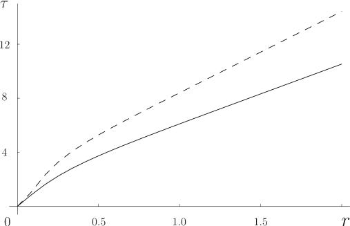
(a)

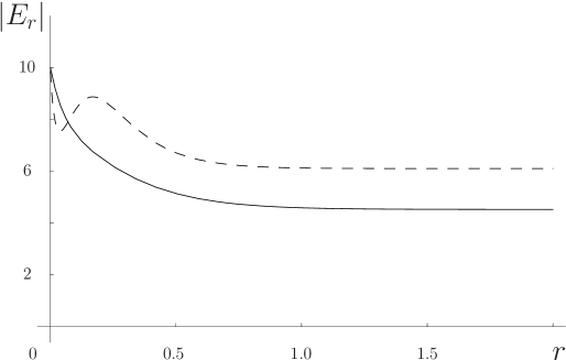
(b)

Figure 2: (a) $\tau(r)$. (b) $|E_{r}(r)|$. $n=1$ case for solid lines and $n=2$ case for dashed lines. We set $2{\cal T}_{p}=Q_{{\rm F}1}$ for numerical analysis.

Energy density $-T^{t}_{\;t}$ and radial pressure $T^{r}_{\;r}$ have the same functional forms with (2.11)–(2.12) by replacing $X$ in (2.20), but angular pressure is different;

$$T^{\theta}_{\;\theta}=-\frac{2{\cal T}_{p}V}{\sqrt{X}}\left(1+\tau^{\prime 2}-E_{r}^{2}\right).$$ (2.33)

$\theta$-component of the U(1) current is

$$j^{\theta}=\frac{2{\cal T}_{p}V}{\sqrt{X}}(1+\tau^{\prime 2}-E_{r}^{2})\frac{n}{r^{2}}\tau^{2},$$ (2.34)

and it satisfies conservation law $\nabla_{\mu}j^{\mu}=0$.

Near the origin we read behavior of densities, (2.11)–(2.12) and (2.33)–(2.34), by substituting (2.30)–(2.31)

$$T^{t}_{\;t} \approx -\sqrt{1+\tau_{0}^{2}}\,\frac{|Q_{{\rm F1}}|}{r}\left\{1+\frac{2{\cal T}_{p}^{2}}{Q_{\rm F1}^{2}}~{}[1+\tau_{0}^{2}(2n^{2}-1)]r^{2}+{\cal O}(r^{4})\right\},$$ (2.35)

$$T^{r}_{\;r} \approx -\frac{1}{\sqrt{1+\tau_{0}^{2}}}\,\frac{|Q_{{\rm F1}}|}{r}\left\{1+\frac{2{\cal T}_{p}^{2}}{Q_{\rm F1}^{2}}(1+\tau_{0}^{2})~{}r^{2}+{\cal O}(r^{4})\right\},$$ (2.36)

$$T^{\theta}_{\;\theta} \approx -4{\cal T}_{p}^{2}\sqrt{1+\tau_{0}^{2}}\,\frac{r}{|Q_{{\rm F1}}|}+{\cal O}(r^{3}),$$ (2.37)

$$j^{\theta} \approx 4{\cal T}_{p}^{2}\tau_{0}^{2}\sqrt{1+\tau_{0}^{2}}\,\frac{r}{|Q_{{\rm F1}}|}+{\cal O}(r^{3}).$$ (2.38)

The energy density (2.35) and radial pressure (2.36) are singular at the origin. Here the source of the singularity is identified with the singular fundamental string charge (2.32) at the origin so that contribution from the vortex configuration represented by the tachyon amplitude is regular. The singular behavior in this DBI type theory becomes milder (${\cal O}(1/r)$) in comparison with that in Maxwell theory in a plane ($E_{r}^{2}\sim 1/r^{2}$) so that self-energy of the fundamental string does not involve UV divergence.

From (2.28) and (2.29), the asymptotic forms of energy density and radial pressure show long-range term for sufficiently large $r$, but the angular pressure and the U(1) current do not as expected;

$$T^{t}_{\;t} \approx -\sqrt{1+\tau_{\infty}^{2}}\,~{}\frac{|Q_{{\rm F1}}|}{r}\left[1+\frac{16{\cal T}_{p}^{2}}{Q_{\rm F1}^{2}}(1+n^{2}\tau_{\infty}^{2})r^{2}e^{-2\frac{\tau_{\infty}r+\delta}{R}}+{\cal O}(re^{-2\frac{\tau_{\infty}r+\delta}{R}})\right],$$ (2.39)

$$T^{r}_{\;r} \approx -\frac{1}{\sqrt{1+\tau_{\infty}^{2}}}\,~{}\frac{|Q_{{\rm F1}}|}{r}\left\{1+\frac{8{\cal T}_{p}^{2}R}{\tau_{\infty}Q_{\rm F1}^{2}}\left[1+n^{2}\tau_{\infty}^{2}\left(1+\frac{2\delta}{R}\right)\right]re^{-2\frac{\tau_{\infty}r+\delta}{R}}\right.$$ (2.40)

$$\hskip 105.27519pt\left.+{\cal O}(e^{-2\frac{\tau_{\infty}r+\delta}{R}})\right\},$$

$$T^{\theta}_{\;\theta} \approx -16{\cal T}_{p}^{2}\frac{\sqrt{1+\tau_{\infty}^{2}}}{|Q_{\rm F1}|}re^{-2\frac{\tau_{\infty}r+\delta}{R}}\left[1+{\cal O}(1/r)\right],$$ (2.41)

$$j^{\theta} \approx 16{\cal T}_{p}^{2}n\frac{\tau_{\infty}^{2}\sqrt{1+\tau_{\infty}^{2}}}{|Q_{\rm F1}|}re^{-2\frac{\tau_{\infty}r+\delta}{R}}\left[1+{\cal O}(1/r)\right].$$ (2.42)

Therefore, energy of the obtained vortex configuration is linearly divergent

$$E=2\pi\int_{0}^{R_{{\rm IR}}}drrT_{tt}\propto Q_{{\rm F1}}R_{{\rm IR}}\stackrel{{\scriptstyle R_{{\rm IR}}\rightarrow\infty}}{{\longrightarrow}}\infty.$$ (2.43)

This linear divergence due to the fundamental string charge at the origin might be different from the familiar nature of logarithmically divergent energy of the global vortex.

Radial distribution of $-\sqrt{-g}\,T^{t}_{\;t}$ and $-\sqrt{-g}\,j^{\theta}$ are drawn in Fig. 3. From Fig. 3-(a) we can easily read the numerical values of $\tau_{0}$ under $2{\cal T}_{p}=Q_{{\rm F}1}$ and $\tau_{\infty}$, and the U(1) current is localized near the origin as shown in Fig. 3-(b).

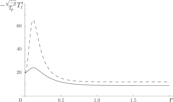
(a)

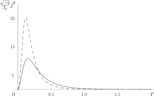
(b)

Figure 3: (a) $-\sqrt{-g}\,T^{t}_{\;t}/{\cal T}_{p}$. (b) $\sqrt{-g}\,j^{\theta}/{\cal T}_{p}$. $n=1$ case for solid lines and $n=2$ case for dashed lines.

Thin limit is achieved by taking the limit of infinite $\tau_{\infty}$. Then, from (2.29) and (2.39)–(2.42), $E_{r}$ and $-\sqrt{-g}\,T^{t}_{\;t}$ go to infinity but all the pressure components and the U(1) current vanish, which lets the limiting process of singular zero thickness with keeping constant $Q_{{\rm F}1}$ smooth.

3 Local D-Vortices

When the U(1)$\times$U(1) gauge fields in (1.1) are rewritten as $A_{\mu}=(A^{1}_{\mu}+A^{2}_{\mu})/2$ and $C_{\mu}=(A^{1}_{\mu}-A^{2}_{\mu})/2$, the former $A_{\mu}$ remains to be massless in symmetric phase and the latter $C_{\mu}$ becomes massive in broken phase. It is easily read by the form of the action

$$S=-{\cal T}_{p}\int d^{p+1}x\,V(T)\left[\,\sqrt{-\det(X^{+}_{\mu\nu})}+\sqrt{-\det(X^{-}_{\mu\nu})}\,\,\right],$$ (3.1)

where $C_{\mu\nu}=\partial_{\mu}C_{\nu}-\partial_{\nu}C_{\mu}$, $D_{\mu}T=(\partial_{\mu}-2iC_{\mu})T$, and

$$X^{\pm}_{\mu\nu}=g_{\mu\nu}+F_{\mu\nu}\pm C_{\mu\nu}+({\overline{D_{\mu}T}}D_{\nu}T+{\overline{D_{\nu}T}}D_{\mu}T)/2.$$ (3.2)

Note that the charge of $T$ is 2 in the unit system of consideration. In this coincidence limit, the D-brane is distinguished from the $\bar{{\rm D}}$-brane by coupling to the gauge field $C_{\mu}$.

For $F_{\mu\nu}$, we employ the same configuration, i.e., all the components vanish for singular local D-vortex and $F_{0r}$ is turned on for regular local D-vortex as has been done for global D-vortices.

3.1 Singular local D-vortex

In the subsection 2.1, we dealt with global D-vortices with vanishing $F_{\mu\nu}$. In this subsection we consider local D-vortices with vanishing $F_{\mu\nu}$ but with nonvanishing gauge field $C_{\mu}$. A minimal gauge field configuration for the local D-vortices superimposed at the origin is to turn only on the angular component $C_{\mu}=\delta_{\mu}^{\;\theta}C_{\theta}$ under the Weyl gauge $C_{0}=0$.

Substituting the ansatz (2.5) and the gauge field $C_{\theta}$ into the equations of motion, we obtain tachyon equation

$$\frac{1}{r}\frac{d}{dr}\left\{\frac{rV}{\sqrt{X}}\left[1+\frac{\tau^{2}}{r^{2}}(n-2C_{\theta})^{2}\right]~{}\tau^{\prime}\right\}-\frac{V}{\sqrt{X}}(1+\tau^{{}^{\prime}2})\tau\frac{(n-2C_{\theta})^{2}}{r^{2}}=\sqrt{X}~{}\frac{dV}{d\tau},$$ (3.3)

and equation of the gauge field

$$\frac{d}{dr}\left(\frac{rV}{\sqrt{X}}\frac{C_{\theta}^{{}^{\prime}}}{r^{2}}\right)+2\frac{rV}{\sqrt{X}}\left(1+\tau^{\prime 2}\right)\frac{\tau^{2}}{r^{2}}(n-2C_{\theta})=0,$$ (3.4)

where $C_{r\theta}=C_{\theta}^{{}^{\prime}}=dC_{\theta}/dr$ and

$$X\equiv\left(1+\tau^{{}^{\prime}2}\right)\left[1+(n-2C_{\theta})^{2}\frac{\tau^{2}}{r^{2}}\right]+\frac{C_{\theta}^{{}^{\prime}2}}{r^{2}}.$$ (3.5)

Since we look for nonsingular solutions of the equations of motion, (3.3) and (3.4), the ansatz (2.5) is used for the tachyon field and the form of gauge field, $C_{i}=-\epsilon_{ij}x^{j}C_{\theta}(r)/r^{2}$ ($\epsilon_{12}=1$), forces the following boundary condition at the origin as

$$C_{\theta}(r=0)=0.$$ (3.6)

In addition to the boundary condition of the tachyon field at infinity (2.8), value of the gauge field $C_{\theta}$ at infinity should be

$$C_{\theta}(r=\infty)=n/2$$ (3.7)

to make the $(n-2C_{\theta})$-term in the energy density, radial pressure, and $\theta$-component of U(1) current vanish at infinity;

$$T^{t}_{\;t} = -\frac{2{\cal T}_{p}V}{\sqrt{X}}\left\{\left(1+\tau^{\prime 2}\right)\left[1+(n-2C_{\theta})^{2}\frac{\tau^{2}}{r^{2}}\right]+\frac{C_{\theta}^{{}^{\prime}2}}{r^{2}}\right\},$$ (3.8)

$$T^{r}_{\;r} = -\frac{2{\cal T}_{p}V}{\sqrt{X}}\left[1+(n-2C_{\theta})^{2}\frac{\tau^{2}}{r^{2}}\right],$$ (3.9)

$$j^{\theta} = \frac{2{\cal T}_{p}V}{\sqrt{X}}(1+\tau^{\prime 2})\frac{\tau^{2}}{r^{2}}(n-2C_{\theta}).$$ (3.10)

Another nonvanishing component of energy-momentum tensor is

$$T^{\theta}_{\;\theta} = -\frac{2{\cal T}_{p}V}{\sqrt{X}}\left(1+\tau^{\prime 2}\right).$$ (3.11)

If we try $C_{\theta}(r)\approx C_{\infty}r^{q}$ to the equation of gauge field, its left-hand side of (3.4) vanishes only when (3.7) is satisfied.

Substituting the boundary conditions at infinity, (2.8) and (3.7), into the tachyon equation, (3.3) reduces approximately to the tachyon equation with zero vorticity $(n=0)$ and gauge field $(C_{\theta}=0)$:

$$\tau^{\prime\prime}+\left(\frac{1}{r}-\frac{\tau^{\prime}}{R}-\frac{1}{2}\frac{X^{\prime}}{X}\right)\tau^{\prime}\approx-\frac{1+\tau^{{}^{\prime}2}}{R}.$$ (3.12)

For the tachyon $\tau(r)\approx\tau_{\infty}r^{k},~{}(k\geq 0)$ at asymptotic region, the left-hand side cannot be equated with the right-hand side. Therefore, nonexistence of static regular local D-vortex solutions satisfying (2.8) and (3.7) is obvious. It means that the static singular local D-vortex configuration in Ref. [15] cannot be understood as a singular limit of static regular local D-vortex solution.

We showed nonexistence of the regular static local vortices satisfying the boundary conditions, (2.7)–(2.8) and (3.6)–(3.7), however it has been known to exist the singular local vortices satisfying the same boundary conditions in Ref. [15]. Let us reconfirm the existence of such solution relying on the information of boundary string field theory in what follows [13].

Suppose that the vortex configuration of vorticity $n$ is given by $\tau\sim r/\epsilon$ as has been studied in boundary string field theory [13] and in the subsection 2.1. For the gauge field we set $C_{\theta}=(n/2)[1-f(r)]$, where $f(r)$ should satisfy $f(0)=1$ and $f(\infty)=0$ according to the boundary conditions (3.6) and (3.7). Substituting these into (3.5), we have

$$X=\left(1+\frac{1}{\epsilon^{2}}\right)\left(1+\frac{n^{2}}{\epsilon^{2}}f^{2}\right)+\frac{n^{2}}{4r^{2}}f^{\prime 2}.$$ (3.13)

Now let us assume that $\epsilon$ is sufficiently small. Since $f(r)$ is a monotonic decreasing function, $f$ has almost unity for $r<\epsilon R$ and zero for $r>\epsilon R$. In the expression of $X$ (3.13), possible candidates of the leading term would be $1/\epsilon^{2}$, $n^{2}f^{2}/\epsilon^{4}$, and $n^{2}f^{\prime 2}/4r^{2}$. Near $r\approx 0$, $n^{2}f^{2}/\epsilon^{4}$ or $n^{2}f^{\prime 2}/4r^{2}$ is dominant so that (3.4) supports a solution $f\sim e^{-\frac{4R}{3\epsilon^{3}}r^{3}}$. For large $r$, $1/\epsilon^{2}$-term is dominant so that the approximated equation of (3.4) leads to $f(r)\approx ce^{-r^{2}/\epsilon^{2}}$. When $\epsilon\rightarrow 0$, the energy density has $\delta$-function like singularity at the origin, $-T^{t}_{\;t}(0)\approx 2{\cal T}_{p}n/\epsilon^{2}\stackrel{{\scriptstyle\epsilon\rightarrow 0}}{{\longrightarrow\infty}}$, but the pressures remain constant, $T^{r}_{\;r}(0)\approx-2{\cal T}_{p}n$ and $T^{\theta}_{\;\theta}(0)\approx-2{\cal T}_{p}/n$. At $r\neq 0$, $-T^{t}_{\;t}=T^{r}_{\;r}=T^{\theta}_{\;\theta}=0$ for $n=1$. Therefore, the conservation law equivalent to the tachyon equation is satisfied in the $\epsilon\rightarrow 0$ limit, i.e., $(T^{r}_{\;r})^{\prime}=-(T^{r}_{\;r}-T^{\theta}_{\;\theta})/r=0$.

Tension of the singular D$0$-brane with vanishing thickness is

$$2{\cal T}_{0}^{\ell} = \int_{0}^{\infty}d\theta\int_{0}^{\infty}drr(-T^{t}_{t})$$ (3.14)

$$\approx 4\pi R^{2}{\cal T}_{2}\int_{0}^{\infty}dy\frac{\sqrt{1+16y^{2}}e^{-16y^{3}/3}}{\cosh y},$$

$$= 2(\sqrt{2\times 0.26254\times\pi}R)^{2}{\cal T}_{2},$$ (3.15)

where $y=r/\epsilon R$ and $R=\sqrt{2}$. If we compare the obtained tension of local singular D-vortex (3.15) with that of global singular D-vortex (2.17), the energy of singular D-vortex is significantly lowered by the gauge field $C_{\theta}$, i.e., ${\cal T}_{0}^{\ell}/{\cal T}_{0}^{g}$ is about 0.14. Due to the gauge field, the D$0$-brane also carries the quantized magnetic flux

$$\Phi = \int_{0}^{\infty}dr\int_{0}^{2\pi}d\theta\,C_{r\theta}$$ (3.16)

$$= 2\pi\left[C_{\theta}(r=\infty)-C_{\theta}(r=0)\right]$$

$$= \pi n.$$ (3.17)

3.2 Regular local D-vortex with electric flux

Let us turn on $F_{0r}=E_{r}$ again. Then the effective action (3.1) becomes

$$\frac{S}{\int d^{p-2}x_{\perp}}=-2{\cal T}_{p}\int dtdrd\theta rV(\tau)\sqrt{X}\,,$$ (3.18)

where

$$X\equiv\left(1+\tau^{{}^{\prime}2}-E_{r}^{2}\right)\left[1+(n-2C_{\theta})^{2}\frac{\tau^{2}}{r^{2}}\right]+\frac{C_{\theta}^{{}^{\prime}2}}{r^{2}}.$$ (3.19)

We read tachyon equation

$$\frac{1}{r}\frac{d}{dr}\left\{\frac{rV}{\sqrt{X}}\left[1+\frac{\tau^{2}}{r^{2}}(n-2C_{\theta})^{2}\right]~{}\tau^{\prime}\right\}-\frac{V}{\sqrt{X}}(1+\tau^{{}^{\prime}2}-E_{r}^{2})\tau\frac{(n-2C_{\theta})^{2}}{r^{2}}=\sqrt{X}~{}\frac{dV}{d\tau}.$$ (3.20)

Equation for the gauge field $A_{\mu}$ is obtained from constancy of the conjugate momentum $\Pi^{r}$ multiplied by $r$ (2.22). Specific form of the conjugate momentum $\Pi^{r}$ is

$$\Pi^{r}\equiv\frac{1}{\sqrt{-g}}\frac{\delta S}{\delta(\partial_{t}A_{r})}=\frac{1}{\sqrt{-g}}\frac{\delta S}{\delta F_{tr}}=\frac{2{\cal T}_{p}V}{\sqrt{X}}\left[1+(n-2C_{\theta})^{2}\frac{\tau^{2}}{r^{2}}\right]E_{r}(r),$$ (3.21)

and thereby the electric field is

$$E_{r}^{2}(r)=\frac{(1+\tau^{\prime 2})\left[1+(n-2C_{\theta})^{2}\frac{\tau^{2}}{r^{2}}\right]+\frac{C_{\theta}^{{}^{\prime}2}}{r^{2}}}{\left[1+(n-2C_{\theta})^{2}\frac{\tau^{2}}{r^{2}}\right]\left\{1+\left(\frac{2{\cal T}_{p}V}{\Pi^{r}}\right)^{2}\left[1+(n-2C_{\theta})^{2}\frac{\tau^{2}}{r^{2}}\right]\right\}}.$$ (3.22)

Nonvanishing field strength of the gauge field $C_{\mu}$ is $C_{r\theta}=C_{\theta}^{{}^{\prime}}(r)$ which automatically satisfies Bianchi identity, $\partial_{\mu}C_{\nu\rho}+\partial_{\nu}C_{\rho\mu}+\partial_{\rho}C_{\mu\nu}=0$. Equation of the gauge field $C_{\mu}$ is

$$\frac{1}{r}\frac{d}{dr}\left(\frac{rV}{\sqrt{X}}\frac{C_{\theta}^{{}^{\prime}}}{r^{2}}\right)+2\frac{V}{\sqrt{X}}\left(1+\tau^{\prime 2}-E_{r}^{2}\right)\tau^{2}\frac{n-2C_{\theta}}{r^{2}}=0.$$ (3.23)

Regarding the boundary condition of radial component of electric field $E_{r}$ at infinity, vanishing $\theta$-component of pressure

$$T^{\theta}_{\;\theta} = -\frac{2{\cal T}_{p}V}{\sqrt{X}}\left(1+\tau^{\prime 2}-E_{r}^{2}\right)$$ (3.24)

requires

$$E_{r}^{2}(\infty)\rightarrow 1+\tau^{{}^{\prime}2}(\infty).$$ (3.25)

Then the $\theta$-component of U(1) current

$$j^{\theta}=\frac{2{\cal T}_{p}V}{\sqrt{X}}\left(1+\tau^{\prime 2}-E_{r}^{2}\right)\frac{\tau^{2}}{r^{2}}(n-2C_{\theta})$$ (3.26)

also decays to zero rapidly as $r$ increases. Note that the energy density $-T^{t}_{\;t}$ and the radial pressure $T^{r}_{\;r}$ with nonvanishing $E_{r}$ share the same functional forms with $T^{t}_{\;t}$ (3.8) and $T^{r}_{\;r}$ (3.9) without $E_{r}$ except for the difference in the expression of determinant $X$ (3.19).

The D-vortices of interest are characterized by the fundamental string charge $Q_{{\rm F1}}$ with density $\Pi^{r}$ (3.21) and the topological charge represented by the magnetic flux (3.17). In the last line (3.17), we used the boundary condition (3.7), and the result (3.17) means that unit of the magnetic flux is $\pi$ where the denominator 2 in $2\pi n/2$ comes from the charge of complex tachyon field.

Power series expansion near the origin shows that the tachyon $\tau$ and the gauge field $C_{\theta}$ are increasing but radial electric field $E_{r}$ decreases due to negative $\gamma$;

$$\tau(r) \approx \tau_{0}r[1+\alpha r^{2}+{\cal O}(r^{4})],$$ (3.27)

$$C_{\theta}(r) \approx C_{0}r^{3}[1+\beta r^{2}+{\cal O}(r^{3})],$$ (3.28)

$$E_{r}^{2}(r) \approx (1+\tau_{0}^{2})[1+\gamma r^{2}+{\cal O}(r^{4})],$$ (3.29)

where

$$\alpha=-\frac{n^{2}-1}{6(1+\tau_{0}^{2}n^{2})}\left[9C_{0}^{2}-\frac{4{\cal T}_{p}^{2}}{Q_{\rm F1}^{2}}(1+\tau_{0}^{2})(1+\tau_{0}^{2}n^{2})^{2}\right],$$ (3.30)

$$\beta=\frac{3+\tau_{0}^{2}n^{2}(5-2n^{2})}{10(1+\tau_{0}^{2}n^{2})^{3}}\left[9C_{0}^{2}-\frac{4{\cal T}_{p}^{2}}{Q_{\rm F1}^{2}}(1+\tau_{0}^{2})(1+\tau_{0}^{2}n^{2})^{2}\right],$$ (3.31)

$$\gamma=\frac{1}{(1+\tau_{0}^{2}n^{2})^{2}}\left[9C_{0}^{2}-\frac{4{\cal T}_{p}^{2}}{Q_{\rm F1}^{2}}(1+\tau_{0}^{2})(1+\tau_{0}^{2}n^{2})^{2}\right].$$ (3.32)

For sufficiently large $r$, functional forms of the tachyon amplitude and electric field rapidly approach asymptotic configurations

$$\tau(r) \sim \tau_{\infty}r+\delta-4\frac{{\cal T}_{p}^{2}R(1+\tau_{\infty}^{2})}{\tau_{\infty}^{2}Q_{\rm F1}^{2}}~{}r^{2}e^{-2\frac{\tau_{\infty}r+\delta}{R}}+{\cal O}(re^{-2\frac{\tau_{\infty}r+\delta}{R}}),$$ (3.33)

$$E_{r}^{2}(r) \sim (1+\tau_{\infty}^{2})\left[1-16\frac{{\cal T}_{p}^{2}R}{\tau_{\infty}Q_{\rm F1}^{2}}re^{-2\frac{\tau_{\infty}r+\delta}{R}}+{\cal O}(r^{4}e^{-4\frac{\tau_{\infty}r+\delta}{R}})\right],$$ (3.34)

where $\tau_{\infty}$ and $\delta$ are constants which cannot be determined only by the boundary conditions at infinity. For the gauge field $C_{\theta}$, let us try

$$C_{\theta}(r)\sim\frac{n}{2}+\delta C_{\theta},$$ (3.35)

then the linearized equation of $\delta C_{\theta}$ from (3.23) reduces to

$$M(t)\frac{d^{2}\delta C_{\theta}}{dt^{2}}=-\frac{d}{d\delta C_{\theta}}U(\delta C_{\theta}),\qquad t=\kappa r^{3},~{}\left(\kappa=\frac{4{\cal T}_{p}\tau_{\infty}}{3|Q_{\rm F1}|}\sqrt{1+\tau_{\infty}^{2}}e^{-\frac{\delta}{R}}\right)$$ (3.36)

which describes the one-dimensional motion of a hypothetical point particle with exponentially-increasing “time-dependent mass” $M(t)=e^{2\tau_{\infty}t^{1/3}/(R\kappa^{1/3})}$. Since the force is given by a conservative potential $U=-(\delta C_{\theta})^{2}/2$, possible boundary values of $\delta C_{\theta}$ at infinity are read as $\delta C_{\theta}(\infty)=\pm\infty~{}(\mbox{minima})$ or $\delta C_{\theta}(\infty)=0~{}(\mbox{maximum})$. Though we do not obtain the solution satisfying $\delta C_{\theta}(\infty)=0$ $(C_{\theta}(\infty)=n/2)$ analytically, existence of such solution is obvious. The boundary condition at the origin (3.6) and the shape of $U(\delta C_{\theta})$ require that $\delta C_{\theta}$ is negative and monotonic increasing to zero.

The obtained numerical results in Fig. 4 confirm the approximations at both the origin and infinity discussed previously. From Fig. 4-(a) and (c), the numerical value of $\tau_{\infty}$ is read to be 4.217 under $2{\cal T}_{p}/Q_{{\rm F}1}=1.2$.

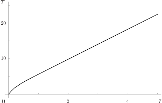
(a)

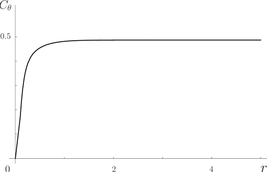
(b)

(c)

Figure 4: (a) $\tau(r)$. (b) $C_{\theta}(r)$. (c) $|E_{r}(r)|$. $n=1$ and $2{\cal T}_{p}/Q_{{\rm F}1}=1.2$.

If (3.27)–(3.28) are inserted in the energy-momentum tensor, (3.8)–(3.9), (3.24), and the current density (3.26), then profiles near the origin are

$$T^{t}_{\;t} \approx -\sqrt{1+\tau_{0}^{2}}~{}\frac{|Q_{\rm F1}|}{r}\left\{1+\frac{r^{2}}{2(1+\tau_{0}^{2}n^{2})^{2}}\left[9C_{0}^{2}+\frac{4{\cal T}_{p}^{2}}{Q_{\rm F1}^{2}}(1+\tau_{0}^{2}(2n^{2}-1))(1+\tau_{0}^{2}n^{2})^{2}\right]\right.$$ (3.37)

$$\hskip 99.58464pt\left.+{\cal O}(r^{4})\right\},$$

$$T^{r}_{\;r} \approx -\frac{1}{\sqrt{1+\tau_{0}^{2}}}~{}\frac{|Q_{\rm F1}|}{r}\left\{1-\frac{r^{2}}{2(1+\tau_{0}^{2}n^{2})^{2}}\left[9C_{0}^{2}-\frac{4{\cal T}_{p}^{2}}{Q_{\rm F1}^{2}}(1+\tau_{0}^{2})(1+\tau_{0}^{2}n^{2})^{2}\right]\right.$$ (3.38)

$$\hskip 99.58464pt\left.+{\cal O}(r^{4})\right\},$$

$$T^{\theta}_{\;\theta} \approx \frac{|Q_{\rm F1}|r}{(1+\tau_{0}^{2}n^{2})^{2}\sqrt{1+\tau_{0}^{2}}}\left[9C_{0}^{2}-\frac{4{\cal T}_{p}^{2}}{Q_{\rm F1}^{2}}(1+\tau_{0}^{2})(1+\tau_{0}^{2}n^{2})^{2}\right]+{\cal O}(r^{3}),$$ (3.39)

$$j^{\theta} \approx -\frac{\tau_{0}^{2}n|Q_{\rm F1}|r}{(1+\tau_{0}^{2}n^{2})^{2}\sqrt{1+\tau_{0}^{2}}}\left[9C_{0}^{2}-\frac{4{\cal T}_{p}^{2}}{Q_{\rm F1}^{2}}(1+\tau_{0}^{2})(1+\tau_{0}^{2}n^{2})^{2}\right]+{\cal O}(r^{3}).$$ (3.40)

Substituting (3.33)–(3.35) into (3.8) (3.9) (3.24) (3.26), we notice that, as in the case of global DF-vortices, the energy density and the radial component of pressure have a long range term but the $\theta$-components of pressure and U(1) current do not;

$$T^{t}_{\;t} \sim -\sqrt{1+\tau_{\infty}^{2}}~{}\frac{|Q_{\rm F1}|}{r}\left[1+\frac{16{\cal T}_{p}^{2}}{Q_{\rm F1}^{2}}~{}r^{2}e^{-2\frac{\tau_{\infty}r+\delta}{R}}+{\cal O}(re^{-2\frac{\tau_{\infty}r+\delta}{R}})\right],$$ (3.41)

$$T^{r}_{\;r} \sim -\frac{1}{\sqrt{1+\tau_{\infty}^{2}}}~{}\frac{|Q_{\rm F1}|}{r}\left[1+\frac{8{\cal T}_{p}^{2}R}{\tau_{\infty}Q_{\rm F1}^{2}}re^{-2\frac{\tau_{\infty}r+\delta}{R}}+{\cal O}(r^{4}e^{-4\frac{\tau_{\infty}r+\delta}{R}})\right],$$ (3.42)

$$T^{\theta}_{\;\theta} \sim -16\frac{{\cal T}_{p}^{2}\sqrt{1+\tau_{\infty}^{2}}}{|Q_{\rm F1}|}~{}re^{-2\frac{\tau_{\infty}r+\delta}{R}}\left[1+{\cal O}(re^{-2\frac{\tau_{\infty}r+\delta}{R}})\right],$$ (3.43)

$$j^{\theta} \sim -32{\cal T}_{p}^{2}\frac{\tau_{\infty}^{2}\sqrt{1+\tau_{\infty}^{2}}}{|Q_{\rm F1}|}re^{-2\frac{\tau_{\infty}r+\delta}{R}}\delta C_{\theta}.$$ (3.44)

Note that the coefficients of the leading terms of $T^{t}_{\;t}$ (3.41) and $T^{r}_{\;r}$ (3.42) coincide exactly with those in (2.39) and (2.40) except for the value of $\tau_{\infty}$, which means that the leading behavior at asymptotic region is governed by the fundamental strings. The effect of the gauge field $C_{\theta}$ appears in the subleading term, which makes the fields approach their boundary behaviors at infinity more rapidly. Fig. 5-(a),(b) show that the localized parts near the origin have the ring shape. Since the leading term of the energy density decreases with $1/r$, we can read the value of $\tau_{\infty}=4.217$ again from the Fig. 5-(a), which is exactly the same as that from the figure of $\tau(r)$ in Fig. 2-(a).

(a)

(b)

Figure 5: (a) $-\sqrt{-g}\,T^{t}_{\;t}/{\cal T}_{p}$. (b) $\sqrt{-g}\,j^{\theta}/{\cal T}_{p}$.

Though we obtained the regular solutions in subsections 2.2 and 3.2, the stability of D-vortices and D-strings with electric flux should be studied including production of closed string degrees of freedom [16] as has been discussed in Ref. [8].

4 From D-vortices to D-strings

For unstable D-branes, the coupling to the bulk RR fields can be read off from the Wess-Zumino term [13, 14, 15, 30] and, for D$p{\bar{\rm D}}p$, it is possibly be extended as

$$S_{\rm WZ} = \mu~{}{\rm Str}\int_{\Sigma_{3}}C_{\rm RR}\wedge{\rm exp}\left(\begin{array}[]{cc}F^{1}-T\bar{T}&i^{3/2}~{}DT\\ -i^{3/2}~{}\overline{DT}&F^{2}-\bar{T}T\end{array}\right)$$

$$= \mu\int_{\Sigma_{3}}e^{-T\bar{T}}C_{\rm RR}\wedge(2C+iDT\wedge\overline{DT})$$

$$= 2\mu\int_{\Sigma_{3}}C_{\rm RR}\wedge dr\wedge d\theta~{}\frac{d}{dr}\left[e^{-\tau^{2}}\left(C_{\theta}-\frac{n}{2}\right)\right],$$ (4.4)

where $\mu$ is a real constant and the supertrace ${\rm Str}$ is defined to be a trace with insertion of $\sigma_{3}$. Note that $C\equiv C_{\mu\nu}dx^{\mu}\wedge dx^{\nu}$ and $C_{\mu\nu}=(F^{1}_{\mu\nu}-F^{2}_{\mu\nu})/2$. For the D2${\bar{\rm D}}$2 system, it is obvious that all the singular and regular, global ($C_{\theta}=0$) and local D-vortices on the D2${\bar{\rm D}}$2 carry only D0 charge. In addition, the total D0 charge ($=4\pi\mu\int dr\frac{d}{dr}[e^{-\tau^{2}}\left(C_{\theta}-\frac{n}{2}\right)]=2\pi\mu n$) is exactly proportional to the vorticity $n$ (or the quantized magnetic flux (3.17) for the local vortex) irrespective of the nature of the D-vortices, global or local, as expected.

An extension from D-vortices to straight D-strings is straightforwardly made by considering the coincidence limit of D3${\bar{\rm D}}$3-system (with fundamental strings) instead of the D2${\bar{\rm D}}$2. Since our analysis is based on the DBI-type effective field theory action (1.1), the matrices $X_{\mu\nu}$ (2.2) and $X_{\mu\nu}^{\pm}$ (3.2) inside the actions (2.1) and (3.1) become $4\times 4$-matrices with coordinate $(t,r,\theta,z)$ instead of $3\times 3$ matrices. For straight D-strings stretched along the $z$-direction, additional components of the matrices can be assumed to have $X_{tz}=X_{tz}^{\pm}=0$ and $X_{zz}=X_{zz}^{\pm}=1$ so that $S/\int dz$ is the same as the actions (2.1) and (3.1) due to translational symmetry along the $z$-direction. Then the one-dimensional RR-charge is derived, and the stringy objects are identified with singular and regular D1-branes (D-strings).

In this paper we obtained singular and regular D-strings (D1-branes) given by global and local vortex-string solutions. Another attractive stringy configuration is DF-string or $(p,q)$-string (composite of D1F1), which also plays an important role as a cosmic string [5]. In the scheme of effective field theory, the simplest straight DF-string can be achieved by adding another component of Born-Infeld type U(1) gauge field, i.e., it is localized $E_{z}(r)=F_{tz}(r)$. If we find a string solution with the RR-charge and the fundamental string charge density $\Pi_{z}$ confined along the string, the obtained stringy objects must be straight DF-string.

If we turn on angular component of the electric field $E_{\theta}=F_{0\theta}$, the classical equations of motion force it to be constant and are not likely to support such static vortex solutions. In terms of string theory, this impossibility seems natural since existence of such constant $E_{\theta}$ implies distribution of closed strings melted on the D-brane to infinity with constant density.

In curved spacetime the obtained D-strings become candidates of cosmic superstrings, i.e., they are straight cosmic D-strings. The spacetime structure formed by these D-strings is of interest in cosmology, and the first specific question is emergence of conical space at asymptotic region when the cosmological constant vanishes. Cosmic D-strings are mostly generated after the brane and antibrane meet, which means post inflationary era since the inflation on brane-antibrane occurs before the brane and antibrane meet.

5 Conclusion

In this paper we considered DBI-type effective action of a complex tachyon and gauge fields of U(1)$\times$U(1) symmetry, describing brane-antibrane system with fundamental strings. In the coincidence limit of D2${\bar{\rm D}}$2, static vortex solutions are obtained. Without DBI electromagnetic field, there exist only singular static global and local D-vortex solutions. When the radial component of electric field is turned on, we found regular static global and local D-vortex solutions. The obtained point-like D-vortex configurations are naturally embedded in straight stringy solutions in D3${\bar{\rm D}}$3-system, and are identified with D-strings (D1-branes). If the obtained macroscopic D-strings are gravitating, they become naturally candidates of cosmic D-strings in the early Universe.

We conclude the paper with a few discussions for further study. First, we only considered D${\bar{\rm D}}$ in the coincidence limit through this paper, however it is intriguing to take into account the effect coming from separation of D and ${\bar{\rm D}}$. In the effective field theory, it means inclusion of the transverse coordinates and dynamics of cosmological time evolution, e.g., inflation. Second, in the superstring theory setting, the worldvolume of D3${\bar{\rm D}}3$-system comprises a noncompact (1+3)-dimensional bulk in ten dimensions. The remaining six-dimensions are assumed to be compactified and their size effect was completely neglected in this work. Since the tension of D-branes is naturally in string scale, a consistent approach including KK-modes makes our analysis more concrete. Third, Nielsen-Olesen vortices of Abelian-Higgs model are scattered to 90 degrees and this property leads to intercommutation (reconnection) of two colliding cosmic strings. But, according to Ref. [5, 9], colliding DF-strings may result in a connected tree structure composed of a pair of trilinear vertices and it can finally form a cosmic DF-string network. This issue was dealt in the context of Yang-Mills theory [31] but it needs further study by using the obtained D(F)-strings and the DBI-type nonlocal effective action.

References

- [1] A. Vilenkin and E. P. S. Shellard, Cosmic Strings and Other Topological Defects, (Cambridge University Press, 1984).
- [2] T. W. B. Kibble, “Cosmic strings reborn?,” arXiv:astro-ph/0410073.
- [3] E. Witten, “Cosmic Superstrings,” Phys. Lett. B 153, 243 (1985).
- [4] G. Dvali and A. Vilenkin, “Formation and evolution of cosmic D-strings,” JCAP 0403, 010 (2004) [arXiv:hep-th/0312007].
- [5] E. J. Copeland, R. C. Myers and J. Polchinski, “Cosmic F- and D-strings,” JHEP 0406, 013 (2004) [arXiv:hep-th/0312067].
- [6] For a review, see J. Polchinski, “Introduction to cosmic F- and D-strings,” arXiv:hep-th/0412244.
- [7] E. Halyo, “Cosmic D-term strings as wrapped D3 branes,” JHEP 0403, 047 (2004) [arXiv:hep-th/0312268]; J. Urrestilla, A. Achucarro and A. C. Davis, “D-term inflation without cosmic strings,” Phys. Rev. Lett. 92, 251302 (2004) [arXiv:hep-th/0402032]; T. Matsuda, “String production after angled brane inflation,” Phys. Rev. D 70, 023502 (2004) [arXiv:hep-ph/0403092]; K. Dasgupta, J. P. Hsu, R. Kallosh, A. Linde and M. Zagermann, “D3/D7 brane inflation and semilocal strings,” JHEP 0408, 030 (2004) [arXiv:hep-th/0405247]; A. Achucarro and J. Urrestilla, “F-term strings in the Bogomolnyi limit are also BPS states,” JHEP 0408, 050 (2004) [arXiv:hep-th/0407193]; T. Damour and A. Vilenkin, “Gravitational radiation from cosmic (super)strings: Bursts, stochastic background, and observational windows,” Phys. Rev. D 71, 063510 (2005) [arXiv:hep-th/0410222]; N. Barnaby, A. Berndsen, J. M. Cline and H. Stoica, “Overproduction of cosmic superstrings,” JHEP 0506, 075 (2005) [arXiv:hep-th/0412095]; H. Firouzjahi and S. H. Tye, “Brane inflation and cosmic string tension in superstring theory,” JCAP 0503, 009 (2005) [arXiv:hep-th/0501099]; S. C. Davis, P. Binetruy and A. C. Davis, “Local axion cosmic strings from superstrings,” Phys. Lett. B 611, 39 (2005) [arXiv:hep-th/0501200]; S. H. Tye, I. Wasserman and M. Wyman, “Scaling of multi-tension cosmic superstring networks,” Phys. Rev. D 71, 103508 (2005) [Erratum-ibid. D 71, 129906 (2005)] [arXiv:astro-ph/0503506]; E. J. Copeland and P. M. Saffin, “On the evolution of cosmic-superstring networks,” arXiv:hep-th/0505110; J. J. Blanco-Pillado, G. Dvali and M. Redi, “Cosmic D-strings as axionic D-term strings,” arXiv:hep-th/0505172; A. C. Davis and K. Dimopoulos, “Cosmic superstrings and primordial magnetogenesis,” arXiv:hep-ph/0505242; P. M. Saffin, “A practical model for cosmic (p,q) superstrings,” arXiv:hep-th/0506138; H. Firouzjahi and S. H. Tye, “The tension spectrum of cosmic superstrings in a warped deformed conifold,” arXiv:hep-th/0506264; E. I. Buchbinder, “On Open Membranes, Cosmic Strings and Moduli Stabilization,” arXiv:hep-th/0507164.
- [8] L. Leblond and S. H. H. Tye, “Stability of D1-strings inside a D3-brane,” JHEP 0403, 055 (2004) [arXiv:hep-th/0402072].
- [9] M. G. Jackson, N. T. Jones and J. Polchinski, “Collisions of cosmic F- and D-strings,” arXiv:hep-th/0405229;
- [10] N. Jones, H. Stoica and S. H. H. Tye, “Brane interaction as the origin of inflation,” JHEP 0207, 051 (2002) [arXiv:hep-th/0203163].
- [11] G. Dvali, R. Kallosh and A. Van Proeyen, “D-term strings,” JHEP 0401, 035 (2004) [arXiv:hep-th/0312005].
- [12] S. Sarangi and S. H. H. Tye, “Cosmic string production towards the end of brane inflation,” Phys. Lett. B 536, 185 (2002) [arXiv:hep-th/0204074].
- [13] P. Kraus and F. Larsen, “Boundary string field theory of the DD-bar system,” Phys. Rev. D 63, 106004 (2001) [arXiv:hep-th/0012198]; T. Takayanagi, S. Terashima and T. Uesugi, “Brane-antibrane action from boundary string field theory,” JHEP 0103, 019 (2001) [arXiv:hep-th/0012210].
- [14] N. T. Jones and S. H. H. Tye, “An improved brane anti-brane action from boundary superstring field theory and multi-vortex solutions,” JHEP 0301, 012 (2003) [arXiv:hep-th/0211180].
- [15] A. Sen, “Dirac-Born-Infeld action on the tachyon kink and vortex,” Phys. Rev. D 68, 066008 (2003) [arXiv:hep-th/0303057].
- [16] N. Lambert, H. Liu and J. Maldacena, “Closed strings from decaying D-branes,” arXiv:hep-th/0303139.
- [17] C. Kim, Y. Kim and C. O. Lee, “Tachyon kinks,” JHEP 0305, 020 (2003) [arXiv:hep-th/0304180].
- [18] P. Brax, J. Mourad and D. A. Steer, “Tachyon kinks on non BPS D-branes,” Phys. Lett. B 575, 115 (2003) [arXiv:hep-th/0304197].
- [19] C. Kim, Y. Kim, O. K. Kwon and C. O. Lee, “Tachyon kinks on unstable Dp-branes,” JHEP 0311, 034 (2003) [arXiv:hep-th/0305092].
- [20] K. Hashimoto and S. Nagaoka, Phys. Rev. D 66, 026001 (2002) [arXiv:hep-th/0202079].
- [21] C. G. . Callan and J. M. Maldacena, “D-brane Approach to Black Hole Quantum Mechanics,” Nucl. Phys. B 472, 591 (1996) [arXiv:hep-th/9602043]; G. W. Gibbons, “Born-Infeld particles and Dirichlet p-branes,” Nucl. Phys. B 514, 603 (1998) [arXiv:hep-th/9709027].
- [22] A. Sen “Non-BPS states and branes in string theory,” arXiv:hep-th/9904207.
- [23] A. Sen, “Universality of the tachyon potential,” JHEP 9912, 027 (1999) [arXiv:hep-th/9911116].
- [24] D. Kutasov and V. Niarchos, “Tachyon effective actions in open string theory,” Nucl. Phys. B 666, 56 (2003) [arXiv:hep-th/0304045].
- [25] A. Buchel, P. Langfelder and J. Walcher, “Does the tachyon matter?,” Annals Phys. 302, 78 (2002) [arXiv:hep-th/0207235]; C. Kim, H. B. Kim, Y. Kim and O-K. Kwon, “Electromagnetic string fluid in rolling tachyon,” JHEP 0303, 008 (2003) [arXiv:hep-th/0301076]; F. Leblond and A. W. Peet, “SD-brane gravity fields and rolling tachyons,” JHEP 0304, 048 (2003) [arXiv:hep-th/0303035].
- [26] A. Sen, “Field theory of tachyon matter,” Mod. Phys. Lett. A 17, 1797 (2002) [arXiv:hep-th/0204143].
- [27] I. Cho and A. Vilenkin, “Vacuum defects without a vacuum,” Phys. Rev. D 59, 021701 (1999) [arXiv:hep-th/9808090]; I. Cho and A. Vilenkin, “Gravitational field of vacuumless defects,” Phys. Rev. D 59, 063510 (1999) [arXiv:gr-qc/9810049].
- [28] C. Kim, Y. Kim, O-K. Kwon and P. Yi, “Tachyon tube and supertube,” JHEP 0309, 042 (2003) [arXiv:hep-th/0307184].
- [29] C. Kim, Y. Kim and O. K. Kwon, “Tubular D-branes in Salam-Sezgin model,” JHEP 0405, 020 (2004) [arXiv:hep-th/0404163].
- [30] C. Kennedy and A. Wilkins, “Ramond-Ramond couplings on brane-antibrane systems,” Phys. Lett. B 464, 206 (1999) [arXiv:hep-th/9905195]; K. Okuyama, “Wess-Zumino term in tachyon effective action,” JHEP 0305, 005 (2003) [arXiv:hep-th/0304108].
- [31] K. Hashimoto and W. Taylor, “Strings between branes,” JHEP 0310, 040 (2003) [arXiv:hep-th/0307297]; A. Hanany and K. Hashimoto, “Reconnection of colliding cosmic strings,” arXiv:hep-th/0501031.