Solitons in Supersymmetric Gauge Theories
Abstract
Recent results on BPS solitons in the Higgs phase of supersymmetric (SUSY) gauge theories with eight supercharges are reviewed. For gauge theories with the hypermultiplets in the fundamental representation, the total moduli space of walls are found to be the complex Grassmann manifold . The monopole in the Higgs phase has to accompany vortices, and preserves a of SUSY. We find that walls are also allowed to coexist with them. We obtain all the solutions of such BPS composite solitons in the strong coupling limit. Instantons in the Higgs phase is also obtained as 1/4 BPS states. As another instructive example, we take gauge theories with four hypermultiplets. We find that the moduli space is the union of several special Lagrangian submanifolds of the Higgs branch vacua of the corresponding massless theory. We also observe transmutation of walls and repulsion and attraction of BPS walls. This is a review of recent works on the subject, which was given at the conference by N. Sakai.
Keywords:
Supersymmetry, Soliton, Gauge Theory, Moduli:
11.27.+d, 11.25.-w, 11.30.Pb, 12.10.-g1 Higgs Phase Vacua and BPS Eq.
In recent years, models with extra dimensions are often used to obtain unified theories beyond the standard model HoravaWitten . In this brane-world scenario, we need to construct a soliton whose world volume effective theory resembles the standard model. These solitons are usually some kind of topological defects of our higher dimensional theory. The simplest soliton is the domain wall with co-dimension one, and the next simplest is the vortex with co-dimension two, whereas the co-dimension three (four) soliton is called monopole (instanton). It has also been customary to consider supersymmetric (SUSY) theories in order to build realistic unified models DGSW . Supersymmetric theories often help to obtain stable solitons as BPS states, which preserve part of supersymetry of the origonal theory WittenOlive . It has been known that these BPS solitons automatically solve the field equations and their stability is usually guaranteed by topological charges. Moreover, these BPS solitons have been extremely useful to understand the nonperturbative dynamics of supersymmetric theories.
In order to obtain low-energy effective theory on the world volume of the soliton, it is necessary to find massless modes, which are obtained by promoting the parameter of the soliton solution Ma , namely moduli. In recent years, a subtancial progress has been made on understanding the moduli and their dynamics for supersymmetric gauge theories with eight supercharges, especially in its Higgs phase. The purpose of this paper is to report some of the progress.
As a concrete model, we are primarily interested in SUSY gauge theories with hypermultiplets in five or six dimensions. The minimal number of SUSY in these dimensions is eight. We can easily obtain theories in lower dimensions by making a simple or Scherk-Schwarz dimensional reduction. Let us first discuss domain walls. To obtain domain walls, we need to have two or more discrete vacua. It is only achieved by using massive hypermultiplets, which requires five or lower dimensions. The bosonic components of the vector multiplet in theories with eight SUSY consist of a gauge field , and auxiliary fields , which are represented by matrices. The bosonic components of the hypermultiplet contain a doublet of complex scalars , which are denoted as matrices. The hypermutiplet mass matrix is denoted as . With a common gauge coupling for and gauge group, and a Fayet-Iliopoulos parameter , the bosonic part of the Lagrangian in five dimensions is given by
| (1) | |||||
Covariant derivatives are , , and the gauge field strength is . The indices run over five-dimensions, and the mostly plus signature is used for the metric . We assume non-degenerate mass and for all .
The SUSY vacua are specified by vanishing vacuum energy. Vanishing contribution from vector multiplet read
| (2) |
Vanishing contribution to vacuum energy from hypermultiplets gives
| (3) |
The gauge transformations allow us to choose the vector multiplet scalar to be diagonal . Eq.(3) requires the vector multiplet scalar to be nonvanishing for those nonvanishing hypermultiplets . Since we assume non-degenerate masses for hypermultiplets, we find that only one flavor can be non-vanishing for each color component of hypermultiplet scalars with ANS , INOS1 , INOS2
| (4) |
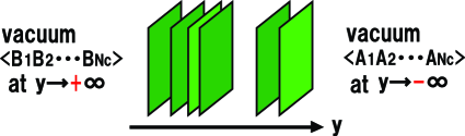
Therefore vacua are characterized by choosing labels out of flavors, corresponding to the nonvanishing color components . We shall denote this vacuum as . This vacuum is called color-flavor locked vacua. These discrete vacua allow domain walls which interpolate discretely different vacua at left and at right infinity . Therefore topological sectors for multi-walls are labeled by boundary conditions at and at .
Let us consider co-dimension one soliton such as walls. We assume that all fields depend only on the coordinate of one extra dimension , and assume the Poincaré invariance on the four-dimensional world volume of the soliton. The well-known Bogomol’nyi completion of the energy density gives
| (5) | |||||
where we have omitted total divergence terms which give only vanishing contributions for topological charges. Thus we obtain the Bogomol’nyi bound as the lower bound for the energy of the soliton. By saturating the complete squares, we obtain the BPS equation
| (6) | |||||
| (7) | |||||
| (8) | |||||
| (9) |
These conditions are precisely the condition for half of SUSY to be preserved by the soliton configuration. The energy (per unit world-volume of the wall) of the BPS saturated soliton for the topological sector labeled by is given by
| (10) |
2 BPS Wall Solutions
2.1 Solving BPS Equations
Let us first introduce an invertible complex matrix function defined by INOS1 , INOS2
| (11) |
By using this matrix function we obtain the solution of the hypermultiplet BPS equations (6) and (7) as
| (12) |
with the constant complex matrices as integration constants, which we call moduli matrices. We have used already the boundary condition for at .
Using the solution (12) of the hypermultiplet BPS equation, the remaining BPS equations (8) for the vector multiplets can be rewritten in terms of the matrix and the moduli matrix . The gauge transformations act on the matrix function as
| (13) |
Thus we define a gauge invariant quantity from as
| (14) |
The moduli matrix is also gauge invariant. The BPS equations (8) for vector multiplets can be rewritten in the following gauge invariant form
| (15) |
where the source term is given in terms of the moduli matrix as
| (16) |
We call Eq.(15) as the master equation for domain walls.
We should solve the master equation for a given moduli matrix . It has been conjectured that the solution of the master equation always exists and is unique, for any given moduli matrix INOS1 , INOS2 . If this is true, the moduli matrix is the necessary and sufficient data for the moduli of the solution. This conjecture has been proved for gauge thoeries recently SakaiYang . For non-Abelian gauge theories such as , the best evidence for the moduli matrix to be the necessary and sufficient data for the moduli, is given by the index theorem Sakai:2005sp : the number of independent parameters contained in the moduli matrix agrees precisely with that required by the index theorem. Additional evidence is provided by the exact solutions at strong gauge coupling limit and at discrete finite couplingIOS , where the solution of master equation indeed exists for a restricted class of moduli matrices INOS1 , INOS2 .
2.2 Total Moduli Space
The differential equation (11) defines the matrix function only up arbitrary complex integration constants. Therefore a set of the matrix function and the moduli matrix and another set give the same physical fields , provided they are related by
| (17) |
where . We call this symmetry as ‘world-volume symmetry’. This equivalence relation defines an equivalence class of moduli matrices, which is the genuinely independent moduli. Namely the moduli space for (multi-)wall solutions (including all possible boundary conditions) denoted by is topologically isomorphic to the complex Grassmann manifold:
| (18) |
whose complex dimension is given by . This is a compact (closed) set. On the other hand, one expects noncompact moduli parameters, such as positions of walls. The presence of noncompact moduli parameters and the compactness of the total moduli space can be consistently understood, if we note that the moduli space includes all topological sectors determined by different boundary conditions.
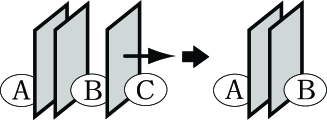
Suppose we have a three wall configuration connecting the vacuum A at left infinity to the vacuum C at right infinity through the next to right vacuum B. If we let the right-most wall to the right infinity, we eventually obtain a two wall configuration connecting the vacuum A to the vacuum B. In this way, we can obtain two wall toplogical sectors as boundaries of a three wall topological sector. From the above illusrative example, we can observe that the Grassmann manifold as the total moduli space can be decomposed into various topological sectors for BPS walls
| (19) |
One should note that the total moduli space also includes the vacuum states with no walls which correspond to points . These vacua are the only points where all SUSY are preserved . We can decompose in more detail according to topological sectors with specific boundary conditions
| (20) |
where denotes the moduli subspace of BPS (multi-)wall solutions for the topological sector of , and the sum is taken over the BPS sectors. Although each sector (except for vacuum states) is in general an open set containing noncompact moduli, the total space is compact.
2.3 Effective Lagrangian on BPS Walls
In order to obtain the low-energy effective field theory, we need to promote the moduli parameters to fields on the world-volume of walls Ma . It is again useful to use the solution (12) of the hypermultiplet BPS equation (6) in terms of the matrix function . By using the solution of the hypermultiplet BPS equation, we can rewrite the Lagrangian in terms of the gauge invariant matrix . By systematically expanding the Lagrangian in powers of the slow-movement parameter , we can retain up to two powers of . We find the resulting effective Lagrangian as
| (21) |
where is the tension of the BPS (multi-)wall in Eq.(10), and is the Kähler potential of moduli fields and
| (22) | |||||
We should replace the in (22) by the solution of the master equation (15).
It is interesting to observe that this Kähler potential serves as an action from which one can derive the master equation (15) by the usual minimal action principle. This fact can be explained if we use the superfield formulation for preserved four SUSY. By expanding the fundamental Lagrangian in powers of the slow-movement parameter , we find that the second hypermultiplet superfield and vector superfield become Lagrange multipliers. One can use the constraint equation resulting from integrating to obtain a Lagrangian in five dimensions amounting the Lagrangian for the remaining degree of freedom expressed in terms of the superfield . This is precisely the density of the Kähler potential in Eq.(22) before integrating over .
2.4 Exact Solution at Strong Coupling
In the strong gauge coupling limit , the master equation can be algebraically solved
| (23) |
With this solution, we can obtain by fixing a gauge. Then all the other fields such as and can also be obtained. There are two dimensionful parameters in the system: mass difference of hypermultiplets, and the gauge coupling times the square root of the Fayet-Iliopoulos parameter . The strong coupling limit actually implies the limit . This exact solution of master equation at corresponds to the gauge theory becoming a nonlinear sigma model (NLSM) whose target space is the cotangent bundle over the Grassmann manifold ANS . Since the Grassmann manifold is symmetric under the exchange of and with fixed , all the result are also symmetric under the exchange (actually the sign of the Fayet-Iliopoulos parameter should be changed). We call this as a duality.
Domain walls in this model can be realized as kinky D-brane connecting separated D()-branes in the type IIA/IIB string theory EINOOS . Dynamics of domain walls can be understood very easily by this brane configuration.
3 Global Structure of Wall Moduli Space
We have also studied slightly different model where several new features of walls are realized. This is a gauge theory with 4 hypermultiplets with unequal charges Eto:2005wf . The charges for these 4 hypermultiplets are given by
| (26) |
In the strong coupling limit , two vector multiplets produces two constraints, and gives a NLSM.
In order to study the constraints and the BPS flows for the multi-wall configurations, we define the following quantity as bilinears of scalar fields of the -th hypermultiplet
| (27) |
The conditions for SUSY vacua are given by
| (28) |
| (29) |
By studying the second constraint (29), we find that it is not allowed to have nonvanishing values of both (the first hypermultiplet) and (the second hypermultiplet) for each flavor. This implies that the BPS flows occur only in a submanifold with half of the total dimensions. We find that this moduli space of the BPS flows is precisely a special Lagrangian submanifold of the target space of the NLSM. We find that there are several special Lagrangian submanifolds for this target space of the NLSM. The total moduli space is obtained as the union of all these special Lagrangian submanifolds.
Because of two constraints from two gauge groups, we only need to use two out of four to describe the BPS flows. Since the BPS flows stop only at vacua, the first vacuum conditions (28) constitute boundaries of the BPS flows. Then the BPS flows for multi-wall configurations are restricted to closed polygons in the plane. We have shown three representative BPS flows depending on the mass assignments in Fig.3.
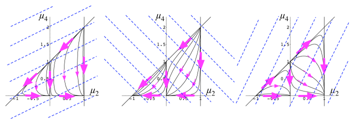
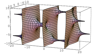
The case I) in Fig.3 shows that the three wall configuration has only two position moduli. This implies that there are repulsion and attraction between BPS walls, resulting in the phenomenon that the middle wall position of three walls is fixed. The case III) in Fig.3 shows that there is a transmutation of walls when two walls collide through moving in the moduli space. We have explicitly illustrated this movement in Fig.4 and 5.
We have also observed that the moduli space dimension can be larger than naively suggested by index theorem for walls connecting a particular set of vacua, for instance two vacua on in the case I.
4 Composite Solitons of Wall, Vortex and Monopole
4.1 Vortex Can Stretch between Walls
So far we have been considering walls which can appear in the Higgs phase of SUSY gauge theories. We can have solitons with more codimensions, such as vortices, monopoles, and instantons. If gauge group is unbroken, magnetic flux from a monopole can spread radially. However, if it is placed in the Higgs phase where there is no unbroken subgroups, magnetic flux has to be squeezed into a flux tube because of the Meissner effect, as illustrated in Fig.6. This composite soliton of monopoles and vortices has been found recently Tong:2003pz , Hanany:2004ea .
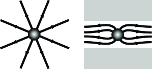
Therefore a monopole in the Higgs phase has to accompany vortices. Although both monopoles and vortices are BPS solitons, they preserve different halves of SUSY. We find that they preserve only a quarter of SUSY, and that walls are also allowed at the same time as composite soliton preserving of SUSY Isozumi:2004vg .
We assume that the configuration depends on (co-dimension three), and the Poincaré invariance in . By requring a SUSY to be conserved, we obtain the BPS equations for the composite solitons
| (30) | |||||
| (31) | |||||
| (32) |
where a contribution of vortex magnetic field is added to the wall BPS Eqs.(6), (8) together with the BPS equations for vortices. We obtain the BPS bound of the energy density as
| (33) | |||
where and are energy densities for walls, vortices and monopoles.
4.2 Solutions of BPS Equations
Eq.(32) guarantees the integrability condition of Eq.(31)
| (34) |
which allows us to define an invertible complex matrix function
| (35) | |||||
where , and . We can solve the hypermultiplet BPS Eq.(31) by
| (36) |
with the moduli matrix as an matrix as a holomorphic functionof . The remaining BPS equation for the vector multiplet scalar can be recast into the master equation for a -gauge invariant matrix function
| (37) |
with as a source term. This is an evolution equation along , with the initial data , giving all possible solutions of the BPS equation in the -dimensional configuration space. From the solution of the master equation for a given moduli matrix , we can obtain by fixing gauge, and then we also obtain and .
Assuming existence of unique solution of this equation for , the moduli matrix should contain the complete moduli of BPS soliton. Similarly to the wall case, we have also the world-volume symmetry
| (38) |
with an element of whose components are holomorphic in . Then the total moduli space including all topological sectors with different boundary conditions can be identified as a quotient of the holomorphic maps defined by
| (39) | |||
where is an complex matrix. In the strong coupling limit, the moduli space reduces to the space of all the holomorphic maps from the complex plane to the complex Grassmann manifold
| (40) |
4.3 Exact Solutions at Strong Coupling
If we take the strong coupling limit , the master equation (37) reduces to an algebraic equation
| (41) |
In this case, we can construct all solutions of the 1/4 BPS equations (30)-(32) exactly and explicitly.
Our construction produces rich contents, even for the gauge theories (). A general parametrization of the moduli matrix in this case is given by
| (42) |
In the strong coupling limit, the model reduces to a massive NLSM, where massive implies the presence of potential terms coming from the mass differences of hypermultipelts. The gauge invariant quantity is given in this case by
| (43) |
Since each term in the sum of corresponds to the weight of the vacuum, this can be regarded as a dependent multi-wall configuration. For each fixed , we have maximally walls at various points in . The position of the -th wall is given by . We now see that walls are bent for nonconstant . In particular, if has zeroes, they should correspond to walls extending to infinity: namely vortices are formed. More precisely we find that produces a configuration with vorticity at on the -th wall.
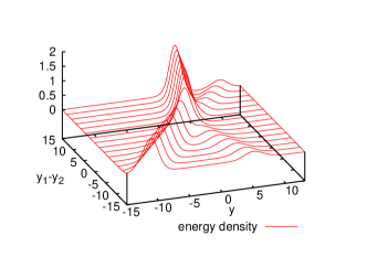
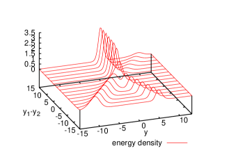
A typical composite soliton solution is depicted in Fig.7. We note that the monopole in Higgs phase is realized as a kink on vortex world volume. Let us emphasize that our method allows complete solutions of vortex stretching between two or more walls. Thus generalizing the D-brane soliton as a BIon on a single wall (D-brane).
More recently we have also constructed a similar composite soliton with codimension four. The instantons in the Higgs phase should also accompany voritces in the Higgs phase. Following the suggestion in Ref.Hanany:2004ea , we have obtained another BPS equation for the instantons in the Higgs phase, and have constructed a BPS solution EINOS . Moreover, we also observed that the monopole in the Higgs phase can be obtained by a Scherk-Schwarz dimensional reduction from the instantons in the Higgs phase. To illustrate the mechanism more explicitly, it is useful to consider the calorons in the Higgs phase, which are the periodic array of instantons in the Higgs phase. Although the solution can be understood physically as a semi-local vortex (lump) on a vortex, our solution is a genuine solution of the BPS equation, and not just a BPS solution of the effective theory on the vortex world volume.
References
- (1) P. Horava and E. Witten, Nucl. Phys. B460, 506 (1996) [arXiv:hep-th/9510209]; N. Arkani-Hamed, S. Dimopoulos and G. Dvali, Phys. Lett. B429, 263 (1998) [arXiv:hep-ph/9803315]; I. Antoniadis, N. Arkani-Hamed, S. Dimopoulos and G. Dvali, Phys. Lett. B436, 257 (1998) [arXiv:hep-ph/9804398]; L. Randall and R. Sundrum, Phys. Rev. Lett. 83, 3370 (1999) [arXiv:hep-ph/9905221]; Phys. Rev. Lett. 83, 4690 (1999) [arXiv:hep-th/9906064].
- (2) S. Dimopoulos and H. Georgi, Nucl. Phys. B193, 150 (1981); N. Sakai, Z. f. Phys. C11, 153 (1981); E. Witten, Nucl. Phys. B188, 513 (1981); S. Dimopoulos, S. Raby and F. Wilczek, Phys. Rev. D24, 1681 (1981).
- (3) E. Witten and D. Olive, Phys. Lett. B78, 97 (1978).
- (4) N. S. Manton, Phys. Lett. B110, 54 (1982).
- (5) M. Arai, M. Nitta and N. Sakai, Prog. Theor. Phys. 113, 657 (2005) [arXiv:hep-th/0307274].
- (6) Y. Isozumi, M. Nitta, K. Ohashi and N. Sakai, Phys. Rev. Lett. 93 161601 (2004) [arXiv:hep-th/0404198].
- (7) Y. Isozumi, M. Nitta, K. Ohashi and N. Sakai, Phys. Rev. D70 (2004) 125014 [arXiv:hep-th/0405194].
- (8) N. Sakai and Y. Yang, arXiv:hep-th/0505136.
- (9) N. Sakai and D. Tong, JHEP 0503, 019 (2005) [arXiv:hep-th/0501207].
- (10) Y. Isozumi, K. Ohashi, and N. Sakai, JHEP 11, 060 (2003) [arXiv:hep-th/0310189].
- (11) M. Eto, Y. Isozumi, M. Nitta, K. Ohashi, K. Ohta and N. Sakai, Phys. Rev. D71, 125006 (2005) [arXiv:hep-th/0412024].
- (12) M. Eto, Y. Isozumi, M. Nitta, K. Ohashi, K. Ohta, N. Sakai and Y. Tachikawa, Phys. Rev. D71, 105009 (2005) [arXiv:hep-th/0503033].
- (13) D. Tong, Phys. Rev. D69, 065003 (2004) [arXiv:hep-th/0307302]; R. Auzzi, S. Bolognesi, J. Evslin and K. Konishi, Nucl. Phys. B686, 119 (2004) [arXiv:hep-th/0312233]; M. Shifman and A. Yung, Phys. Rev. D70, 045004 (2004) [arXiv:hep-th/0403149]; R. Auzzi, S. Bolognesi and J. Evslin, JHEP 0502, 046 (2005) [arXiv:hep-th/0411074]; M. A. C. Kneipp and P. Brockill, Phys. Rev. D64, 125012 (2001) [arXiv:hep-th/0104171].
- (14) A. Hanany and D. Tong, JHEP 0404, 066 (2004) [arXiv:hep-th/0403158].
- (15) Y. Isozumi, M. Nitta, K. Ohashi and N. Sakai, Phys. Rev. D71, 065018 (2005) [arXiv:hep-th/0405129].
- (16) M. Eto, Y. Isozumi, M. Nitta, K. Ohashi and N. Sakai, Phys. Rev. D72, 025011 (2005) [arXiv:hep-th/0412048].