Recursive method to obtain the parametric representation of a generic Feynman diagram

Abstract

A recursive algebraic method which allows to obtain the Feynman or Schwinger parametric representation of a generic $L$-loops and $(E+1)$ external lines diagram, in a scalar $\phi^{3}\oplus\phi^{4}$ theory, is presented. The  representation is obtained starting from an Initial Parameters Matrix (IPM), which relates the scalar products between internal and external momenta, and which appears explicitly when this parametrization is applied to the momentum space representation of the graph. The final product is an algorithm that can be easily programmed, either in a computer programming language (C/C++, Fortran,…) or in a symbolic calculation package (Maple, Mathematica,…).

PACS: 11.25 Db; 12.38 Bx

Keywords: Perturbation theory; Feynman diagrams; Feynman parameters, Schwinger parameters; Quadratic forms.

1 Introduction

An important mathematical problem in Elementary Particle Physics is the evaluation of Feynman integrals, which usually appear in the perturbative treatment of quantum field theory amplitudes. Besides the intrinsic difficulty in solving the integrals associated to a specific graph, in general the number of diagrams grows rapidly when the number of loops is increased, which makes necessary to develop methods that allow for the automatization both in the generation and the evaluation of such integrals. The first problem that we face in dealing with a Feynman diagram is to decide which integral representation is the most convenient in order to start the process for finding a solution. Among the different alternatives we have the parametric representations, in particular the Feynman parametrization (FP) ([1],[2],[3]) and the Schwinger parametrization ($\alpha$-parameters) ([1],[3], [4]) , which allow for the transformation of the loop integrals into scalar multidimensional integrals. These representations also permit, using dimensional regularization, for a clear and direct analysis of the convergence problem, and furthermore the property of Lorentz invariance is also explicit in these representations. Recently very efficient analytical and numerical methods for evaluating loop integrals have been proposed, which use as a starting point a scalar representation. In particular the Mellin-Barnes [5] representation allows for analytical solutions of complicated diagrams, starting from a Feynman parameters integral. In numerical calculations an excellent technique is the so called Sector Decomposition ([5],[6],[7]), which allows to find the Laurent series of the diagram in terms of the dimensional regulator $(\epsilon)$, systematically separating by integration sectors the divergences in the Feynman parameters integral. From this point of view it would be convenient to find an accessible way for obtaining the above mentioned parametric representations. Although at present there are in the literature algorithms of topological nature [8], its implementation is quite complicated from the point of view of the automatization.

For simplicity we will consider here a scalar theory, although the generalization to fermionic theories is straightforward. The final result is a simple algorithm which allows to find the parametric representation of any loop integral, and which can be easily programmed computationally. The basis of this formalism is a generalization of the completion of squares procedure used in mathematics structures denominated Quadratic Forms ([9],[10],[11]) , which are precisely those that appear when applying a scalar parametrization to the momentum space integral representations. In essence the expression of the form $\mathbf{Q}^{t}\mathbf{MQ}$ is a quadratic form, where $\mathbf{Q}$ is an $(L+E)-vector$ that contains all the independent internal and external momenta of the graph and $\mathbf{M}$ is a matrix denominated Initial Parameters Matrix (IPM). The end result of the process is a recurrence equation that is the support of the algorithm.

This study is developed making emphasis on the differences that exist in the way of finding the parametric representation and the resultant mathematical structure, between the usual method and the one proposed here. We also find that the parametric representation can be expressed in two equivalent and directly related ways, the first one in terms of matrix elements generated by recursion starting from the IPM and the second in terms of determinants of submatrices of the IPM. The relationship between both representations is demonstrated in appendices A and  B. Finally, two detailed examples are presented, illustrating the procedure for obtaining the parametric representation of a Feynman diagram, and which allow to compare in practical terms the usual method and the one proposed here. We also add the explicit code to generate the recursive elements of the scalar representation, in the symbolic calculation package Maple.

2 The formalism

Let us consider a generic topology $G$ that represents a Feynman diagram in a scalar theory, and suppose that this graph is composed of $N$ propagators or internal lines, $L$ loops (associated to independent internal momenta $\underline{q}=\left\{q_{1},...,q_{L}\right\}$, and $E$ independent external momenta $\underline{p}=\left\{p_{1},...,p_{E}\right\}$. Each propagator or internal line is characterized by an arbitrary and in general different mass, $\underline{m}=\left\{m_{1},...,m_{N}\right\}$.

Using the prescription of dimensional regularization we can write the momentum space integral expression that represents the diagram in $D=4-2\epsilon$ dimensions as:

$$G=G(\underline{p},\underline{m})=\mathop{\displaystyle\int}\frac{d^{D}q_{1}}{i\pi^{D/2}}...\frac{d^{D}q_{L}}{i\pi^{D/2}}\frac{1}{(B_{1}^{2}-m_{1}^{2}+i\delta)^{\nu_{1}}}...\frac{1}{(B_{N}^{2}-m_{N}^{2}+i\delta)^{\nu_{N}}}.$$ (1)

In this expression the symbol $B_{j}$ represents the momentum of the $j$ propagator or internal line, which in general depends on a linear combination of external $\left\{\underline{p}\right\}$ and internal $\left\{\underline{q}\right\}$ momenta: $B_{j}=B_{j}(\underline{q},\underline{p})$.

We also define the set $\underline{\nu}=\left\{\nu_{1},...,\nu_{N}\right\}$ as the set of powers of the propagators, which in general can take arbitrary values.

Here we will study two well-known parametric representations: the Feynman parametrization and the Schwinger parametrization. In the next sections we will show how to express equation $\left(\ref{a}\right)$ in terms of these two scalar representations. The technique consists in transforming the product of denominators in $\left(\ref{a}\right)$ into a sum through the use of an integral identity.

2.1 Momentum representation and his scalar parametrization

2.1.1 Feynman Parametrization

Using the identity:

$$\dfrac{1}{\mathop{\textstyle\prod}\limits_{j=1}^{N}A_{j}^{\nu_{j}}}=\dfrac{\Gamma(\nu_{1}+...+\nu_{N})}{\Gamma(\nu_{1})...\Gamma(\nu_{N})}\mathop{\displaystyle\int}\limits_{0}^{1}dx_{1}...dx_{N}\;\delta(1-\mathop{\textstyle\sum}\limits_{j=1}^{N}x_{j})\dfrac{\mathop{\textstyle\prod}\limits_{j=1}^{N}x_{j}^{\nu_{j}-1}}{\left[\mathop{\textstyle\sum}\limits_{j=1}^{N}x_{j}A_{j}\right]^{\nu_{1}+...+\nu_{N}}}$$ (2)

and after defining $A_{j}=\left(B_{j}^{2}-m_{j}^{2}\right)$, we can replace $\left(\ref{n}\right)$ into equation $\left(\ref{a}\right)$ and thus obtain the following generic result:

$$G=\dfrac{\Gamma(N_{\nu})}{\Gamma(\nu_{1})...\Gamma(\nu_{N})}\mathop{\displaystyle\int}\limits_{0}^{1}d\overrightarrow{x}\,\delta(1-\mathop{\textstyle\sum}\limits_{j=1}^{N}x_{j})\int\frac{\mathop{\textstyle\prod}\limits_{j=1}^{L}d^{D}q_{j}}{\left(i\pi^{D/2}\right)^{L}}\dfrac{1}{\left[\mathop{\textstyle\sum}\limits_{j=1}^{N}x_{j}B_{j}^{2}-\mathop{\textstyle\sum}\limits_{j=1}^{N}x_{j}m_{j}^{2}\right]^{N_{\nu}}}.$$ (3)

For simplicity, from now on we use the following notation: $d\overrightarrow{x}=dx_{1}...dx_{N}\mathop{\textstyle\prod}\limits_{j=1}^{N}x_{j}^{\nu_{j}-1}$ y $N_{\nu}=\left(\nu_{1}+...+\nu_{N}\right)$.

2.1.2 Schwinger Parametrization

The fundamental identity for this specific parametrization is given by the equation:

$$\dfrac{1}{A_{j}^{\nu_{j}}}=\int\limits_{0}^{\infty}dx_{j}\,x_{j}^{\nu_{j}-1}\exp(-x_{j}A_{j}),$$ (4)

which allows, after replacing $A_{j}=\left(B_{j}^{2}-m_{j}^{2}\right)$, to express equation $\left(\ref{a}\right)$ in the following general form:

$$G=\dfrac{1}{\Gamma(\nu_{1})...\Gamma(\nu_{N})}\mathop{\displaystyle\int}\limits_{0}^{\infty}d\overrightarrow{x}\exp\left(\mathop{\textstyle\sum}\limits_{j=1}^{N}x_{j}m_{j}^{2}\right)\mathop{\displaystyle\int}\frac{\mathop{\textstyle\prod}\limits_{j=1}^{L}d^{D}q_{j}}{\left(i\pi^{D/2}\right)^{L}}\exp\left(-\mathop{\textstyle\sum}\limits_{j=1}^{N}x_{j}B_{j}^{2}\right).$$ (5)

The next step is integrating $\left(\ref{b}\right)$ and $\left(\ref{c}\right)$ with respect to the internal momenta, obtaining in this way the corresponding scalar parametrization.

2.2 Loop momenta integration and parametric representation (Usual method)

The usual way to integrate over internal momenta consists in expanding the sum $\mathop{\textstyle\sum}\nolimits_{j=1}^{N}x_{j}B_{j}^{2}$ and reorder it in the following manner:

$$\mathop{\textstyle\sum}\limits_{j=1}^{N}x_{j}B_{j}^{2}=\mathop{\textstyle\sum}\limits_{i=1}^{L}\mathop{\textstyle\sum}\limits_{j=1}^{L}q_{i}A_{ij}q_{j}-2\mathop{\textstyle\sum}\limits_{i=1}^{L}k_{i}q_{i}+J,$$ (6)

or expressed more compactly in matrix form:

$$\mathop{\textstyle\sum}\limits_{j=1}^{N}x_{j}B_{j}^{2}=\mathbf{q}^{t}\mathbf{Aq}-2\mathbf{k}^{t}\mathbf{q}+J$$ (7)

where the following quantities have been defined:

$\mathbf{A}\implies$ Symmetric matrix of dimension $L\times L$, whose elements are functions of the parameters $\underline{x}$ only: $\mathbf{A=A}\left(\underline{x}\right)$.

$\mathbf{q}\implies$ $L-vector$, whose components are the loop or internal 4-vector momenta: $\mathbf{q}\ =\ \left[q_{1}\;...q_{L}\right]^{t}$.

$\mathbf{k}$ $\implies$ $L-vector$, whose components are linear combinations of external momenta, with coefficients that are functions of the parameters $\underline{x}$ only, so $\mathbf{k}=\mathbf{k}\left(\underline{x},\underline{p}\right)$.

$J\implies$ Scalar term, which is a linear combination of scalar products of external momenta, with coefficients that depend on the parameters $\underline{x}$ only, $J=J\left(\underline{x},\underline{p}\right)$.

Evidently the specific form of each of these quantities depends on the topology of the corresponding diagram, and is made explicit once the parametrization formula is applied to equation $\left(\ref{a}\right)$. With the reordering presented in $\left(\ref{h}\right)$, we can write both parametrizations and their respective solutions after performing the momenta integrations.

2.2.1 Feynman parametrization

$$G=\dfrac{\Gamma(N_{\nu})}{\Gamma(\nu_{1})...\Gamma(\nu_{N})}\mathop{\displaystyle\int}\limits_{0}^{1}d\overrightarrow{x}\,\delta(1-\mathop{\textstyle\sum}\limits_{j=1}^{N}x_{j})\mathop{\displaystyle\int}\frac{\mathop{\textstyle\prod}\limits_{j=1}^{L}d^{D}q_{j}}{\left(i\pi^{D/2}\right)^{L}}\frac{1}{\left[\mathbf{q}^{t}\mathbf{Aq}-2\mathbf{k}^{t}\mathbf{q}+J-\mathop{\textstyle\sum}\limits_{j=1}^{N}x_{j}m_{j}^{2}\right]^{N_{\nu}}},$$ (8)

which once the loop momenta integral are performed, gives finally the Feynman parametric representation:

$$G=\dfrac{(-1)^{N_{\nu}}\Gamma(N_{\nu}-\frac{LD}{2})}{\Gamma(\nu_{1})...\Gamma(\nu_{N})}\mathop{\displaystyle\int}\limits_{0}^{1}d\overrightarrow{x}\;\delta(1-\mathop{\textstyle\sum}\limits_{j=1}^{N}x_{j})\dfrac{\left[\det\mathbf{A}\right]^{N_{\nu}-(L+1)\frac{D}{2}}}{\left[\det\mathbf{A}\left(\mathop{\textstyle\sum}\limits_{j=1}^{N}x_{j}m_{j}^{2}-J+\mathbf{k}^{t}\mathbf{A}^{-1}\mathbf{k}\right)\right]^{N_{\nu}-\frac{LD}{2}}}.$$ (9)

2.2.2 Schwinger parametrization

$$G=\dfrac{1}{\Gamma(\nu_{1})...\Gamma(\nu_{N})}\mathop{\displaystyle\int}\limits_{0}^{\infty}d\overrightarrow{x}\,\exp\left(\mathop{\textstyle\sum}\limits_{j=1}^{N}x_{j}m_{j}^{2}-J\right)\mathop{\displaystyle\int}\frac{\mathop{\textstyle\prod}\limits_{j=1}^{L}d^{D}q_{j}}{\left(i\pi^{D/2}\right)^{L}}\exp\left(-\mathbf{q}^{t}\mathbf{Aq+}2\mathbf{k}^{t}\mathbf{q}\right).$$ (10)

In an analogous way, after integration over internal momenta we obtain Schwinger’s parametrization of $G$:

$$G=\dfrac{(-1)^{\frac{LD}{2}}}{\Gamma(\nu_{1})...\Gamma(\nu_{N})}\mathop{\displaystyle\int}\limits_{0}^{\infty}d\overrightarrow{x}\,\,\left[\det\mathbf{A}\right]^{-\frac{D}{2}}\exp\left(\mathop{\textstyle\sum}\limits_{j=1}^{N}x_{j}m_{j}^{2}-J+\mathbf{k}^{t}\mathbf{A}^{-1}\mathbf{k}\right).$$ (11)

The techniques for solving the momenta integrals in $\left(\ref{d}\right)$ and $\left(\ref{e}\right)$ can be found in detail in the literature, both for the Feynman parametrization case([1],[2]), as well as for the Schwinger[1] case. This last one is usually solved using products of $D$-dimensional gaussian integrals, in Minskowski or Euclidian spaces.

Notice that in both parametrizations (equations $\left(\ref{t}\right)$ and $\left(\ref{ee}\right)$) it is necessary to evaluate a matrix product that involves an inverse matrix calculation, which makes the procedure not so straightforward to implement.

2.3 Alternative procedure for obtaining the Parametric Representation ( I )

Starting from equations $\left(\ref{b}\right)$ and $\left(\ref{c}\right)$, we can choose to represent the term $\mathop{\textstyle\sum}\nolimits_{j=1}^{N}x_{j}B_{j}^{2}$ as a function of both internal and external scalar products, related through the symmetric matrix $\mathbf{M}^{\left(1\right)}$, which we will call Initial Parameters Matrix (MPI). The dimension of this matrix is therefore $\left(L+E\right)\times\left(L+E\right)$.

For convenience, let us define the momentum:

$$Q_{j}=\left\{\begin{array}[]{ccc}q_{j}&if&L\geq j\geq 1\\ p_{j-L}&if&E\geq j>L\end{array}\right.$$ (12)

and the $\left(L+E\right)-vector$ $\mathbf{Q=[}Q_{1}\quad Q_{2}\quad...Q_{(L+E)}]^{t}$.

Using this definition we can reorder the sum $\mathop{\textstyle\sum}\nolimits_{j=1}^{N}x_{j}B_{j}^{2}$, and rewrite it as:

$$\mathop{\textstyle\sum}\limits_{j=1}^{N}x_{j}B_{j}^{2}=\mathop{\textstyle\sum}\limits_{i=1}^{L+E}\mathop{\textstyle\sum}\limits_{j=1}^{L+E}Q_{i}M_{ij}^{\left(1\right)}Q_{j}=\mathbf{Q}^{t}\mathbf{M}^{\left(1\right)}\mathbf{Q},$$ (13)

where $\mathbf{M}^{\left(1\right)}$ is clearly a matrix that only depends on parameters.

The difference in the matrix structure, with respect to the usual method of finding the parametric representation, is that here we include both external and internal momenta in the same quadratic representation, and not only the internal ones as in the usual case we presented above(see equation$\left(\ref{h}\right)$), which produces matrix $\mathbf{\ A}$. In fact, matrix $\mathbf{A}$ is a submatrix of $\mathbf{M}^{\left(1\right)}$, which already shows an important difference in the parametrization starting point, with respect to the usual method. More explicitly we have that:

$$A=\left(\begin{array}[]{ccc}a_{11}&\ldots&a_{1L}\\ \vdots&&\vdots\\ a_{L1}&\ldots&a_{LL}\end{array}\right)$$ (14)

whereas the Initial Parameters Matrix is given by:

$$M^{\left(1\right)}=\left(\begin{array}[]{ll}\begin{array}[]{lll}a_{11}&\ldots&a_{1L}\\ \vdots&&\quad\vdots\\ a_{L1}&\ldots&a_{LL}\end{array}&\begin{array}[]{lll}&\ldots&M_{{}_{1\left(L+E\right)}}^{(1)}\\ &&\\ &&\qquad\vdots\end{array}\\ \begin{array}[]{lll}&&\\ \vdots&&\\ M_{\left({}_{L+E}\right)1}^{(1)}&&\ldots\end{array}&\begin{array}[]{lll}\ddots&&\\ &&\\ &&M_{{}_{\left(L+E\right)\left(L+E\right)}}^{(1)}\end{array}\end{array}\right)$$ (15)

$$\text{con }M_{ij}^{(1)}=\left\{\begin{array}[]{ll}a_{ij}&\text{if }L\geq i\geq 1,L\geq j\geq 1\\ M_{ij}^{(1)}&\text{in other cases.}\end{array}\right.$$ (16)

In appendix A we show a generalization of the square completion method for diagonalizing  Quadratic Forms, which is what appears when we parametrize the loop integrals. Looking at the definition of $\mathbf{Q}$ in $\left(\ref{o}\right)$, and since we have to integrate only the first $L$ momenta, only the main $L\times L$ submatrix has to be diagonalized; that is, we need to perform a change of variables in the first $L$ momenta of the $(L+E)-vector$ $\mathbf{Q}$. This can be summarized in the following expression:

$$\mathbf{Q}^{t}\mathbf{M}^{\left(1\right)}\mathbf{Q=}\mathop{\textstyle\sum}\limits_{j=1}^{L}M_{jj}^{\left(j\right)}\widetilde{Q}_{j}^{2}+\mathop{\textstyle\sum}\limits_{i=L+1}^{L+E}\mathop{\textstyle\sum}\limits_{j=L+1}^{L+E}Q_{i}M_{ij}^{(L+1)}Q_{j}.$$ (17)

Using the definition $\left(\ref{o}\right)$, the double sum can be expressed in terms of the external momenta:

$$\mathop{\textstyle\sum}\limits_{i=L+1}^{L+E}\mathop{\textstyle\sum}\limits_{j=L+1}^{L+E}Q_{i}M_{ij}^{\left(L+1\right)}Q_{j}=\mathop{\textstyle\sum}\limits_{i=1}^{E}\mathop{\textstyle\sum}\limits_{j=1}^{E}M_{\left(L+i\right)\left(L+j\right)}^{\left(L+1\right)}\,p_{i}.p_{j}\;.$$ (18)

Thus the quadratic form of the momenta $\mathbf{Q}$ can be written as:

$$\mathbf{Q}^{t}\mathbf{M}^{\left(1\right)}\mathbf{Q=}\mathop{\textstyle\sum}\limits_{j=1}^{L}M_{jj}^{\left(j\right)}\widetilde{Q}_{j}^{2}+\mathop{\textstyle\sum}\limits_{i=1}^{E}\mathop{\textstyle\sum}\limits_{j=1}^{E}M_{\left(L+i\right)\left(L+j\right)}^{\left(L+1\right)}\,p_{i}.p_{j}\;.$$ (19)

When the square completion procedure is performed to the quadratic form $\left(\ref{p}\right)$, the linear transformation for each internal momentum is given in general by an expression of the form:

$$\widetilde{Q}_{j}=Q_{j}+f\left(\underline{x},Q_{j+1},...,Q_{L+E}\right)\text{ \ \ with }j=1,...,L$$ (20)

whose Jacobian is equal to unity. The matrix elements of the type $M_{ij}^{\left(k\right)}$ are defined through the following recursion relation (see appendix A):

$$\begin{array}[]{cc}M_{ij}^{\left(k+1\right)}=&\left\{\begin{array}[]{ll}0&\text{, if }\ i<(k+1)\ \vee\ j<(k+1)\\ M_{ij}^{\left(k\right)}-\dfrac{M_{ik}^{\left(k\right)}M_{kj}^{\left(k\right)}}{M_{kk}^{\left(k\right)}}&\text{, in other cases.}\end{array}\right.\end{array}$$ (21)

Therefore in a generic way the first $L$ momenta of the vector $\mathbf{Q}$ have been diagonalized, using the square completion method. Once this has been done, we are in a position to obtain the desired parametric representation.

2.3.1 Feynman Parametrization in terms of the matrix elements $M_{ij}^{(k)}$

Using equation $\left(\ref{p}\right)$, the identity $\left(\ref{b}\right)$ can be written in terms of the vector $\mathbf{Q}$, and thus we get the following equality:

$$G=\dfrac{\Gamma(N_{\nu})}{\Gamma(\nu_{1})...\Gamma(\nu_{N})}\mathop{\displaystyle\int}\limits_{0}^{1}d\overrightarrow{x}\,\delta(1-\mathop{\textstyle\sum}\limits_{j=1}^{N}x_{j})\mathop{\displaystyle\int}\frac{\mathop{\textstyle\prod}\limits_{j=1}^{L}d^{D}Q_{j}}{\left(i\pi^{D/2}\right)^{L}}\dfrac{1}{\left[\mathbf{Q}^{t}\mathbf{M}^{\left(1\right)}\mathbf{Q}-\mathop{\textstyle\sum}\limits_{j=1}^{N}x_{j}m_{j}^{2}\right]^{N_{\nu}}}.$$ (22)

Then we expand the denominator of the previous equation, using equality $\left(\ref{i}\right)$, and therefore we obtain a more explicit expression with respect to the integration variables $\widetilde{Q}_{j}$:

$$G=\dfrac{\Gamma(N_{\nu})}{\Gamma(\nu_{1})...\Gamma(\nu_{N})}\mathop{\displaystyle\int}\limits_{0}^{1}d\overrightarrow{x}\,\delta(1-\mathop{\textstyle\sum}\limits_{j=1}^{N}x_{j})\mathop{\displaystyle\int}\frac{\mathop{\textstyle\prod}\limits_{j=1}^{L}d^{D}\widetilde{Q}_{j}}{\left(i\pi^{D/2}\right)^{L}}\frac{1}{\left[\mathop{\textstyle\sum}\limits_{j=1}^{L}M_{jj}^{\left(j\right)}\widetilde{Q}_{j}^{2}-\Delta\right]^{N_{\nu}}},$$ (23)

where it has been defined

$$\Delta=\mathop{\textstyle\sum}\limits_{j=1}^{N}x_{j}m_{j}^{2}-\mathop{\textstyle\sum}\limits_{i,j=1}^{E}M_{\left(L+i\right)\left(L+j\right)}^{\left(L+1\right)}\,p_{i}.p_{j}\;.$$ (24)

If we now make a second change of variables, such that:

$$\widetilde{\widetilde{Q}}_{j}=\left[M_{jj}^{\left(j\right)}\right]^{1/2}\widetilde{Q}_{j}\Longrightarrow\widetilde{Q}_{j}=\left[M_{jj}^{\left(j\right)}\right]^{-1/2}\widetilde{\widetilde{Q}}_{j},$$ (25)

then:

$$d^{D}\widetilde{Q}_{j}=d^{D}\left(\left[M_{jj}^{\left(j\right)}\right]^{-1/2}\widetilde{\widetilde{Q}}_{j}\right)=\left[M_{jj}^{\left(j\right)}\right]^{-D/2}d^{D}\widetilde{\widetilde{Q}}_{j}\qquad\text{con }j=1,...,L$$ (26)

and replacing this in equation $\left(\ref{f}\right)$, we will have the following transformed loop momenta integral:

$$G=\frac{\Gamma(N_{\nu})}{\Gamma(\nu_{1})...\Gamma(\nu_{N})}\mathop{\displaystyle\int}\limits_{0}^{1}d\overrightarrow{x}\,\delta(1-\mathop{\textstyle\sum}\limits_{j=1}^{N}x_{j})\mathop{\displaystyle\int}\frac{\mathop{\textstyle\prod}\limits_{j=1}^{L}d^{D}\widetilde{\widetilde{Q}}_{j}}{\left(i\pi^{D/2}\right)^{L}}\frac{\left[M_{11}^{\left(1\right)}...M_{LL}^{\left(L\right)}\right]^{\frac{-D}{2}}}{\left[\mathop{\textstyle\sum}\nolimits_{j=1}^{L}\widetilde{\widetilde{Q_{j}^{2}}}-\Delta\right]^{N_{\nu}}}.$$ (27)

In order to perform the integral with respect to the variables $\widetilde{\widetilde{\mathbf{Q}}}_{j}$, let us define now the $Hipermomentum\quad\mathbf{R}$  of $\left(LD\right)$ components in Minkowski space, such that:

$$R^{2}=\mathop{\textstyle\sum}\nolimits_{j=1}^{L}\widetilde{\widetilde{Q_{j}^{2}}}$$ (28)

$$d^{D}\widetilde{\widetilde{Q}}_{1}...d^{D}\widetilde{\widetilde{Q}}_{L}=d^{LD}R.$$ (29)

Then the expression $\left(\ref{g}\right)$ is reduced to:

$$G=\frac{\Gamma(N_{\nu})}{\Gamma(\nu_{1})...\Gamma(\nu_{N})}\mathop{\displaystyle\int}\limits_{0}^{1}d\overrightarrow{x}\,\delta(1-\mathop{\textstyle\sum}\limits_{j=1}^{N}x_{j})\mathop{\displaystyle\int}\frac{d^{LD}R}{\left(i\pi^{\frac{D}{2}}\right)^{L}}\frac{\left[M_{11}^{\left(1\right)}...M_{LL}^{\left(L\right)}\right]^{\frac{-D}{2}}}{\left(R^{2}-\Delta\right)^{N_{\nu}}}.$$ (30)

The solution of this integral, with respect to the Hipermomentum $\mathbf{R}$, can be found using the following identity:

$$\mathop{\displaystyle\int}\dfrac{d^{LD}R}{\left(i\pi^{\frac{D}{2}}\right)^{L}}\frac{1}{\left[R^{2}-\bigtriangleup\right]^{N_{\nu}}}=\left(-1\right)^{N_{\nu}}\frac{\Gamma(N_{\nu}-\frac{LD}{2})}{\Gamma(N_{\nu})}\frac{1}{\bigtriangleup^{N_{\nu}-\frac{LD}{2}}},$$ (31)

and which finally applied to equation $\left(\ref{j}\right)$ gives us the scalar integral, that is the Feynman parametric representation of $G$:

$$G=\dfrac{\left(-1\right)^{N_{\nu}}\Gamma(N_{\nu}-\frac{LD}{2})}{\Gamma(\nu_{1})...\Gamma(\nu_{N})}\mathop{\displaystyle\int}\limits_{0}^{1}d\overrightarrow{x}\;\delta(1-\mathop{\textstyle\sum}\limits_{j=1}^{N}x_{j})\dfrac{\left[M_{11}^{\left(1\right)}...M_{LL}^{\left(L\right)}\right]^{\frac{-D}{2}}}{\left[\mathop{\textstyle\sum}\limits_{j=1}^{N}x_{j}m_{j}^{2}-\mathop{\textstyle\sum}\limits_{i,j=1}^{E}M_{\left(L+i\right)\left(L+j\right)}^{\left(L+1\right)}\,p_{i}.p_{j}\right]^{N_{\nu}-\frac{LD}{2}}},$$ (32)

where the matrix elements $M_{\left(L+i\right)\left(L+j\right)}^{\left(L+1\right)}$ can be easily obtained from the MPI using the recursion formula:

$$M_{\left(L+i\right)\left(L+j\right)}^{\left(L+1\right)}=M_{(L+i)(L+j)}^{\left(L\right)}-\dfrac{M_{(L+i)L}^{\left(L\right)}M_{L(L+j)}^{\left(L\right)}}{M_{LL}^{\left(L\right)}}.$$ (33)

2.3.2 Schwinger Parametrization in terms of the matrix elements $M_{ij}^{(k)}$

Analogously, using equation $\left(\ref{p}\right)$, the identity $\left(\ref{c}\right)$ can be written in terms of the vector $\mathbf{Q}$ as:

$$G=\dfrac{1}{\Gamma(\nu_{1})...\Gamma(\nu_{N})}\mathop{\displaystyle\int}\limits_{0}^{\infty}d\overrightarrow{x}\,\exp\left(\mathop{\textstyle\sum}\limits_{j=1}^{N}x_{j}m_{j}^{2}\right)\mathop{\displaystyle\int}\frac{\mathop{\textstyle\prod}\limits_{j=1}^{L}d^{D}Q_{j}}{\left(i\pi^{D/2}\right)^{L}}\exp\left(-\mathop{\textstyle\sum}\limits_{j=1}^{N}\mathbf{Q}^{t}\mathbf{M}^{\left(1\right)}\mathbf{Q}\right),$$ (34)

or equivalently, using the expansion given in equation $\left(\ref{i}\right)$, we get:

$$G=\dfrac{1}{\Gamma(\nu_{1})...\Gamma(\nu_{N})}\mathop{\displaystyle\int}\limits_{0}^{\infty}d\overrightarrow{x}\,\exp\left(\Delta\right)\mathop{\displaystyle\int}\frac{\mathop{\textstyle\prod}\limits_{j=1}^{L}d^{D}\widetilde{Q_{j}}}{\left(i\pi^{D/2}\right)^{L}}\exp\left(-\mathop{\textstyle\sum}\limits_{j=1}^{L}M_{jj}^{\left(j\right)}\widetilde{Q}_{j}^{2}\right),$$ (35)

where again we have defined:

$$\Delta=\mathop{\textstyle\sum}\limits_{j=1}^{N}x_{j}m_{j}^{2}-\mathop{\textstyle\sum}\limits_{i,j=1}^{E}M_{\left(L+i\right)\left(L+j\right)}^{\left(L+1\right)}\,p_{i}.p_{j}.$$ (36)

Now we can solve the momentum integral:

$$\mathop{\displaystyle\int}\frac{\mathop{\textstyle\prod}\limits_{j=1}^{L}d^{D}\widetilde{Q_{j}}}{\left(i\pi^{D/2}\right)^{L}}\exp\left(-\mathop{\textstyle\sum}\limits_{j=1}^{L}M_{jj}^{\left(j\right)}\widetilde{Q}_{j}^{2}\right)=\mathop{\displaystyle\int}\dfrac{d^{D}\widetilde{Q}_{1}}{i\pi^{D/2}}\exp\left(-M_{11}^{\left(1\right)}\widetilde{Q}_{1}^{2}\right)...\mathop{\displaystyle\int}\dfrac{d^{D}\widetilde{Q}_{L}}{i\pi^{D/2}}\exp\left(-M_{LL}^{\left(L\right)}\widetilde{Q}_{L}^{2}\right).$$ (37)

In order to find a solution of this integral we make use of the Minkowski space identity:

$$\mathop{\displaystyle\int}\dfrac{d^{D}\widetilde{Q}_{j}}{\left(i\pi^{\frac{D}{2}}\right)}\exp\left(-M_{jj}^{\left(j\right)}\widetilde{Q}_{j}^{2}\right)=\frac{\left(-1\right)^{\frac{D}{2}}}{\left[M_{jj}^{\left(j\right)}\right]^{\frac{D}{2}}},$$ (38)

which will allow to evaluate $\left(\ref{q}\right)$. Replacing afterwards this result in $\left(\ref{r}\right)$, we obtain finally the Schwinger parametric representation for the generic graph $G$:

$$G=\dfrac{(-1)^{\frac{LD}{2}}}{\Gamma(\nu_{1})...\Gamma(\nu_{N})}\mathop{\displaystyle\int}\limits_{0}^{\infty}d\overrightarrow{x}\,\,\left[M_{11}^{\left(1\right)}...M_{LL}^{\left(L\right)}\right]^{-\frac{D}{2}}\exp\left(\mathop{\textstyle\sum}\limits_{j=1}^{N}x_{j}m_{j}^{2}-\mathop{\textstyle\sum}\limits_{i,j=1}^{E}M_{\left(L+i\right)\left(L+j\right)}^{\left(L+1\right)}\,p_{i}.p_{j}\right)$$ (39)

in terms again of the matrix elements $M_{\left(L+i\right)\left(L+j\right)}^{\left(L+1\right)}$, which as we have said before can be readily obtained from the MPI using the recursion formula equation (33).

2.4 Alternative procedure for obtaining the Parametric Representation ( II )

There exists a direct relation between the matrix elements $M_{ij}^{\left(k\right)}$ and the determinants of submatrices of the Initial Parameters Matrix (MPI). Such a relation can be expressed by the identity:

$$M_{ij}^{(k+1)}=\dfrac{\Delta_{ij}^{(k+1)}}{\Delta_{kk}^{(k)}},$$ (40)

where $\Delta_{ij}^{(k+1)}$ is a determinant which in general is defined by the equation:

$$\Delta_{ij}^{(k+1)}=\left|\begin{array}[]{cccc}M_{11}^{(1)}&\cdots&M_{1k}^{(1)}&M_{1j}\\ \vdots&&\vdots&\vdots\\ M_{k1}&\cdots&M_{kk}&M_{kj}\\ M_{i1}&\cdots&M_{ik}&M_{ij}\end{array}\right|.$$ (41)

This result is shown in appendix B. There we also present several relations that are fulfilled by these determinants and the matrices $\mathbf{M}^{(k)}$, and furthermore show how it is possible to evaluate them directly in terms of the matrix element $M_{ij}^{(k)}$. Meanwhile, let us express the results we have found in $\left(\ref{k}\right)$ and $\left(\ref{l}\right)$, in terms of determinants, using for such purpose the identity $\left(\ref{m}\right)$. Then, by direct replacement, we find the following final expressions for both parametrizations:

2.4.1 Feynman Parametrization

After replacing the matrix elements $M_{ij}^{(k)}$ for the result given defined in $\left(\ref{m}\right)$, the equation $\left(\ref{k}\right)$ is written as:

$$G=\dfrac{\left(-1\right)^{N_{\nu}}\Gamma(N_{\nu}-\frac{LD}{2})}{\Gamma(\nu_{1})...\Gamma(\nu_{N})}\mathop{\displaystyle\int}\limits_{0}^{1}d\overrightarrow{x}\;\delta(1-\mathop{\textstyle\sum}\limits_{j=1}^{N}x_{j})\dfrac{\left[\dfrac{\Delta_{11}^{(1)}}{\Delta_{00}^{(0)}}\dfrac{\Delta_{22}^{(2)}}{\Delta_{11}^{(1)}}...\dfrac{\Delta_{LL}^{(L)}}{\Delta_{(L-1)(L-1)}^{(L-1)}}\right]^{-\frac{D}{2}}}{\left[\mathop{\textstyle\sum}\limits_{j=1}^{N}x_{j}m_{j}^{2}-\mathop{\textstyle\sum}\limits_{i,j=1}^{E}\dfrac{\Delta_{(L+i)(L+j)}^{(L+1)}}{\Delta_{LL}^{(L)}}\,p_{i}.p_{j}\right]^{N_{\nu}-\frac{LD}{2}}}.$$ (42)

After a little algebra we get the final Feynman parametric representation:

$$G=\dfrac{\left(-1\right)^{N_{\nu}}\Gamma(N_{\nu}-\frac{LD}{2})}{\Gamma(\nu_{1})...\Gamma(\nu_{N})}\mathop{\displaystyle\int}\limits_{0}^{1}d\overrightarrow{x}\;\delta(1-\mathop{\textstyle\sum}\limits_{j=1}^{N}x_{j})\dfrac{\left[\Delta_{LL}^{(L)}\right]^{N_{\nu}-(L+1)\frac{D}{2}}}{\left[\Delta_{LL}^{(L)}\mathop{\textstyle\sum}\limits_{j=1}^{N}x_{j}m_{j}^{2}-\mathop{\textstyle\sum}\limits_{i,j=1}^{E}\Delta_{(L+i)(L+j)}^{(L+1)}\,p_{i}.p_{j}\right]^{N_{\nu}-\frac{LD}{2}}}.$$ (43)

2.4.2 Schwinger Parametrization

In an analogous way, applying identity $\left(\ref{m}\right)$ to $\left(\ref{l}\right)$, we obtain:

$$G=\dfrac{(-1)^{\frac{LD}{2}}}{\Gamma(\nu_{1})...\Gamma(\nu_{N})}\mathop{\displaystyle\int}\limits_{0}^{\infty}d\overrightarrow{x}\,\left[\dfrac{\Delta_{11}^{(1)}}{\Delta_{00}^{(0)}}\dfrac{\Delta_{22}^{(2)}}{\Delta_{11}^{(1)}}...\dfrac{\Delta_{LL}^{(L)}}{\Delta_{(L-1)(L-1)}^{(L-1)}}\right]^{-\frac{D}{2}}\exp\left(\mathop{\textstyle\sum}\limits_{j=1}^{N}x_{j}m_{j}^{2}-\mathop{\textstyle\sum}\limits_{i,j=1}^{E}\dfrac{\Delta_{(L+i)(L+j)}^{(L+1)}}{\Delta_{LL}^{(L)}}\,p_{i}.p_{j}\right),$$ (44)

or simply:

$$G=\dfrac{(-1)^{\frac{LD}{2}}}{\Gamma(\nu_{1})...\Gamma(\nu_{N})}\mathop{\displaystyle\int}\limits_{0}^{\infty}d\overrightarrow{x}\,\left[\Delta_{LL}^{(L)}\right]^{-\frac{D}{2}}\exp\left(\dfrac{\Delta_{LL}^{(L)}\mathop{\textstyle\sum}\limits_{j=1}^{N}x_{j}m_{j}^{2}-\mathop{\textstyle\sum}\limits_{i,j=1}^{E}\Delta_{(L+i)(L+j)}^{(L+1)}\,p_{i}.p_{j}}{\Delta_{LL}^{(L)}}\right),$$ (45)

which corresponds to Schwinger’s parametric representation. In appendix B it is shown that these determinants can be evaluated from the matrix elements obtained using a recursion relation starting from the MPI, using the following rule:

$$\Delta_{ij}^{(k+1)}=M_{11}^{(1)}...M_{kk}^{(k)}M_{ij}^{(k+1)}.$$ (46)

This identity is important since it allows to evaluate the determinants that appear in the parametric representations obtained in $\left(\ref{12}\right)$ y $\left(\ref{13}\right)$. We should point out that the matrix $\mathbf{A}$, defined in section $2.2$, has a determinant which is equal to $\Delta_{LL}^{(L)}$, that is:

$$\det\mathbf{A}=\Delta_{LL}^{(L)}\;,$$ (47)

a very useful identity for comparing more rigorously the different methods for finding parametric representations of Feynman diagrams.

3 The computational code

The fundamental equation, which allows to evaluate the matrices $\mathbf{M}^{\left(k\right)}$ starting from the Initial Parameters Matrix is given by the recursive relation:

$$M_{ij}^{\left(k+1\right)}=M_{ij}^{\left(k\right)}-\dfrac{M_{ik}^{\left(k\right)}M_{kj}^{\left(k\right)}}{M_{kk}^{\left(k\right)}},$$ (48)

o equivalently

$$M_{ij}^{\left(k\right)}=M_{ij}^{\left(k-1\right)}-\dfrac{M_{i(k-1)}^{\left(k-1\right)}M_{(k-1)j}^{\left(k-1\right)}}{M_{(k-1)(k-1)}^{\left(k-1\right)}},$$ (49)

which can be easily programmed in any computer language, and also in a CAS(Computer Algebra System). The codification of this equation gives rise to a simple recursive procedure, which we present here in  Maple:

$>$R:=proc(m,k,i,j) local val:

$>$if k=1 then val:=m[i,j]:

$>$else val:= simplify( R(m,k-1,i,j)- R(m,k-1,i,k-1)*R(m,k-1,k-1,j) / R(m,k-1,k-1,k-1) ):

$>$fi:end:

In this procedure we have codified the recursive function  R(m,k,i,j), where the input parameters are given by the following definitions:

m $\implies$ Corresponds to the Initial Parameters Matrix (MPI), which is obtained at the beginning of the parametrization process. Is the matrix that relates internal and external momenta in the quadratic form $\mathbf{Q}^{t}\mathbf{M}^{(1)}\mathbf{Q}$ $(\mathbf{Q}=[q_{1}...q_{L}\,p_{1}...p_{E}]$ and $m=\mathbf{M}^{(1)})$.

k $\implies$ Corresponds to the order of recursion of the matrix. The case $k=1$ represents the MPI, and the cases $k>1$ correspond to matrices obtained by recursion starting from the MPI.

i,j $\implies$ Is the matrix element to be evaluated.

The algorithm is very simple. It is only necessary to parametrize the loop integral and recognize the matrix $\mathbf{M}^{(1)}$. Then we make $m=\mathbf{M}^{(1)}$. Finally if we want to evaluate any matrix element$M_{ij}^{\left(k\right)}$, we just execute the following command or instruction in Maple:

$>$R(m,k,i,j);

4 Applying the algorithm, simple examples

4.1 Example I

Now we will compare in actual calculations the usual form and the one presented here for finding the parametric representation in terms of Feynman parameters. For that purpose let us consider the following diagram, where the masses associated at each propagator are taken as different.

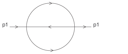
Figure 1: Sunset diagram

First we write the momentum representation of the graph:

$$G=\mathop{\displaystyle\int}\frac{d^{D}q_{1}}{i\pi^{D/2}}\frac{d^{D}q_{2}}{i\pi^{D/2}}\frac{1}{(B_{1}^{2}-m_{1}^{2})}\frac{1}{(B_{2}^{2}-m_{2}^{2})}\frac{1}{(B_{3}^{2}-m_{3}^{2})}\;,$$ (50)

where the branch momenta $B_{j}$ are in this case defined as:

$$\begin{array}[]{ll}B_{1}=&q_{1}\\ B_{2}=&q_{1}+q_{2}\\ B_{3}=&p_{1}+q_{2}.\end{array}$$ (51)

Applying Feynman parametrization we obtain the following integral:

$$G=\Gamma(3)\int\limits_{0}^{1}dx_{1}dx_{2}dx_{3}\,\delta(1-x_{1}-x_{2}-x_{3})\mathop{\displaystyle\int}\frac{d^{D}q_{1}}{i\pi^{D/2}}\frac{d^{D}q_{2}}{i\pi^{D/2}}\frac{1}{\Omega^{3}},$$ (52)

where we define

$$\Omega=\mathop{\textstyle\sum}\limits_{j=1}^{3}x_{j}B_{j}^{2}-\mathop{\textstyle\sum}\limits_{j=1}^{3}x_{j}m_{j}^{2}.$$ (53)

Then, expanding the previous sum and factorizing the result in terms of internal momenta, we get a quadratic form in these momenta, which reads:

$$\Omega=(x_{1}+x_{2})q_{1}^{2}+2x_{2}\,q_{1}.q_{2}+\left(x_{2}+x_{3}\right)q_{2}^{2}+2x_{3}\,p_{1}.q_{2}+x_{3}p_{1}^{2}-\mathop{\textstyle\sum}\limits_{j=1}^{3}x_{j}m_{j}^{2}.$$ (54)

4.1.1 Usual method of finding the parametric representation

According to the previous formulation (see equation $\left(\ref{h}\right)$), we can identify the necessary basic elements for finding the parametric representation. These are:

$$\begin{array}[]{l}\mathbf{A}=\left(\begin{array}[]{cc}x_{1}+x_{2}&x_{2}\\ x_{2}&x_{2}+x_{3}\end{array}\right)\\ \\ \mathbf{k}=\left(\begin{array}[]{cc}0&-x_{3}\,p_{1}\end{array}\right)^{t}\\ \\ J=x_{3}\,p_{1}^{2}.\end{array}$$ (55)

We start from the general result that we found in equation $\left(\ref{t}\right)$ for Feynman’s parametrization:

$$G=\dfrac{(-1)^{N_{\nu}}\Gamma(N_{\nu}-\frac{LD}{2})}{\Gamma(\nu_{1})...\Gamma(\nu_{N})}\mathop{\displaystyle\int}d\overrightarrow{x}\;\delta(1-\mathop{\textstyle\sum}\limits_{j=1}^{N}x_{j})\frac{\left[\det\mathbf{A}\right]^{N_{\nu}-(L+1)\frac{D}{2}}}{\left[\det\mathbf{A}\left(\mathop{\textstyle\sum}\limits_{j=1}^{N}x_{j}m_{j}^{2}-J+\mathbf{k}^{t}\mathbf{A}^{-1}\mathbf{k}\right)\right]^{N_{\nu}-L\frac{D}{2}}}.$$ (56)

In the present case this gives:

$$G=(-1)^{3}\Gamma(3-D)\mathop{\displaystyle\int}dx_{1}...dx_{3}\,\delta(1-\mathop{\textstyle\sum}\limits_{j=1}^{3}x_{j})\frac{\left[\det\mathbf{A}\right]^{3-3\frac{D}{2}}}{\left[\det\mathbf{A}\left(\mathop{\textstyle\sum}\limits_{j=1}^{N}x_{j}m_{j}^{2}-J+\mathbf{k}^{t}\mathbf{A}^{-1}\mathbf{k}\right)\right]^{3-D}}.$$ (57)

Evaluating the terms that are involved here we get:

$$\begin{array}[]{l}\det\mathbf{A=}x_{1}x_{2}+x_{1}x_{3}+x_{2}x_{3}\\ \mathbf{A}^{-1}=\dfrac{1}{x_{1}x_{2}+x_{1}x_{3}+x_{2}x_{3}}\left(\begin{array}[]{cc}x_{1}+x_{2}&-x_{2}\\ -x_{2}&x_{2}+x_{3}\end{array}\right)\\ \\ \mathbf{k}^{t}\mathbf{A}^{-1}\mathbf{k=}\dfrac{x_{3}^{2}(x_{1}+x_{2})p_{1}^{2}}{x_{1}x_{2}+x_{1}x_{3}+x_{2}x_{3}}\\ \\ \det\mathbf{A}\left(-J+\mathbf{k}^{t}\mathbf{A}^{-1}\mathbf{k}\right)\mathbf{=-}\left(x_{1}x_{2}x_{3}\right)p_{1}^{2}\end{array}$$ (58)

and considering also the fact that $D=4-2\epsilon$ one finally obtains the Feynman parametric representation:

$$G=-\Gamma(-1+2\epsilon)\mathop{\displaystyle\int}\limits_{0}^{1}d\overrightarrow{x}\;\delta(1-\mathop{\textstyle\sum}\nolimits_{j=1}^{3}x_{j})\dfrac{\left[x_{1}x_{2}+x_{1}x_{3}+x_{2}x_{3}\right]^{-3+3\epsilon}}{\left[\left(x_{1}x_{2}+x_{1}x_{3}+x_{2}x_{3}\right)\mathop{\textstyle\sum}\limits_{j=1}^{3}x_{j}m_{j}^{2}-\left(x_{1}x_{2}x_{3}\right)p_{1}^{2}\right]^{-1+2\epsilon}},$$ (59)

with $d\overrightarrow{x}=dx_{1}dx_{2}dx_{3}$.

4.1.2 Obtaining the scalar representation by recursion

Remembering the general formula that is used in this method for the parametric representation:

$$G=\frac{\left(-1\right)^{N_{\nu}}\Gamma(N_{\nu}-\frac{LD}{2})}{\Gamma(\nu_{1})...\Gamma(\nu_{N})}\mathop{\displaystyle\int}d\overrightarrow{x}\;\delta(1-\mathop{\textstyle\sum}\nolimits_{j=1}^{N}x_{j})\frac{\left[M_{11}^{\left(1\right)}...M_{LL}^{\left(L\right)}\right]^{\frac{-D}{2}}}{\left[\mathop{\textstyle\sum}\limits_{j=1}^{N}x_{j}m_{j}^{2}-\mathop{\textstyle\sum}\limits_{i,j=1}^{E}M_{\left(L+i\right)\left(L+j\right)}^{\left(L+1\right)}\,p_{i}.p_{j}\right]^{N_{\nu}-\frac{LD}{2}}},$$ (60)

which in the present case gets reduced to the following:

$$G=-\Gamma(-1+2\epsilon)\mathop{\displaystyle\int}dx_{1}dx_{2}dx_{3}\;\delta(1-\mathop{\textstyle\sum}\limits_{j=1}^{3}x_{j})\frac{\left[M_{11}^{\left(1\right)}M_{22}^{\left(2\right)}\right]^{-2+\epsilon}}{\left[\mathop{\textstyle\sum}\limits_{j=1}^{3}x_{j}m_{j}^{2}-M_{33}^{\left(3\right)}\,p^{2}\right]^{-1+2\epsilon}}.$$ (61)

From equation $\left(\ref{z}\right)$ one can find immediately the Initial Parameters Matrix (IPM):

$$\mathbf{M}^{(1)}=\mathbf{M}=\left(\begin{array}[]{ccc}x_{1}+x_{2}&x_{2}&0\\ x_{2}&x_{2}+x_{3}&x_{3}\\ 0&x_{3}&x_{3}\end{array}\right).$$ (62)

It is now only necessary to calculate the matrix elements using the recursive function described in section 3. Basically we need to evaluate the following identities:

$$M_{11}^{\left(1\right)} = R(M,1,1,1)$$ (63)

$$M_{22}^{\left(2\right)} = R(M,2,2,2)$$

$$M_{33}^{\left(3\right)} = R(M,3,3,3).$$

The results, after writing the commands in Maple, are respectively:

$>$R(M,1,1,1) ;

$$x_{1}+x_{2}$$

$>$R(M,2,2,2) ;

$$\frac{x_{1}x_{2}+x_{1}x_{3}+x_{2}x_{3}}{x_{1}+x_{2}}$$

$>$R(M,3,3,3) ;

$$\frac{x_{1}x_{2}x_{3}}{x_{1}x_{2}+x_{1}x_{3}+x_{2}x_{3}}$$

Thus replacing these expressions into equation $\left(\ref{u}\right)$, we obtain:

$$G=-\Gamma(-1+2\epsilon)\mathop{\displaystyle\int}d\overrightarrow{x}\;\delta(1-\mathop{\textstyle\sum}\nolimits_{j=1}^{3}x_{j})\frac{\left[x_{1}x_{2}+x_{1}x_{3}+x_{2}x_{3}\right]^{-2+\epsilon}}{\left[\mathop{\textstyle\sum}\limits_{j=1}^{3}x_{j}m_{j}^{2}-\dfrac{x_{1}x_{2}x_{3}}{x_{1}x_{2}+x_{1}x_{3}+x_{2}x_{3}}\,p^{2}\right]^{-1+2\epsilon}},$$ (64)

and then we have the same scalar representation as found before in $\left(\ref{v}\right)$:

$$G=-\Gamma(-1+2\epsilon)\mathop{\displaystyle\int}d\overrightarrow{x}\;\delta(1-\mathop{\textstyle\sum}\nolimits_{j=1}^{3}x_{j})\frac{\left[x_{1}x_{2}+x_{1}x_{3}+x_{2}x_{3}\right]^{-3+3\epsilon}}{\left[\left(x_{1}x_{2}+x_{1}x_{3}+x_{2}x_{3}\right)\mathop{\textstyle\sum}\limits_{j=1}^{3}x_{j}m_{j}^{2}-x_{1}x_{2}x_{3}\,p^{2}\right]^{-1+2\epsilon}}.$$ (65)

4.2 Example II

Let us consider now the following diagram:

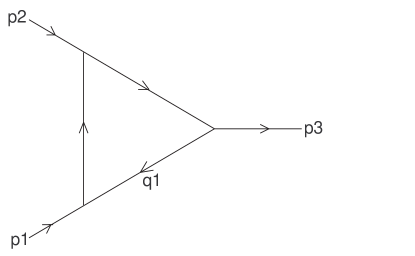
Figure 2: Triangle diagram

The loop integral is given in this case by:

$$G=\mathop{\displaystyle\int}\frac{d^{D}q_{1}}{i\pi^{D/2}}\frac{1}{(B_{1}^{2}-m_{1}^{2})}\frac{1}{(B_{2}^{2}-m_{2}^{2})}\frac{1}{(B_{3}^{2}-m_{3}^{2})},$$ (66)

where the branch momenta $B_{j}$ have been defined in the following way:

$$\begin{array}[]{l}\begin{array}[]{l}B_{1}=q_{1}\\ B_{2}=p_{1}+q_{1}\\ B_{3}=p_{1}+p_{2}+q_{1}.\end{array}\end{array}$$ (67)

The next step is to apply Feynman’s parametrization, obtaining the following integral:

$$G=\Gamma(3)\int\limits_{0}^{1}dx_{1}dx_{2}dx_{3}\,\delta(1-\mathop{\textstyle\sum}\nolimits_{j=1}^{3}x_{j})\mathop{\displaystyle\int}\frac{d^{D}q_{1}}{i\pi^{D/2}}\frac{1}{\Omega^{3}},$$ (68)

where the denominator $\Omega$ is given in terms of the internal momenta by:

$$\begin{array}[]{ll}\Omega&=\left(x_{1}+x_{2}+x_{3}\right)q_{1}^{2}+2\left[(x_{2}+x_{3})p_{1}+x_{3}\,p_{2}\right].q_{1}+\left(x_{2}+x_{3}\right)p_{1}^{2}+2x_{3}\,p_{1}.p_{2}+\\ &x_{3}\,p_{2}^{2}-\mathop{\textstyle\sum}\nolimits_{j=1}^{3}x_{j}m_{j}^{2}.\end{array}$$ (69)

4.2.1 Usual method of finding the parametric representation

Starting from equation $\left(\ref{w}\right)$ we can recognize right away the basic necessary elements for finding the parametric representation. These are:

$$\begin{array}[]{l}\mathbf{A}=\left(x_{1}+x_{2}+x_{3}\right)\\ \\ \mathbf{k}=-(x_{2}+x_{3})p_{1}-x_{3}p_{2}\\ \\ J=\left(x_{2}+x_{3}\right)p_{1}^{2}+2x_{3}p_{1}.p_{2}+x_{3}p_{2}^{2},\end{array}$$ (70)

and therefore the resulting scalar integral will be given in this case by the expression:

$$G=(-1)^{3}\Gamma(3-\frac{D}{2})\mathop{\displaystyle\int}dx_{1}...dx_{3}\;\delta(1-\mathop{\textstyle\sum}\limits_{j=1}^{3}x_{j})\frac{\left[\det\mathbf{A}\right]^{3-D}}{\left[\det\mathbf{A}\left(\mathop{\textstyle\sum}\limits_{j=1}^{N}x_{j}m_{j}^{2}-J+\mathbf{k}^{t}\mathbf{A}^{-1}\mathbf{k}\right)\right]^{3-\frac{D}{2}}}.$$ (71)

Evaluating each term, we obtain:

$$\begin{array}[]{ll}\det\mathbf{A}&\mathbf{=}x_{1}+x_{2}+x_{3}\\ \mathbf{A}^{-1}&=\dfrac{1}{x_{1}+x_{2}+x_{3}}\\ \mathbf{k}^{t}\mathbf{A}^{-1}\mathbf{k}&\mathbf{=}\dfrac{\left[(x_{2}+x_{3})p_{1}+x_{3}p_{2}\right]^{2}}{x_{1}+x_{2}+x_{3}}\end{array}$$ (72)

and

$$\begin{array}[]{ll}\det\mathbf{A}\left(-J+\mathbf{k}^{t}\mathbf{A}^{-1}\mathbf{k}\right)&\mathbf{=-(}x_{1}x_{2}+x_{1}x_{3})p_{1}^{2}-2x_{1}x_{3}p_{1}.p_{2}-\left(x_{1}x_{3}+x_{2}x_{3}\right)p_{2}^{2}\\ &\mathbf{=-}x_{1}x_{2}p_{1}^{2}-x_{2}x_{3}p_{2}^{2}-x_{1}x_{3}(p_{1}+p_{2})^{2}\\ &\mathbf{=-}x_{1}x_{2}p_{1}^{2}-x_{2}x_{3}p_{2}^{2}-x_{1}x_{3}p_{3}^{2},\end{array}$$ (73)

where we have used the condition $\left(p_{1}+p_{2}\right)^{2}=p_{3}^{2}$, and then put $D=4-2\epsilon$. Thus we finally arrive at Feynman’s parametric representation:

$$G=-\Gamma(1+\epsilon)\mathop{\displaystyle\int}\limits_{0}^{1}d\overrightarrow{x}\;\delta(1-\mathop{\textstyle\sum}\limits_{j=1}^{3}x_{j})\dfrac{\left[x_{1}+x_{2}+x_{3}\right]^{-1+2\epsilon}}{\left[\left(x_{1}+x_{2}+x_{3}\right)\mathop{\textstyle\sum}\limits_{j=1}^{3}x_{j}m_{j}^{2}-\mathbf{(}x_{1}x_{2})p_{1}^{2}-(x_{2}x_{3})p_{2}^{2}-(x_{1}x_{3})p_{3}^{2}\right]^{1+\epsilon}},$$ (74)

with $d\overrightarrow{x}=dx_{1}dx_{2}dx_{3}$.

4.2.2 Obtaining the scalar representation by recursion

In this method the general formula for the parametric representation is:

$$G=\frac{\left(-1\right)^{N_{\nu}}\Gamma(N_{\nu}-\frac{LD}{2})}{\Gamma(\nu_{1})...\Gamma(\nu_{N})}\mathop{\displaystyle\int}d\overrightarrow{x}\;\delta(1-\mathop{\textstyle\sum}\limits_{j=1}^{N}x_{j})\frac{\left[M_{11}^{\left(1\right)}...M_{LL}^{\left(L\right)}\right]^{\frac{-D}{2}}}{\left[\mathop{\textstyle\sum}\limits_{j=1}^{N}x_{j}m_{j}^{2}-\mathop{\textstyle\sum}\limits_{i,j=1}^{E}M_{\left(L+i\right)\left(L+j\right)}^{\left(L+1\right)}\,p_{i}.p_{j}\right]^{N_{\nu}-\frac{LD}{2}}},$$ (75)

which in our case is reduced to the following in $D=4-2\epsilon$ dimensions:

$$G=-\Gamma(1+\epsilon)\mathop{\displaystyle\int}dx_{1}dx_{2}dx_{3}\;\delta(1-\mathop{\textstyle\sum}\limits_{j=1}^{3}x_{j})\frac{\left[M_{11}^{\left(1\right)}\right]^{-2+\epsilon}}{\left[\mathop{\textstyle\sum}\limits_{j=1}^{3}x_{j}m_{j}^{2}-M_{22}^{\left(2\right)}\,p_{1}^{2}-M_{23}^{\left(2\right)}p_{1}.p_{2}-M_{32}^{\left(2\right)}p_{2}.p_{1}-M_{33}^{\left(2\right)}p_{2}^{2}\right]^{1+\epsilon}}.$$ (76)

The next step consists in the evaluation of the matrix elements of $M_{ij}^{\left(k\right)}$. In order to do this, and starting from equation $\left(\ref{w}\right)$ we find the Initial Parameters Matrix ( MPI):

$$\mathbf{M}^{(1)}=\mathbf{M}=\left(\begin{array}[]{ccc}x_{1}+x_{2}+x_{3}&x_{2}+x_{3}&x_{3}\\ x_{2}+x_{3}&x_{2}+x_{3}&x_{3}\\ x_{3}&x_{3}&x_{3}\end{array}\right).$$ (77)

Using the recursive routine proposed in section 3, the necessary matrix elements $M_{ij}^{\left(k\right)}$ are evaluated:

$$\begin{array}[]{l}M_{11}^{\left(1\right)}=R(M,1,1,1)\\ M_{22}^{\left(2\right)}=R(M,2,2,2)\\ M_{23}^{\left(2\right)}=M_{32}^{\left(2\right)}=R(M,2,2,3)\\ M_{33}^{\left(2\right)}=R(M,2,2,2),\end{array}$$ (78)

and executing the Maple commands, we get the following results:

$>$R(M,1,1,1) ;

$$x_{1}+x_{2}+x_{3}$$

$>$R(M,2,2,2) ;

$$\frac{x_{1}x_{2}+x_{1}x_{3}}{x_{1}+x_{2}+x_{3}}$$

$>$R(M,2,2,3) ;

$$\frac{x_{1}x_{3}}{x_{1}+x_{2}+x_{3}}$$

$>$R(M,2,3,3) ;

$$\frac{x_{1}x_{3}+x_{2}x_{3}}{x_{1}+x_{2}+x_{3}}.$$

For the sum $\mathop{\textstyle\sum}\nolimits_{i,j=1}^{2}M_{\left(L+i\right)\left(L+j\right)}^{\left(L+1\right)}\,p_{i}.p_{j}$, we get:

$$\begin{array}[]{ll}\mathop{\textstyle\sum}\limits_{i,j=1}^{2}M_{\left(L+i\right)\left(L+j\right)}^{\left(L+1\right)}\,p_{i}.p_{j}&=\dfrac{\left(x_{1}x_{2}+x_{1}x_{3}\right)p_{1}^{2}+2x_{1}x_{3}\,p_{1}.p_{2}+\left(x_{1}x_{3}+x_{2}x_{3}\right)p_{2}^{2}}{x_{1}+x_{2}+x_{3}}\\ &=\dfrac{\left(x_{1}x_{2}\right)p_{1}^{2}+\left(x_{2}x_{3}\right)p_{2}^{2}+\left(x_{1}x_{3}\right)p_{3}^{2}}{x_{1}+x_{2}+x_{3}}.\end{array}$$ (79)

Thus, replacing these quantities in $\left(\ref{y}\right)$, we obtain:

$$G=-\Gamma(1+\epsilon)\mathop{\displaystyle\int}dx_{1}dx_{2}dx_{3}\;\delta(1-\mathop{\textstyle\sum}\limits_{j=1}^{3}x_{j})\frac{\left[x_{1}+x_{2}+x_{3}\right]^{-2+\epsilon}}{\left[\mathop{\textstyle\sum}\limits_{j=1}^{3}x_{j}m_{j}^{2}-\dfrac{\left(x_{1}x_{2}\right)p_{1}^{2}+\left(x_{2}x_{3}\right)p_{2}^{2}+\left(x_{1}x_{3}\right)p_{3}^{2}}{x_{1}+x_{2}+x_{3}}\right]^{1+\epsilon}},$$ (80)

which finally is reduced to the same parametric representation deduced before in $\left(\ref{x}\right)$:

$$G=-\Gamma(1+\epsilon)\mathop{\displaystyle\int}d\overrightarrow{x}\;\delta(1-\mathop{\textstyle\sum}\limits_{j=1}^{3}x_{j})\frac{\left[x_{1}+x_{2}+x_{3}\right]^{-1+2\epsilon}}{\left[\left(x_{1}+x_{2}+x_{3}\right)\mathop{\textstyle\sum}\limits_{j=1}^{3}x_{j}m_{j}^{2}-\left(x_{1}x_{2}\right)p_{1}^{2}-\left(x_{2}x_{3}\right)p_{2}^{2}-\left(x_{1}x_{3}\right)p_{3}^{2}\right]^{1+\epsilon}},$$ (81)

where $d\overrightarrow{x}=dx_{1}dx_{2}dx_{3}$.

5
Summary :

5.1 Usual Parametric Representation

$$A=\left(\begin{array}[]{lll}a_{11}&\ldots&a_{1L}\\ \vdots&&\quad\vdots\\ a_{L1}&\ldots&a_{LL}\end{array}\right)$$

$$\mathbf{q}=\left[q_{1}\,q_{2}\,...q_{L}\right]^{t}\Longrightarrow\text{Only internal momenta.}$$

$$\Downarrow$$

FEYNMAN PARAMETRIZATION

Before

$$\framebox{$G=\dfrac{\Gamma(N_{\nu})}{\Gamma(\nu_{1})...\Gamma(\nu_{N})}\int\limits_{0}^{1}d\overrightarrow{x}\,\delta(1-\mathop{\textstyle\sum}\limits_{j=1}^{N}x_{j})\mathop{\displaystyle\int}\dfrac{\mathop{\textstyle\prod}\limits_{j=1}^{L}d^{D}q_{j}}{\left(i\pi^{D/2}\right)^{L}}\dfrac{1}{\left[\mathbf{q}^{t}\mathbf{Aq}-2\mathbf{k}^{t}\mathbf{q}+J-\mathop{\textstyle\sum}\limits_{j=1}^{N}x_{j}m_{j}^{2}\right]^{N_{\nu}}}$}$$

After

$$\framebox{$G=\dfrac{\left(-1\right)^{N_{\nu}}\Gamma(N_{\nu}-\frac{LD}{2})}{\Gamma(\nu_{1})...\Gamma(\nu_{N})}\mathop{\displaystyle\int}\limits_{0}^{1}d\overrightarrow{x}\;\delta(1-\mathop{\textstyle\sum}\limits_{j=1}^{N}x_{j})\dfrac{\left[\det\mathbf{A}\right]^{N_{\nu}-(L+1)\frac{D}{2}}}{\left[\det\mathbf{A}\left(\mathop{\textstyle\sum}\limits_{j=1}^{N}x_{j}m_{j}^{2}-J+\mathbf{k}^{t}\mathbf{A}^{-1}\mathbf{k}\right)\right]^{\left(N_{\nu}-\frac{LD}{2}\right)}}$}$$

SCHWINGER PARAMETRIZATION

Before

$$\framebox{$G=\dfrac{1}{\Gamma(\nu_{1})...\Gamma(\nu_{N})}\mathop{\displaystyle\int}\limits_{0}^{\infty}d\overrightarrow{x}\exp\left(\mathop{\textstyle\sum}\limits_{j=1}^{N}x_{j}m_{j}^{2}-J\right)\mathop{\displaystyle\int}\dfrac{\mathop{\textstyle\prod}\limits_{j=1}^{L}d^{D}q_{j}}{\left(i\pi^{D/2}\right)^{L}}\exp\left(-\mathbf{q}^{t}\mathbf{Aq+}2\mathbf{k}^{t}\mathbf{q}\right)$}$$

After

$$G=\dfrac{(-1)^{\frac{LD}{2}}}{\Gamma(\nu_{1})...\Gamma(\nu_{N})}\mathop{\displaystyle\int}\limits_{0}^{\infty}d\overrightarrow{x} \left[\det\mathbf{A}\right]^{-\frac{D}{2}}\exp\left(\mathop{\textstyle\sum}\limits_{j=1}^{N}x_{j}m_{j}^{2}-J+\mathbf{k}^{t}\mathbf{A}^{-1}\mathbf{k}\right)$$ 

5.2 Alternative Parametric Representation Form in terms of the matrix elements $M_{ij}^{(k)}$

$$M^{\left(1\right)}=\left(\begin{array}[]{ll}\begin{array}[]{lll}a_{11}&\ldots&a_{1L}\\ \vdots&&\quad\vdots\\ a_{L1}&\ldots&a_{LL}\end{array}&\begin{array}[]{lll}&\ldots&M_{{}_{1\left(L+E\right)}}^{(1)}\\ &&\\ &&\qquad\vdots\end{array}\\ \begin{array}[]{lll}&&\\ \vdots&&\\ M_{\left({}_{L+E}\right)1}^{(1)}&&\ldots\end{array}&\begin{array}[]{lll}\ddots&&\\ &&\\ &&M_{{}_{\left(L+E\right)\left(L+E\right)}}^{(1)}\end{array}\end{array}\right)$$

$$\mathbf{Q}=\left[q_{1}\,q_{2}\,...q_{L\,}\,p_{1}\,p_{2\,}...p_{E}\right]\Longrightarrow\text{Internal and external momenta.}$$

$$\Downarrow$$

FEYNMAN PARAMETRIZATION

Before

$$\framebox{$G=\dfrac{\Gamma(N_{\nu})}{\Gamma(\nu_{1})...\Gamma(\nu_{N})}\mathop{\displaystyle\int}\limits_{0}^{1}d\overrightarrow{x}\,\delta(1-\mathop{\textstyle\sum}\limits_{j=1}^{N}x_{j})\mathop{\displaystyle\int}\dfrac{\mathop{\textstyle\prod}\limits_{j=1}^{L}d^{D}Q_{j}}{i\pi^{D/2}}\dfrac{1}{\left[\mathbf{Q}^{t}M^{\left(1\right)}\mathbf{Q}-\mathop{\textstyle\sum}\limits_{j=1}^{N}x_{j}m_{j}^{2}\right]^{N_{\nu}}}$}$$

After

$$\framebox{$G=\dfrac{\left(-1\right)^{N_{\nu}}\Gamma(N_{\nu}-\frac{LD}{2})}{\Gamma(\nu_{1})...\Gamma(\nu_{N})}\mathop{\displaystyle\int}\limits_{0}^{1}d\overrightarrow{x}\;\delta(1-\mathop{\textstyle\sum}\limits_{j=1}^{N}x_{j})\dfrac{\left[M_{11}^{\left(1\right)}...M_{LL}^{\left(L\right)}\right]^{\frac{-D}{2}}}{\left[\mathop{\textstyle\sum}\limits_{j=1}^{N}x_{j}m_{j}^{2}-\mathop{\textstyle\sum}\limits_{i,j=1}^{E}M_{\left(L+i\right)\left(L+j\right)}^{\left(L+1\right)}\,p_{i}.p_{j}\right]^{N_{\nu}-\frac{LD}{2}}}$}$$

SCHWINGER PARAMETRIZATION

Before

$$\framebox{$G=\dfrac{1}{\Gamma(\nu_{1})...\Gamma(\nu_{N})}\mathop{\displaystyle\int}\limits_{0}^{\infty}d\overrightarrow{x}\exp\left(\mathop{\textstyle\sum}\limits_{j=1}^{N}x_{j}m_{j}^{2}\right)\mathop{\displaystyle\int}\dfrac{\mathop{\textstyle\prod}\limits_{j=1}^{L}d^{D}Q_{j}}{\left(i\pi^{D/2}\right)^{L}}\exp\left(-\mathop{\textstyle\sum}\limits_{j=1}^{N}\mathbf{Q}^{t}\mathbf{M}^{\left(1\right)}\mathbf{Q}\right)$}$$

After

$$G=\dfrac{(-1)^{\frac{LD}{2}}}{\Gamma(\nu_{1})...\Gamma(\nu_{N})}\mathop{\displaystyle\int}\limits_{0}^{\infty}d\overrightarrow{x} \left[M_{11}^{\left(1\right)}...M_{LL}^{\left(L\right)}\right]^{-\frac{D}{2}}\exp\left(\mathop{\textstyle\sum}\limits_{j=1}^{N}x_{j}m_{j}^{2}-\mathop{\textstyle\sum}\limits_{i,j=1}^{E}M_{\left(L+i\right)\left(L+j\right)}^{\left(L+1\right)}\,p_{i}.p_{j}\right)$$ 

5.3 Alternative Parametric Representation Form in terms of subdeterminants of the MPI

FEYNMAN PARAMETRIZATION

Before

$$\framebox{$G=\dfrac{\Gamma(N_{\nu})}{\Gamma(\nu_{1})...\Gamma(\nu_{N})}\mathop{\displaystyle\int}\limits_{0}^{1}d\overrightarrow{x}\,\delta(1-\mathop{\textstyle\sum}\limits_{j=1}^{N}x_{j})\mathop{\displaystyle\int}\dfrac{\mathop{\textstyle\prod}\limits_{j=1}^{L}d^{D}Q_{j}}{i\pi^{D/2}}\dfrac{1}{\left[\mathbf{Q}^{t}M^{\left(1\right)}\mathbf{Q}-\mathop{\textstyle\sum}\limits_{j=1}^{N}x_{j}m_{j}^{2}\right]^{N_{\nu}}}$}$$

After

$$\framebox{$G=\dfrac{\left(-1\right)^{N_{\nu}}\Gamma(N_{\nu}-\frac{LD}{2})}{\Gamma(\nu_{1})...\Gamma(\nu_{N})}\mathop{\displaystyle\int}\limits_{0}^{1}d\overrightarrow{x}\;\delta(1-\mathop{\textstyle\sum}\limits_{j=1}^{N}x_{j})\dfrac{\left[\Delta_{LL}^{(L)}\right]^{N_{\nu}-(L+1)\frac{D}{2}}}{\left[\Delta_{LL}^{(L)}\mathop{\textstyle\sum}\limits_{j=1}^{N}x_{j}m_{j}^{2}-\mathop{\textstyle\sum}\limits_{i,j=1}^{E}\Delta_{(L+i)(L+j)}^{(L+1)}\,p_{i}.p_{j}\right]^{N_{\nu}-\frac{LD}{2}}}$}$$

SCHWINGER PARAMETRIZATION

Before

$$\framebox{$G=\dfrac{1}{\Gamma(\nu_{1})...\Gamma(\nu_{N})}\mathop{\displaystyle\int}\limits_{0}^{\infty}d\overrightarrow{x}\exp\left(\mathop{\textstyle\sum}\limits_{j=1}^{N}x_{j}m_{j}^{2}\right)\mathop{\displaystyle\int}\dfrac{\mathop{\textstyle\prod}\limits_{j=1}^{L}d^{D}Q_{j}}{\left(i\pi^{D/2}\right)^{L}}\exp\left(-\mathop{\textstyle\sum}\limits_{j=1}^{N}\mathbf{Q}^{t}\mathbf{M}^{\left(1\right)}\mathbf{Q}\right)$}$$

After

$$\framebox{$G=\dfrac{(-1)^{\frac{LD}{2}}}{\Gamma(\nu_{1})...\Gamma(\nu_{N})}\mathop{\displaystyle\int}\limits_{0}^{\infty}d\overrightarrow{x}\,\left[\Delta_{LL}^{(L)}\right]^{-\frac{D}{2}}\exp\left(\dfrac{\Delta_{LL}^{(L)}\mathop{\textstyle\sum}\limits_{j=1}^{N}x_{j}m_{j}^{2}-\mathop{\textstyle\sum}\limits_{i,j=1}^{E}\Delta_{(L+i)(L+j)}^{(L+1)}\,p_{i}.p_{j}}{\Delta_{LL}^{(L)}}\right)$}$$

6 Conclusions

There are two main aspects that need to be emphasized in the present work. The first is the simplicity of the method, both in the actual calculation and in its application to a particular topology. From the point of view of the mathematical structure of the final scalar representation, there is a remarkable difference with the usual method. In the usual parametric form of a loop integral, it is necessary to evaluate a scalar term and a matrix product that involves an inverse matrix calculation. The method proposed in this work is based on a simple change in the initial procedure in the search for a parametric representation of the momentum integral, so that both the scalar term and the matrix product with inverse matrix are included in an expansion of internal products of external momenta, in which the coefficients of such expansion are determinants of submatrices of the matrix that relates internal and external momenta (IPM). The evaluation of determinants is much simpler than the evaluation of matrix inverses. Moreover, the most important aspect is that such determinants can be in turn calculated from matrix elements obtained using a recursion relation starting from the IPM, in a simple and straightforward way.

The second relevant aspect is that this method can be easily implemented computationally. This allows for a fast automatization of Feynman diagram generation, obtaining simply and directly the parametric representation as a step towards a complete numerical or analytical evaluation whenever possible.

7 Bibliography

APPENDICES

Appendix A Quadratic Forms and its diagonalization by square completion

A quadratic form in $n$ variables is an expression which can be written in matrix form as the product $\mathbf{x}^{t}\mathbf{Mx}$, where $\mathbf{x}$ is an n-dimensional vector, given by $\mathbf{x}=\left[x_{1},...,x_{n}\right]^{t}$, and $\mathbf{M}$ is a generic $n\times n$ dimensional matrix. That is:

$$\mathbf{x}^{t}\mathbf{Mx}=\mathop{\textstyle\sum}\limits_{i=1}^{n}\mathop{\textstyle\sum}\limits_{j=1}^{n}x_{i}M_{ij}x_{j}.$$ (82)

Let $\mathbf{D}$ be an $n\times n$ diagonal matrix. The expressions $\mathbf{\ x}^{t}\mathbf{Mx}$ and $\overline{\mathbf{y}}^{t}\mathbf{Dy}$ are equivalent if there exists a linear transformation $\mathbf{y}=\mathbf{Px}$ and $\overline{\mathbf{y}}=\overline{\mathbf{P}}\mathbf{x}$ such that $\mathbf{x}^{t}\mathbf{Mx}=\overline{\mathbf{y}}^{t}\mathbf{Dy}$, that is:

$$\mathbf{M}=\overline{\mathbf{P}}^{t}\mathbf{DP.}$$ (83)

The quadratic form is then transformed into a sum of $n$ linear terms of the type $\overline{y}_{i}y_{j}\delta_{ij}.$

A.1 Square Completion Procedure

A.1.1 Completing the square for $x_{1}$

Every Quadratic Form can be diagonalized using the square completion procedure, which generates the required linear transformation. First we define a matrix $\mathbf{M}=\mathbf{M}^{\left(1\right)}$, and then we expand the matrix product $\mathbf{x}^{t}\mathbf{M}^{\left(1\right)}\mathbf{x}$ in order to complete the square associated to the parameter $x_{1}$. Then we arrive at the following result:

$$\begin{array}[]{ll}\mathbf{x}^{t}\mathbf{M}^{\left(1\right)}\mathbf{x}&=\mathop{\textstyle\sum}\limits_{i=1}^{n}\mathop{\textstyle\sum}\limits_{j=1}^{n}x_{i}M_{ij}^{(1)}x_{j}\\ &=M_{11}^{\left(1\right)}x_{1}^{2}+x_{1}\left(\mathop{\textstyle\sum}\limits_{j=2}^{n}M_{1j}^{\left(1\right)}x_{j}\right)+\left(\mathop{\textstyle\sum}\limits_{i=2}^{n}x_{i}M_{i1}^{\left(1\right)}\right)x_{1}+\mathop{\textstyle\sum}\limits_{i,j=2}^{n}x_{i}M_{ij}^{\left(1\right)}x_{j}\\ &=M_{11}^{\left(1\right)}\left[x_{1}^{2}+x_{1}\left(\mathop{\textstyle\sum}\limits_{j=2}^{n}\dfrac{M_{1j}^{\left(1\right)}}{M_{11}^{\left(1\right)}}x_{j}\right)+\left(\mathop{\textstyle\sum}\limits_{i=2}^{n}x_{i}\dfrac{M_{i1}^{\left(1\right)}}{M_{11}^{\left(1\right)}}\right)x_{1}\right]+\mathop{\textstyle\sum}\limits_{i,j=2}^{n}x_{i}M_{ij}^{\left(1\right)}x_{j}\\ &=M_{11}^{\left(1\right)}\left[\left(x_{1}+\mathop{\textstyle\sum}\limits_{i=2}^{n}x_{i}\dfrac{M_{i1}^{\left(1\right)}}{M_{11}^{\left(1\right)}}\right)\left(x_{1}+\mathop{\textstyle\sum}\limits_{j=2}^{n}\dfrac{M_{1j}^{\left(1\right)}}{M_{11}^{\left(1\right)}}x_{j}\right)\right]+\mathop{\textstyle\sum}\limits_{i,j=2}^{n}x_{i}\left(M_{ij}^{\left(1\right)}-\dfrac{M_{i1}^{\left(1\right)}M_{1j}^{\left(1\right)}}{M_{11}^{\left(1\right)}}\right)x_{j}.\end{array}$$ (84)

Let us define now the new variables:

$$\begin{array}[]{ccc}\overline{y}_{1}&=&x_{1}+\mathop{\displaystyle\sum}\limits_{i=2}^{n}x_{i}\dfrac{M_{i1}^{\left(1\right)}}{M_{11}^{\left(1\right)}}\\ y_{1}&=&x_{1}+\mathop{\displaystyle\sum}\limits_{j=2}^{n}\dfrac{M_{1j}^{\left(1\right)}}{M_{11}^{\left(1\right)}}x_{j},\end{array}$$ (85)

and also the matrix $\mathbf{M}^{\left(2\right)}=\left\{M_{ij}^{\left(2\right)}\right\}$, such that the elements of this be given by the relation:

$$\begin{array}[]{c}M_{ij}^{\left(2\right)}=M_{ij}^{\left(1\right)}-\dfrac{M_{i1}^{\left(1\right)}M_{1j}^{\left(1\right)}}{M_{11}^{\left(1\right)}}.\end{array}$$ (86)

Therefore we can rewrite the quadratic form $\left(\ref{aa}\right)$, with the first parameter already diagonalized, in the following way:

$$\mathbf{x}^{t}\mathbf{M}^{\left(1\right)}\mathbf{x}=M_{11}^{\left(1\right)}\overline{y}_{1}y_{1}+\mathop{\textstyle\sum}\limits_{i=2}^{n}\mathop{\textstyle\sum}\limits_{j=2}^{n}x_{i}M_{ij}^{\left(2\right)}x_{j}.$$ (87)

The second term in the right hand side can be simplified, since from the equation $\left(\ref{1}\right)$ one obtains that $M_{j1}^{\left(2\right)}=M_{1j}^{\left(2\right)}=0$, for $1\leq j\leq n$. Thus we can write:

$$\mathop{\textstyle\sum}\limits_{i=2}^{n}\mathop{\textstyle\sum}\limits_{j=2}^{n}x_{i}M_{ij}^{\left(2\right)}x_{j}=\mathop{\textstyle\sum}\limits_{i=1}^{n}\mathop{\textstyle\sum}\limits_{j=1}^{n}x_{i}M_{ij}^{\left(2\right)}x_{j}=\mathbf{x}^{t}\mathbf{M}^{\left(2\right)}\mathbf{x.}$$ (88)

In summary, in the quadratic expansion the first term has been already diagonalized, a fact that can be described by the following expression:

$$\mathbf{x}^{t}\mathbf{M}^{\left(1\right)}\mathbf{x}=M_{11}^{\left(1\right)}\overline{y}_{1}y_{1}+\mathbf{x}^{t}\mathbf{M}^{\left(2\right)}\mathbf{x.}$$ (89)

A.1.2 Completing the square for $x_{2}$

Now we take the second term of $\left(\ref{2}\right)$, and the same procedure followed above is repeated in order to complete the square for the parameter $x_{2}$, which gives:

$$\begin{array}[]{ll}\mathbf{x}^{t}\mathbf{M}^{\left(2\right)}\mathbf{x}&=\mathop{\textstyle\sum}\limits_{i=2}^{n}\mathop{\textstyle\sum}\limits_{j=2}^{n}x_{i}M_{ij}^{\left(2\right)}x_{j}\\ &=M_{22}^{\left(2\right)}x_{2}^{2}+x_{2}\left(\mathop{\textstyle\sum}\limits_{j=3}^{n}M_{2j}^{\left(2\right)}x_{j}\right)+\left(\mathop{\textstyle\sum}\limits_{i=3}^{n}x_{i}M_{i2}^{\left(2\right)}\right)x_{2}+\mathop{\textstyle\sum}\limits_{i,j=3}^{n}x_{i}M_{ij}^{\left(2\right)}x_{j}\\ &=M_{22}^{\left(2\right)}\left[\left(x_{2}+\mathop{\textstyle\sum}\limits_{i=3}^{n}x_{i}\dfrac{M_{i2}^{\left(2\right)}}{M_{22}^{\left(2\right)}}\right)\left(x_{2}+\mathop{\textstyle\sum}\limits_{j=3}^{n}\dfrac{M_{2j}^{\left(2\right)}}{M_{22}^{\left(2\right)}}x_{j}\right)\right]+\mathop{\textstyle\sum}\limits_{i,j=3}^{n}x_{i}\left(M_{ij}^{\left(2\right)}-\dfrac{M_{i2}^{\left(2\right)}M_{2j}^{\left(2\right)}}{M_{22}^{\left(2\right)}}\right)x_{j}.\end{array}$$ (90)

Let us define, analogously to equation $\left(\ref{3}\right)$, the new variables:

$$\begin{array}[]{ccc}\overline{y}_{2}&=&x_{2}+\mathop{\textstyle\sum}\limits_{i=3}^{n}x_{i}\frac{M_{i2}^{\left(2\right)}}{M_{22}^{\left(2\right)}}\\ y_{2}&=&x_{2}+\mathop{\textstyle\sum}\limits_{j=3}^{n}\frac{M_{2j}^{\left(2\right)}}{M_{22}^{\left(2\right)}}x_{j},\end{array}$$ (91)

and the matrix $\mathbf{M}^{\left(3\right)}=\left\{M_{ij}^{\left(3\right)}\right\}$,   where we set $M_{ij}^{\left(3\right)}=M_{ij}^{\left(2\right)}-\dfrac{M_{i2}^{\left(2\right)}M_{2j}^{\left(2\right)}}{M_{22}^{\left(2\right)}}$. Then we obtain:

$$\mathbf{x}^{t}\mathbf{M}^{\left(2\right)}\mathbf{x}=M_{22}^{\left(2\right)}\overline{y_{2}}y_{2}+\mathop{\textstyle\sum}\limits_{i=3}^{n}\mathop{\textstyle\sum}\limits_{j=3}^{n}x_{i}M_{ij}^{\left(3\right)}x_{j}.$$ (92)

The expression for the matrix element $M_{ij}^{\left(3\right)}$ implies that $M_{2j}^{\left(3\right)}=M_{j2}^{\left(3\right)}=0$, with $2\leq j\leq n$, and since we also had that $M_{1j}^{\left(2\right)}=M_{j1}^{\left(2\right)}=0$, then $M_{1j}^{\left(3\right)}=M_{j1}^{\left(3\right)}=0$, where $1\leq j\leq n$. In this way we can write the second term as:

$$\mathop{\textstyle\sum}\limits_{i=3}^{n}\mathop{\textstyle\sum}\limits_{j=3}^{n}x_{i}M_{ij}^{\left(3\right)}x_{j}=\mathop{\textstyle\sum}\limits_{i=1}^{n}\mathop{\textstyle\sum}\limits_{j=1}^{n}x_{i}M_{ij}^{\left(3\right)}x_{j}=\mathbf{x}^{t}\mathbf{M}^{\left(3\right)}\mathbf{x},$$ (93)

and therefore now the first two components of $\mathbf{x}$ have been diagonalized:

$$\mathbf{x}^{t}\mathbf{M}^{\left(1\right)}\mathbf{x}=M_{11}^{\left(1\right)}\overline{y}_{1}y_{1}+M_{22}^{\left(2\right)}\overline{y}_{2}y_{1}+\mathbf{x}^{t}\mathbf{M}^{\left(3\right)}\mathbf{x.}$$ (94)

A.1.3 Generalization of the Square Completion Procedure for $x_{j}$

Notice that the last term in $\left(\ref{5}\right)$ is another quadratic form, which then will allow us to complete the square for the parameter $x_{3}$. The procedure can be repeated successively for $x_{3},...,x_{n}$, and therefore the following relations are determined by induction:

$$\begin{array}[]{l}\overline{y}_{l}=x_{l}+\mathop{\textstyle\sum}\nolimits_{i=l+1}^{n}x_{i}\dfrac{M_{il}^{\left(l\right)}}{M_{ll}^{\left(l\right)}}\\ y_{l}=x_{l}+\mathop{\textstyle\sum}\nolimits_{j=l+1}^{n}\dfrac{M_{lj}^{\left(l\right)}}{M_{ll}^{\left(l\right)}}x_{j}\\ M_{ij}^{\left(l+1\right)}=\left\{\begin{tabular}[]{l}$0$ \ \ \ \ \ \ \ \ \ \ \ \ \ \ \ \ \ \ \ \ \ \ \ , if $\ i<(l+1)$ $\ \vee$ $\ j<(l+1)$\\ $M_{ij}^{\left(l\right)}-\dfrac{M_{il}^{\left(l\right)}M_{lj}^{\left(l\right)}}{M_{ll}^{\left(l\right)}}$ \ \ , in other cases.\end{tabular}\right.\end{array}$$ (95)

Here the matrix $\mathbf{M}^{(k)}$ (con $1\leq k\leq n$) has the following generic structure:

$$\mathbf{M}^{(k)}=\left(\begin{array}[]{llllll}0&&\cdots&&&\quad 0\\ &&&&&\quad\vdots\\ \vdots&&0&\cdots&&\quad 0\\ &&\vdots&M_{kk}^{(k)}&\cdots&M_{kn}^{(k)}\\ &&&\vdots&&\quad\vdots\\ 0&\cdots&0&M_{nk}^{(k)}&\cdots&M_{nn}^{(k)}\end{array}\right).$$ (96)

In general, the procedure of square completion of the k-element of $\mathbf{x}$, for $1\leq k<n$, transforms the initial quadratic form into:

$$\mathbf{x}^{t}\mathbf{M}^{\left(1\right)}\mathbf{x}=M_{11}^{\left(1\right)}\overline{y}_{1}y_{1}+...+M_{kk}^{\left(k\right)}\overline{y}_{k}y_{k}+\mathbf{x}^{t}\mathbf{M}^{\left(k+1\right)}\mathbf{x.}$$ (97)

The complete process, that is after $n$ square completions, diagonalizes the quadratic form $\mathbf{x}^{t}\mathbf{M}^{\left(1\right)}\mathbf{x}$ and transforms it into a diagonal bilineal structure, of the form:

$$\mathbf{x}^{t}\mathbf{M}^{\left(1\right)}\mathbf{x}=M_{11}^{\left(1\right)}\overline{y}_{1}y_{1}+...+M_{nn}^{\left(n\right)}\overline{y}_{n}y_{n}=\overline{\mathbf{y}}^{t}\mathbf{Dy},$$ (98)

where we identify:

$$\begin{array}[]{l}D=diag\left[M_{11}^{\left(1\right)},M_{22}^{\left(2\right)},...,M_{nn}^{\left(n\right)}\right]\\ \overline{\mathbf{y}}=\left[\overline{y}_{1},...,\overline{y}_{n}\right]^{t}\\ \mathbf{y}=\left[y_{1},...,y_{n}\right]^{t}.\end{array}$$ (99)

A.2 Some Properties

1. The relation between the vectors $\overline{y},y$ and $x$, is defined by the equation $\left(\ref{4}\right)$, and from it we can identify the transformation matrices that fulfill the equations:

   $$\mathbf{y}=\mathbf{Px}\quad\wedge\quad\overline{\mathbf{y}}=\overline{\mathbf{P}}\mathbf{x}.$$ (100)

   Specifically it is possible to determine $\mathbf{P}$ and $\overline{\mathbf{P}}$, given by:

   $$P=\left(\begin{array}[]{ccccc}1&\frac{M_{12}^{\left(1\right)}}{M_{11}^{\left(1\right)}}&\frac{M_{13}^{\left(1\right)}}{M_{11}^{\left(1\right)}}&\cdots&\frac{M_{1n}^{\left(1\right)}}{M_{11}^{\left(1\right)}}\\ 0&1&\frac{M_{23}^{\left(1\right)}}{M_{22}^{\left(2\right)}}&\cdots&\frac{M_{2n}^{\left(2\right)}}{M_{22}^{\left(2\right)}}\\ \vdots&0&1&&\vdots\\ &&\ddots&\ddots&\\ 0&\cdots&&0&1\end{array}\right)$$ (101)

   $$\overline{P}=\left(\begin{array}[]{lllll}1&\frac{M_{21}^{\left(1\right)}}{M_{11}^{\left(1\right)}}&\frac{M_{31}^{\left(1\right)}}{M_{11}^{\left(1\right)}}&\cdots&\frac{M_{n1}^{\left(1\right)}}{M_{11}^{\left(1\right)}}\\ 0&1&\frac{M_{32}^{\left(2\right)}}{M_{22}^{\left(2\right)}}&\cdots&\frac{M_{n2}^{\left(2\right)}}{M_{22}^{\left(2\right)}}\\ \vdots&0&1&&\vdots\\ &&\ddots&\ddots&\\ 0&\cdots&&0&1\end{array}\right)$$ (102)

2. From the equations in $\left(\ref{4}\right)$, we find that:

   $$\begin{array}[]{l}\overline{y}_{n}=y_{n}=x_{n}\\ \mathbf{M}^{(n+1)}=\left\{0\right\}\end{array}$$ (103)

3. The transformation matrices $\mathbf{P}$ and $\overline{\mathbf{P}}$ have the following property:

   $$\begin{array}[]{c}\det\mathbf{P}=\det\mathbf{P}^{t}=1\\ \det\overline{\mathbf{P}}=\det\overline{\mathbf{P}}^{t}=1\end{array}$$ (104)

4. If $\mathbf{M}^{(1)}=\left[\mathbf{M}^{(1)}\right]^{t}$ (symmetric case), then the following identities hold:

$$\begin{array}[]{l}\overline{\mathbf{y}}=\mathbf{y}\\ \overline{\mathbf{P}}=\mathbf{P}\\ \mathbf{M}^{(k)}=\left[\mathbf{M}^{(k)}\right]^{t}\\ \mathbf{x}^{t}\mathbf{M}^{(1)}\mathbf{x}=\mathbf{y}^{t}\mathbf{Dy}\\ \mathbf{M}^{(1)}=\mathbf{P}^{t}\mathbf{DP},\end{array}$$ (105)

where the matrix $\mathbf{D}$ is the diagonal matrix given by:

$$\mathbf{D}=diag\left[M_{11}^{\left(1\right)},M_{22}^{\left(2\right)},...,M_{nn}^{\left(n\right)}\right].$$ (106)

A.3 Evaluation of the determinant of $\mathbf{M}^{\left(1\right)}$

From the previous results, the determinant of $\mathbf{M}^{\left(1\right)}$ is given by:

$$\det\mathbf{M}^{(1)}=\det\overline{\mathbf{P}}^{t}\mathbf{DP}=\det\overline{\mathbf{P}}^{t}.\det\mathbf{D}.\det\mathbf{P}=M_{11}^{\left(1\right)}M_{22}^{\left(2\right)}...M_{nn}^{\left(n\right)}.$$ (107)

The conditions for evaluating this determinant are given in Appendix B.

Appendix B Matrices $\mathbf{M}^{(k)}$

B.1 Generalization of the matrices $\mathbf{M}^{(k)}$

It is possible to generalize the $n\times n$ dimensional matrices $\mathbf{M}^{(k)}$ starting from the recurrence equation:

$$M_{ij}^{(k+1)}=M_{ij}^{(k)}-\frac{M_{ik}^{(k)}M_{kj}^{(k)}}{M_{kk}^{(k)}}.$$ (108)

As an example let us consider a generic matrix $\mathbf{A}_{n\times n}=\left\{a_{ij}\right\}$, and define an input matrix $\mathbf{M}^{(1)}\equiv\mathbf{A}_{n\times n}$.

B.1.1 Generating $\mathbf{M}^{(2)}$

Let us evaluate the particular cases of the first row and first column. That is:

$$M_{1j}^{(2)}=M_{1j}^{(1)}-\frac{M_{11}^{(1)}M_{1j}^{(1)}}{M_{11}^{(1)}}=0,\qquad(j=1,..,n)$$ (109)

$$M_{i1}^{(2)}=M_{i1}^{(1)}-\frac{M_{i1}^{(1)}M_{11}^{(1)}}{M_{11}^{(1)}}=0,\qquad(i=1,..,n).$$ (110)

The other matrix elements do not present a particular interest, and are evaluated using the recursion relation $(\ref{6})$. Then the matrix $\mathbf{M}^{(2)}$ gets structured in the following manner:

$$\mathbf{M}^{(2)}=\left(\begin{array}[]{cccc}0&\cdots&&0\\ \vdots&M_{22}^{(2)}&\cdots&M_{2n}^{(2)}\\ &\vdots&&\vdots\\ 0&M_{n2}^{(2)}&\cdots&M_{nn}^{(2)}.\end{array}\right).$$ (111)

Notice that $\mathbf{M}^{(2)}$ is computable only if $M_{11}^{(1)}\neq 0$.

B.1.2 Generating $\mathbf{M}^{(3)}$

Having $\mathbf{M}^{(2)}$ already evaluated one can construct $\mathbf{M}^{(3)}$. Let us analyze the first and second row. For the first row we have that:

$$M_{1j}^{(3)}=M_{1j}^{(2)}-\frac{M_{12}^{(2)}M_{2j}^{(2)}}{M_{22}^{(2)}}=0,\qquad\text{since }M_{1j}^{(2)}=0.\text{ \qquad}(j=1,...,n),$$ (112)

while for the second row:

$$M_{2j}^{(3)}=M_{2j}^{(2)}-\frac{M_{22}^{(2)}M_{2j}^{(2)}}{M_{22}^{(2)}}=0.$$ (113)

Analogously, for the first and second column we have the following values respectively:

$$M_{i1}^{(3)}=M_{i1}^{(2)}-\frac{M_{i2}^{(2)}M_{21}^{(2)}}{M_{22}^{(2)}}=0,\qquad\text{since }M_{i1}^{(2)}=0\text{ \qquad}(i=1,...,n)$$ (114)

and

$$M_{i2}^{(3)}=M_{i2}^{(2)}-\frac{M_{i2}^{(2)}M_{22}^{(2)}}{M_{22}^{(2)}}=0.$$ (115)

The other elements have values according to $(\ref{6})$. Finally the matrix  $\mathbf{M}^{(3)}$ gets the following form:

$$\mathbf{M}^{(3)}=\left(\begin{array}[]{ccccc}0&\cdots&&\cdots&0\\ \vdots&0&\cdots&&0\\ &\vdots&M_{33}^{(3)}&\cdots&M_{3n}^{(3)}\\ \vdots&&\vdots&&\vdots\\ 0&0&M_{n3}^{(3)}&\cdots&M_{nn}^{(3)}.\end{array}\right).$$ (116)

The matrix is defined only if the matrix element $M_{22}^{(2)}\neq 0$. The procedure can be repeated successively for the rest of the matrices generated by recursion, thus finding that for $k\in[1,...,n]$ one gets:

$$\mathbf{M}^{(k)}=\left(\begin{array}[]{cccccc}0&\cdots&&&\cdots&0\\ \vdots&&&&&\vdots\\ &&0&\cdots&&0\\ &&\vdots&M_{kk}^{(k)}&\cdots&M_{kn}^{(k)}\\ \vdots&&&\vdots&&\vdots\\ 0&\cdots&0&M_{kn}^{(k)}&\cdots&M_{nn}^{(k)},\end{array}\right)$$ (117)

with the condition that $\mathbf{M}^{(k)}$ is defined only if $M_{kk}^{(k)}\neq 0$ or $k=1,2,...,n-1$.

B.2 Elements $M_{ij}^{(k)}$

From the previous results we van find the relation that exists between the matrix elements generated by recursion and the input matrix elements $\mathbf{M}^{(1)}=\mathbf{A}_{n\times n}=\{a_{ij}\}$. For $M_{ij}^{(2)}$

$$M_{ij}^{(2)}=M_{ij}^{(1)}-\frac{M_{i1}^{(1)}M_{1j}^{(1)}}{M_{11}^{(1)}}=\frac{M_{11}^{(1)}M_{ij}^{(1)}-M_{i1}^{(1)}M_{i1}^{(1)}}{M_{11}^{(1)}}=\frac{\left|\begin{array}[]{cc}M_{11}^{(1)}&M_{i1}^{(1)}\\ M_{i1}^{(1)}&M_{ij}^{(1)}\end{array}\right|}{\left|M_{11}^{(1)}\right|}$$ (118)

o equivalently

$$M_{ij}^{(2)}=\frac{\left|\begin{array}[]{cc}a_{11}&a_{1j}\\ a_{i1}&a_{ij}\end{array}\right|}{\left|a_{11}\right|}.$$ (119)

For $M_{ij}^{(3)}$ we have that:

$$M_{ij}^{(3)}=M_{ij}^{(2)}-\tfrac{M_{i2}^{(2)}M_{2j}^{(2)}}{M_{22}^{(2)}}=\frac{\left|\begin{array}[]{cc}a_{11}&a_{1j}\\ a_{i1}&a_{ij}\end{array}\right|}{\left|a_{11}\right|}-\frac{\left|\begin{array}[]{cc}a_{11}&a_{12}\\ a_{i1}&a_{i2}\end{array}\right|\left|\begin{array}[]{cc}a_{11}&a_{1j}\\ a_{21}&a_{2j}\end{array}\right|}{\left|a_{11}\right|\left|\begin{array}[]{cc}a_{11}&a_{12}\\ a_{21}&a_{22}\end{array}\right|}.$$ (120)

Some simple algebra gives the following result:

$$M_{ij}^{(3)}=\frac{\left|\begin{array}[]{ccc}a_{11}&a_{12}&a_{1j}\\ a_{21}&a_{22}&a_{2j}\\ a_{i1}&a_{i2}&a_{ij}\end{array}\right|}{\left|\begin{array}[]{cc}a_{11}&a_{12}\\ a_{21}&a_{22}\end{array}\right|}.$$ (121)

Let us now define the determinant $\Delta_{ij}^{(k+1)}$, such that it corresponds to the determinant of a submatrix of the input matrix $\mathbf{M}^{(1)}=\mathbf{A}_{n\times n}$, whose dimension is $(k+1)\times(k+1)$, and which is given by the following identity:

$$\Delta_{ij}^{(k+1)}=\left|\begin{array}[]{cccc}a_{11}&\cdots&a_{1k}&a_{1j}\\ \vdots&&\vdots&\vdots\\ a_{k1}&\cdots&a_{kk}&a_{kj}\\ a_{i1}&\cdots&a_{ik}&a_{ij}\end{array}\right|.$$ (122)

Let us see the following examples:

B.2.1 Example I

$$\Delta_{34}^{(2)}=\left|\begin{array}[]{cc}a_{11}&a_{14}\\ a_{41}&a_{34}\end{array}\right|.$$ (123)

B.2.2 Example II

$$\Delta_{33}^{(3)}=\left|\begin{array}[]{ccc}a_{11}&a_{12}&a_{13}\\ a_{21}&a_{22}&a_{23}\\ a_{31}&a_{32}&a_{33}\end{array}\right|.$$ (124)

Applying this definition in the equations $(\ref{7})$ and $(\ref{8})$, we obtain:

$$M_{ij}^{(2)}=\frac{\Delta_{ij}^{(2)}}{\Delta_{11}^{(1)}},$$ (125)

$$M_{ij}^{(3)}=\frac{\Delta_{ij}^{(3)}}{\Delta_{22}^{(2)}}.$$ (126)

Through an induction process we can directly generalize the relation that exists between the matrix elements of $M_{ij}^{(k)}$ and the input matrix $\mathbf{M}^{(1)}=\mathbf{A}_{n\times n}$. In general one gets:

$$\mathbf{M}_{ij}^{(k+1)}=\dfrac{\Delta_{ij}^{(k+1)}}{\Delta_{kk}^{(k)}}.$$ (127)

B.3 The matrix $\mathbf{M}^{(k)}$ in terms of determinants of submatrices of $\ \mathbf{M}^{(1)}$

In appendix A it was previously shown that the determinant of the input matrix $\mathbf{M}^{(1)}=\mathbf{A}_{n\times n}$ is given by the expression:

$$\det\mathbf{A}=\det\mathbf{M}^{(1)}=M_{11}^{(1)}M_{22}^{(2)}...M_{nn}^{(n)}.$$ (128)

Using equation $(\ref{9})$ we can write the matrix elements $M_{kk}^{(k)}$ as ratios of determinants of submatrices of $\mathbf{M}^{(1)}$. Then we have that:

$$\det\mathbf{A}_{n\times n}=\det\mathbf{M}^{(1)}=\dfrac{\Delta_{11}^{(1)}}{\Delta_{00}^{(0)}}\dfrac{\Delta_{22}^{(2)}}{\Delta_{11}^{(1)}}...\dfrac{\Delta_{(n-1)(n-1)}^{(n-1)}}{\Delta_{(n-2)(n-2)}^{(n-2)}}\dfrac{\Delta_{nn}^{(n)}}{\Delta_{(n-1)(n-1)}^{(n-1)}}=\dfrac{\Delta_{nn}^{(n)}}{\Delta_{00}^{(0)}}.$$ (129)

Here $\Delta_{00}^{(0)}=1$, which can be shown by calculating the determinant of a scalar. Let us evaluate the determinant of the matrix $\mathbf{M}^{\left(1\right)}=\mathbf{A}_{1\mathbf{\times}1}=\left(a_{11}\right)$, that is:

$$\det\mathbf{A}_{1\mathbf{\times}1}=\mathbf{\det M}^{\left(1\right)}=a_{11}.$$

On the other hand we have that:

$$\det\mathbf{A}_{1\mathbf{\times}1}=\mathbf{\det M}^{\left(1\right)}=M_{11}^{(1)}=\frac{\bigtriangleup_{11}^{\left(1\right)}}{\bigtriangleup_{00}^{\left(0\right)}},$$ (130)

and applying equation $(\ref{10})$ one obtains that $\bigtriangleup_{11}^{\left(1\right)}=a_{11}$, which by comparison gives:

$$\bigtriangleup_{00}^{\left(0\right)}=1.$$ (131)

Finally it is shown that:

$$\det\mathbf{A}_{\mathbf{n\times n}}=\det\mathbf{M}^{(1)}=\Delta_{nn}^{(n)}=\left|\begin{array}[]{ccc}a_{11}&\cdots&a_{1n}\\ \vdots&&\vdots\\ a_{n1}&\cdots&a_{nn}\end{array}\right|,$$ (132)

a result that is evidently correct. In summary we can rewrite the matrix $\mathbf{M}^{(k)}$ in terms of subdeterminants of $\mathbf{M}^{(1)}=\mathbf{A}_{\mathbf{n}\times\mathbf{n}}$, that is:

$$\mathbf{M}^{(k)}=\dfrac{1}{\Delta_{(k-1)(k-1)}^{(k-1)}}\left(\begin{array}[]{cccccc}0&\cdots&&&\cdots&0\\ \vdots&&&&&\vdots\\ &&0&\cdots&&0\\ &&\vdots&\Delta_{kk}^{(k)}&\cdots&\Delta_{kn}^{(k)}\\ \vdots&&&\vdots&&\vdots\\ 0&\cdots&0&\Delta_{nk}^{(k)}&\cdots&\Delta_{nn}^{(k)}.\end{array}\right).$$ (133)

Notice that the relation of the recursive matrix elements with the ratios of determinants provides the condition for evaluating the matrix $\mathbf{M}^{(k)}$. This is that the determinants $\Delta_{(k-1)(k-1)}^{(k-1)}$(Principal Minors) be non-vanishing, a condition that is evident in identity $(\ref{11})$.

B.4 Evaluation of determinants $\Delta_{ij}^{\left(l\right)}$ in terms of the matrix elements of $\mathbf{M}^{(k)}$

The relation that we found for the recursive matrix elements in terms of a ratio of determinants is given by the equation:

$$M_{ij}^{(k+1)}=\dfrac{\Delta_{ij}^{(k+1)}}{\Delta_{kk}^{(k)}}.$$ (134)

We can reorder this such that:

$$\Delta_{ij}^{(k+1)}=\Delta_{kk}^{(k)}M_{ij}^{(k+1)},$$ (135)

where $\Delta_{kk}^{(k)}$ corresponds to a determinant called the Principal Minor of order $k\times k$, which can be expressed directly in terms of recursive matrix elements, such that:

$$\Delta_{kk}^{(k)}=M_{11}^{(1)}...M_{kk}^{(k)}$$ (136)

and therefore we obtain the identity:

$$\Delta_{ij}^{(k+1)}=M_{11}^{(1)}...M_{kk}^{(k)}M_{ij}^{(k+1)},$$

which allows for the possibility of evaluating any subdeterminant of the matrix $\mathbf{M}^{(1)}$.

References

- [1] C. Itzykson, J. Zuber, Quantum Fields Theory, World Scientific, Singapore, 1993.
- [2] M. Le Bellac, Quantum and Statistical Field Theory, University Press, New York, 1991.
- [3] M. E. Peskin, D. V. Schroeder, An Introduction to Quantum Field Theory, Perseus, Reading, MA, 1995.
- [4] W. Greiner, S. Schramm, E. Stein, Quantum Chromodynamics, Springer, Berlin, 2002.
- [5] V. A. Smirnov, Evaluating Feynman Integrals, Springer, Berlin, Heidelberg, 2004; and references therein.
- [6] T. Binoth, G. Heinrich, Nucl. Phys. B 585 (2000) 741, hep-ph/0004013.
- [7] T. Binoth, G. Heinrich, Nucl. Phys. B 680 (2004) 375, hep-ph/0305234.
- [8] N. Nakanishi, Graph Theory and Feynman Integrals, Gordon and Breach, New York, 1971.
- [9] K. Hoffman, R. Kunze, Álgebra Lineal, Prentice Hall, Mexico,1973.
- [10] H. Anton, Introducción al Álgebra Lineal, Limusa, Mexico DF, 1998.
- [11] R. Barbolla, P.Sanz, Álgebra Lineal y Teoría de Matrices, Prentice Hall, Madrid, 1998.