Normalization anomalies in level truncation calculations

Abstract:

We test oscillator level truncation regularization in string field theory by calculating descent relations among vertices, or equivalently, the overlap of wedge states. We repeat the calculation using bosonic, as well as fermionic ghosts, where in the bosonic case we do the calculation both in the discrete and in the continuous basis. We also calculate analogous expressions in field level truncation. Each calculation gives a different result. We point out to the source of these differences and in the bosonic ghost case we pinpoint the origin of the difference between the discrete and continuous basis calculations. The conclusion is that level truncation regularization cannot be trusted in calculations involving normalization of singular states, such as wedge states, rank-one squeezed state projectors and string vertices.

1 Introduction

The number of fields in string field theory [1] is infinite. In string theory the infinite number of fields is of great importance for the natural renormalizability of the theory. In string field theory the infinite number of fields is a source for both conceptual and technical challenges. Level truncation offers a practical solution for the technical problems, but has no bearing on the conceptual side, for the simple reason that there is no proof that level truncation is a consistent regularization.

There are several different level truncation schemes. In field level truncation [2] the level refers to the field’s total level, and fields above a certain level are ignored. In oscillator level truncation, oscillators up to a certain level are used and all possible fields generated by these operators are considered.

Field level truncation was much used in the study of tachyon condensation. The tachyon potential should be background independent [3]. Thus, it is enough to focus on the universal subspace generated by the matter Virasoro generators and by the $b,c$ ghosts [4, 5]. The (physical) universal subspace of ghost number one can be generated by matter and ghost Virasoro generators. In this context the tachyon vacuum was evaluated to a remarkable accuracy [6]. Field level truncation was also used to study other problems, such as spontenuos Lorentz and CPT breaking [7].

The calculation of D-brane tension ratio in vacuum string field theory is an example for the use of oscillator level truncation [8]. Taylor suggested using oscillator level truncation as a way to calculate perturbative diagrams in string field theory [9]. Oscillator level truncation is the main subject of this paper and is what we mean by level truncation unless stated otherwise. We also address field level truncation in the universal basis, though to a more limited extent.

The use of level truncation may be problematic in light of the fact that it does not respect the Virasoro symmetry, especially in calculations that involve infinities that should be somehow regularized. In field theory the primary test for a regularization scheme is that it respects the symmetries involved. It was demonstrated in various contexts that similar considerations should hold in string field theory [10, 11, 12].

In order to avoid the potential problems of level truncation, one can try to use the method of diagonalizing the infinite-size matrices involved in the definition of the star product. The zero-momentum matter vertex was diagonalized in [13]. Following this work, the vertex including the zero mode and the ghost sector was diagonalized in [14, 15, 16, 17]. The diagonal form of the vertex drastically simplifies calculations, at least for some star-subalgebras [18, 19]. It also carries the promise of getting analytical results in string field theory [20, 11]. However, an anomaly in descent relations and wedge state inner products in the diagonal basis was found in [17, 21, 22]. An interesting interpretation of this anomaly was given in [23]. Here, we re-examine this anomaly and relate it to an anomaly in the level truncation calculation.

Our testing ground for level truncation is the $\left<\vphantom{V_{1}}{V_{3}}\right|\left.\!\vphantom{V_{3}}{V_{1}}\right>$ descent relation. String vertices describe string interactions by gluing, with the $N$-vertex $\left<V_{N}\right|$ gluing $N$ string fields, according to,

$${\vphantom{\left<V_{N}\right|}}_{N..1}\!\left<V_{N}\right|\left|\Psi_{1}\right>_{1}..\left|\Psi_{N}\right>_{N}=\int\Psi_{1}\star..\star\Psi_{N}\,,$$ (1)

where the star product and integral implement the gluing [1]. Since string vertices can be considered as states in multi-string spaces, they can be glued by other vertices. This fact induces the following descent relations among the string vertices,

$${\vphantom{\left<V_{n}\right|}}_{1..n}\!\left<V_{n}\right|{\vphantom{\left<V_{m}\right|}}_{(n+1)..(n+m)}\!\left<V_{m}\right|\left|V_{2}\right>_{1,(n+m)}={\vphantom{\left<V_{n+m-2}\right|}}_{2..(n+m-1)}\!\left<V_{n+m-2}\right|\,.$$ (2)

The normalization constant of this relation for $n=3,m=1$ is what was found to be anomalous when evaluated using bosonized ghosts in the continuous basis. It was not clear whether the source of the anomaly is the level truncation, the use of bosonic ghosts or the use of the continuous basis. The relation of the continuous basis to level truncation lies in the fact that divergent quantities are regularized by relating them to $\log\ell$, where $\ell$ is the truncation level.

In this paper, we repeat the calculation in the discrete basis for both bosonic and fermionic ghosts. The results we get are different from the previous calculations, but still anomalous. For the bosonic ghost, we discuss these differences in section 2 and show explicitly how the calculation in the discrete basis can be modified to give the result of the continuous basis. In section 3 we perform the fermionic ghost calculation and get a new value for the anomaly. We believe that the reason for the discrepancy between the bosonic and fermionic ghost calculations is the non-linear relation between them, $b,c=:e^{\pm\rho}:$.

In light of the success of level truncation calculations, in particular those of [9], our claim of an anomaly needs an explanation. In [9], Taylor had to integrate over a parameter $T$, representing the length of an intermediate string. The limit $T\rightarrow 0$ corresponds to calculating the descent relation $\left<V_{3}\right|\left<V_{3}\right|\left|V_{2}\right>=\left<V_{4}\right|$. This is a singular limit of the integrands in [9], but the singularity is integrable. The calculation at $T=0$ is anomalous, but it does not contribute to the integral.

Another discrepancy with [9] lies in the form of the fits. For arbitrary expression $X$, we use fits of the form $X=a+b/\ell^{c}$, where $\ell$ is the level and $a,b,c$ are parameters, while in [9], $c=1$ always gives good fits. The fact that our values for $c$ are not too far from unity (they are in the range 0.2 .. 2.0), together with the observation in [9] that convergence becomes slower as $T=0$ is approached, resolve this issue. The value of $c$ was studied in a related context in [24].

An alternative description of the anomaly is in terms of inner product of specific wedge states [5]. Wedge states are surface states [25, 26], and as such are described as exponentials of Virasoro generators over particular vacua. Wedge states are also easy to deal with since they are diagonal in the continuous basis [13]. However, the continuous basis representation can be regarded as a generic source of singularity for diagonal states, since their defining matrix is proportional to $\delta({\kappa}-{\kappa}^{\prime})$. This is the origin of anomalies in this case.

Field level truncation is natural for describing surface states and wedge states in particular. In section 4, we suggest that anomalies are possible in this description as well, despite the fact that we cannot trace them in the level truncation using Virasoro generators with vanishing central carge, $c=0$. To that end we use field level truncation with Virasoro generators of arbitrary $c$. We also compare these calculations to the analogous ones in the matter sector using oscillator level truncation and continuous basis techniques. We conclude in section 5 by summarizing our results and suggesting future research directions.

2 Bosonic ghost

In this section we calculate the descent relations using the bosonic ghost. We start by setting our conventions in 2.1, then we evaluate the normalization in 2.2. There is no “simple” way to calculate the normalization. We perform the calculation in the discrete and in the continuous basis using level truncation. In the continuous basis, level truncation manifests itself by regulating infinities using expressions that are proportional to $\log\ell$. In both calculations the “infinite” contributions cancel each other, but the final result is anomalous, with different results in each calculation. We end by comparing the anomalies in these two cases.

2.1 The vertices

In the matter sector the form of the vertices is,

$$\left|V_{N}(P_{0})\right>=\delta\Big{(}\sum_{i=1}^{N}p_{0}^{i}\Big{)}\exp\left(-\frac{1}{2}A^{\dagger}V_{N}A^{\dagger}+P_{0}V_{N0}A^{\dagger}-\frac{1}{2}P_{0}V_{N00}P_{0}\right)\left|0\right>_{N}\,.$$ (3)

$P_{0}$ is an $N$-vector of the zero-momenta $p_{0}^{i}$. $A^{\dagger}$ is an $N$-vector of creation operators in the $N$ Fock spaces, which also has a hidden index $n$ for the excitation number inside the Fock space. $V_{N}$ is an $N$ by $N$ matrix of infinite bi-linear forms. $V_{N0}$ is an $N$ vector of infinite vectors, $V_{N00}$ is an $N$ by $N$ matrix of scalars and $\left|0\right>_{N}$ is the direct product of $N$ Fock space vacua. To keep things simple, we are suppressing the 26 dimensional space-time indices, but it is crucial to have 26 dimensions for the cancellation of the infinite normalization.

For the identity state ($N=1$), $V_{1}$ is the twist matrix $C$, $V_{10}=0$ and $V_{100}=0$. For the two-vertex $V_{2}^{12}=V_{2}^{21}=C$, $V_{2}^{11}=V_{2}^{22}=0$, $V_{20}=0$ and $V_{200}=0$. The three-vertex is a bit more complicated. Its coefficients in the regular oscillator basis are summed up nicely in [8]. For the continuous basis, they can be found in [27].

The vertex in the bosonic ghost sector is similar, but with some modifications due to the anomalous ghost current,

$$\left|V^{g}_{N}(Q_{0})\right>=\delta_{\sum_{i=1}^{N}q_{0}^{i}-\frac{3}{2}(N-2)}\exp\left(-\frac{1}{2}A^{\dagger}V^{g}_{N}A^{\dagger}+Q_{0}V^{g}_{N0}A^{\dagger}-\frac{1}{2}Q_{0}V^{g}_{N00}Q_{0}\right)\left|0\right>_{N}.$$ (4)

$Q_{0}$ is an $N$-vector of zero-momenta $q_{0}^{i}$, which are discrete half-integer numbers. That is why the Dirac delta becomes a Kronecker delta. To describe the coefficients in the ghost sector, it is useful to introduce the vector $J$ that relates the mid-point to the zero mode,

$$X\big{(}\frac{\pi}{2}\big{)} =x_{0}+\sum_{n=1}^{\infty}J_{n}x_{n}=x_{0}+\int d{\kappa}J_{\kappa}x^{\kappa}\,,$$ (5)

$$J_{2n} =\sqrt{2}(-1)^{n}\,,\quad J_{2n+1}=0\,,$$ (6)

$$J_{\kappa} ={\cal P}\frac{\sqrt{2}}{{\kappa}\sqrt{{{\cal N}}({\kappa})}}\,,$$ (7)

where as usual,

$${\cal N}({\kappa})\equiv\frac{2}{\pi}\sinh\big{(}\frac{{\kappa}\pi}{2}\big{)}\,.$$ (8)

For the identity state, $V^{g}_{1}=V_{1}=C$, $V^{g}_{10}=\sqrt{2}J$ and $V^{g}_{100}=0$. For the two-vertex, the bosonic ghost coefficients are identical to the matter sector. This is a result of the fact that the constant term in the Kronecker delta is zero in this case. For the three-vertex $V^{g}_{3}=V_{3}$, $V^{g}_{30}=V_{30}+\frac{\sqrt{2}}{3}J$ and $V^{g}_{300}=V_{300}-\frac{3}{2}\log\left(\frac{27}{16}\right)$. One way to calculate the last constant is from the identity,

$$\left<q_{0}^{1}=-\frac{3}{2}\right|\left<q_{0}^{2}=-\frac{3}{2}\right|\left<q_{0}^{3}=\frac{3}{2}\right|\left|\vphantom{\frac{3}{2}}V_{3}\right>=1\,.$$ (9)

2.2 The anomaly

We can now use the results of [28] to calculate,

$$\left<\vphantom{V_{3}}{V_{1}}\right|\left.\!\vphantom{V_{1}}{V_{3}}\right>=\gamma_{13}\left|V_{2}\right>\,.$$ (10)

This is the first non-trivial descent relation. If we use a consistent regularization, we should get $\gamma_{13}=1$. The expression for $\gamma_{13}$ is,

$$\gamma_{13}=\det({\bf 1}-CV_{3}^{11})^{-\frac{D+1}{2}}\exp\frac{9}{4}\Bigl{(} -\frac{1}{2}V_{30}^{g11}({\bf 1}-CV_{3}^{11})^{-1}CV_{30}^{g11}+V_{10}^{g}({\bf 1}-V_{3}^{11}C)^{-1}V_{30}^{g11}$$ (11)

$$-\frac{1}{2}V_{10}^{g}({\bf 1}-V_{3}^{11}C)^{-1}V_{3}^{11}V_{10}^{g}-\frac{1}{2}V_{300}^{g11}\Bigr{)}.$$

This computation involves infinite matrices, therefore it should be consistently regularized. The two methods that we can try to deploy are level truncation in the discrete basis and regularization in the continuous basis. The two methods give different result and both results are wrong. We explain the difference between the two methods and show how the truncation in the discrete basis can be modified to give the same result as in the continuous basis.

In level truncation we did the calculation up to level 1000, giving $\gamma_{13}\approx 0.340$. This result is summarized in figure 1.

Figure 1: This plot shows the value of $\gamma_{13}$ calculated for levels from 1 to 1000. We get different behaviors for even and odd levels. This is in accord with the difference between odd and even levels described in [13]. Both cases fit nicely to a function of the form $a+b/\ell^{c}$, with a common limit value $a=0.340$, with $b=0.0948,-0.159$ and $c=1.19,0.91$ for the even and odd cases respectively. Both the calculated points and the fitted curves are plotted in this graph, but it is impossible to tell them apart. One remarkable feature of the fit is that it fits well starting from level 1.

The continuous basis calculation was performed in [27]. The strategy there was to use the identity,

$$\det(M)=\exp\big{(}\operatorname{tr}(\log\,M)\big{)}\,,$$ (12)

in order to represent the determinant in a similar way to the other part of the expression, which can also be represented using a trace. Then, in order to evaluate the trace of a matrix, which is diagonal in the continuous basis, the following identity was used,

$$\operatorname{tr}(A)=\int_{-\infty}^{\infty}d{\kappa}\,\rho({\kappa})a_{\kappa}\,.$$ (13)

Here, $A$ is such a matrix, $a_{\kappa}$ is the ${\kappa}$ eigenvalue of $A$ and $\rho({\kappa})$ is the divergent spectral density. In level truncation the spectral density is given by,

$$\rho^{\ell}({\kappa})=\frac{\log\ell}{2\pi}+\rho^{\ell}_{\text{fin}}({\kappa})\,,$$ (14)

and $\rho^{\ell}_{\text{fin}}({\kappa})$ has a finite limit for $\ell\rightarrow\infty$ [17, 21, 22],

$$\rho_{\text{fin}}({\kappa})=\frac{4\log(2)-2\gamma-\psi(1+\frac{i{\kappa}}{2})-\psi(1-\frac{i{\kappa}}{2})}{4\pi}\,.$$ (15)

Here, $\gamma$ is Euler’s constant and $\psi$ is the digamma function. In the evaluation of (11), the infinite part (the part that is proportional to $\log\ell$) dropped out in $D=26$ dimensions and the final result of the calculation was,

$$\gamma_{13}=3^{3/8}e^{\frac{3}{2}\gamma+36\zeta^{\prime}(-1)}\Big{(}\frac{\Gamma\big{(}\frac{1}{3}\big{)}}{\sqrt{\pi}}\Big{)}^{9}\approx 0.382948\,,$$ (16)

where $\zeta$ is the Zeta-function. The same result was later obtained in [23], where it was given a different interpretation.

Both methods give the wrong result, but the results are suspiciously close. There are two reasons for the difference between the two results. One difference comes from the evaluation of the determinant using (12). The calculation in the continuous basis is equivalent to truncating the matrix $\log M$ and then taking the level to infinity, while in level truncation we truncate the matrix $M$ itself. Since $(\log M)_{\ell}\neq\log(M_{\ell})$ we are getting different results. To demonstrate that this is the source of the difference, we repeat the level truncation calculation, but this time we calculate the determinant as follows,

$$(\det M)_{\ell,m}=\exp\Big{(}\operatorname{tr}\big{(}\log(M_{\ell\cdot m})_{\ell}\big{)}\Big{)},$$ (17)

where $\ell$ is the level and $m$ stands for a margin. Here, we evaluate the matrix to level $m\cdot\ell$, calculate the log of this matrix, truncate the result to level $\ell$, take the trace and then exponentiate.

Since the trace diverges, we have to add an infinity of the form $\frac{3}{2}H_{\ell/2}$, where $H$ is the harmonic number, to the result. After adding this term, the result for the trace in the ${\kappa}$ basis is $-1.7448$. For regular level truncation we get -1.8278 at level 100 and for the corrected level truncation we get $-1.7411$. These results are summarized in figure 2.

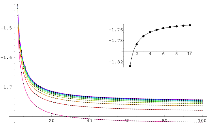
Figure 2: This graph shows the effect of the different truncation in the calculation of the determinant. The lowest plot in the spectrum has $m=1$, the next one has $m=2$ and so on up to $m=10$. The fit parameters for $a+b/\ell^{c}$ give $b$ in the range 0.624 to 0.625, $c$ in the range 0.93 to 0.94 and the sub-graph shows the ten values of $a$. The extrapolation of this graph with the same type of fit gives us the estimate of $-1.7411$ (with $b=-0.103,c=1.19$). If we ignore the first point when extrapolating the sub-graph we will get a result of $-1.7433$ and ignoring the first five points would give $-1.7449$. This demonstrates that the result of $-1.7448$ that we get in the continuous basis is within the error of the level truncation calculation.

The second difference comes from the matrix inversion in the exponent. Again, the calculation in the continuous basis is equivalent to truncating the matrix after the inversion, while in level truncation we first truncate the matrix and only then invert it. To demonstrate that this is the source of the difference, we repeat the level truncation calculation but this time we calculate the matrix to be inverted up to level $m\cdot\ell$, invert the matrix and only then truncate it to level $\ell$. This time we have to subtract $\frac{3}{2}H_{\ell/2}$ from the results in order to overcome the divergences. After this subtraction, the result in the continuous basis is $\frac{3}{2}\log\frac{27}{16}\approx 0.7849$. For the regular level truncation we get $0.7515$ and for the corrected truncation we get $0.7851$. These results are summarized in figure 3.

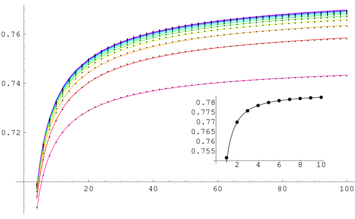
Figure 3: This graph shows the effect of the different truncation in the calculation of the exponent. The lowest plot in the spectrum has $m=1$, the next one has $m=2$ and so on up to $m=10$. The fit parameters for $a+b/\ell^{c}$ give $b$ in the range -0.15 to -0.19, $c$ in the range 0.63 to 0.59 and the sub-graph shows the ten values of the extrapolated main plots. The extrapolation of this graph gives us the estimate of $0.7851$ (with $b=-0.03,c=1.26$). If we ignore the first point when extrapolating the sub-graph we will get a result of $0.7846$ and ignoring the first five points would give $0.7843$. This demonstrates that the continuous basis result of $0.7849$ is within the error of the level truncation result.

3 Fermionic ghost

It was suspected that the mismatch in the continuous basis calculations may be the result of using the bosonized ghosts [21]. It is clear that level truncation does not commute with bosonization, which is a non-linear transformation. In this section, we verify that indeed the result of the evaluation is changed when using fermionic ghosts in the level truncation. However, the result is still not the expected value of unity. We start by setting our conventions and defining the fermionic ghost vertices. Then, we turn to the evaluation of the anomaly. We also confirm that there is no anomaly in the result other than in the normalization.

3.1 The vertices

One of the features of the ghost sector is the existence of several vacua, due to the ghost zero modes. Here, we follow the conventions of [29] by defining,

$$\left|\downarrow\right>\equiv c_{1}\left|0\right>,\qquad\left|\uparrow\right>\equiv c_{0}c_{1}\left|0\right>.$$ (18)

We also define [25],

$$\left|3\right>\equiv c_{-1}c_{0}c_{1}\left|0\right>.$$ (19)

Each vacuum has its BPZ conjugate,

$$\left<\downarrow\right|=\left<0\right|c_{-1}\,,\qquad\left<\uparrow\right|=\left<0\right|c_{-1}c_{0}\,,\qquad\left<3\right|=\left<0\right|c_{-1}c_{0}c_{1}\,.$$ (20)

We normalize the vacua in the usual way,

$$\left<\vphantom{3}{0}\right|\left.\!\vphantom{0}{3}\right>=\left<\vphantom{\uparrow}{\downarrow}\right|\left.\!\vphantom{\downarrow}{\uparrow}\right>=\left<\vphantom{\downarrow}{\uparrow}\right|\left.\!\vphantom{\uparrow}{\downarrow}\right>=\left<\vphantom{0}{3}\right|\left.\!\vphantom{3}{0}\right>=1\,.$$ (21)

Vertices of order two and higher are described using tensor products of string field spaces. In this case our conventions are,

$$\left|\Psi_{1},\Psi_{2}\right>_{12}=\left|\Psi_{1}\right>_{1}\left|\Psi_{2}\right>_{2}\,,\qquad{\vphantom{\left<\Psi_{1},\Psi_{2}\right|}}_{12}\!\left<\Psi_{1},\Psi_{2}\right|={\vphantom{\left<\Psi_{1}\right|}}_{1}\!\left<\Psi_{1}\right|{\vphantom{\left<\Psi_{2}\right|}}_{2}\!\left<\Psi_{2}\right|.$$ (22)

Higher multi-string spaces are treated similarly. For calculations that involve tensor products, we also have to define the parity of the $\operatorname{SL}(2)$ invariant vacua. We use the conventions of [1], according to which the right vacuum $\left|0\right>$ is even, while the left vacuum $\left<0\right|$ is odd, though one can also use the opposite definitions [30]. Both vacua have ghost number zero.

The ghost number of an $N$-vertex is $3(N-1)$. This follows from the definition of the $N$-vertex (1), the requirement of having three ghosts to saturate the inner product in each string field space and the fact that the string field integral is non-vanishing only for ghost number three operators. This is also consistent with the descent relations (2).

Taking the parity conventions into account, we deduce that the parity of $\left|V_{N}\right>$ is $-(-1)^{N}$, while $\left<V_{N}\right|$ is always odd. This is also consistent with (2). Our parity conventions imply the following symmetry properties for the two-string vacua,

$$\left|0\right>_{12} =\left|0\right>_{21}, \qquad\left|\downarrow\right>_{12} =-\left|\downarrow\right>_{21}, \qquad\left|\uparrow\right>_{12} =\left|\uparrow\right>_{21}, \qquad\left|3\right>_{12} =-\left|3\right>_{21},$$ (23)

$${\vphantom{\left<3\right|}}_{12}\!\left<3\right| ={\vphantom{\left<3\right|}}_{21}\!\left<3\right|, \qquad{\vphantom{\left<\uparrow\right|}}_{12}\!\left<\uparrow\right| =-{\vphantom{\left<\uparrow\right|}}_{21}\!\left<\uparrow\right|, \qquad{\vphantom{\left<\downarrow\right|}}_{12}\!\left<\downarrow\right| ={\vphantom{\left<\downarrow\right|}}_{21}\!\left<\downarrow\right|, \qquad{\vphantom{\left<0\right|}}_{12}\!\left<0\right| =-{\vphantom{\left<0\right|}}_{21}\!\left<0\right|.$$

Similar expressions hold for higher tensor products.

The one string vertex $\left<V_{1}\right|$ is the BPZ conjugate of the identity string field, which is a surface state defined by the conformal map,

$$f(z)=\frac{z}{1-z^{2}}\,.$$ (24)

The generating function and the defining matrix in the ghost sector are [25, 31],

$$S(z,w) =\frac{f^{\prime}(z)^{2}f^{\prime}(w)^{-1}}{f(z)-f(w)}\left(\frac{f(w)-f(0)}{f(z)-f(0)}\right)^{3}-\frac{1}{z-w}\left(\frac{w}{z}\right)^{3}.$$ (25)

$${(S_{0})}_{nm} =-(-1)^{n+m}\oint_{0}\frac{dzdw}{(2\pi i)^{2}}\frac{S(z,w)}{z^{m-1}w^{n+2}}\,.$$ (26)

Note that this differs from the conventions we used in [32], by a sign and by exchanging $n,m$, due to the different $b,c$ ordering that we use below. From this expression and the conformal transformation of the identity (24) we can read,

$$\left|V_{1}\right> =\exp\Big{(}\sum_{n=2}^{\infty}(-1)^{n+1}b_{-n}c_{-n}+X_{b}(c_{1}-c_{-1})+2Y_{b}c_{0}\Big{)}\left|0\right>,$$ (27)

$$X_{b} \equiv\sum_{n=1}^{\infty}(-1)^{n}b_{-(2n+1)}\,,\qquad Y_{b}\equiv\sum_{n=1}^{\infty}(-1)^{n}b_{-2n}\,.$$

In [33] a slightly different representation was found for the one-vertex,

$$\left|V_{1}\right>=N_{1}b_{+}\big{(}\frac{\pi}{2}\big{)}b_{-}\big{(}\frac{\pi}{2}\big{)}\exp\Big{(}\sum_{n=1}^{\infty}(-1)^{n+1}b_{-n}c_{-n}\Big{)}\left|\uparrow\right>\,.$$ (28)

Here,

$$b_{\pm}\big{(}\frac{\pi}{2}\big{)}=\sum_{n=-\infty}^{\infty}(\pm i)^{n}b_{n}\,,$$ (29)

and the normalization $N_{1}$ that was not calculated in [33] can be found from comparing the two expressions,

$$N_{1}=\frac{i}{4}\,.$$ (30)

In the following calculation we shall find it convenient to use the canonically conjugate vacua $\left<\uparrow\right|$, $\left|\downarrow\right>$. Thus, we also need a representation of $\left|V_{1}\right>$ over $\left|\downarrow\right>$,

$$\left|V_{1}\right>= \exp\Big{(}\sum_{n=2}^{\infty}(-1)^{n+1}b_{-n}c_{-n}+2Y_{b}c_{0}-X_{b}c_{-1}\Big{)}(1+X_{b}c_{1})b_{-1}\left|\downarrow\right>=$$ (31)

$$\tilde{X}_{b} \exp\Big{(}\sum_{n=1}^{\infty}(-1)^{n+1}b_{-n}c_{-n}+2Y_{b}c_{0}\Big{)}\left|\downarrow\right>,$$

where we define,

$$\tilde{X}_{b}\equiv\sum_{n=0}^{\infty}(-1)^{n}b_{-(2n+1)}\,.$$ (32)

The two-vertex, which implements the BPZ conjugation, is given by [25],

$${\vphantom{\left<V_{2}\right|}}_{12}\!\left<V_{2}\right|={\vphantom{\left<0\right|}}_{12}\!\left<0\right|(c_{1}^{1}-c_{-1}^{2})(c_{0}^{1}+c_{0}^{2})(c_{-1}^{1}-c_{1}^{2})\exp\!\bigg{(}\sum_{n=2}^{\infty}\Big{(}b^{1}_{n}(-1)^{n}c^{2}_{n}+b^{2}_{n}(-1)^{n}c^{1}_{n}\Big{)}\bigg{)}\,.$$ (33)

Note that the exponent is symmetric with respect to interchanging the labels ($1,2$), while the zero mode factor is antisymmetric. Since the vacuum is also antisymmetric (23), we get that the two-vertex is symmetric. It can also be written as,

$${\vphantom{\left<V_{2}\right|}}_{12}\!\left<V_{2}\right|={\vphantom{\left<\uparrow\right|}}_{12}\!\left<\uparrow\right|(b_{0}^{1}-b_{0}^{2})\exp\!\bigg{(}\sum_{n=1}^{\infty}\Big{(}b^{1}_{n}(-1)^{n}c^{2}_{n}+b^{2}_{n}(-1)^{n}c^{1}_{n}\Big{)}\bigg{)}\,.$$ (34)

The right two-vertex $\left|V_{2}\right>$ is defined using the relation (eq. 6.9 of [25]),

$${\vphantom{\left<\vphantom{V_{2}}{V_{2}}\right|\left.\!\vphantom{V_{2}}{V_{2}}\right>}}_{12}\!\left<\vphantom{V_{2}}{V_{2}}\right|\left.\!\vphantom{V_{2}}{V_{2}}\right>_{32}={\bf 1}_{31}\,,$$ (35)

which gives,

$$\left|V_{2}\right>_{12}=\exp\!\bigg{(}\!-\sum_{n=2}^{\infty}\Big{(}b^{1}_{-n}(-1)^{n}c^{2}_{-n}+b^{2}_{-n}(-1)^{n}c^{1}_{-n}\Big{)}\bigg{)}(c_{1}^{1}-c_{-1}^{2})(c_{0}^{1}+c_{0}^{2})(c_{-1}^{1}-c_{1}^{2})\left|0\right>_{12}.$$ (36)

This is the BPZ conjugate of $\left<V_{2}\right|$, provided we identify the $\left|0\right>_{12}$ as the BPZ conjugate of ${\vphantom{\left<0\right|}}_{12}\!\left<0\right|$. Note, however, that this identification has a sign ambiguity, since $\left|0\right>_{12}$ is even, while ${\vphantom{\left<0\right|}}_{12}\!\left<0\right|$ is odd (23). Also note that $\left|V_{2}\right>$ does not implement BPZ conjugation. To be precise, it implements BPZ conjugation up to a sign, as implied by (35),

$$\left|\Psi\right>_{3}={\vphantom{\left<\vphantom{V_{2}}{V_{2}}\right|\left.\!\vphantom{V_{2}}{V_{2}}\right>}}_{12}\!\left<\vphantom{V_{2}}{V_{2}}\right|\left.\!\vphantom{V_{2}}{V_{2}}\right>_{32}\left|\Psi\right>_{1}=(-1)^{\left|\Psi\right>}{\vphantom{\left<V_{2}\right|}}_{12}\!\left<V_{2}\right|\left|\Psi\right>_{1}\left|V_{2}\right>_{32}=(-1)^{\left|\Psi\right>}\left|\Psi\right>_{2}^{\text{\boldmath{$\flat$}}}\left|V_{2}\right>_{32},$$ (37)

where as usual by $(-1)^{\left|\Psi\right>}$ we mean $(-1)$ to the power of the parity of ${\left|\Psi\right>}$ and $\left<\Psi\right|=\left|\Psi\right>^{\text{\boldmath{$\flat$}}}$ stands for the BPZ conjugate of $\left|\Psi\right>$. Now, we use $(-1)^{\left|\Psi\right>}=-(-1)^{\left<\Psi\right|}$ to get,

$${\vphantom{\left<\vphantom{V_{2}}{\Psi}\right|\left.\!\vphantom{\Psi}{V_{2}}\right>}}_{2}\!\left<\vphantom{V_{2}}{\Psi}\right|\left.\!\vphantom{\Psi}{V_{2}}\right>_{23}=-{\vphantom{\left<\vphantom{V_{2}}{\Psi}\right|\left.\!\vphantom{\Psi}{V_{2}}\right>}}_{2}\!\left<\vphantom{V_{2}}{\Psi}\right|\left.\!\vphantom{\Psi}{V_{2}}\right>_{32}=(-1)^{\left<\Psi\right|}{\vphantom{\left<\Psi\right|}}_{2}\!\left<\Psi\right|^{\text{\boldmath{$\flat$}}}\,.$$ (38)

It is also possible to define a vertex that implements BPZ conjugation. This vertex is symmetric and differs from $\left|V_{2}\right>$ only by zero modes,

$$\left|\tilde{V}_{2}\right>_{12}=-\exp\!\bigg{(}\!-\sum_{n=2}^{\infty}\Big{(}b^{1}_{-n}(-1)^{n}c^{2}_{-n}+b^{2}_{-n}(-1)^{n}c^{1}_{-n}\Big{)}\bigg{)}(c_{1}^{1}+c_{-1}^{2})(c_{0}^{1}-c_{0}^{2})(c_{-1}^{1}+c_{1}^{2})\left|0\right>_{12}.$$ (39)

The ghost three-vertex is constructed over the triple tensor product of the vacuum $\left<\uparrow\right|$ [33],

$${\vphantom{\left<V_{3}\right|}}_{321}\!\left<V_{3}\right|=N_{3}\,{\vphantom{\left<\uparrow\right|}}_{321}\!\left<\uparrow\right|\exp\Big{(}\sum_{r,s=1}^{3}\sum_{m=0}^{\infty}\sum_{n=1}^{\infty}b^{r}_{m}V^{rs}_{mn}c^{s}_{n}\Big{)}\,.$$ (40)

The normalization constant is,

$$N_{3}=K^{3}\,,\qquad K=\frac{3\sqrt{3}}{4}\,,$$ (41)

and the coefficients $V^{rs}_{mn}$ are [25, 36],

$$V^{rs}_{mn}=\oint\frac{dz\,dw}{(2\pi i)^{2}}\frac{1}{z^{n-1}w^{m+2}}\frac{1}{f_{s}(z)-f_{r}(w)}\frac{f_{s}^{\prime}(z)^{2}}{f_{r}^{\prime}(w)}\prod_{i=1}^{3}\frac{f_{r}(w)-f_{i}(0)}{f_{s}(z)-f_{i}(0)}\,.$$ (42)

The functions $f_{r}$ are the conformal transformations defining the vertex,

$$f_{r}(z)=e^{-\frac{2\pi i}{3}r}\Big{(}\frac{1+iz}{1-iz}\Big{)}^{\frac{2}{3}}\,.$$ (43)

The coefficients can be efficiently calculated by the method in [8, 36] for the fermionic ghost. We define,

$$\Big{(}\frac{1+ix}{1-ix}\Big{)}^{\frac{1}{3}}=a_{0}+ia_{1}+a_{2}+ia_{3}+\dots\,,\qquad\Big{(}\frac{1+ix}{1-ix}\Big{)}^{\frac{2}{3}}=b_{0}+ib_{1}+b_{2}+ib_{3}+\dots\,.$$ (44)

In terms of which $V^{rs}_{mn}$ are given by,

$$V^{rr}_{mn} =\left\{\begin{array}[]{ll}\frac{1}{3}(a_{n}^{2}+2(-1)^{n}a_{n}b_{n}+(-1)^{n}-2\sum_{k=0}^{n}(-1)^{n-k}a_{k}^{2})\\ \frac{2(-1)^{m}n}{3(m^{2}-n^{2})}(ma_{n}b_{m}-na_{m}b_{n})\\ 0\end{array}\right. \begin{array}[]{ll}m=n\\ m\neq n,\ m\equiv_{2}n\\ m-n\equiv_{2}1\end{array}$$ (45)

$$V^{r(r\pm 1)}_{mn} =\left\{\begin{array}[]{ll}\frac{1}{2}\big{(}(-1)^{n}-V^{rr}_{nn}\big{)}\\ -\frac{V^{rr}_{mn}}{2}\\ -\frac{n(\mp 1)^{m+n}}{\sqrt{3}(m^{2}-n^{2})}(ma_{n}b_{m}+na_{m}b_{n})\end{array}\right. \begin{array}[]{ll}m=n\\ m\neq n,\ m\equiv_{2}n\\ m-n\equiv_{2}1\end{array}$$

The coefficients $V^{rs}_{mn}$ are symmetric with respect to cyclic permutation of the indices $r,s$. The vacuum ${\vphantom{\left<\uparrow\right|}}_{321}\!\left<\uparrow\right|$ is antisymmetric with respect to permutation of any two indices and is, therefore, symmetric with respect to cyclic permutation. Thus, $\left<V_{3}\right|$ is symmetric with respect to cyclic permutation. The same should be true for any vertex, due to the geometric picture of gluing. It may seem that the parity of the states on which the vertex operate can modify this symmetry property. However, since $\left<V_{N}\right|$ is odd ($\forall N$), there should be an odd number of odd states on which the vertex operates in order to get a non-zero result. A cyclic permutation among the $N$ states induces a cyclic permutation among the odd ones. A cyclic permutation of an odd number of objects is even. Thus, the symmetry property holds as stated.

3.2 The anomaly

We know from (2) that

$${\vphantom{\left<\vphantom{V_{1}}{V_{3}}\right|\left.\!\vphantom{V_{3}}{V_{1}}\right>}}_{321}\!\left<\vphantom{V_{1}}{V_{3}}\right|\left.\!\vphantom{V_{3}}{V_{1}}\right>_{1}={\vphantom{\left<V_{2}\right|}}_{32}\!\left<V_{2}\right|.$$ (46)

We want to examine this equality in level truncation.

In order to evaluate this overlap, we have to generalize eq. (19) of [28] to the case of linear terms in both sides. The generalization is straightforward and reads,

$$\left<{\Omega}\right| \exp(-bSc+b{\lambda}^{c}+{\lambda}^{b}c)\exp(b^{\dagger}Vc^{\dagger}+b^{\dagger}\mu^{c}+\mu^{b}c^{\dagger})\left|{\Omega}\right>$$ (47)

$$=\det({\bf 1}-SV)\exp\big{(}\mu^{b}({\bf 1}-SV)^{-1}(S\mu^{c}-{\lambda}^{c})+{\lambda}^{b}({\bf 1}-VS)^{-1}(\mu^{c}-V{\lambda}^{c})\big{)}\,.$$

Here, ${\lambda}^{b,c}$ and $\mu^{b,c}$ are given anticommuting vectors, $S,V$ are given matrices and the summation is everywhere implicit. The vacua $\left<{\Omega}\right|$, $\left|{\Omega}\right>$ are canonically conjugate such that the $b^{\dagger},c^{\dagger}$ are creation operators and the $b,c$ are destruction operators. It would be convenient here to use $\left<\uparrow\right|$ and $\left|\downarrow\right>$ for the vacua. Thus, $b_{0}$ would be considered as a destruction operator, while $c_{0}^{\dagger}=c_{0}$ would be a creation operator. Actually, due to the form of (31), what we really need is,

$$\left<\uparrow\right| \exp(-bSc+b{\lambda}^{c}+{\lambda}^{b}c)(b^{\dagger}v)\exp(b^{\dagger}Vc^{\dagger})\left|\downarrow\right>$$ (48)

$$=(-1)^{\left|\downarrow\right>}\overleftarrow{\partial}\!_{{\epsilon}}\Big{(}\det({\bf 1}-SV)\exp\big{(}{\lambda}^{b}({\bf 1}-VS)^{-1}(v{\epsilon}-V{\lambda}^{c})\big{)}\Big{)}$$

$$=-\det({\bf 1}-SV)\big{(}{\lambda}^{b}({\bf 1}-VS)^{-1}v\big{)}\exp\big{(}-{\lambda}^{b}({\bf 1}-VS)^{-1}V{\lambda}^{c})\big{)}\,.$$

Here, $v$ is a given commuting vector, ${\epsilon}$ is an anticommuting parameter, and $\overleftarrow{\partial}\!_{{\epsilon}}$ is a derivative from the right with respect to ${\epsilon}$.

We now use (31,40) to write the ghost part of (46) as,

$${\vphantom{\left<\vphantom{V_{1}}{V_{3}}\right|\left.\!\vphantom{V_{3}}{V_{1}}\right>}}_{321}\!\left<\vphantom{V_{1}}{V_{3}}\right|\left.\!\vphantom{V_{3}}{V_{1}}\right>_{1}= N_{3}\,{\vphantom{\left<\uparrow\right|}}_{32}\!\left<\uparrow\right|\exp\Big{(}\sum_{r,s=2}^{3}b^{r}V^{rs}c^{s}\Big{)}\cdot$$ (49)

$$\cdot{\vphantom{\left<\uparrow\right|}}_{1}\!\left<\uparrow\right|\exp\big{(}-b^{1}Sc^{1}+b^{1}{\lambda}^{c}+{\lambda}^{b}c^{1}\big{)}(b^{1{\dagger}}v)\exp\big{(}b^{1{\dagger}}Vc^{1{\dagger}}\big{)}\left|\downarrow\right>_{1},$$

where we define,

$$S=-V^{11}\,,\qquad{\lambda}^{c}=\sum_{s=2}^{3}V^{1s}c^{s}\,,\qquad{\lambda}^{b}=\sum_{r=2}^{3}b^{r}V^{r1}\,,$$ (50)

$$v_{m}=\left\{\begin{array}[]{ll}0&\quad m\equiv_{2}0\\ (-1)^{\frac{m-1}{2}}&\quad m\equiv_{2}1\end{array}\right.\,,\qquad V_{mn}=\left\{\begin{array}[]{ll}2(-1)^{\frac{m}{2}}&\quad n=0,\ m\equiv_{2}0\\ (-1)^{m+1}&\quad m=n\\ 0&\quad\text{otherwise}\end{array}\right.\,.$$

We would like to compare the result of this calculation with (34). Define $\sigma^{r}_{m}$ and $U^{rs}_{mn}$ by,

$$\sigma^{r}=V^{r1}({\bf 1}-VS)^{-1}v\,,\qquad U^{rs}=V^{rs}-V^{r1}({\bf 1}-VS)^{-1}VV^{1s}\,.$$ (51)

It is seen that in order that (46) would hold, ${\lambda}^{b}({\bf 1}-VS)^{-1}v$ should be proportional to $b_{0}^{2}-b_{0}^{3}$. That is, as we increase the level we expect,

$$\frac{\sigma^{2}_{0}}{\sigma^{3}_{0}}\rightarrow-1\,,$$ (52)

$$\frac{\sigma^{r}_{m}}{\sigma^{3}_{0}}\rightarrow 0\qquad\forall m\neq 0\,,\,\forall r\,.$$

In fact, the symmetry of the equations implies that the first of these equations exactly holds for any level. We check the maximal absolute value of the second expression in level truncation, from level 40 to 400, which we then fit to the form,

$$r_{\ell}\equiv\max_{m}\left|\frac{\sigma^{3}_{m}}{\sigma^{3}_{0}}\right|=a+\frac{b}{\ell^{c}}\,.$$ (53)

The results are summarized in figure 4.

Figure 4: A fit for the ratio $r_{\ell}$ for even (top curve) and odd levels. For the even levels we get $a=-0.00057,b=0.86,c=0.81$. For the odd levels we get $a=-0.0011,b=0.35,c=0.69$. The data seems to indicate that this ratio vanishes as it should.

Next, we have to check that in the $\ell\rightarrow\infty$ limit, $U^{22}_{mn},U^{33}_{mn}\rightarrow 0$, while $U^{23},U^{32}\rightarrow C$, where now,

$$C_{mn}=(-1)^{n}\delta_{m,n}\,,\qquad m\geq 0\,,\,n\geq 1\,.$$ (54)

First, we consider the $m=0$ rows. These terms need not vanish. Such terms would not contribute, provided two restrictions hold: $U^{rs}_{0n}r_{\ell}\rightarrow 0$, in order to cancel terms of the type $(b_{0}^{2}-b_{0}^{3})b_{m}^{r}c^{s}_{n}$ and $U^{22}_{0n}+U^{23}_{0n}\rightarrow 0$, in order to cancel factors that would take the form $(b^{2}_{0}b^{3}_{0}+b^{3}_{0}b^{2}_{0})c^{s}_{k}=0$. We can calculate,

$$U^{22}+U^{23}= V^{22}+V^{23}-V^{21}({\bf 1}+VV^{11})^{-1}V(V^{12}+V^{13})=$$ (55)

$$V^{22}+V^{23}-V^{21}({\bf 1}+VV^{11})^{-1}V(C-V^{11})=$$

$$V^{22}+V^{23}-V^{21}({\bf 1}+VV^{11})^{-1}(-{\bf 1}-VV^{11})=V^{22}+V^{23}+V^{21}=C\,,$$

and all the manipulations performed are valid at any finite level. Thus, the second restriction automatically holds. The first restriction is checked numerically. For a given level we discard the last 20 rows and columns of this matrix. We see that from level $140$ to level $400$, $\max|U^{22}_{0n}|$ increases from $1.19$ to $1.34$. Combined with the data for (53), it seems that the last limit also holds well. With the help of (55), in order to ensure that the exponent behaves correctly, it is enough to check that

$$U^{22}_{mn}\rightarrow 0\,\quad m>0\,.$$ (56)

For $\max(|U^{22}_{mn}|)$ we used a fit of the form,

$$\hat{r}_{\ell}\equiv\max_{m,n\geq 1}\left|U^{22}_{mn}\right|=a+\frac{b}{\ell^{c}}\,.$$ (57)

These results are summarized in figure 5.

Figure 5: A fit of $\max|U^{22}_{mn}|$ for even (bottom curve) and odd levels. For even levels we get $a=-0.0026,b=0.027,c=0.21$. For odd levels we get $a=-0.0012,b=0.031,c=0.26$. Again, the data seems consistent with the vanishing of $U_{22}$.

What is left now is to determine the normalization,

$$\gamma_{13}=\gamma_{13}^{\text{gh}}\gamma_{13}^{\text{m}}\,.$$ (58)

The ghost part of the normalization is,

$$\gamma_{13}^{\text{gh}}=N_{3}\sigma_{0}^{2}\det({\bf 1}-SV)\rightarrow\infty\,.$$ (59)

This factor should be multiplied by the matter factor,

$$\gamma_{13}^{\text{m}}=\det({\bf 1}-V^{11\text{ m}}C)^{-\frac{26}{2}}\rightarrow 0\,.$$ (60)

Here, the matter three-vertex $V^{11\text{ m}}$ and $C$ do not have zero modes. The factor of $26$ comes from the critical dimension and indeed $\gamma_{13}$ diverges logarithmically in any other dimension. The $\gamma_{13}$ fit is summarized in figure 6.

Figure 6: A fit of the normalization factor $\gamma_{13}=a+b/\ell^{c}$. Odd and even levels behave almost the same in this case, $b=-0.0124,-0.0196$ and $c=1.93,2.03$ for even and odd levels respectively. The limit value in both cases is $a=0.1994$, which is again anomalous.

It is possible to reinstate the correct limit value for $\gamma_{13}$ by using different levels for the matter and ghost parts. For a linear relation between $\ell^{{\text{m}}}$ and $\ell^{{\text{gh}}}$, the normalization $N_{2}$ would converge and for,

$$\ell^{{\text{gh}}}\approx 3.07\ell^{{\text{m}}}\,,$$ (61)

the limit value is unity. However, it is not clear what is the meaning of such a relation or whether it is a universal value for level truncation calculations in the discrete fermionic basis. We believe that it is not universal and meaningless and that the discrepancy shows that level truncation is not adequate for such calculations.

4 Field level truncation

In this section we show how anomalies can emerge in field level truncation calculations, as well as in formal calculations using the Virasoro algebra. In particular, we claim that the naive unity normalization of string vertices and of wedge states should be reconsidered [25].

For the field level truncation it is simpler to compute the overlap of the identity state with the $n=3$ wedge state over the vacuum $\left<3\right|$ ($\left<3\right|$ here is the vacuum state with ghost number three (19) and should not be confused with the fact that $\left<n\right|$ is sometimes used for wedge states). This vacuum choice corresponds to choosing $c(0)c^{\prime}(0)c^{\prime\prime}(0)$ as the operator that saturates the ghost number. This computation is equivalent to the descent relation calculation of (10), as can be seen by contracting (10) with $\left<0\right|\left<3\right|$.

Wedge states are surface states and as such can be generated purely from Virasoro generators. In field level truncation, Virasoro generators are very convenient to work with, since their index is their level. This makes the calculation trivial. Because the central charge is zero, we can use the relation,

$$\left<3\right|f(L_{2},\ldots,L_{n})g(L_{-2},\ldots,L_{-m})\left|0\right>=f(0,\dots,0)g(0,\dots,0)\,.$$ (62)

In our case we have surface states, which are exponents of a linear combination of Virasoro generators, so $f(0,..,0)g(0,..,0)=1$. This relation holds for any finite level.

There can be subtleties in this relation, since it does not guaranty that the states exist at all. It is impossible to notice a non-legitimate state by working in a finite level with central charge $c=0$. This problem raises a question on the validity of level truncation. Consider the regularized butterfly state as a simple test case,

$$\left|{\cal B}_{a}\right>=\exp(-\frac{a}{2}L_{-2})\left|0\right>\,.$$ (63)

The states with $a>1$ are not legitimate since they do not have a well defined local coordinate patch [37, 38, 32]. However, the overlap of such a state with any other surface state is unity at any level, with no sign of the singularity at $\ell=\infty$.

We propose a criterion to distinguish when eq. (62) can be trusted. It is based on the observation that the singularity can be noticed when we separate the matter and ghost sectors. The procedure is to calculate the overlap for the case of a non-zero central charge. We call this quantity $N(c)$. It obeys the relation,

$$N(c_{1})N(c_{2})=N(c_{1}+c_{2})\,.$$ (64)

This can be seen by taking a Virasoro algebra with central charge $c_{1}+c_{2}$, which is the sum of two independent Virasoro algebras with central charges $c_{1},c_{2}$. Repeated use of this identity and continuity with respect to $c$ imply that

$$N(c)={\alpha}^{c}\,,$$ (65)

where ${\alpha}$ depends on the states being evaluated. Our criterion is that $N(c)$ should be continuous and regular, meaning ${\alpha}$ should be in the range,

$$0<{\alpha}<\infty\,.$$ (66)

Only when this criterion is met, can we trust the result $N(0)=1$.

Moreover, we require that the norm of each state should meet this criterion. States with ${\alpha}<0$ are not legitimate and should be discarded. At most they can be treated formally as in [39]. States with ${\alpha}=0,\infty$ belong to the boundary of the space of legitimate states. Such states have zero norm in the ghost sector and infinite norm in the matter sector or vice versa. A familiar example for such a state is the sliver [40]. It might be possible to regularize such a state by considering a one-parameter family of regular states leading to it. However, anomalous normalization factors should be expected in this case. In the case of the regulated butterfly (63), a straightforward calculation gives (assuming that vacuum ghost number was properly chosen),

$$N_{a,b}(c)\equiv\left<\vphantom{{\cal B}_{b}}{{\cal B}_{a}}\right|\left.\!\vphantom{{\cal B}_{a}}{{\cal B}_{b}}\right>=\big{(}1-(ab)^{2}\big{)}^{-c/8}\,.$$ (67)

Here we see that indeed the states with $a>1$ are not legitimate, while the canonical butterfly is marginal. We also calculated $N_{a,a}(c)$ in oscillator level truncation for a single matter field, $c=1$. We got very good convergence to the expected results for $|a|<1$.

For other surface states, we cannot calculate $N(c)$ so easily and in the general case the calculation seems impossible. We can calculate the general case in field level truncation, but a calculation for finite $\ell$ will never give us a conclusive result on the $\ell\rightarrow\infty$ limit. Alternatively, we can use oscillator level truncation in the matter sector.

For the wedge states we have a third option. We can use the continuous basis, which gives the oscillatory level truncated result at infinite level (with some subtleties regarding the way margins should be handled, as mentioned in section 2). The normalization factor is an integral involving the spectral density. Since the leading term in the spectral density is a divergent constant (14), states with a non-zero integral have divergent (or zero) normalization in the matter sector. The only surface states in ${\cal H}_{{\kappa}^{2}}$ are the butterflies and the wedges [32, 41]. All these states (other than the vacuum) have a non-zero integral. Thus, they are marginal. Indeed, it is known that the non-balanced wedge states are anomalous [42]. It is also known that rank one projectors (as are the butterflies) are marginal. In this case the singularity comes from one eigenvector with the eigenvalue 1 [38], as opposed to the continuous case where the singularity comes from the density of the eigenvalues.

5 Conclusions

In this paper we studied various level truncation schemes. While it seems that the correct results are obtained for calculations involving regular states, we found anomalous normalization factors for singular states. These singular states include rank-one projectors and wedge states, as well as the string vertices that define the star product. Thus, these states cannot be ignored. We also illustrated the relation between level truncation results and continuous basis evaluation. Apparently, continuous basis results are obtained from level truncation by using margins for the evaluation of non-linear expressions and then sending the margin factor to infinity. These results should be taken into account whenever using level truncation with potentially singular states.

The most dramatic consequence of our findings is related to the issue of normalization factors of surface states and string vertices. It is always assumed that such states have a unity normalization factor. The reason for this is the discussion around eq. (2.39) of [26], where a $c=0$ Virasoro algebra is considered. There, it is claimed that given two sets of coefficients $v_{-n}^{(i)},\ n=2..\infty,\,i=1,2$, the following equality holds for some $v_{-n}^{(i)}(t,s),\ i=3,4$,

$$\exp\Big{(}t\sum_{n=2}^{\infty}v^{(1)}_{-n}L_{n}\Big{)}\exp\Big{(}s\sum_{n=2}^{\infty}v^{(2)}_{-n}L_{-n}\Big{)}=\exp\Big{(}\sum_{n=2}^{\infty}v^{(3)}_{-n}L_{-n}\Big{)}\exp\Big{(}\sum_{n=-1}^{\infty}v^{(4)}_{-n}L_{n}\Big{)}\,.$$ (68)

From this equality the unity normalization follows after contracting with the left and right vacua. However, this assertion is based on a theorem that can be applied only for small enough $s,t$. This assumption is unjustified for singular states.

The singularity of the vertices could lead one to believe that all string field theory calculations would suffer from this anomaly. This is not the case since only the two-vertex and three-vertex appear in the action. The former is anomaly free, while the anomaly of the later can be absorbed by a redefinition of the string coupling constant [23]. It should be interesting to study the impact of these effects for non-polynomial string field theories.

All this may support Belov’s suggestion that the string vertices should be prefactored by specific partition functions [23]. Belov evaluated these factors using consistency requirements in the continuous basis. However, in light of the discussion above, we cannot trust these results either, due to the implicit use of level truncation in continuous basis regularizations. We cannot even be sure that these factors are universal for continuous basis calculations.

Thus, we find that it is desirable to evaluate these factors directly. Another important direction would be to find a regularization that respects all the symmetries, as well as the descent relations, in order to calculate the normalization of the vertices directly. These tasks would teach us more on the range of validity of level truncation, on the limitations of using eq. (68) and would be important for concrete future calculations in string field theory.

References

- [1] E. Witten, Noncommutative geometry and string field theory, Nucl. Phys. B268 (1986) 253.
- [2] V. A. Kostelecky and S. Samuel, On a nonperturbative vacuum for the open bosonic string, Nucl. Phys. B336 (1990) 263.
- [3] A. Sen, Universality of the tachyon potential, JHEP 12 (1999) 027, [hep-th/9911116].
- [4] A. Sen and B. Zwiebach, Tachyon condensation in string field theory, JHEP 03 (2000) 002, [hep-th/9912249].
- [5] L. Rastelli and B. Zwiebach, Tachyon potentials, star products and universality, JHEP 09 (2001) 038, [hep-th/0006240].
- [6] D. Gaiotto and L. Rastelli, Experimental string field theory, JHEP 08 (2003) 048, [hep-th/0211012].
- [7] V. A. Kostelecky and R. Potting, Expectation values, Lorentz invariance, and CPT in the open bosonic string, Phys. Lett. B381 (1996) 89–96, [hep-th/9605088].
- [8] L. Rastelli, A. Sen, and B. Zwiebach, Classical solutions in string field theory around the tachyon vacuum, Adv. Theor. Math. Phys. 5 (2002) 393–428, [hep-th/0102112].
- [9] W. Taylor, Perturbative diagrams in string field theory, hep-th/0207132.
- [10] R. Potting and C. Taylor, The midpoint transformation in Witten’s string field theory, Nucl. Phys. B316 (1989) 59.
- [11] K. Okuyama, Ratio of tensions from vacuum string field theory, JHEP 03 (2002) 050, [hep-th/0201136].
- [12] I. Bars and Y. Matsuo, Associativity anomaly in string field theory, Phys. Rev. D65 (2002) 126006, [hep-th/0202030].
- [13] L. Rastelli, A. Sen, and B. Zwiebach, Star algebra spectroscopy, JHEP 03 (2002) 029, [hep-th/0111281].
- [14] B. Feng, Y.-H. He, and N. Moeller, The spectrum of the Neumann matrix with zero modes, JHEP 04 (2002) 038, [hep-th/0202176].
- [15] D. M. Belov, Diagonal representation of open string star and Moyal product, hep-th/0204164.
- [16] T. G. Erler, Moyal formulation of Witten’s star product in the fermionic ghost sector, hep-th/0205107.
- [17] D. M. Belov and A. Konechny, On continuous Moyal product structure in string field theory, JHEP 10 (2002) 049, [hep-th/0207174].
- [18] E. Fuchs, M. Kroyter, and A. Marcus, Squeezed state projectors in string field theory, JHEP 09 (2002) 022, [hep-th/0207001].
- [19] M. Ihl, A. Kling, and S. Uhlmann, String field theory projectors for fermions of integral weight, JHEP 03 (2004) 002, [hep-th/0312314].
- [20] K. Okuyama, Ghost kinetic operator of vacuum string field theory, JHEP 01 (2002) 027, [hep-th/0201015].
- [21] E. Fuchs, M. Kroyter, and A. Marcus, Virasoro operators in the continuous basis of string field theory, JHEP 11 (2002) 046, [hep-th/0210155].
- [22] D. M. Belov and A. Konechny, On spectral density of Neumann matrices, Phys. Lett. B558 (2003) 111–118, [hep-th/0210169].
- [23] D. M. Belov, Witten’s ghost vertex made simple (bc and bosonized ghosts), Phys. Rev. D69 (2004) 126001, [hep-th/0308147].
- [24] M. Beccaria and C. Rampino, Level truncation and the quartic tachyon coupling, JHEP 10 (2003) 047, [hep-th/0308059].
- [25] A. LeClair, M. E. Peskin, and C. R. Preitschopf, String field theory on the conformal plane. 1. Kinematical principles, Nucl. Phys. B317 (1989) 411.
- [26] A. LeClair, M. E. Peskin, and C. R. Preitschopf, String field theory on the conformal plane. 2. Generalized gluing, Nucl. Phys. B317 (1989) 464.
- [27] E. Fuchs, M. Kroyter, and A. Marcus, Continuous half-string representation of string field theory, JHEP 11 (2003) 039, [hep-th/0307148].
- [28] V. A. Kostelecky and R. Potting, Analytical construction of a nonperturbative vacuum for the open bosonic string, Phys. Rev. D63 (2001) 046007, [hep-th/0008252].
- [29] J. Polchinski, String theory. vol. 1: An introduction to the bosonic string, . Cambridge, UK: Univ. Pr. (1998) 402 p.
- [30] B. Zwiebach, Oriented open-closed string theory revisited, Annals Phys. 267 (1998) 193–248, [hep-th/9705241].
- [31] C. Maccaferri and D. Mamone, Star democracy in open string field theory, JHEP 09 (2003) 049, [hep-th/0306252].
- [32] E. Fuchs and M. Kroyter, On surface states and star-subalgebras in string field theory, JHEP 10 (2004) 004, [hep-th/0409020].
- [33] D. J. Gross and A. Jevicki, Operator formulation of interacting string field theory. 2, Nucl. Phys. B287 (1987) 225.
- [34] L. Bonora, C. Maccaferri, D. Mamone, and M. Salizzoni, Topics in string field theory, hep-th/0304270.
- [35] A. Kling and S. Uhlmann, String field theory vertices for fermions of integral weight, JHEP 07 (2003) 061, [hep-th/0306254].
- [36] W. Taylor and B. Zwiebach, D-branes, tachyons, and string field theory, hep-th/0311017.
- [37] D. Gaiotto, L. Rastelli, A. Sen, and B. Zwiebach, Ghost structure and closed strings in vacuum string field theory, hep-th/0111129.
- [38] D. Gaiotto, L. Rastelli, A. Sen, and B. Zwiebach, Star algebra projectors, JHEP 04 (2002) 060, [hep-th/0202151].
- [39] I. Bars and Y. Matsuo, Computing in string field theory using the Moyal star product, Phys. Rev. D66 (2002) 066003, [hep-th/0204260].
- [40] G. Moore and W. Taylor, The singular geometry of the sliver, JHEP 01 (2002) 004, [hep-th/0111069].
- [41] S. Uhlmann, A note on kappa-diagonal surface states, JHEP 11 (2004) 003, [hep-th/0408245].
- [42] M. Schnabl, Wedge states in string field theory, JHEP 01 (2003) 004, [hep-th/0201095].