hep-th/0507278

July 2005

Cosmological Evolution of a Purely Conical
Codimension-2 Brane World

Eleftherios Papantonopoulos^a,∗ and Antonios Papazoglou ^b,∗∗

^a National Technical University of Athens,
Physics Department,
Zografou Campus, GR 157 80, Athens, Greece.
^b École Polytechnique Fédérale de Lausanne,
Institute of Theoretical Physics,
SB ITP LPPC BSP 720, CH 1015, Lausanne, Switzerland.

We study the cosmological evolution of isotropic matter on an infinitely thin conical codimension-two brane-world. Our analysis is based on the boundary dynamics of a six-dimensional model in the presence of an induced gravity term on the brane and a Gauss-Bonnet term in the bulk. With the assumption that the bulk contains only a cosmological constant $\Lambda_{B}$, we find that the isotropic evolution of the brane-universe imposes a tuned relation between the energy density and the brane equation of state. The evolution of the system has fixed points (attractors), which correspond to a final state of radiation for $\Lambda_{B}=0$ and to de Sitter state for $\Lambda_{B}>0$. Furthermore, considering anisotropic matter on the brane, the tuning of the parameters is lifted, and new regions of the parametric space are available for the cosmological evolution of the brane-universe. The analysis of the dynamics of the system shows that, the isotropic fixed points remain attractors of the system, and for values of $\Lambda_{B}$ which give acceptable cosmological evolution of the equation of state, the line of isotropic tuning is a very weak attractor. The initial conditions, in this case, need to be fine tuned to have an evolution with acceptably small anisotropy.

${}^{*}~{}$ e-mail address: lpapa@central.ntua.gr

^∗∗ e-mail address: antonios.papazoglou@epfl.ch

1 Introduction

Cosmology in theories with branes embedded in extra dimensions has been the subject of intense investigation during the last years. The most detailed analysis has been done for brane world models in five-dimensional space [2]. The effect of the extra dimension can modify the cosmological evolution, depending on the model, both at early and late times. Both modifications can be interesting phenomenologically. For example, the early time modification may give less fine tuned inflationary parameters [3] and the late time modifications may shed light to the recent acceleration of the universe [4].

Much less has been done, however, for the cosmology of theories in six or higher dimensions with branes of codimension greater than one. This is because, unlike the codimension one case, these branes exhibit bulk curvature singularities which are worse than $\delta$-function singularities. They then need some regularization (introduction of brane thickness) which makes the study of cosmology on them rather complicated [5]. An alternative way to study cosmologies of branes of higher codimension would be to consider corrections to the gravitational action, such as an induced curvature term on the brane [6] and a Gauss-Bonnet term in the bulk [7], which allow the brane to have a mild singularity structure (see also [8]). These thin brane cosmologies would have the additional advantage that the internal structure of the brane does not influence the macroscopic cosmological evolution.

The case of codimension two is particularly interesting because these branes have a special property. Their vacuum energy (tension) does not curve their world-volume but only induces a deficit angle on the branes [9]. There have been several attempts to utilize this property in order to self tune the effective cosmological constant to zero and provide a solution to the cosmological constant problem [10]. The requirement of simple singularity structure in this case means that the branes are purely conical. If higher dimensional gravity is conventional (i.e., if there is only a higher dimensional Einstein term in the action), it has been found that cosmological evolution on the brane is not possible, because only pure tension is allowed on the brane [11]. The way out of this problem, keeping the structure of the singularity simple, is, as mentioned before, to assume more complicated higher dimensional gravity dynamics, as e.g., the introduction of a Gauss-Bonnet term in the bulk [12] and an induced gravity term on the brane [13].

The latter modifications, have as a consequence the existence of a brane Einstein equation which is purely four dimensional [12, 13] with the mere addition of a deficit angle dependent cosmological term. In our previous work [13], we have shown that apart from this Einstein equation, the bulk Einstein equations evaluated on the brane provide a constraint on the matter evolution on the brane. If only an induced gravity term is added, this constraint corresponds to a tuning between brane and bulk matter. If in addition a Gauss-Bonnet term is included in the bulk, this constraint can either be a matter tuning or a dynamical equation depending on the symmetries of the spacetime metric. This happens because the constraint involves the Riemann tensor of the induced four dimensional metric. If the induced metric is isotropic, the Riemann tensor can be expressed in terms of the Ricci tensor and the scalar curvature and, through the brane Einstein equation, will give a tuning between the matter of the bulk and the brane. If the four-dimensional metric is not isotropic, the Riemann tensor is independent of the other two known curvature quantities and the constraint gives rise to a dynamical equation for the anisotropy.

In the present paper, we will study in details the cosmological evolution of a conical brane with both an induced gravity and a Gauss-Bonnet term added in the higher dimensional gravity action. For simplicity we will assume that the only matter in the bulk is cosmological constant $\Lambda_{B}$. We will solve the equations of motion evaluated on the brane and assume that the integration of them in the bulk does not give rise to pathologies (e.g., singularities).

Firstly, we will study the isotropic cosmology, in which the brane matter has to obey a tuning relation. We will see that the evolution of the system for $\Lambda_{B}=0$ tends to a fixed point with $w=1/3$ and for $\Lambda_{B}>0$ to a fixed point with $w=-1$. For $\Lambda_{B}<0$ the system has a runaway behaviour to $w\to\infty$.

We will then relax the isotropy requirement for the metric (keeping, however, the matter distribution isotropic) in order to find whether the above matter tuning is an attractor or not. The matter on the brane need not now satisfy the previous tuning relation and the allowed regions of initial values of the energy density and pressure are significantly larger. The analysis of the dynamics of the system shows that line of isotropic tuning is an attractor for $\Lambda_{B}\geq 0$ and thus the system isotropises towards it. However, for values of $\Lambda_{B}$ which give a realistic cosmological evolution of the equation of state, the attractor property of the previous line is very weak and fine tuning of the initial conditions is necessary in order to have an evolution with acceptably small anisotropy. For $\Lambda_{B}<0$ the system shows, as in the isotropic case, a runaway behaviour. We will discuss in detail all the above cases and finally present our conclusions.

2 Boundary Einstein Equations for a Conical Codi-mension-2 Brane-world Model

We consider a six-dimensional theory with general bulk dynamics encoded in a Lagrangian ${\cal L}_{Bulk}$ and a 3-brane at some point $r=0$ of the two-dimensional internal space with general dynamics ${\cal L}_{brane}$ in its world-volume. The gravitational dynamics is described by a Gauss-Bonnet term in the bulk and an induced four-dimensional curvature term localized at the position of the brane. Then the total action is written as

$${\cal S} = {M^{4}_{6}\over 2}\left\{\int d^{6}x\sqrt{-g^{(6)}}[R^{(6)}+\alpha(R^{(6)~{}2}-4R^{(6)~{}2}_{MN}+R^{(6)~{}2}_{MNK\Lambda})]+r_{c}^{2}\int d^{6}x\sqrt{-g}R^{(4)}~{}{\delta(r)\over 2\pi L}\right\}$$ (1)

$$+ \int d^{6}x{\cal L}_{Bulk}+\int d^{6}x{\cal L}_{brane}~{}{\delta(r)\over 2\pi L}~{},$$

where $g^{(6)}_{MN}$ is the six-dimensional metric, $M_{6}$ is the six-dimensional Planck mass, $M_{4}$ is the four-dimensional one, $r_{c}=M_{4}/M_{6}^{2}$ the cross-over scale between four-dimensional and six-dimensional gravity and $\alpha>0$ is the Gauss-Bonnet coupling constant. The singular terms have been written in the particular coordinate system where the metric reads

$$ds^{2}=g_{\mu\nu}(x,r)dx^{\mu}dx^{\nu}+dr^{2}+L^{2}(x,r)d\theta^{2}~{},$$ (2)

where $g_{\mu\nu}(x,0)$ is the brane-world metric and $x^{\mu}$ denote four non-compact dimensions, $\mu=0,...,3$, whereas $r,\theta$ denote the radial and angular coordinates of the two extra dimensions (the r direction may or may not be compact and the $\theta$ coordinate ranges form $0$ to $2\pi$). Capital $M$,$N$ indices will take values in the six-dimensional space. Note, that we have assumed that there exists an azimuthal symmetry in the system, so that both the induced four-dimensional metric and the function $L$ do not depend on $\theta$. The normalization of the $\delta$-function is the one discussed in [14].

The full equations of motion that are derived from the above action are

$$G^{(6)N}_{M}+r_{c}^{2}G^{(4)\nu}_{\mu}\delta^{\mu}_{M}\delta_{\nu}^{N}{\delta(r)\over 2\pi L}-\alpha H_{M}^{N}={1\over M_{6}^{4}}\left[T^{(B)N}_{M}+T^{(br)\nu}_{\mu}\delta_{M}^{\mu}\delta^{N}_{\nu}{\delta(r)\over 2\pi L}\right],$$ (3)

with $G_{M}^{(6)~{}N}=R^{(6)~{}N}_{M}-{1\over 2}R^{(6)}\delta_{M}^{N}$ the six-dimensional Einstein tensor, $G_{\mu}^{(4)~{}\nu}=R^{(4)~{}\nu}_{\mu}-{1\over 2}R^{(4)}\delta_{\mu}^{\nu}$ the four-dimensional Einstein tensor and

$$H_{M}^{N}={1\over 2}\delta_{M}^{N}{\cal L}_{GB}-2R^{(6)}R_{M}^{(6)N}+4R^{(6)}_{MP}R^{NP}_{(6)}+4R^{(6)~{}~{}~{}N}_{KMP}R_{(6)}^{KP}-2R^{(6)}_{MK\Lambda P}R_{(6)}^{NK\Lambda P}~{},$$ (4)

where the Gauss-Bonnet combination is

$${\cal L}_{GB}=R^{~{}2}_{(6)}-4R_{MN}^{(6)~{}2}+R_{MNK\Lambda}^{(6)~{}2}~{}.$$ (5)

In order that there are no curvature singularities more severe than conical, we will impose certain conditions on the value of the extrinsic curvature $K_{\mu\nu}=g^{\prime}_{\mu\nu}$ on the brane, where the prime denotes derivative with respect to $r$, and on the expansion coefficients of the function $L$

$$L=\beta_{1}(x)r+\beta_{2}(x)r^{2}+\beta_{3}(x)r^{3}+\dots$$ (6)

These conditions read [12]

$$K_{\mu\nu}|_{r=0} = 0~{},$$ (7)

$$\beta_{1}={\rm const.}~{}~{}~{}~{} {\rm and} ~{}~{}~{}~{}\beta_{2}=0~{}.$$ (8)

Imposing these conditions and keeping only the finite part in $L^{\prime\prime}/L$, the Einstein equations (3) can be evaluated at $r=0$. The effective Einstein equations on the brane (obtained by equating the $\delta$-function parts of the Einstein equations) are [12, 13]

$$G^{(4)\nu}_{\mu}={1\over M_{Pl}^{2}}\left[T^{(br)\nu}_{\mu}-\Lambda_{4}\delta_{\mu}^{\nu}\right]~{},$$ (9)

with $M_{Pl}^{2}=M_{6}^{4}[r_{c}^{2}+8\pi(1-\beta_{1})\alpha]$ and $\Lambda_{4}=-2\pi M_{6}^{4}(1-\beta_{1})$. The various components of the bulk Einstein equations evaluated at $r=0$ are given in the following:

The $(\mu\nu)$ component

$$G^{(4)\nu}_{\mu}-{1\over 2}K_{\mu}^{\nu~{}^{\prime}}+{1\over 2}\delta_{\mu}^{\nu}\left(K^{\prime}+2{L^{\prime\prime}\over L}\right)$$

$$-\alpha\left[{1\over 2}\delta_{\mu}^{\nu}\left(R^{2}-4R_{\kappa\lambda}^{2}+R_{\kappa\lambda\xi\sigma}^{2}+4K^{\kappa~{}^{\prime}}_{\lambda}R_{\kappa}^{\lambda}-2K^{\prime}R-4{L^{\prime\prime}\over L}R\right)\right.$$

$$~{}~{}~{}~{}~{}~{}~{}~{}~{}-2RR_{\mu}^{\nu}+4R_{\mu\kappa}R^{\nu\kappa}+4R^{~{}~{}~{}~{}\nu}_{\kappa\mu\lambda}R^{\kappa\lambda}-2R_{\mu\kappa\lambda\rho}R^{\nu\kappa\lambda\rho}$$

$$~{}~{}~{}~{}~{}~{}~{}~{}~{}\left.+4{L^{\prime\prime}\over L}R^{\nu}_{\mu}+2K^{\prime}R^{\nu}_{\mu}+K_{\mu}^{\nu~{}^{\prime}}R-2K_{\kappa}^{\nu~{}^{\prime}}R^{\kappa}_{\mu}-2g_{\mu\lambda}K^{\lambda~{}^{\prime}}_{\kappa}R^{\nu\kappa}\right]={1\over M_{6}^{4}}T^{(B)\nu}_{\mu}~{}.$$ (10)

The $(rr)$ component

$$-{1\over 2}R-\alpha{1\over 2}(R^{2}-4R_{\mu\nu}^{2}+R_{\mu\nu\kappa\lambda}^{2})={1\over M_{6}^{4}}T^{(B)r}_{r}~{}.$$ (11)

The $(\theta\theta)-(rr)$ component

$${1\over 2}K^{\prime}+\alpha\left(K^{\prime}R-2K_{\nu}^{\mu~{}^{\prime}}R_{\mu}^{\nu}\right)={1\over M_{6}^{4}}(T^{(B)\theta}_{\theta}-T^{(B)r}_{r})~{}.$$ (12)

The ($\mu,r$) component

$$T^{(B)r}_{\mu}=0~{}.$$ (13)

In the following, we will study the above equations in a time dependent background, assuming that the bulk consists of a pure cosmological constant $T^{(B)N}_{M}=-\Lambda_{B}\delta_{M}^{N}$ and that the matter content of the brane is an isotropic fluid with $T^{(br)\nu}_{\mu}=\delta_{\mu}^{\nu}~{}{\rm diag}(-\rho_{b},P_{b},P_{b},P_{b})$.

3 The Constrained Isotropic Case

We are interested in the cosmological evolution of a flat isotropic brane-universe, therefore we will consider the following time dependent form of the metric (2)

$$ds^{2}=-N^{2}(t,r)dt^{2}+A^{2}(t,r)d\vec{x}^{2}+dr^{2}+L^{2}(x,r)d\theta^{2}~{}.$$ (14)

We can use the gauge freedom to fix $N(t,0)=1$, while we define $A(t,0)\equiv a(t)$. The curvature singularity avoidance condition (7) we imposed, dictates that $N^{\prime}(t,0)=A^{\prime}(t,0)=0$, while the second derivatives of these metric functions are unconstrained.

For this ansatz, the Einstein equations (9) and (11) give

$$3{\dot{a}^{2}\over a^{2}} = {\rho_{b}+\Lambda_{4}\over M_{Pl}^{2}}~{},$$ (15)

$$2{\ddot{a}\over a}+{\dot{a}^{2}\over a^{2}} = {-P_{b}+\Lambda_{4}\over M_{Pl}^{2}}~{},$$ (16)

$$3\left({\ddot{a}\over a}+{\dot{a}^{2}\over a^{2}}\right) + 12\alpha{\ddot{a}\dot{a}^{2}\over a^{3}}={\Lambda_{B}\over M_{6}^{4}}~{}.$$ (17)

The equations (15) and (16) are the usual Friedmann and Raychaudhuri equations of a four-dimensional universe with a scale factor $a$, while the third equation (17) appears because of the presence of the bulk and acts as a constraint between the matter density and pressure on the brane. To see this, a simple manipulation of the above equations gives

$$-{\Lambda_{B}\over M_{6}^{4}}=\left({1\over 2}+{2\over 3}\alpha{\Lambda_{4}\over M_{Pl}^{2}}\right){3P_{b}-\rho_{b}\over M_{Pl}^{2}}-2{\Lambda_{4}\over M_{Pl}^{2}}\left(1+{2\over 3}\alpha{\Lambda_{4}\over M_{Pl}^{2}}\right)+{2\over 3}\alpha{\rho_{b}(3P_{b}+\rho_{b})\over M_{Pl}^{2}}~{},$$ (18)

which shows a precise relation between $\Lambda_{B}$, $\rho_{b}$ and $P_{b}$. To simplify the equations, we assume that the vacuum energy (tension) of the brane cancels the contribution $\Lambda_{4}$ induced by the deficit angle, i.e.,

$$\rho_{b}=-\Lambda_{4}+\rho_{m}~{}~{}~{}{\rm and}~{}~{}~{}P_{b}=\Lambda_{4}+P_{m}~{},$$ (19)

with $P_{m}=w_{c}\rho_{m}$. Then the above equations read

$$3{\dot{a}^{2}\over a^{2}}={\rho_{m}\over M_{Pl}^{2}}~{},$$ (20)

$$2{\ddot{a}\over a}+{\dot{a}^{2}\over a^{2}}=-w_{c}{\rho_{m}\over M_{Pl}^{2}}~{},$$ (21)

while the constraint equation becomes

$$-{\Lambda_{B}\over M_{6}^{4}}={\rho_{m}\over M_{Pl}^{2}}\left[{1\over 2}(3w_{c}-1)+{2\over 3}(3w_{c}+1)\alpha{\rho_{m}\over M_{Pl}^{2}}\right]~{}.$$ (22)

Using the metric (14), the Einstein equations (10) and (12) give a set of bulk equations which involve the boundary values of the second $r$-derivatives of the metric at $r=0$

$${L^{\prime\prime}\over L}\left[1+12\alpha{\dot{a}^{2}\over a^{2}}\right]+3{A^{\prime\prime}\over A}\left[1+4\alpha\left(-{\ddot{a}\over a}+{\dot{a}^{2}\over a^{2}}\right)\right]=3{\dot{a}^{2}\over a^{2}}-{\Lambda_{B}\over M_{6}^{4}}~{},$$ (23)

(24)

$${L^{\prime\prime}\over L}\left[1+4\alpha\left(2{\ddot{a}\over a}+{\dot{a}^{2}\over a^{2}}\right)\right]+{N^{\prime\prime}\over N}\left[1+4\alpha\left(-{\ddot{a}\over a}+{\dot{a}^{2}\over a^{2}}\right)\right]$$

$$~{}~{}~{}~{}~{}~{}~{}~{}~{}~{}~{}~{}~{}~{}~{}~{}~{}~{}~{}~{}~{}~{}~{}~{}~{}~{}~{}~{}~{}~{}~{}+2{A^{\prime\prime}\over A}\left[1+4\alpha\left({\ddot{a}\over a}-{\dot{a}^{2}\over a^{2}}\right)\right]={\dot{a}^{2}\over a^{2}}+2{\ddot{a}\over a}-{\Lambda_{B}\over M_{6}^{4}}~{},$$

(25)

$${N^{\prime\prime}\over N}\left[1+12\alpha{\dot{a}^{2}\over a^{2}}\right]+3{A^{\prime\prime}\over A}\left[1+4\alpha\left(2{\ddot{a}\over a}+{\dot{a}^{2}\over a^{2}}\right)\right]=0~{}.$$

These equations can be solved for the second $r$-derivatives of the metric, as functions of the matter content on the brane, and in principle they can give us information about the structure of the bulk at $r=0$

$${A^{\prime\prime}\over A} = {{1\over 4}\left(1+4\alpha{\Lambda_{B}\over M_{6}^{4}}\right)(w_{c}+1){\rho_{m}\over M_{Pl}^{2}}\over 1-2\alpha{\rho_{m}\over M_{Pl}^{2}}\left[w_{c}-1+2\alpha{\rho_{m}\over M_{Pl}^{2}}(w_{c}+1)(3w_{c}-1)\right]}~{},$$ (26)

$${N^{\prime\prime}\over N} = 3{A^{\prime\prime}\over A}~{}{4\alpha w_{c}{\rho_{m}\over M_{Pl}^{2}}-1\over 4\alpha{\rho_{m}\over M_{Pl}^{2}}+1}~{},$$ (27)

$${L^{\prime\prime}\over L} = {1\over 1+4\alpha{\rho_{m}\over M_{Pl}^{2}}}\left[{\rho_{m}\over M_{Pl}^{2}}-{\Lambda_{B}\over M_{6}^{4}}-3{A^{\prime\prime}\over A}\left(1+2\alpha(w_{c}+1){\rho_{m}\over M_{Pl}^{2}}\right)\right]~{}.$$ (28)

A potential problem in the cosmology of the system would be, if the denominator of (26) is equal to zero, i.e., when $w_{c}=w_{s}^{\pm}$ with

$$w_{s}^{\pm}\equiv{-\left(1+4\alpha{\rho_{m}\over M_{Pl}^{2}}\right)\pm\sqrt{64\alpha^{2}{\rho_{m}^{2}\over M_{Pl}^{4}}+32\alpha{\rho_{m}\over M_{Pl}^{2}}+13}\over 12\alpha{\rho_{m}\over M_{Pl}^{2}}}~{}.$$ (29)

When this happens, the six-dimensional curvature invariant will diverge close to the brane. Thus, after discussing the cosmological evolution of the brane world-volume, we should always check that it does not pass through a point which satisfies the above relation.

4 Cosmological Evolution of an Isotropic Brane-
Universe

From the constraint relation (22), we can solve for $w_{c}$, the allowed equation of state of the matter on the brane. It should satisfy the following equation

$$w_{c}={-2{\Lambda_{B}\over M_{6}^{4}}+{\rho_{m}\over M_{Pl}^{2}}\left(1-{4\over 3}\alpha{\rho_{m}\over M_{Pl}^{2}}\right)\over 3{\rho_{m}\over M_{Pl}^{2}}\left(1+{4\over 3}\alpha{\rho_{m}\over M_{Pl}^{2}}\right)}~{},$$ (30)

with $\rho_{m}>0$ so that the Hubble parameter is real.

Before analyzing the system, let us note a first important difference between the system of the pure four dimensional dynamics and the one with the extra constraint added because of the presence of the bulk. In the four dimensional system, a constant $w$ is allowed and its value is preserved during the evolution of the system. On the other hand, the evolution of the system with the extra constraint forbids any evolution with constant $w_{c}$. Indeed, by differentiating (30) and using (20) and the conservation equation $\dot{\rho}_{m}+3(1+w_{c})\rho_{m}{\dot{a}\over a}=0$, we can find a differential equation for $w_{c}$

$$\dot{w}_{c}+3(1+w_{c})\rho_{m}{\partial w_{c}\over\partial\rho_{m}}{\dot{a}\over a}=0~{}.$$ (31)

Imposing a further condition of keeping $w_{c}$ constant, would result to a constant $\rho_{m}$, related to $w_{c}$ in a specific way, and by the conservation equation, to zero Hubble for $a$. Thus, an a priori fixing of $w_{c}$ would result to an inconsistent system.

To study the cosmological evolution, we look at the system

$$\dot{H} = -{1\over 2}(1+w_{c}){\rho_{m}\over M_{Pl}^{2}}~{},$$ (32)

$$\dot{\rho}_{m} = -3(1+w_{c})\rho_{m}H~{},$$ (33)

where $H=\dot{a}/a$ is the Hubble parameter. We will analyze the above system of the isotropic case for $\Lambda_{B}=0$ and $\Lambda_{B}\neq 0$, because of the different features that arise in the two choices of this parameter.

4.1 Evolution of the System for $\Lambda_{B}=0$

From the above dynamical system, taking into account (30), we find that there is only one fixed point in the evolution, the one with

$$(\rho_{m},H^{2},w_{c})=(0,0,1/3)~{}.$$ (34)

Linear perturbation around this point reveals that it is an attractor. From (31) and the conservation equation (33) we find for the Hubble parameter

$${\dot{a}\over a}={2\dot{w}_{c}\over(1+3w_{c})(1-3w_{c})(1+w_{c})}~{}.$$ (35)

The above equation can easily be integrated and solved for $w_{c}$ (the ${}^{\prime\prime}-^{\prime\prime}$ sign in the solution of $w_{c}$ is rejected because it gives imaginary Hubble parameter)

$$w_{c}=-{1\over 3}+{2\over 3}~{}{a^{4}\over\sqrt{3+a^{8}}}~{}.$$ (36)

From this equation, we see that from any initial condition along the line of tuning (30), the expansion of the universe drives the equation of state to $w_{c}\to 1/3$, i.e., radiation. We have also verified this by integrating the system numerically. During this cosmological evolution, it can never happen that $w_{c}=w_{s}^{\pm}$ (compare (29) with (30)) and thus the whole system is regular.

4.2 Evolution of the System for $\Lambda_{B}\neq 0$

From the dynamical system, as written in the previous subsection, taking into account (30) with $\Lambda_{B}\neq 0$, we find that there is a fixed point in the cosmological evolution

$$(\rho_{m},H^{2},w_{c})=\left(\rho_{f},{\rho_{f}\over 3M_{Pl}^{2}},-1\right)~{},$$ (37)

with ${\alpha\rho_{f}\over M_{Pl}^{2}}=-{3\over 4}+{3\over 4}\sqrt{1+{4\over 3}{\alpha\Lambda_{B}\over M_{6}^{4}}}$. Since we should have $\rho_{m}>0$, this fixed point exists only for $\Lambda_{B}>0$ and corresponds to a de Sitter vacuum. Linear perturbation around this point reveals that it is an attractor. Thus, any matter density on the brane eventually evolves to a state of vacuum energy. During this evolution, the singular point $w_{c}=w_{s}^{-}$ can be encountered only if $\Lambda_{B}/M_{6}^{4}\gtrsim.576$ (equating the expressions (29) and (30) the energy density $\rho_{m}$ can be real and positive only for this range of $\Lambda_{B}$). However, it is easily verified that for these “dangerous” values of $\Lambda_{B}$, it is $w_{s}^{-}<-1$. Thus, even for those values of $\Lambda_{B}$ for which the system is singular, the dangerous point $w_{s}^{-}$ is reached only if initially $w_{c}<w_{s}^{-}<-1$, i.e., for rather unphysical initial equations of state. All other evolutions will flow to the fixed point without ever passing though $w_{s}^{-}$.

A potentially interesting case, with a cosmological evolution resembling that of our universe, would be the one where $0<\alpha\Lambda_{B}/M_{6}^{4}\ll 1$. Then, the line of isotropic tuning, as it is given by relation (30), has a maximum close to $w_{c}\sim 1/3$. The evolution of an initial energy density larger than the one corresponding to that maximum, will evolve towards $w_{c}\sim 1/3$, pass from $w_{c}=0$ and asymptote to $w_{c}\to-1$ (see Fig. 1 for an example). The asymptotic value of the effective cosmological constant at the fixed point will be $\alpha{\Lambda_{eff}\over M_{Pl}^{2}}\sim\alpha{\Lambda_{B}\over M_{6}^{4}}\ll 1$ and should be rather small to match with observations (when performing such a comparison, it is reasonable to assume that all the dimensionful scales of the theory are roughly of the same order, i.e., $\alpha^{-1/2}\sim M_{Pl}\sim M_{6}$). The latter requirement of extremely small $\alpha\Lambda_{B}/M_{6}^{4}$ is the usual cosmological constant problem. Although the standard cosmological evolution is described by piecewise constant equations of state with $w\sim 1/3,0,-1$, in the present theory the equation of state has always time dependence.

Figure 1: The evolution of the equation of state $w_{c}$ for the case of $\alpha\Lambda_{B}/M_{6}^{4}=10^{-4}$ with initial conditions $w_{c}=.31$ and ${\alpha\rho_{m}\over M_{Pl}^{2}}=.02$.

For $\Lambda_{B}<0$, there does not exist any fixed point. The evolution of this system has a runaway behaviour and flows to $w_{c}\to\infty$ while $\rho_{m}\to 0^{+}$. During this evolution, the singular point $w_{c}=w_{s}^{+}$ can be encountered only if $\Lambda_{B}/M_{6}^{4}\lesssim-.326$ (equating the expressions (29) and (30) the energy density $\rho_{m}$ can be real and positive only for this range of $\Lambda_{B}$). It is easily verified that for these “dangerous” values of $\Lambda_{B}$, it is $w_{s}^{+}>1/3$. Therefore even in the case in which $\Lambda_{B}$ takes these values, the dangerous point $w_{s}^{+}$ is reached only if initially $w_{c}<w_{s}^{+}$,

We finally note that, for $\Lambda_{B}\neq 0$, there does not exist a fixed point with $(\rho_{m},H^{2})=(0,0)$ because the equation of state $w_{c}$ diverges at that point.

5 The Unconstrained Anisotropic Case

In the previous section we found some interesting cosmological evolutions of an isotropic brane-universe if $\Lambda_{B}>0$. We should keep in mind however, that in all cases studied, the energy density on the brane is tuned to the equation of state in a specific way, which seems at first sight artificial. Therefore, it would be worth studying some cosmological evolution, in a codimension-2 brane-world model, in which this tuning is not required. If the system then evolves towards the previously studied line of isotropic tuning, we will conclude that this tuning is an attractor and thus not artificial.

To do so, we have to consider geometries which are not isotropic and in which the Riemann tensor cannot be expressed in terms of the Ricci tensor and the curvature scalar [13]. Then, the constraint equation (11) will not give rise to a brane-bulk matter tuning, but rather to a dynamical equation for the anisotropy of the space. For this purpose, let us consider the following anisotropic ansatz where the metric functions depend only on the time $t$ and the radial coordinate $r$ (i.e., keeping the azimuthal symmetry)

$$ds^{2}=-N^{2}(t,r)dt^{2}+\sum_{i=1}^{3}A_{i}^{2}(t,r)(dx^{i})^{2}+dr^{2}+L^{2}(x,r)d\theta^{2}~{}.$$ (38)

We can again use the gauge freedom to fix $N(t,0)=1$, while we define $A_{i}(t,0)\equiv a_{i}(t)$. The singularity conditions dictate as before that $N^{\prime}(t,0)=A^{\prime}_{i}(t,0)=0$, while the second derivatives of these metric functions are unconstrained. The most general anisotropic evolution scale factors with the above property can be written as

$$A_{1}(t,r)=a(t)b(t)c(t)+\xi_{1}(t)r^{2}+\dots~{},$$ (39)

$$A_{2}(t,r)={a(t)\over b(t)}+\xi_{2}(t)r^{2}+\dots~{},$$ (40)

$$A_{3}(t,r)={a(t)\over c(t)}+\xi_{3}(t)r^{2}+\dots$$ (41)

where $a=(a_{1}a_{2}a_{3})^{1/3}$ represents the “mean” scale factor and $b$, $c$ represent two degrees of anisotropy. To simplify further the analysis of the system, we will choose $c=const.$ (by a coordinate redefinition then we can always set $c=1$). The dynamics of this particular choice can help us to understand the qualitative features of the general case.

Note that, with the choice $c=const.$, we have $A_{1}(t,0)A_{2}(t,0)=A_{3}^{2}(t,0)$, but not also $A_{1}(t,r)A_{2}(t,r)=A_{3}^{2}(t,r)$. The later relation would lead to extra constraints which will overdetermine the system. For this ansatz, the Einstein equations (9) and (11) give

$$3{\dot{a}^{2}\over a^{2}}-{\dot{b}^{2}\over b^{2}} = {\rho_{b}+\Lambda_{4}\over M_{Pl}^{2}}~{},$$ (42)

$$2{\ddot{a}\over a}+{\dot{a}^{2}\over a^{2}}-{\ddot{b}\over b}+2{\dot{b}^{2}\over b^{2}} - 3{\dot{a}\dot{b}\over ab}={-P_{b}+\Lambda_{4}\over M_{Pl}^{2}}~{},$$ (43)

$$2{\ddot{a}\over a}+{\dot{a}^{2}\over a^{2}}+{\ddot{b}\over b} + 3{\dot{a}\dot{b}\over ab}={-P_{b}+\Lambda_{4}\over M_{Pl}^{2}}~{},$$ (44)

$$2{\ddot{a}\over a}+{\dot{a}^{2}\over a^{2}} + {\dot{b}^{2}\over b^{2}}={-P_{b}+\Lambda_{4}\over M_{Pl}^{2}}~{},$$ (45)

$$3{\ddot{a}\over a}+3{\dot{a}^{2}\over a^{2}}+{\dot{b}^{2}\over b^{2}} + 4\alpha\left[3{\ddot{a}\dot{a}^{2}\over a^{3}}+2{\dot{a}\dot{b}^{3}\over ab^{3}}-2{\dot{a}^{2}\dot{b}^{2}\over a^{2}b^{2}}-2{\ddot{b}\dot{b}\dot{a}\over b^{2}a}-{\ddot{a}\dot{b}^{2}\over ab^{2}}\right]={\Lambda_{B}\over M_{6}^{4}}~{}.$$ (46)

The equations (42), (43), (44), (45) are the equations of four dimensional Einstein gravity with the previously postulated anisotropy, while the last equation (46) appears because of the presence of the extra dimensions and corresponds to the constraint equation of the isotropic case that we considered. It is easy to see that from the three equations (43), (44), (45), one is redundant. This happens because we have frozen the $c$ degree of freedom. Keeping then two linear combinations of them, the brane Einstein equations take a simpler form

$$3{\dot{a}^{2}\over a^{2}}-{\dot{b}^{2}\over b^{2}} = {\rho_{b}+\Lambda_{4}\over M_{Pl}^{2}}~{},$$ (47)

$$2{\ddot{a}\over a}+4{\dot{a}^{2}\over a^{2}} = {\rho_{b}-P_{b}+2\Lambda_{4}\over M_{Pl}^{2}}~{},$$ (48)

$${\ddot{b}\over b}-{\dot{b}^{2}\over b^{2}}+3{\dot{a}\dot{b}\over ab} = 0~{}.$$ (49)

These are purely four-dimensional equations, while equation (46) coming from the extra dimensions is now dynamical, providing a Hubble equation for $b$

$${\dot{b}^{2}\over b^{2}}=-{\rho_{b}+\Lambda_{4}\over 4M_{Pl}^{2}}\pm{\sqrt{3}\over 16\alpha}\sqrt{\begin{array}[]{l}-16\alpha{\Lambda_{4}\over M_{Pl}^{2}}\left(2+\alpha{\Lambda_{4}\over M_{Pl}^{2}}\right)+8\alpha\left[2{\Lambda_{B}\over M_{6}^{4}}+{\rho_{b}\over M_{Pl}^{2}}\left(-1+2\alpha{\rho_{b}\over M_{Pl}^{2}}\right)\right.\\ \left.\phantom{1}~{}~{}~{}~{}~{}~{}~{}~{}~{}~{}~{}~{}~{}~{}~{}~{}~{}~{}~{}~{}~{}~{}~{}~{}~{}~{}~{}~{}~{}~{}~{}~{}~{}~{}~{}~{}~{}~{}~{}~{}~{}~{}+2{P_{b}\over M_{Pl}^{2}}\left({3\over 2}+2\alpha{\rho_{b}+\Lambda_{4}\over M_{Pl}^{2}}\right)\right]\end{array}}~{}.$$ (50)

We will now assume, as in the previous sections, that the vacuum energy (tension) of the brane cancels the contribution $\Lambda_{4}$ induced my the deficit angle, i.e., that

$$\rho_{b}=-\Lambda_{4}+\rho_{m}~{}~{}~{}{\rm and}~{}~{}~{}P_{b}=\Lambda_{4}+P_{m}~{},$$ (51)

with $P_{m}=w\rho_{m}$. After this simplification, the above equations read

$$3{\dot{a}^{2}\over a^{2}}-{\dot{b}^{2}\over b^{2}} = {\rho_{m}\over M_{Pl}^{2}}~{},$$ (52)

$$2{\ddot{a}\over a}+4{\dot{a}^{2}\over a^{2}} = (1-w){\rho_{m}\over M_{Pl}^{2}}~{},$$ (53)

$${\ddot{b}\over b}-{\dot{b}^{2}\over b^{2}}+3{\dot{a}\dot{b}\over ab} = 0~{},$$ (54)

while the equation coming from the extra dimensions becomes

$${\dot{b}^{2}\over b^{2}}=-{\rho_{m}\over 4M_{Pl}^{2}}+\sqrt{{3\over 32\alpha}}\sqrt{2{\Lambda_{B}\over M_{6}^{4}}+{\rho_{m}\over M_{Pl}^{2}}\left[(3w-1)+2(2w+1)\alpha{\rho_{m}\over M_{Pl}^{2}}\right]}\equiv f(\rho_{m},w)~{}.$$ (55)

[The ${}^{\prime\prime}-^{\prime\prime}$ sign in front of the square root has been rejected, since it always gives rise to imaginary Hubble for either $a$ or $b$.] It is interesting to observe that the Hubble equation (52) for the “mean” scale factor $a$, after substitution of (55), has apart from the usual linear term in $\rho$ (of the conventional four-dimensional cosmology), additional correction terms in $\rho$. This is similar to what happens also to five-dimensional brane-world models [2, 15] and is due to the presence of extra dimensions. This modification happens only in the anisotropic case. In the pure isotropic case the four-dimensional brane-universe feels the extra dimensions by only adjusting its energy density to its equation of state, but without any modification in the structure of the Friedmann equation.

The Einstein equations (10) and (12) give again a set of bulk equations which involve the boundary values of the second $r$-derivatives of the metric at $r=0$. It is analogous to the system (23), (24), (25) and has solution identical with the isotropic case (26), (27), (28) with $A^{\prime\prime}_{i}/A_{i}=A^{\prime\prime}/A$. As noted there, we should make sure that any evolution of the system does not pass through the points with $w=w_{s}^{\pm}$, where $w_{s}^{\pm}$ given by (29), since then the quantities $A_{i}^{\prime\prime}/A_{i}$, $N^{\prime\prime}/N$, $L^{\prime\prime}/L$ will diverse. In addition, because in the anisotropic case $\rho_{m}<0$ is allowed, as it can be seen from equation (52), evolutions which pass from $\alpha\rho_{m}/M_{Pl}^{2}=-1/4$ will give singular $N^{\prime\prime}/N$ and $L^{\prime\prime}/L$, and therefore should be avoided.

6 Cosmological Evolution of an Anisotropic Brane-Universe

Before analyzing the system, let us note again that in contrast to pure four dimensional anisotropic dynamics, where a constant $w$ is allowed, in the present case, where there is an extra dynamical equation because of the presence of the bulk, $w$ has to evolve. Indeed, by differentiating (55) and then using the four dimensional equations of motion and the conservation equation $\dot{\rho}_{m}+3(1+w)\rho_{m}{\dot{a}\over a}=0$ we can find a differential equation for $w$

$${\partial f\over\partial w}\dot{w}+3\left[2f-(1+w)\rho_{m}{\partial f\over\partial\rho_{m}}\right]{\dot{a}\over a}=0~{}.$$ (56)

Imposing a further condition to keep $w$ constant, would result to a constant $\rho_{m}$ related to $w$ in a specific way and by the conservation equation, to zero Hubble for $a$. Thus, an a priori fixing of $w$ would result to an inconsistent system.

To have real Hubble parameters for $a$ and $b$, $\rho_{m}$ and $w$ have to lie in specific regions for which the following inequalities are satisfied

$$f>0~{}~{}~{}~{}~{},~{}~{}~{}~{}~{}f+{\rho_{m}\over M_{Pl}^{2}}>0~{}.$$ (57)

Define the following boundaries of the allowed regions

$$w_{1} \equiv {-2{\Lambda_{B}\over M_{6}^{4}}+{\rho_{m}\over M_{Pl}^{2}}\left(1-{4\over 3}\alpha{\rho_{m}\over M_{Pl}^{2}}\right)\over 3{\rho_{m}\over M_{Pl}^{2}}\left(1+{4\over 3}\alpha{\rho_{m}\over M_{Pl}^{2}}\right)}~{},$$ (58)

$$w_{2} \equiv {-2{\Lambda_{B}\over M_{6}^{4}}+{\rho_{m}\over M_{Pl}^{2}}\left(1+4\alpha{\rho_{m}\over M_{Pl}^{2}}\right)\over 3{\rho_{m}\over M_{Pl}^{2}}\left(1+{4\over 3}\alpha{\rho_{m}\over M_{Pl}^{2}}\right)}~{}.$$ (59)

The quantity $w_{1}$ coincides with the line of isotropic tuning $w_{c}$ given in (30). The inequalities (57) can then be re-expressed as conditions for $\rho_{m}$ and $w$:

• For $\rho_{m}>0$, we should have $w>w_{1}$.

• For $\rho_{m}<0$, we distinguish two cases

  - for $-{3\over 4}<{\alpha\rho_{m}\over M_{Pl}^{2}}<0$, we should have $w<w_{2}$.

  - for ${\alpha\rho_{m}\over M_{Pl}^{2}}<-{3\over 4}$, we should have $w>w_{2}$.

To study the cosmological evolution, we look at the system

$$\dot{H_{a}} = -{1\over 2}(1+w){\rho_{m}\over M_{Pl}^{2}}-f~{},$$ (60)

$$\dot{H_{b}} = -3H_{a}H_{b}~{},$$ (61)

$$\dot{\rho}_{m} = -3(1+w)\rho_{m}H_{a}~{},$$ (62)

where $H_{a}=\dot{a}/a$ and $H_{b}=\dot{b}/b$ are the Hubble parameters for $a$ and $b$ respectively. The third equation is the energy conservation equation in which only the Hubble parameter $H_{a}$ for the “mean” scale factor $a$ appears. Again we will analyze the anisotropic case for $\Lambda_{B}=0$ and $\Lambda_{B}\neq 0$ and we will compare the cosmological evolution with the cosmological evolution of the tuned isotropic case.

Figure 2: The three regions of allowed $\rho_{m}$ and $w$ for: (a) ${\alpha\Lambda_{B}\over M_{6}^{4}}>{3\over 4}$, (b) $0<{\alpha\Lambda_{B}\over M_{6}^{4}}<{3\over 4}$, (c) ${\alpha\Lambda_{B}\over M_{6}^{4}}=0$ and (d) ${\alpha\Lambda_{B}\over M_{6}^{4}}<0$. The thick lines correspond to the tunings $w=w_{c}$ of the isotropic case. The thick dots represent the fixed point attractors of the evolution. The lines of long dashing denote the singular points $w=w_{s}^{\pm}$ and $\alpha\rho_{m}/M_{Pl}^{2}=-1/4$.

6.1 Evolution of the System with $\Lambda_{B}=0$

There are three different regions in the $(w,\rho_{m})$ plane where these inequalities are satisfied (see Fig. 2c). This relative freedom to choose the matter on the brane should be compared to the tuning that happens in the isotropic case. Relaxing the isotropy condition, the system can have initial conditions in a vast region of the parametric space. The line of isotropic tuning is just the boundary of region I. Furthermore, in the anisotropic case we have two other allowed regions for $\rho_{m}<0$ where evolution is also possible.

From the dynamical system (60), (61), (62) we see that there is only one fixed point and that it is the same with that of the isotropic evolution, i.e.,

$$(\rho_{m},H^{2}_{a},H^{2}_{b},w)=(0,0,0,1/3)~{}.$$ (63)

Linear perturbation around this point reveals again that it is an attractor.

The presence of the previous attractor fixed point will drive the system towards a final isotropic state of radiation. The way in which this fixed point is approached from an arbitrary initial energy density, can tell us whether the line of isotropic tuning is an attractor or not. If the anisotropy monotonically decreases during the evolution, it means the the line of isotropic tuning is an attractor.

In order to analyze the features of the anisotropic evolutions, we proceed numerically. We solve the system of the two second order equations (53), (54) and the two first order equations (56), (62) for the four functions $a$, $b$, $\rho_{m}$, $w$. The initial conditions for $\rho_{m}$ and $w$ are such that they lie in the allowed regions of Fig. 2c and the initial conditions for $\dot{b}$, $\dot{a}$ are such that (52) and (55) are satisfied. We can check that the later two conditions are satisfied throughout the numerical evolution of the system, although imposed only once initially.

To understand how the anisotropy involves we define the mean anisotropy by the following quantity

$$A=\sqrt{\sum_{i=1}^{3}{(\langle H\rangle-H_{i})^{2}\over 3\langle H\rangle^{2}}}=\sqrt{{2\over 3}}\left|{a\dot{b}\over\dot{a}b}\right|~{},$$ (64)

where $H_{i}=\dot{a}_{i}/a_{i}$ (with $a_{i}$ defined after (38)) and $\langle H\rangle={1\over 3}\sum_{i=1}^{3}H_{i}=\dot{a}/a$ .

Our analysis shows that in region I, whatever the initial conditions are, the system slowly tracks the line of isotropic tuning and eventually evolves towards $w\to 1/3$ (see case I in Fig. 3). The anisotropy decreases during the evolution and thus the tuning between $\rho_{m}$ and $w$ in the isotropic case is an attractor. However, it is a rather weak attractor. The reason for this is that, as we find numerically, the anisotropy falls like $A\sim t^{-1/2}$, while at the same time the energy density is redshifting much faster $\rho_{m}\sim t^{-2}$. This is also evident from the example of the case I in Fig. 3, where the tendency to approach the line of isotropic tuning is very weak. Asymptotically, when the fixed point is approached, we have $A\to 0$, as expected. These cosmological evolutions give rise to a regular geometry at $r=0$ for initial conditions $w<w_{s}^{+}$ (see Fig. 2c).

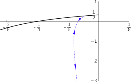
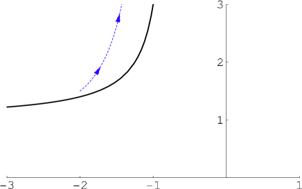
Figure 3: The time evolution for $\Lambda_{B}=0$ in the three regions for different initial conditions: $w_{0}=0,1/3,2/3$ for the region I, $w_{0}=-1$ for the region II and $w_{0}=3/2$ for region III. The thick lines correspond to the boundaries (58), (59) of the three regions and the stars to the initial conditions. The thick dot represents the fixed point of the evolution.

The time evolutions for regions II (see case II in Fig. 3) and III (see case III in Fig. 3) have on the other hand different characteristics. This is because there is no corresponding isotropic fixed points towards they could evolve.

In region II, the system evolves towards the boundary line, is reflected back and evolves asymptotically to $\rho_{m}\to 0^{-}$ at $w\to-\infty$. The anisotropy increases as the boundary line is approached and decreases $A\to\sqrt{2}$ at the asymptotics. Let us note also that although region II is connected to the fixed point $w=1/3$, we have seen no evolution towards this point. These cosmological evolutions give rise to a regular geometry at $r=0$ for initial conditions on the left of the lines of long dashing in the region II of Fig. 2c.

In region III, the system evolves towards the boundary line as $w\to\infty$ and $\alpha\rho_{m}/M_{Pl}^{2}\to-3/4$. The anisotropy decreases but tends to a constant value $A>\sqrt{2}$. These cosmological evolutions give always rise to a regular geometry at $r=0$.

From the above analysis we conclude that, the relaxation of the tuning relation between $w$ and $\rho_{m}$, has as a consequence the appearance of new branches of brane world evolution (regions II, III), while in region I the system tends quickly to the isotropic fixed point attractor. Furthermore, we observe that the anisotropy in all cases decreases much more quickly than in the four dimensional case with the same initial conditions but without the extra dimensional constraint.

6.2 Evolution of the System with $\Lambda_{B}\neq 0$

Studying the asymptotics for $w_{1}$ and $w_{2}$ from (58), (59) we find that for $\Lambda_{B}\neq 0$, there are three intervals of $\Lambda_{B}$ with different shape of the allowed regions in the $(\rho_{m},w)$ plane. The parameter space for these distinct cases is shown in Figs. 2a,b,d.

From the dynamical system (60), (61), (62) we see that there are two fixed points in general. The first one is the same with that of the isotropic evolution, i.e.,

$$(\rho_{m},H^{2}_{a},H^{2}_{b},w)=\left(\rho_{f},{\rho_{f}\over 3M_{Pl}^{2}},0,-1\right)~{},$$ (65)

with ${\alpha\rho_{f}\over M_{Pl}^{2}}=-{3\over 4}+{3\over 4}\sqrt{1+{4\over 3}{\alpha\Lambda_{B}\over M_{6}^{4}}}$ and it exists only for $\Lambda_{B}>0$. Linear perturbation around this point reveals again that it is an attractor.

The second fixed point that we find is

$$(\rho_{m},H^{2}_{a},H^{2}_{b},w)=\left(-\Lambda_{B}{M_{Pl}^{2}\over M_{6}^{4}},0,{\Lambda_{B}\over M_{6}^{4}},1\right)~{}.$$ (66)

and it exists only for $\Lambda_{B}>0$. Linear perturbation around this point reveals that it is a repeler.

Whenever the previous attractor fixed point exists, the system will be driven towards a final isotropic de Sitter state. The way in which this fixed point is approached from an arbitrary initial energy density, can tell us whether the line of isotropic tuning is an attractor or not. To analyze the features of the anisotropic evolutions, we will again proceed numerically.

For ${\alpha\Lambda_{B}\over M_{6}^{4}}>{3\over 4}$, the three allowed regions of the $(\rho_{m},w)$ plane are connected (see Fig. 2a). However, we can see numerically that any evolutions with initial conditions in one of the three regions, stays in that region. In other words, there can be no crossing of the ${\alpha\rho_{m}\over M_{Pl}^{2}}=-{3\over 4}$ or ${\alpha\rho_{m}\over M_{Pl}^{2}}=0$ lines. In region I the system evolves quickly towards the line of isotropic tuning and tracks it until the attractor fixed point of $w=-1$ is reached. We can see numerically that anisotropy falls to zero like $A\sim\exp\left[-{\cal O}(1)\sqrt{{\alpha\Lambda_{B}\over M_{6}^{4}}}~{}t\right]$ and thus the line of isotropic tuning is attracting very strongly the evolution of the system towards it. In region II, the system evolves towards $\rho_{m}\to 0^{-}$ and $w\to+\infty$. Its anisotropy decreases and in the asymptotics it tends to $A\to\sqrt{2}$. In region III the system evolves to $w\to+\infty$ and $\alpha\rho_{m}/M_{Pl}^{2}\to-3/4$. The anisotropy decreases, but tends to a constant value $A>\sqrt{2}$.

For $0<{\alpha\Lambda_{B}\over M_{6}^{4}}<{3\over 4}$, two of the allowed regions of the $(\rho_{m},w)$ plane are connected (see Fig. 2b). We can again verify numerically that any evolutions with initial conditions in one of these two regions, stays in that region, so that there is no crossing of the ${\alpha\rho_{m}\over M_{Pl}^{2}}=0$ line. In region I the system tracks the line of isotropic tuning and evolves towards the attractor fixed point of $w=-1$ while it isotropises ($A\to 0$). The anisotropy falls to zero again like $A\sim\exp\left[-{\cal O}(1)\sqrt{{\alpha\Lambda_{B}\over M_{6}^{4}}}~{}t\right]$ and thus, the line of isotropic tuning is an attractor. However, the strength of the attractor can be very weak in the cases when ${\alpha\Lambda_{B}\over M_{6}^{4}}\ll 1$. In region II, the system evolves towards $\rho_{m}\to 0^{-}$ and $w\to+\infty$. Its anisotropy decreases and in the asymptotics it tends to $A\to\sqrt{2}$. In region III the system again evolves to $w\to+\infty$ and $\alpha\rho_{m}/M_{Pl}^{2}\to-3/4$. The anisotropy decreases, but tends to a constant value $A>\sqrt{2}$.

For ${\alpha\Lambda_{B}\over M_{6}^{4}}<0$, all allowed regions of the $(\rho_{m},w)$ plane are disconnected (see Fig. 2d). In region I the system evolves towards $\rho_{m}\to 0^{+}$ and $w\to+\infty$. Its anisotropy increases and tends in the asymptotics to $A\to\sqrt{2}$. In region II, the system evolves towards $\rho_{m}\to 0^{-}$ and $w\to-\infty$ in the same way as in the $\Lambda_{B}=0$ case. Its anisotropy decreases and in the asymptotics it tends to $A\to\sqrt{2}$. In region III the system again evolves to $w\to+\infty$ and $\alpha\rho_{m}/M_{Pl}^{2}\to-3/4$. The anisotropy decreases, but tends to a constant value $A>\sqrt{2}$.

The evolutions in the three regions resemble the ones plotted in Fig. 3 for the $\Lambda_{B}=0$ case. In all three regions the cosmological evolutions give rise to a regular geometry at $r=0$ when the initial conditions are such that the system never crosses the lines of long dashing in Figs. 2a,b,d. For example, this happens for the evolutions in the region I for $\Lambda_{B}>0$ and $w_{s}^{-}<-1<w<w_{s}^{+}$.

From the above we conclude that, the relaxation of the tuning between $w$ and $\rho_{m}$, has as a consequence the appearance of new branches of brane world evolution (regions II, III), while in region I the system tends to the attractor fixed points, whenever they exist. For the cases when $\Lambda_{B}>0$ the lines of isotropic tuning are attractors, with strength depending on the value of $\Lambda_{B}$.

Furthermore, we observe that the anisotropy in all cases, apart the one of region I for $\Lambda_{B}<0$, decreases much more quickly than in the four dimensional case, with the same initial conditions, but without the extra dimensional constraint. In region I for $\Lambda_{B}<0$, the anisotropy increases and is larger than the one of the purely four dimensional case.

Figure 4: The evolution of the equation of state $w$ and the anisotropy $A$ for the case of $\alpha\Lambda_{B}/M_{6}^{4}=10^{-4}$ with initial condition $w_{0}=2/3$. Until the fixed point is approached ($w\sim-1$), we have significant anisotropy $A\sim{\mathcal{O}}(1)-{\mathcal{O}}(10^{-1})$.

Let us now examine again the interesting possibility of $0<\alpha\Lambda_{B}/M_{6}^{4}\ll 1$ with the transition between $w=1/3$ to $w=0$ and finally to $w=-1$. As it can be inferred from the previous discussion, the system tracks the line of isotropic tuning and evolves towards the attractor fixed point with $w=-1$ (see Fig. 4). However, due to the small value of $\alpha\Lambda_{B}/M_{6}^{4}$, the line of isotropic tuning is a very weak attractor. Most of the evolution is rather anisotropic with $A\sim{\mathcal{O}}(1)-{\mathcal{O}}(10^{-1})$ until the fixed point is approached, in which region it drops to zero.

This large anisotropy makes the cosmological evolution phenomenologically problematic. In order that the anisotropy is acceptably small, the initial conditions for the energy density and the equation of state should be fine tuned to lie very close to the line of isotropic tuning initially.

In conclusion, by analyzing the anisotropic dynamics of the system we have seen that the lines of isotropic tuning are attractors for $\Lambda_{B}>0$, with $\Lambda_{B}$-dependent attracting strength. The most phenomenologically accepted evolutions with $0<\alpha\Lambda_{B}/M_{6}^{4}\ll 1$ do not isotropise quickly enough and thus need a fine tuning in order to evolve with acceptable anisotropy.

7 Conclusions

In this work, we studied the cosmological dynamics of a conical codimension-2 brane-worlds. We considered a theory with a Gauss-Bonnet term in the six-dimensional bulk and an induced gravity term on the three-brane. For simplicity, we considered that the bulk matter consists only of a cosmological constant $\Lambda_{B}$ but the brane matter is general and isotropic. We then analyzed in detail the Einstein equations evaluated on the boundary.

We studied the system first for an isotropic metric ansatz. As was noted in [13], in the pure induced gravity dynamics there is a tuning between the matter allowed on the brane and in the bulk. This tuning, when the matter in the bulk is only a cosmological constant, gives a precise relation between the matter density on the brane and its equation of state. If a Gauss-Bonnet term is added in the bulk, the constraint equation giving the previous tuning is modified by the addition of a Riemann squared term. However, since for isotropic evolutions the Riemann tensor can be expressed in terms of the Ricci tensor and the scalar curvature, the conclusion about the presence of the tuning remains the same as in the induced gravity case.

We therefore considered the combination of the two effects for the isotropic metric ansatz and made the further simplifying assumption that the brane contains a tension contribution which gives a four-dimensional Einstein equation without a cosmological constant. The dynamics of the system of the four-dimensional equations plus the constraint equation of the extra dimensions, depend on the value of $\Lambda_{B}$. If $\Lambda_{B}>0$ the fixed point has $w=-1$ and corresponds to a de Sitter vacuum. If $\Lambda_{B}=0$, the system has a fixed point with equation of state $w=1/3$. Both of the previous fixed points are attractors. If $\Lambda_{B}<0$ the system has no fixed point and the evolutions exhibit a runaway behaviour to $w\to+\infty$.

The tight restriction on initial conditions on matter on the brane that the constraint equation imposes in the isotropic case, motivated us to look at the case where the initial ansatz is anisotropic. In this way, we could determine whether the above tuning corresponds to an attractor. For this purpose, we considered a particular kind of anisotropy. Since the Riemann tensor in this case cannot be expressed in terms of the Ricci tensor and the scalar curvature, the previous studied constraint becomes now a dynamical equation for the anisotropy of the brane-world volume. The matter on the brane and its equation of state, need not lie on the line of isotropic tuning, but can have values in vast regions of parametric space which was previously forbidden. There are always three distinct regions of parametric space, one of which has as a boundary the line of isotropic tuning.

The dynamics of the system of the four-dimensional equations plus the extra dimensional equation, depend again on the value of $\Lambda_{B}$. If the system starts its evolution in the region of parametric space which has as a boundary the line of isotropic tuning, it tracks the latter line and isotropises towards the attractor fixed point with $w=-1$ for $\Lambda_{B}>0$, or the one with $w=1/3$ for $\Lambda_{B}=0$. In the two other regions the system has a runaway behaviour $w\to\infty$ and does not isotropise. For $\Lambda_{B}<0$, the system has always a runaway behaviour. The important result of this analysis is that the line of isotropic tuning, coming from the constraints found in [13], is an attractor. However, for values of $\Lambda_{B}$ which give acceptable cosmological evolutions, a fine tuning is unavoidable because of the weak strength of the above-mentioned attractor.

The above conclusions rely on the specific assumptions that we have made in order to simplify the dynamics of the system and might be altered if we change them. Let us remind the reader once again what has been assumed in the above analysis which may affect our final conclusions. Firstly, we consider only conical branes and in order to study cosmology on them we consider certain corrections to the gravity action (induced curvature and Gauss-Bonnet term). Secondly, we assume that the bulk matter has only the form of a cosmological constant. Thirdly, in studying the cosmological dynamics we consider that the tension contribution of the brane matter cancels the one induced by the deficit angle. Finally, there is an implicit assumption in this work that the complicated bulk equations of motion, when integrated away from the brane, are well behaved (e.g., no singularities).

Understanding the dynamics of codimension-2 branes is interesting because of the improvement they may make to the cosmological constant problem. There have been several models of self tuning relying on the properties of codimension-2 branes, where the vacuum energy of the brane does not curve the brane world-volume without fine tuning. It would be interesting to see what the cosmology of these models would be by repeating the above analysis for a bulk content which is provided by these models.

References

- [1]
- [2] P. Binetruy, C. Deffayet and D. Langlois, Nucl. Phys. B 565 (2000) 269 [arXiv:hep-th/9905012], P. Binetruy, C. Deffayet, U. Ellwanger and D. Langlois, Phys. Lett. B 477 (2000) 285 [arXiv:hep-th/9910219], C. Csaki, M. Graesser, L. Randall and J. Terning, Phys. Rev. D 62 (2000) 045015 [arXiv:hep-ph/9911406], P. Kanti, I. I. Kogan, K. A. Olive and M. Pospelov, Phys. Rev. D 61 (2000) 106004 [arXiv:hep-ph/9912266], J. E. Kim, B. Kyae and H. M. Lee, Nucl. Phys. B 582 (2000) 296 [Erratum-ibid. B 591 (2000) 587] [arXiv:hep-th/0004005], R. Maartens, Phys. Rev. D 62 (2000) 084023 [arXiv:hep-th/0004166], P. Bowcock, C. Charmousis and R. Gregory, Class. Quant. Grav. 17, 4745 (2000) [arXiv:hep-th/0007177], C. Deffayet, Phys. Lett. B 502 (2001) 199 [arXiv:hep-th/0010186], C. Charmousis and J. F. Dufaux, Class. Quant. Grav. 19 (2002) 4671 [arXiv:hep-th/0202107], G. Kofinas, R. Maartens and E. Papantonopoulos, JHEP 0310 (2003) 066 [arXiv:hep-th/0307138].
- [3] R. Maartens, D. Wands, B. A. Bassett and I. Heard, Phys. Rev. D 62 (2000) 041301 [arXiv:hep-ph/9912464], J. E. Lidsey and N. J. Nunes, Phys. Rev. D 67, 103510 (2003) [arXiv:astro-ph/0303168], A. R. Liddle and A. J. Smith, Phys. Rev. D 68, 061301 (2003) [arXiv:astro-ph/0307017], E. Papantonopoulos and V. Zamarias, JCAP 0410, 001 (2004) [arXiv:gr-qc/0403090], G. Calcagni, Phys. Rev. D 69, 103508 (2004) [arXiv:hep-ph/0402126].
- [4] C. Deffayet, G. R. Dvali and G. Gabadadze, Phys. Rev. D 65 (2002) 044023 [arXiv:astro-ph/0105068], V. Sahni and Y. Shtanov, Int. J. Mod. Phys. D 11, 1515 (2000) [arXiv:gr-qc/0205111], V. Sahni and Y. Shtanov, JCAP 0311, 014 (2003) [arXiv:astro-ph/0202346].
- [5] M. Kolanovic, M. Porrati and J. W. Rombouts, Phys. Rev. D 68 (2003) 064018 [arXiv:hep-th/0304148], S. Kanno and J. Soda, JCAP 0407 (2004) 002 [arXiv:hep-th/0404207], J. Vinet and J. M. Cline, Phys. Rev. D 70 (2004) 083514 [arXiv:hep-th/0406141], I. Navarro and J. Santiago, JHEP 0502, 007 (2005) [arXiv:hep-th/0411250], J. Vinet and J. M. Cline, Phys. Rev. D 71, 064011 (2005) [arXiv:hep-th/0501098], G. Kofinas, arXiv:hep-th/0506035.
- [6] H. Collins and B. Holdom, Phys. Rev. D 62 (2000) 105009 [arXiv:hep-ph/0003173], G. R. Dvali, G. Gabadadze and M. Porrati, Phys. Lett. B 485 (2000) 208 [arXiv:hep-th/0005016], G. R. Dvali and G. Gabadadze, Phys. Rev. D 63 (2001) 065007 [arXiv:hep-th/0008054].
- [7] D. Lovelock, J. Math. Phys. 12 (1971) 498, C. Charmousis and R. Zegers, arXiv:hep-th/0502171, N. E. Mavromatos and E. Papantonopoulos, arXiv:hep-th/0503243.
- [8] E. Gravanis and S. Willison, arXiv:gr-qc/0401062, H. M. Lee and G. Tasinato, JCAP 0404 (2004) 009 [arXiv:hep-th/0401221], I. Navarro and J. Santiago, JHEP 0404 (2004) 062 [arXiv:hep-th/0402204].
- [9] J. W. Chen, M. A. Luty and E. Ponton, JHEP 0009 (2000) 012 [arXiv:hep-th/0003067].
- [10] S. M. Carroll and M. M. Guica, [arXiv:hep-th/0302067], I. Navarro, JCAP 0309 (2003) 004 [arXiv:hep-th/0302129], Y. Aghababaie, C. P. Burgess, S. L. Parameswaran and F. Quevedo, Nucl. Phys. B 680 (2004) 389 [arXiv:hep-th/0304256], I. Navarro, Class. Quant. Grav. 20 (2003) 3603 [arXiv:hep-th/0305014], G. W. Gibbons, R. Guven and C. N. Pope, Phys. Lett. B 595 (2004) 498 [arXiv:hep-th/0307238], H. P. Nilles, A. Papazoglou and G. Tasinato, Nucl. Phys. B 677 (2004) 405 [arXiv:hep-th/0309042], H. M. Lee, Phys. Lett. B 587 (2004) 117 [arXiv:hep-th/0309050], A. Kehagias, Phys. Lett. B 600 (2004) 133 [arXiv:hep-th/0406025], S. Randjbar-Daemi and V. Rubakov, JHEP 0410 (2004) 054 [arXiv:hep-th/0407176], H. M. Lee and A. Papazoglou, Nucl. Phys. B 705 (2005) 152 [arXiv:hep-th/0407208], V. P. Nair and S. Randjbar-Daemi, JHEP 0503, 049 (2005) [arXiv:hep-th/0408063], C. P. Burgess, F. Quevedo, G. Tasinato and I. Zavala, JHEP 0411 (2004) 069 [arXiv:hep-th/0408109], M. Redi, Phys. Rev. D 71, 044006 (2005) [arXiv:hep-th/0412189], G. Kofinas, Class. Quant. Grav. 22 (2005) L47 [arXiv:hep-th/0412299], C. P. Burgess, AIP Conf. Proc. 743, 417 (2005) [arXiv:hep-th/0411140], J. M. Schwindt and C. Wetterich, [arXiv:hep-th/0501049].
- [11] J. M. Cline, J. Descheneau, M. Giovannini and J. Vinet, JHEP 0306 (2003) 048 [arXiv:hep-th/0304147].
- [12] P. Bostock, R. Gregory, I. Navarro and J. Santiago, Phys. Rev. Lett. 92 (2004) 221601 [arXiv:hep-th/0311074].
- [13] E. Papantonopoulos and A. Papazoglou, JCAP 0507 (2005) 004 [arXiv:hep-th/0501112].
- [14] F. Leblond, R. C. Myers and D. J. Winters, JHEP 0107 (2001) 031 [arXiv:hep-th/0106140].
- [15] E. Papantonopoulos, [arXiv:gr-qc/0410032].