Brane Decay of a (4+n)-Dimensional Rotating
Black Hole: spin-0 particles

G. Duffy¹, C. Harris², P. Kanti³ and E. Winstanley⁴

¹ Department of Mathematical Physics, University College Dublin,
Belfield, Dublin 4, Ireland

² Cavendish Laboratory, University of Cambridge,
Madingley Road, Cambridge CB3 0HE, United Kingdom

³ Department of Mathematical Sciences, University of Durham,
Science Site, South Road, Durham DH1 3LE, United Kingdom

⁴ Department of Applied Mathematics, The University of Sheffield,
Hicks Building, Hounsfield Road, Sheffield S3 7RH, United Kingdom

Abstract

In this work, we study the ‘scalar channel’ of the emission of Hawking radiation from a $(4+n)$-dimensional, rotating black hole on the brane. We numerically solve both the radial and angular part of the equation of motion for the scalar field, and determine the exact values of the absorption probability and of the spheroidal harmonics, respectively. With these, we calculate the particle, energy and angular momentum emission rates, as well as the angular variation in the flux and power spectra – a distinctive feature of emission during the spin-down phase of the life of the produced black hole. Our analysis is free from any approximations, with our results being valid for arbitrarily large values of the energy of the emitted particle, angular momentum of the black hole and dimensionality of spacetime. We finally compute the total emissivities for the number of particles, energy and angular momentum and compare their relative behaviour for different values of the parameters of the theory.

1 Introduction

The formulation of the theory with Large Extra Dimensions [1] was driven by the motivation to address the hierarchy problem (for some early works, see [2]). While all Standard Model fields are restricted to live on a (3+1)-dimensional brane, gravity is allowed to propagate in the $(4+n)$-dimensional bulk; above the scale of decompactification of extra dimensions $M_{*}$, that can be as low as 1 TeV, gravitational interactions become strong and thus comparable to the Electroweak interactions. Moreover, above $M_{*}$, all effective theories cease to be valid, and a more fundamental theory, that describes all forces including gravity, must take over. In the context of such a theory, transplanckian collisions of particles become particularly important as their product cannot be ordinary particles any more but rather heavy objects. This opens up the exciting possibility of observing strong gravitational phenomena, linked to a Quantum Theory of Gravity, at a low energy scale, possibly at the TeV scale.

The creation of mini black holes as the result of such transplanckian particle collisions [3] has drawn considerable interest during the last few years. Such black holes may be created either at colliders [4] or in high energy cosmic-ray interactions [5] (for an extensive discussion of the phenomenological implications and a more complete list of references, see the reviews [6, 7, 8]). If the produced black holes have a mass considerably larger than the fundamental Planck mass $M_{*}$, quantum gravity effects can be safely ignored, and the black holes can be treated as classical objects. Their most important characteristic, as well as the most prominent signature of their creation, will be the emission of Hawking radiation in the form of elementary particles. This will take place both in the bulk and on the brane, with the latter ‘channel’ being the most important from the phenomenological point of view. After shedding all additional quantum numbers during a short balding phase, as dictated by the no-hair theorem of General Relativity, the produced black hole will settle down to a Kerr-like phase, the spin-down phase, during which the black hole will mainly lose its angular momentum through the emission of Hawking radiation and superradiance. After that, the Schwarzschild phase will commence with the black hole (now spherically symmetric) emitting Hawking radiation and gradually losing its actual mass.

The Schwarzschild phase of the life of a small higher-dimensional black hole formed in a flat background has been admittedly the most well studied in the literature. The task of determining the spectrum of Hawking radiation during this phase has been attacked both analytically [9, 10, 11] and numerically [12]. While the first set of works led to the derivation of useful, analytical formulae for the emission rate, the latter work provided exact, numerical results valid at all energy regimes. Both approaches reached the conclusion that the Hawking radiation spectrum strongly depends on the existence of additional spacelike dimensions in nature, with this dependence being reflected both in the number of particles and energy emitted by the black hole per unit time as well as in the actual type of particles emitted (scalars vs. fermions vs. gauge bosons). Further studies have also shed light on the dependence of Hawking radiation from a higher-dimensional black hole on higher-derivative gravitational (Gauss-Bonnet) terms [13], the mass of the emitted particles [14, 15], the charge of the black hole [16], and last but not least, the cosmological constant [17], with the latter leading to a distinct signature of its existence at the low-energy part of the radiation spectrum.

The progress in studying the emission of Hawking radiation during the spin-down phase of a small, higher-dimensional black hole has been much slower. This was due to the more complicated gravitational background but also to additional technical difficulties in solving the equation of motion for a particle propagating in such a background. Analytical formulae for the emission rate were derived [18, 19] but the results were partial, being valid only at the low-energy regime, for low angular momentum of the black hole, and for a specific dimensionality of spacetime. The first exact numerical results for the Hawking radiation emission rate in the form of scalar fields, during the spin-down phase, as well as for the amplification due to superradiance, were presented in [20]. These were valid for arbitrary values of the energy of the emitted particle and for arbitrary values of the angular momentum parameter of the black hole. That was the result of the determination of the exact value of the angular eigenvalue – being also involved in the radial part of the equation of motion of the particle – via numerical means instead of the use of an approximate analytical formula. The analysis in [20] demonstrated that the suppression of the energy emission rate at the low-energy regime as the angular momentum of the black hole increases, as was found in [19], is in fact overturned in the intermediate- and higher-energy regime where a strong enhancement appears instead. In the case of superradiance, these results confirmed the existence of the effect in the higher-dimensional case, and demonstrated the exact energy amplification: although strongly mode-dependent, this amplification can reach approximately a 10% magnitude . Shortly afterwards, another study appeared in the literature [23], focused on the study of the power (energy) spectrum, as well as its angular distribution in the 5-dimensional case, but once more the analysis relied on the assumption of low energy and low angular momentum. Two more studies focused on 5-dimensional rotating black holes appeared recently [24, 25], where the question of the emission in the bulk was also addressed.

At present, a comprehensive study of the emission of Hawking radiation from a higher-dimensional black hole in its spin-down phase, that could provide exact numerical results for arbitrary values of the angular momentum of the black hole, the energy of the emitted particle and the dimensionality of spacetime, is still missing from the literature. Apart from the power (energy) spectrum, whose study needs to be completed for arbitrary values of the aforementioned parameters, the question of the emission rate of particles (flux spectrum) and of the rate of loss of angular momentum of the rotating black hole also needs to be addressed. Moreover, the angular distribution of the emitted radiation – a distinctive signature of emission from a rotating higher-dimensional black hole – needs to be investigated, with the results again being free from any restrictive assumption about the values of the fundamental parameters of the theory. It is these tasks that we have undertaken to fulfil in this work. The strongly spin-dependent techniques needed to be applied for the calculation of the spectra for different types of particles, and the plethora of results that need to be derived in each case, have forced us to restrict our attention in this work to the case of scalar fields emitted by the black hole, and present the corresponding analysis and results for higher-spin fields in a subsequent work [26].

Before presenting the outline of our paper, a brief discussion of the assumptions made during our analysis should be added here. As mentioned earlier, it will be assumed that the black hole mass $M_{BH}$ is considerably larger than the fundamental scale of gravity $M_{*}$ in order to ensure that quantum effects are small and that the black hole geometry can be safely considered as a classical object. The same constraint guarantees the absence of any significant back reaction to the gravitational background due to the change in the black hole mass after the emission of a particle: the assumption that the temperature of the black hole, around which the emission spectrum is centered, is much smaller than the black hole mass translates again to $M_{BH}\gg M_{*}$. We are also going to assume that the horizon of the black hole $r_{h}$ is much smaller than the (common) size $L$ of the additional compact spacelike dimensions so that the black hole can be considered as embedded in a $(4+n)$-dimensional, non compact, empty spacetime. Finally, since the value of the brane self-energy can be naturally assumed to be of the order of the fundamental Planck scale $M_{*}$, and thus much smaller than the black hole mass, its effect on the gravitational background can be ignored.

We will start, in Section 2, by presenting the theoretical framework for our analysis including basic formulae for the gravitational background, the equation of motion for the propagation of a scalar field in it, and the Hawking radiation emission spectra. In section 3, a description of the numerical methods and techniques used for the determination of the exact value of the angular eigenvalue and of the angular and radial part of the wavefunction of the field will be given. After the angular eigenvalue is determined, the radial part of the equation of motion is numerically solved to determine the absorption probability (greybody factor) and thus the various spectra. In section 4, we present our results for the flux, power and angular momentum spectra (integrated over the azimuthal angle $\theta$) for arbitrary values of the energy of the particle, the angular momentum of the black hole, and the dimensionality of spacetime. All the spectra have a thermal profile in terms of the energy of the particle, as expected, and bear a strong dependence on the value of the angular momentum of the black hole and the number of extra dimensions. Next, we numerically solve the angular part of the equation of motion to find the exact values of the spheroidal harmonics, and we calculate the angular distribution of the flux and power spectrum; these results are also given in section 4, and, contrary to the emission of radiation during the Schwarzschild phase, are characterized by a strong angular variation. Finally, in the last part of section 4 we focus on the study of the various total emissivities (the total number of particles, energy and angular momentum emitted per unit time by the black hole in all frequencies) and compare their behaviour for different values of the dimensionality of spacetime and of the angular momentum of the black hole. We finish with a summary of our results and conclusions, in Section 5.

2 Theoretical Framework

The gravitational background around a $(4+n)$-dimensional, rotating, uncharged black hole was found by Myers & Perry [27], and in what follows we will use this line-element to describe the spin-down phase of a small, higher-dimensional black hole created by the collision of highly energetic particles. If we assume that the colliding particles are restricted to propagate on an infinitely-thin 3-brane, they will have a non-zero impact parameter only along our brane, and thus acquire only one non-zero angular momentum parameter about an axis in the brane. Such a higher-dimensional black hole will then be described by the following line-element [27]

$$ds^{2}=\biggl{(}1-\frac{\mu}{\Sigma\,r^{n-1}}\biggr{)}dt^{2}+\frac{2a\mu\sin^{2}\theta}{\Sigma\,r^{n-1}}\,dt\,d\varphi-\frac{\Sigma}{\Delta}\,dr^{2}-\Sigma\,d\theta^{2}$$

$$- \biggl{(}r^{2}+a^{2}+\frac{a^{2}\mu\sin^{2}\theta}{\Sigma\,r^{n-1}}\biggr{)}\sin^{2}\theta\,d\varphi^{2}-r^{2}\cos^{2}\theta\,d\Omega_{n},$$ (1)

where

$$\Delta=r^{2}+a^{2}-\frac{\mu}{r^{n-1}}\,,\qquad\Sigma=r^{2}+a^{2}\,\cos^{2}\theta\,,$$ (2)

and $d\Omega_{n}$ is the line-element on a unit $n$-sphere. The mass and angular momentum (transverse to the $r\varphi$-plane) of the black hole are then given by

$$M_{BH}=\frac{(n+2)A_{n+2}}{16\pi G}\,\mu\,,\qquad J=\frac{2}{n+2}\,M_{BH}\,a\,,$$ (3)

with $G$ being the $(4+n)$-dimensional Newton’s constant, and $A_{n+2}$ the area of a $(n+2)$-dimensional unit sphere given by

$$A_{n+2}=\frac{2\pi^{(n+3)/2}}{\Gamma[(n+3)/2]}\,.$$ (4)

In this work, we will focus on the emission of Hawking radiation [28], in the form of scalar fields, from this $(4+n)$-dimensional, rotating black hole . For phenomenological reasons, we will concentrate on the emission of these fields directly on our brane since any particle modes emitted in the bulk cannot be detected by an observer restricted to live on the brane. We will thus need to determine first the line-element on which the brane-localized modes propagate, and then to solve their equation of motion on the resulting background. The induced-on-the-brane line-element can be found by fixing the values of the additional angular coordinates that were introduced to describe the compact extra $n$ dimensions: by setting $\theta_{i}=\pi/2$, for $i=2,...,n+1$, we are led to the 4-dimensional background

$$\begin{split}ds^{2}=\left(1-\frac{\mu}{\Sigma\,r^{n-1}}\right)dt^{2}&+\frac{2a\mu\sin^{2}\theta}{\Sigma\,r^{n-1}}\,dt\,d\varphi-\frac{\Sigma}{\Delta}dr^{2}\\[8.53581pt] &-\Sigma\,d\theta^{2}-\left(r^{2}+a^{2}+\frac{a^{2}\mu\sin^{2}\theta}{\Sigma\,r^{n-1}}\right)\sin^{2}\theta\,d\varphi^{2}\,.\end{split}$$ (5)

The black hole horizon is given by solving the equation $\Delta(r)=0$, which, for $n\geq 1$, leads to a unique solution given by

$$r_{h}^{n+1}=\frac{\mu}{1+a_{*}^{2}}\,,$$ (6)

where we have defined $a_{*}=a/r_{h}$. In addition, while for $n=0$ and $n=1$, there is a maximum possible value of $a$, that guarantees the existence of a real solution to the equation $\Delta=0$ and thus of a horizon, for $n>1$ there is no fundamental upper bound on $a$ and a horizon $r_{h}$ always exists. An upper bound can nevertheless be imposed on the angular momentum parameter of the black hole by demanding the creation of the black hole itself from the collision of the two particles. The maximum value of the impact parameter between the two particles that can lead to the creation of a black hole was found to be [8]

$$b_{\text{max}}=2\,\biggl{[}1+\biggl{(}\frac{n+2}{2}\biggr{)}^{2}\biggr{]}^{-\frac{1}{(n+1)}}\mu^{\frac{1}{(n+1)}}\,,$$ (7)

an analytic expression that is in very good agreement with the numerical results produced in [3]c. Then, by writing $J=bM_{BH}/2$, for the angular momentum of the black hole, and using Eq. (6) and the second of Eq. (3), we obtain

$$a^{\text{max}}_{*}=\frac{n+2}{2}\,.$$ (8)

The equation of motion for a particle with spin 0, 1/2 or 1, propagating in the induced-on-the-brane gravitational background (5) of a higher-dimensional, rotating black hole was derived in [6, 19]. For scalar fields, the field factorization

$$\phi(t,r,\theta,\varphi)=e^{-i\omega t}\,e^{im\varphi}\,R(r)\,T^{m}_{\ell}(\theta,a\omega)\,,$$ (9)

where $T^{m}_{\ell}(\theta,a\omega)$ are the so-called spheroidal harmonics [32], leads to the following set of decoupled radial and angular equations

$$\frac{d}{dr}\biggl{(}\Delta\,\frac{dR_{\omega\ell m}}{dr}\biggr{)}+\left(\frac{K^{2}}{\Delta}-\Lambda^{m}_{\ell}\right)R_{\omega\ell m}=0\,,$$ (10)

$$\frac{1}{\sin\theta}\frac{d}{d\theta}\left(\sin\theta\,\frac{dT^{m}_{\ell}(\theta,a\omega)}{d\theta}\right)+\biggl{(}-\frac{m^{2}}{\sin^{2}\theta}+a^{2}\omega^{2}\cos^{2}\theta+E^{m}_{\ell}\biggr{)}T^{m}_{\ell}(\theta,a\omega)=0\,,$$ (11)

respectively. In the above, we have defined

$$K=(r^{2}+a^{2})\,\omega-am\,,\qquad\Lambda^{m}_{\ell}=E^{m}_{\ell}+a^{2}\omega^{2}-2am\omega\,.$$ (12)

The angular eigenvalue $E^{m}_{\ell}$ provides a link between the angular and radial equation, and various methods for finding its exact value will be discussed in the next section. Both equations (10)-(11) will be solved numerically to determine the radial and angular parts of the scalar field. The radial equation (10) can be solved analytically in the asymptotic regimes of near horizon and infinity. By using the new radial, ‘tortoise’, coordinate

$$\frac{dr^{*}}{dr}=\frac{r^{2}+a^{2}}{\Delta(r)}\,,$$ (13)

we find the following asymptotic solution near the horizon of the black hole

$$R_{h}(r^{*})=A_{1}\,e^{ikr^{*}}+A_{2}\,e^{-ikr^{*}}\,,$$ (14)

where $A_{1,2}$ are integration constants, and $k$ is defined as

$$k=\omega-\frac{ma}{r_{h}^{2}+a^{2}}\,.$$ (15)

A boundary condition must be applied in the near-horizon regime to ensure that the solution contains only incoming modes; this is satisfied if we set $A_{1}=0$. On the other hand, for fixed $a_{*}$ and large $r$, the asymptotic solution at infinity takes the form

$$R_{\infty}(r)=B_{1}\,\frac{e^{i\omega r}}{r}+B_{2}\,\frac{e^{-i\omega r}}{r}\,,$$ (16)

where $B_{1,2}$ are again integration constants. The asymptotic solutions (14) and (16) will serve as boundary conditions for our numerical analysis.

The Hawking temperature of the $(4+n)$-dimensional, rotating black hole is found to be

$$T_{\text{H}}=\frac{(n+1)+(n-1)a_{*}^{2}}{4\pi(1+a_{*}^{2})r_{h}}\,,$$ (17)

and leads to the emission of thermal Hawking radiation both in the bulk and on the brane. As mentioned earlier, here we will study the scalar field ‘channel’ emitted on the brane. Since we are interested in studying an evaporating black hole, the relevant quantum state is the “past” Unruh vacuum $|U^{-}\rangle$ [33, 34, 35]. This state is defined in terms of the standard “in” and “up” modes, corresponding to unit initial particle flux at past null infinity and the past horizon, respectively [33, 34, 35]. At infinity, far from the black hole, the outward fluxes of energy $E$ and angular momentum $J$ can be expressed in terms of the components $T^{rt}$ and $T^{r}_{\varphi}$ of the renormalized stress-energy tensor for a quantum scalar field in the state $|U^{-}\rangle$ [34]:

$$\frac{dE}{dt} = \int_{S_{\infty}}\langle U^{-}|T^{rt}|U^{-}\rangle_{\rm{ren}}\,r^{2}\sin\theta\,d\theta\,d\varphi\,,$$

$$\frac{dJ}{dt} = \int_{S_{\infty}}\langle U^{-}|T^{r}_{\varphi}|U^{-}\rangle_{\rm{ren}}\,r^{2}\sin\theta\,d\theta\,d\varphi\,,$$ (18)

where the integral is taken over the sphere at infinity. These two components do not need renormalization for a quantum scalar field on the metric (5) [34], thus simplifying the computation. Our boundary conditions, (14) and (16), correspond to the “in” modes [33, 35], and in terms of these the relevant quantities can be written as

$$\langle U^{-}|T^{rt}|U^{-}\rangle_{\rm{ren}} = \frac{1}{4\pi^{2}r^{2}}\sum_{\ell,m}\int_{\omega=0}^{\infty}\frac{\omega\,d\omega}{\exp\left[k/T_{\text{H}}\right]-1}|{\cal A}_{\ell,m}|^{2}\,|T^{m}_{\ell}(\theta,a\omega)|^{2}\,,$$ (19)

$$\langle U^{-}|T^{r}_{\varphi}|U^{-}\rangle_{\rm{ren}} = \frac{1}{4\pi^{2}r^{2}}\sum_{\ell,m}\int_{\omega=0}^{\infty}\frac{m\,d\omega}{\exp\left[k/T_{\text{H}}\right]-1}|{\cal A}_{\ell,m}|^{2}\,|T^{m}_{\ell}(\theta,a\omega)|^{2}\,.$$ (20)

In the above expressions, $|{\cal A}_{\ell,m}|^{2}$ is the absorption (or transmission) probability for a scalar particle propagating in the brane background (5), and $k$ is given by (15). Multiplying these expressions by $r^{2}\sin\theta$ and integrating over the sphere at infinity gives the total outgoing fluxes of energy and angular momentum:

$$\frac{dE}{dt} = \frac{1}{2\pi}\sum_{\ell,m}\int_{\omega=0}^{\infty}\frac{\omega\,d\omega}{\exp\left[k/T_{\text{H}}\right]-1}|{\cal A}_{\ell,m}|^{2}\,,$$ (21)

$$\frac{dJ}{dt} = \frac{1}{2\pi}\sum_{\ell,m}\int_{\omega=0}^{\infty}\frac{m\,d\omega}{\exp\left[k/T_{\text{H}}\right]-1}|{\cal A}_{\ell,m}|^{2}\,,$$ (22)

where we have used the fact that the spheroidal harmonics $T^{m}_{\ell}(\theta,a\omega)$ are normalized according to

$$\int_{\theta=0}^{\pi}d\theta\,\sin\theta\,|T^{m}_{\ell}(\theta,a\omega)|^{2}=1.$$ (23)

The absorption probability $|{\cal A}_{\ell,m}|^{2}$ has an explicit dependence not only on the angular momentum numbers $(\ell,m)$, as denoted, but also on the energy $\omega$ of the emitted particle and the number of extra dimensions $n$. Therefore, its presence in the expressions of the emission rates modifies significantly the blackbody profile of the spectrum, especially in the low- and intermediate-energy regime. Its exact form will be found by solving numerically the radial equation (10) and determining the amplitudes of the incoming and outgoing modes at infinity, according to the asymptotic solution (16). Then, the absorption probability may be written as

$$|{\cal A}_{\ell,m}|^{2}=1-|{\cal R}_{\ell,m}|^{2}=1-\biggl{|}\frac{B_{1}}{B_{2}}\biggr{|}^{2}\,.$$ (24)

The first part of this work will focus on the computation of the differential emission rates of particles (flux spectrum), energy (power spectrum) and angular momentum, integrated over all angles $\theta$. These are given by

$$\frac{d^{2}N}{dtd\omega} = \frac{1}{2\pi}\sum_{\ell,m}\frac{1}{\exp\left[k/T_{\text{H}}\right]-1}|{\cal A}_{\ell,m}|^{2}\,,$$ (25)

$$\frac{d^{2}E}{dtd\omega} = \frac{1}{2\pi}\sum_{\ell,m}\frac{\omega}{\exp\left[k/T_{\text{H}}\right]-1}|{\cal A}_{\ell,m}|^{2}\,,$$ (26)

$$\frac{d^{2}J}{dtd\omega} = \frac{1}{2\pi}\sum_{\ell,m}\frac{m}{\exp\left[k/T_{\text{H}}\right]-1}|{\cal A}_{\ell,m}|^{2}\,.$$ (27)

By using the exact solutions of the angular equation (11), we will then study the angular distribution of the differential fluxes of particles and energy due to the axial symmetry of the gravitational background – a feature that will be a distinct signature of emission during the spin-down phase:

$$\frac{d^{3}N}{d(\cos\theta)dtd\omega}=\frac{1}{2\pi}\sum_{\ell,m}\frac{1}{\exp\left[k/T_{\text{H}}\right]-1}|{\cal A}_{\ell,m}|^{2}|T^{m}_{\ell}(\theta,a\omega)|^{2}\,,$$ (28)

$$\frac{d^{3}E}{d(\cos\theta)dtd\omega}=\frac{1}{2\pi}\sum_{\ell,m}\frac{\omega}{\exp\left[k/T_{\text{H}}\right]-1}|{\cal A}_{\ell,m}|^{2}|T^{m}_{\ell}(\theta,a\omega)|^{2}\,.$$ (29)

In both cases, the various spectra will be given as a function of the energy of the emitted mode $\omega$, but their dependence on the angular momentum parameter of the black hole and the dimensionality of spacetime will be also studied in detail.

3 Numerical Analysis

For the purpose of the analysis presented in this work, we will need to solve both the angular (11) and the radial (10) part of the scalar equation. The angular equation will be studied first as the eigenvalue $E^{m}_{\ell}$ is required before we can integrate the radial equation. The spheroidal harmonics, which are the solutions of Eq. (11), have been extensively studied in the literature [32], therefore, here we will only briefly outline our method and some of their key properties.

Before describing the numerical analysis performed in this work though, we would like to note that if one is interested in solving the radial equation only and studying the spectrum integrated over the angle $\theta$, then it is sufficient to find only the eigenvalues $E^{m}_{\ell}$, while the eigenfunctions $T^{m}_{\ell}(\theta,a\omega)$ are not required. The eigenvalues $E^{m}_{\ell}$ are functions of $a\omega$, and an analytic form exists only in the limit of small $a\omega$. To derive results for the emission of Hawking radiation valid for arbitrarily large energy of the emitted particle and angular momentum of the black hole, one needs to find numerically the exact value of $E^{m}_{\ell}$. This can be done, for instance, by using the so-called continuation method [36]. The continuation method is a generalization of perturbation theory which is applicable when the changes in the initial Hamiltonian (for which the eigenvalues are known) are not necessarily small. It involves writing the $T^{m}_{\ell}(\theta,a\omega)$ functions in the basis of the $\theta$-parts of the spherical harmonics, $S_{\ell}^{m}(\theta)$, which in conjunction with the angular equation and techniques from the perturbation theory leads to a differential equation for the eigenvalue $E^{m}_{\ell}$. This is, then, solved numerically, by using appropriate initial conditions, to derive the eigenvalue for any $\ell$ and $m$ and for any value of $a\omega$. This method was outlined in [8] and used in [20] for the derivation of the exact power spectrum for the emission of Hawking radiation, in the form of scalar fields, from a 5-dimensional black hole on the brane.

As mentioned above, in this work we also compute the exact angular distributions of the fluxes of particles and energy, therefore we require the values of the spheroidal harmonics $T^{m}_{\ell}(\theta,a\omega)$ themselves. For this, we follow a modified version of the method presented in section 17.4 of [37]. Given the symmetry in the angular equation (11) under the replacement of $m$ by $-m$, it is sufficient to consider only those solutions for which $m\geq 0$. It is also convenient to change the independent variable to $\eta=\cos\theta$ and define a new dependent variable $y_{\ell m\omega}$ by

$$y_{\ell m\omega}=\left(1-\eta^{2}\right)^{-\frac{m}{2}}T^{m}_{\ell}(\theta,a\omega),$$ (30)

in terms of which the angular equation (11) becomes

$$\left(1-\eta^{2}\right)\frac{d^{2}y_{\ell m\omega}}{d\eta^{2}}-2\left(m+1\right)\eta\frac{dy_{\ell m\omega}}{d\eta}+\left(E^{m}_{\ell}-m\left(m+1\right)+a^{2}\omega^{2}\eta^{2}\right)y_{\ell m\omega}=0\,.$$ (31)

The above equation must be solved on the interval $[-1,1]$, with the boundary conditions that $y_{\ell m\omega}$ is regular and non-zero at both end-points. We used a shooting method [37] to solve this boundary value problem. For spin 0 particles, the number of zeros of $y_{\ell m\omega}$ in the interval $[-1,1]$ is given by $\ell-m$, and the spheroidal harmonics are either odd or even functions of $\eta$. This symmetry can be used to integrate Eq. (31) over the half-interval $[-1,0]$, using appropriate boundary conditions at $\eta=0$. However, we have chosen not to take this path, but instead to integrate over the full interval $[-1,1]$ as this method will more readily generalize to higher spins [26], when the spin-weighted spheroidal harmonics do not have this symmetry property.

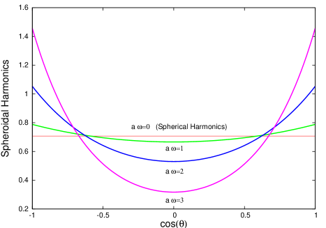
Figure 1: Spheroidal harmonics for a scalar field with $\ell=m=0$, and for $a\omega=(0,1,2,3)$.

The end-points, $\eta=\pm 1$, are regular singular points of Eq. (31). By using the Frobenius method, we find two linearly independent solutions near these end-points, one of which is regular and the other irregular. We begin the numerical integration at $\eta=-1+\delta\eta$, with $\delta\eta=10^{-7}$, using the Frobenius series expansion to impose our initial condition for a regular function $y$. We then integrate out to $\eta=1$, and demand that the solution be also regular at $\eta=1$. For a general initial value of $E^{m}_{\ell}$, the numerical solution, close to $\eta=1$, will be a linear combination of the regular solution we are seeking and the irregular solution. We define a function $F$, which depends on $E^{m}_{\ell}$, as follows:

$$F(E^{m}_{\ell})=\left.\frac{1}{y_{\rm{reg}}}\frac{dy_{\rm{reg}}}{d\eta}\right|_{\eta=1}-\left.\frac{1}{y}\frac{dy}{d\eta}\right|_{\eta=1}\,,$$ (32)

where $y$ is the numerical solution we have found by integration, and $y_{\rm{reg}}$ is the solution regular at $\eta=1$. The idea is therefore to find the value of $E^{m}_{\ell}$ such that $F(E^{m}_{\ell})=0$. Due to the irregular solution, the integration cannot be extended all the way to $\eta=1$, but instead we impose the boundary condition at $\eta=1-\delta\eta$, again using a Frobenius series expansion for the regular solution $y_{\rm{reg}}$.

The above method can give us the values of both the angular eigenvalues $E^{m}_{\ell}$ and the spheroidal harmonics $T^{m}_{\ell}(\theta,a\omega)$. In the case of the eigenvalues, we have used both the continuation and the shooting method, and we have found an excellent agreement between the values obtained. For the spheroidal eigenfunctions, the results found by using the shooting method  were finally normalized according to Eq. (23). In Fig. 1, as an illustrative example, we depict the derived spheroidal harmonics for the scalar mode with $\ell=m=0$, and for the values $a\omega=0,1,2$ and 3 – we remind the reader that, for $a\omega=0$, the spheroidal harmonics reduce to the spherical ones. In previous works [19, 23], the spherical harmonics were used as an approximation to the exact spheroidal ones. From Fig. 1, we can clearly see that, as long as $a\omega\ll 1$, this is indeed a valid approximation. However, as $a\omega$ increases, this approximation becomes increasingly poor. In addition, the difference between the spheroidal harmonics and the spherical ones is strongly mode-dependent, being more significant for the low ($\ell,m$) modes and less so for the high ($\ell,m$) modes. For an accurate analysis therefore, leading to the exact angular distribution of particle and energy fluxes, valid at all energy and angular momentum regimes, the use of the exact spheroidal harmonics is imperative.

Having derived the values of the angular eigenvalues $E_{\ell}^{m}$, the integration of the radial differential equation (10) can now proceed. We start the integration at the horizon of the black hole and integrate outwards towards infinity. Comparing our numerical results for the radial solution with the asymptotic solution at infinity (16), we determine the integration constants $B_{1}$ and $B_{2}$. The absorption probability for scalar fields can then be derived from the relation (24). The use of the exact value of the angular eigenvalue $E_{\ell}^{m}$, instead of an approximate analytical formula, guarantees the validity of the solution of the radial equation, too, for arbitrary energy of the emitted particle and angular momentum of the black hole.

4 Numerical Results

In this section, we present exact numerical results for the flux, power and angular momentum spectra for the emission of scalar particles on the brane from a higher-dimensional, rotating black hole. The dependence of the various spectra on the two fundamental parameters – the dimensionality of spacetime $n$ and the angular momentum parameter $a_{*}$ – will be studied in detail, and in the case of the first two types of spectra (flux and power), the angular distribution of the emitted particles and energy will also be examined. We will finally study the corresponding total emissivities of the black hole on the brane. These follow by integrating the various emission spectra over the whole frequency regime, and can provide information on the dependence of the total number of particles, energy and angular momentum, emitted by the black hole per unit time, on $n$ and $a_{*}$, as well as on their relative behaviour as the values of $n$ and $a_{*}$ vary.

4.1 Flux emission spectra

We start by presenting our numerical results for the number of scalar particles emitted by the black hole on the brane per unit time and unit frequency. Figures 2(a,b) depict the flux emission rate, Eq. (25), as a function of the frequency of the emitted particle in dimensionless units, $\omega r_{h}$, for various values of the angular momentum parameter $a_{*}$ of the black hole. The behaviour of the flux depends strongly also on the dimensionality of spacetime, and, for that reason, Figs. 2(a) and (b) present results for two indicative cases, $n=1$ and $n=4$, respectively.

\psfrag{x}[0.8]{$\omega\,r_{\text{h}}$}\psfrag{y}[0.8]{${r_{\text{h}}^{2}\,d^{2}N/dt\,d\omega}$}\includegraphics[height=159.3356pt,clip]{fluxs0n1.eps} \psfrag{x}[0.8]{$\omega\,r_{\text{h}}$}\psfrag{y}[0.8]{$r_{\text{h}}^{2}\,d^{2}N/dt\,d\omega$}\includegraphics[height=159.3356pt,clip]{fluxs0n4.eps}

Figure 2: Flux emission spectra for scalar particles on the brane from a rotating black hole, for (a) $n=1$, and (b) $n=4$, and various values of $a_{*}$.             

In the case of a 5-dimensional black hole, the particle flux, shown in Fig. 2(a), is characterized, for small values of $a_{*}$, by a strong peak at low values of $\omega r_{h}$; this clearly favours the emission of low-energy quanta. As the angular momentum parameter increases, however, this peaked Gaussian curve gives its place to a broad one, where high-energy particles become almost as equally likely to be emitted as the low- and intermediate-energy ones. This feature will be of prime importance in the determination of the power spectrum, to be studied in the next subsection. For higher values of $a_{*}$, oscillations become a common feature of the spectrum; these are due to the higher partial waves gradually coming into dominance as the energy increases. In Fig. 2(b), we depict the flux spectrum of an 8-dimensional rotating black hole. The spectrum shares common characteristics with the one obtained in the 5-dimensional case, with the curve becoming broader and the tail dying away much more slowly, as $a_{*}$ increases. However, there is now a clear enhancement in the number of particles emitted by the black hole per unit time over the whole energy regime, as $a_{*}$ increases, and the oscillations, although still present, are less apparent here.

Comparing the vertical axes of Figs. 2(a) and (b), one easily observes the almost one order-of-magnitude enhancement in the flux of particles, as we go from the $n=1$ to the $n=4$ case. This enhancement was a characteristic feature of the flux spectrum in the case of a non-rotating black hole [12], and – as we see in Fig. 3 – it characterizes also the spectrum of a rotating black hole. Figure 3 depicts the particle emission rate for a rotating black hole with a fixed angular momentum parameter, $a_{*}=1$, living in spacetimes with different dimensionalities. The particle flux broadly increases, and peaks for higher values of $\omega r_{h}$, as $n$ increases, clearly leading to a higher total number of particles emitted per unit time, as we will also see in subsection 3.4.

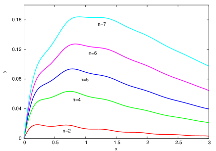
Figure 3: Flux emission spectra for scalar particles on the brane from a rotating black hole, with $a_{*}=1$, for various values of $n$.             

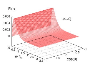
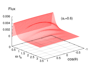
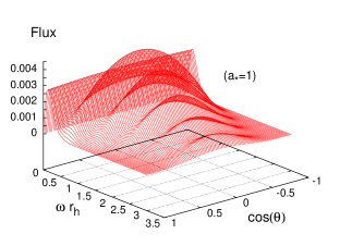
Figure 4: Angular distribution of the flux spectra for scalar emission on the brane from a rotating black hole, for $n=1$ and $a_{*}=(0,0.6,1)$.

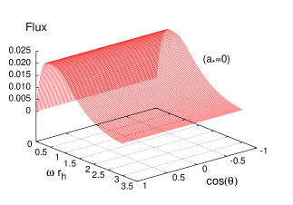
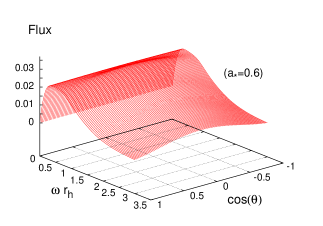
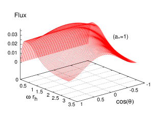
Figure 5: Angular distribution of the flux spectra for scalar emission on the brane from a rotating black hole, for $n=4$ and $a_{*}=(0,0.6,1)$.

Also of great importance is the angular distribution of the emitted particles. Whereas, in the case of a non-rotating black hole, we expect a uniform distribution of particles, in the case of a rotating black hole, we anticipate a distinctly different angular distribution pattern. An angular variation in the flux and power spectra would be a clear, characteristic signature for emission during the spin-down phase in the life of a black hole. Figures 4 and 5 depict the flux emission spectra on the brane from a rotating black hole with $n=1$ and $n=4$, respectively, and for $a_{*}=(0,0.6,1)$, as a function of the energy of the emitted particle and the value of $\cos\theta$ of the azimuthal angle. As expected, for vanishing $a_{*}$, the spectrum shows no angular variation, independently of the value of $n$. As the angular momentum parameter increases, the emitted modes are starting to concentrate on a region around the equator ($\theta=\pi/2$), however, their angular distribution depends, at the same time, also on their energy: even for non-vanishing $a_{*}$, at low energies the spectrum is dominated by a spherically-symmetric distribution, and shows no dependence on the angle $\theta$; only when the energy exceeds a certain value does the non-spherically-symmetric nature of the emission become significant. In general, for fixed $a_{*}$, as $n$ increases, the non-spherically-symmetric behaviour becomes dominant sooner, i.e. at lower energies, and there is an increasing contribution from angles away from the equator .

\psfrag{x}[0.8]{$\omega\,r_{\text{h}}$}\psfrag{y}[0.8]{$r_{\text{h}}\,d^{2}E/dt\,d\omega$}\includegraphics[height=159.3356pt,clip]{powers0n1.eps} \psfrag{x}[0.8]{$\omega\,r_{\text{h}}$}\psfrag{y}[0.8]{$r_{\text{h}}\,d^{2}E/dt\,d\omega$}\includegraphics[height=159.3356pt,clip]{powers0n4.eps}

Figure 6: Power emission spectra for scalar particles on the brane from a rotating black hole, for (a) $n=1$, and (b) $n=4$, and various values of $a_{*}$.             

4.2 Power emission spectra

We now move to the power spectrum that describes the energy emitted by the black hole on the brane in the form of scalar particles per unit time and unit frequency. As in the previous subsection, in Figs. 6(a,b), we display the energy emission spectra, for $n=1$ and $n=4$ respectively, as a function of the frequency of the emitted particle $\omega r_{h}$ and for various values of the angular momentum parameter $a_{*}$ of the black hole.

Since the energy emission rate follows by multiplying the particle emission rate by the frequency of the emitted particle, the numerical results shown in Figs. 6(a,b) can be easily justified by using the ones for the flux spectrum derived in the previous subsection. In the case of a 5-dimensional black hole, we found that, for small values of $a_{*}$, the black hole prefers to emit low-energy quanta, while, for higher values of $a_{*}$, the emission of low-energy particles is suppressed while that of intermediate- and high-energy particles becomes equally likely. Therefore, as the angular momentum parameter increases, we expect the energy emitted by the black hole per unit time to be suppressed in the low-energy regime, and to significantly increase in the high-energy regime – this is exactly the behaviour depicted in Fig. 6(a).

In the case of an 8-dimensional black hole, however, the flux spectrum [see Fig. 2(b)] shows no suppression even at the low-energy regime. As a result, the energy emission rate is uniformly enhanced, as $a_{*}$ increases, over the whole frequency regime. This behaviour, shown in Fig. 6(b), seems to be in disagreement with the one derived in Ref. [23], where the suppression at the low-energy regime in the power spectrum persists for all values – low or high – of the dimensionality of spacetime.

\psfrag{x}[0.8]{$\omega\,r_{\text{h}}$}\psfrag{y}[0.8]{$r_{\text{h}}\,d^{2}E/dt\,d\omega$}\includegraphics[height=159.3356pt,clip]{powers0a1.eps}

Figure 7: Power emission spectra for scalar particles on the brane from a rotating black hole, with $a_{*}=1$, for various values of $n$.             

Other features characterizing the flux spectra are also transferred almost intact to the power spectra. The oscillations make again their appearance, as the angular momentum increases, being quite prominent in the $n=1$ case and smoothed out for $n=4$. In both cases, the emission curves peak at higher values of $\omega r_{h}$ for larger values of $a_{*}$, signifying a clear enhancement of the total emission rate, as we will see in detail in Section 3.4. By comparing again the vertical axes of Figs. 6(a) and (b), an enhancement of more than one order-of-magnitude in the energy emission rate of the black hole is easily observed, as we go from $n=1$ to $n=4$. The enhancement in the power spectrum, as the dimensionality of spacetime increases, is clearly associated with the one found for the flux spectrum in the previous subsection, and is shown in detail in Fig. 7, for fixed $a_{*}$ and various values of $n$. A similar, strong enhancement in the power spectrum was also found in the case of a non-rotating black hole in [12], and independently confirmed by other subsequent works [15, 16, 17]. In the case of higher-dimensional, rotating black holes, the only other available results in the literature are the ones presented in [23]; however, the figures in that paper show only an infinitesimal enhancement of the power spectrum as $n$ increases, and curiously enough the enhancement is also missing from the results in [23] for the non-rotating, limiting case with $a_{*}=0$.

In Figs. 8 and 9, we depict the angular distribution of the power emission spectra from a rotating black hole on the brane for $n=1$ and $n=4$, respectively, and for $a_{*}=(0,0.6,1)$. Again, for vanishing $a_{*}$, the spectrum shows no angular variation, but, as the angular momentum parameter increases, the emitted modes are starting to concentrate on the region around the equator. At low-energies, the spectrum is again dominated by spherically symmetric behaviour, and thus remains independent of the angle $\theta$, but gradually the non-spherically-symmetric emission becomes important and an angular variation appears in the spectrum. As $a_{*}$ increases, we can clearly observe the enhancement in the energy emission rate as well as the shift of the peak of the curve towards higher values of $\omega r_{h}$. Similar behaviour, although on a much bigger scale, can be seen as we go from the $n=1$ to the $n=4$ case.

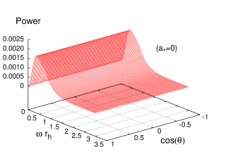
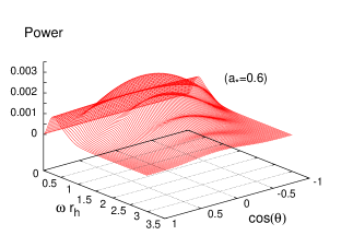
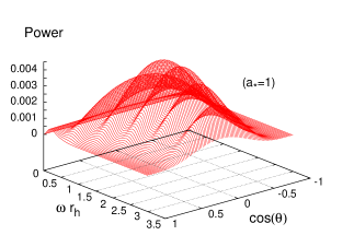
Figure 8: Angular distribution of the power spectra for scalar emission from rotating black holes, for $n=1$ and $a_{*}=(0,0.6,1)$.

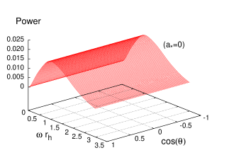
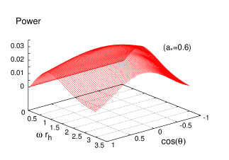
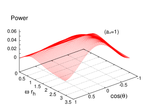
Figure 9: Angular distribution of the power spectra for scalar emission from rotating black holes, for $n=4$ and $a_{*}=(0,0.6,1)$.

The angular distribution of the power spectrum of a 5-dimensional black hole ($n=1$) was also studied in Ref. [23]. As mentioned before, these results were only approximate, in the sense that the spherical harmonics were used instead of the exact spheroidal ones (which is valid only for $a\omega\ll 1$). It would therefore be useful to compare those results with the ones derived here, and thus check the range of validity of the approximations made in Ref. [23]. By comparing our Figs. 8(a,b,c) (up to $\omega r_{h}=1$) with Figs. 8(a,b,c) in [23], we may see that an agreement arises in general terms: as $a_{*}$ increases, the emitted modes start to concentrate near the equator, oscillations appear, and the peak of the emission curve moves toward the right. Some differences though do appear, too: (i) in our case, the spherically symmetric emission becomes sub-dominant much faster, and the low-energy peak is rapidly suppressed, in contradiction with the behaviour depicted in Fig. 8 of Ref. [23]; (ii) the height of the peaks appearing at higher energies are also different, ours being in general lower compared to the ones in [23] - this could be explained by the fact that these peaks appear at energy values that are well beyond the range of the validity of the approximation $a\omega\ll 1$ made in Ref. [23]; (iii) finally, differences appear also in the $a_{*}=0$ case, with the emission curve dying out much faster in [23] than in our case.

\psfrag{x}[0.8]{$\omega\,r_{\text{h}}$}\psfrag{y}[0.8]{$r_{\text{h}}\,d^{2}J/dt\,d\omega$}\includegraphics[height=142.26378pt,clip]{angmoms0n1.eps}      \psfrag{x}[0.8]{$\omega\,r_{\text{h}}$}\psfrag{y}[0.8]{$r_{\text{h}}\,d^{2}J/dt\,d\omega$}\includegraphics[height=142.26378pt,clip]{angmoms0n4.eps}

Figure 10: Angular momentum spectra for scalar particles from a rotating black hole, for (a) $n=1$, and (b) $n=4$, and various values of $a_{*}$.             

\psfrag{x}[0.8]{$\omega\,r_{\text{h}}$}\psfrag{y}[0.8]{$r_{\text{h}}^{2}\,d^{2}J/dt\,d\omega$}\includegraphics[height=156.49014pt,clip]{angmoms0a1.eps}

Figure 11: Angular momentum spectra for scalar emission from a rotating black hole, for $a_{*}=1$ and various values of $n$.             

4.3 Angular momentum spectra

We now turn to the rate of loss of the angular momentum of the higher-dimensional, rotating black hole through the emission of scalar fields on the brane. In Figs. 10(a,b), this rate is shown, again, for the indicative cases of $n=1$ and $n=4$, respectively, and for various values of the angular momentum parameter $a_{*}$. As is clear from both figures, the emission of angular momentum is clearly enhanced at all frequencies, as $a_{*}$ increases, and for all values of $n$. For low values of $n$, oscillations are again present but, as in the case of flux and power emission, there is an ‘envelope’ of Gaussian shape whose height increases and which peaks at higher values of $\omega r_{h}$, as $a_{*}$ increases. For higher values of $n$, the oscillations are smoothed out, and the enhancement is much more significant as $a_{*}$ increases, due to the substantial increase both in the height and width of the emission curve.

The dependence of the angular momentum loss rate on the number of additional spacelike dimensions $n$ is more clearly depicted in Fig. 11, for a fixed value of the angular momentum parameter, i.e $a_{*}=1$. As in the case of flux and power spectra, a strong enhancement can be observed in the rate of loss of angular momentum of the black hole, as the dimensionality of spacetime increases.

4.4 Total emissivities

We finally turn to the computation of the total emissivities of particles, energy and angular momentum per unit time emitted by the black hole on the brane. These follow by integrating the quantities given in Eqs. (25)-(27) with respect to $\omega r_{h}$, up to the value $\omega r_{h}=3$. In Figs. 12(a) and (b), we present two histograms depicting the dependence of the total fluxes on the angular momentum parameter $a_{*}$ (for fixed $n=4$) and on the dimensionality of spacetime $n$ (for fixed $a_{*}=1$), respectively.

As $a_{*}$ increases, the histogram in Fig. 12(a) shows that all fluxes – particle, energy and angular momentum – are enhanced. More specifically, for $n=4$, as $a_{*}$ goes from zero to 1.25, the number of particles emitted on the brane per unit time is enhanced by a factor of 2, the amount of energy emitted per unit time by a factor of 3, while, as expected, the angular momentum flux (which is zero when $a_{*}=0$) increases significantly. The same enhancement appears in all three fluxes for all values of $n$, nevertheless the corresponding numbers are strongly $n$-dependent: for the case of $n=1$, for instance, as $a_{*}$ goes again from zero to 1.25, the number of particles emitted per unit time increases by approximately 30%, the energy flux by a factor of 4, while the angular momentum flux, although significantly enhanced, is an order of magnitude smaller than the one for the $n=4$ case.

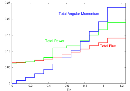
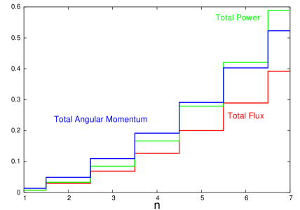
Figure 12: Total emissivities for scalar emission on the brane from a rotating black hole as a function of (a) $a_{*}$, for $n=4$, and (b) $n$ for $a_{*}=1$.

The dependence of the total emissivities on the dimensionality of spacetime is shown in the second histogram shown in Fig. 12(b), that clearly illustrates the enhancement of all fluxes as $n$ increases. For $a_{*}$ fixed ($a_{*}=1$) and $n$ varying from 1 to 7, the number of particles emitted by the black hole on the brane per unit time is enhanced by a factor of 30, the energy flux by a factor of 100, and the angular momentum flux by a factor of 40.

A note should be made at this point: the results presented above are only an approximation to the exact, total emissivities that would follow by integrating the various fluxes over the complete frequency regime. In this work, numerical results have been produced only up to the frequency value of $\omega r_{h}=3$ as the integration for higher values of $\omega r_{h}$ takes an unrealistically long time. For small values of $n$ and $a_{*}$, the flux dies away sufficiently quickly, therefore the contribution from $\omega r_{h}>3$ is negligible and the derived emissivities are an adequate approximation to the actual ones. However, as the value of either $a_{*}$ or $n$ increases, the peak of the Gaussian curve moves to higher energies, and the contribution of the part of the spectrum that we are missing to the exact emissivities is increasing. Nevertheless, the graphs presented in this subsection accurately describe the correct qualitative behaviour of the exact emissivities: the part of the spectrum that has been left out of our calculation would only increase further the enhancement of all three fluxes if it could be taken into account.

We have also computed the integral over the frequency of the angular distribution of the particle flux (28) and power spectrum (29) to derive the emissivity solely as a function of the azimuthal angle $\theta$. In Figs. 13(a,b), we depict the power emissivity as a function of $\cos\theta$ for fixed $n$ and variable $a_{*}$, and vice versa – the flux emissivity exhibits a similar behaviour and therefore is not shown here. The behaviour found agrees with the one deduced from the 3D graphs of subsections 4.1 and 4.2. For fixed $n$, as the angular momentum parameter $a_{*}$ increases, the energy (and particle) flux is altogether enhanced and becomes more concentrated around the equatorial region; for fixed $a_{*}$, the fluxes strongly increase as $n$ increases, and so does again the proportion of the emission concentrated in the equatorial region.

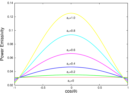
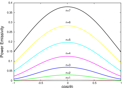
Figure 13: Power emissivity for scalar emission on the brane from a rotating black hole as a function of $\cos\theta$, (a) for $n=4$ and variable $a_{*}$, and (b) for $a_{*}=1$ and variable $n$.

5 Discussion and Conclusions

In this work we have performed a comprehensive analysis of the emission of Hawking radiation in the form of scalar fields from a $(4+n)$-dimensional, rotating black hole on the brane. This analysis has provided complete results for the flux, energy and angular momentum spectra for the spin-down phase of the life of a higher-dimensional black hole, thus, filling a long-standing gap in the literature. By means of numerical analysis, we have been able to solve both the radial and angular equations for the scalar field modes, and our method is applicable for arbitrary energy of the emitted particles, angular momentum of the black hole, and number of extra, spacelike dimensions.

We have first studied the fluxes of scalar particles, energy and angular momentum – integrated over the azimuthal angle $\theta$ – for a range of values of the angular momentum of the black hole $a_{*}$ and number of extra dimensions $n$, in each case as a function of the mode frequency $\omega$. Due to their relation, a number of common features arise between the flux and power spectra: for low values of $n$, both emission rates are suppressed at the low energy regime but strongly enhanced in the intermediate- and high-energy one, as the angular momentum parameter increases; for high values of $n$, the enhancement is present at all frequency regimes. On the other hand, the rate of loss of the angular momentum of the black hole increases uniformly (i.e. at all frequency regimes) as $a_{*}$ increases, for all values of $n$. When the angular momentum parameter is kept fixed and $n$ increases, a clear, strong enhancement can be seen in all three spectra and in all frequency regimes. This enhancement can be easily explained by the fact that, for fixed $a_{*}$, as $n$ increases, the temperature of the black hole, given by Eq. (17), increases too, thus leading to greater emission rates. However, for fixed $n$, increasing $a_{*}$ lowers the temperature, and, in this case, the increased emission rates is due to enhanced super-radiance, which speeds up the spin-down process.

We have also considered the angular distribution of the particle and energy fluxes. Again, a number of common features arise in the two spectra. An important feature is the dominance of the spherically-symmetric emission at the low-energy regime that leads to an almost $\theta$-independent distribution even for a non-vanishing angular momentum parameter; as the energy of the emitted particles increases, however, a clear angular dependence – that is, the concentration of the emitted modes near the equatorial plane – appears in both spectra. We expect the angular variation in the emission rates to be a unique feature of the spectra during the spin-down phase.

All spectra derived above, either integrated or not over the $\theta$-coordinate, depend strongly on the energy regime that we look at, the value of the angular momentum parameter and the dimensionality of spacetime. In many cases, the various emission rates change considerably as the above parameters take different, low or high, values. In this work, care has been taken so that all relevant quantities, i.e. the angular eigenvalue as well as the radial and angular part of the scalar field, are computed via numerical analysis that is free from any assumptions and approximations that limit the values of the aforementioned three, fundamental parameters of the problem.

Any assumptions made in this analysis involved only the mass of the produced black hole, being much larger than the fundamental Planck mass, and the size of the horizon of the black hole, being much smaller than the size of the extra dimensions. However, the values of $M_{*}$ and $L$ themselves were never specified; they are free input parameters of the problem, and thus our analysis and corresponding results are valid for any gravitational theory with arbitrary number of extra dimensions and fundamental scale. Finally, although our analysis assumed that the extra spacetime is empty and thus flat, our results are also valid in the case of a Randall-Sundrum [40] type of black hole in the limit of a horizon radius being much smaller than the AdS radius.

A number of interesting questions still remain open. Firstly, the calculation of the rate of spin-down of the black hole [41], and thus of the duration of this phase compared to the Schwarzschild one, requires, in addition to the brane emission, the scalar field radiation into the bulk for all values of the number of extra dimensions. The same calculation for the flux and energy spectra will reveal the amount of energy lost in the bulk and thus the remaining amount available for emission on the brane. Also, the remaining brane emission ‘channels’, i.e. the ones for fermions and gauge bosons, need to be investigated too. It is thus necessary, and of great interest indeed, to extend our analysis for the emission of Hawking radiation from a rotating, higher-dimensional black hole for higher-spin particles. We plan to return to these questions in the near future.

Acknowledgments. We would like to thank Marc Casals for helpful discussions. E.W. would like to thank the following for hospitality while this work was completed: the Institute for Particle Physics Phenomenology, University of Durham; the Department of Mathematical Physics, University College Dublin; and the School of Mathematics and Statistics, University of Newcastle-upon-Tyne. The work of P.K. was funded by the UK PPARC Research Grant PPA/A/S/2002/00350. The work of E.W. is supported by UK PPARC, grant reference number PPA/G/S/2003/00082, the Royal Society and the London Mathematical Society.

References

-
[1]
N. Arkani-Hamed, S. Dimopoulos and G. R. Dvali,
Phys. Lett. B 429, 263 (1998) [hep-ph/9803315];
Phys. Rev. D 59, 086004 (1999) [hep-ph/9807344];
I. Antoniadis, N. Arkani-Hamed, S. Dimopoulos and G. R. Dvali, Phys. Lett. B 436, 257 (1998) [hep-ph/9804398]. -
[2]
K. Akama,
Lect. Notes Phys. 176, 267 (1982) [hep-th/0001113];
V. A. Rubakov and M. E. Shaposhnikov, Phys. Lett. B 125, 139 (1983); Phys. Lett. B 125, 136 (1983);
M. Visser, Phys. Lett. B 159, 22 (1985) [hep-th/9910093];
G. W. Gibbons and D. L. Wiltshire, Nucl. Phys. B287, 717 (1987);
I. Antoniadis, Phys. Lett. B 246, 377 (1990);
I. Antoniadis, K. Benakli and M. Quiros, Phys. Lett. B 331, 313 (1994) [hep-ph/9403290];
J. D. Lykken, Phys. Rev. D 54, 3693 (1996) [hep-th/9603133]. -
[3]
T. Banks and W. Fischler,
hep-th/9906038;
D. M. Eardley and S. B. Giddings, Phys. Rev. D 66, 044011 (2002) [gr-qc/0201034];
H. Yoshino and Y. Nambu, Phys. Rev. D 66, 065004 (2002) [gr-qc/0204060]; Phys. Rev. D 67, 024009 (2003) [gr-qc/0209003];
E. Kohlprath and G. Veneziano, JHEP 0206, 057 (2002) [gr-qc/0203093];
V. Cardoso, O. J. C. Dias and J. P. S. Lemos, Phys. Rev. D 67, 064026 (2003) [hep-th/0212168];
E. Berti, M. Cavaglia and L. Gualtieri, Phys. Rev. D 69, 124011 (2004) [hep-th/ 0309203];
L. A. Anchordoqui, J. L. Feng, H. Goldberg and A. D. Shapere, Phys. Lett. B 594, 363 (2004) [hep-ph/0311365];
V. S. Rychkov, Phys. Rev. D 70, 044003 (2004) [hep-ph/0401116];
S. B. Giddings and V. S. Rychkov, Phys. Rev. D 70, 104026 (2004) [hep-th/0409131];
O. I. Vasilenko, hep-th/0305067; hep-th/0407092;
H. Yoshino and V. S. Rychkov, Phys. Rev. D 71, 104028 (2005) [hep-th/0503171];
V. Cardoso, E. Berti and M. Cavaglia, Class. Quant. Grav. 22, L61 (2005) [hep-ph/0505125]. -
[4]
P. C. Argyres, S. Dimopoulos and J. March-Russell,
Phys. Lett. B 441, 96 (1998) [hep-th/9808138];
R. Emparan, G. T. Horowitz and R. C. Myers, Phys. Rev. Lett. 85, 499 (2000) [hep-th/0003118];
S. B. Giddings and S. Thomas, Phys. Rev. D 65, 056010 (2002) [hep-ph/0106219];
S. Dimopoulos and G. Landsberg, Phys. Rev. Lett. 87, 161602 (2001) [hep-ph/0106295];
S. Dimopoulos and R. Emparan, Phys. Lett. B 526, 393 (2002) [hep-ph/0108060];
S. Hossenfelder, S. Hofmann, M. Bleicher and H. Stocker, Phys. Rev. D 66, 101502 (2002) [hep-ph/0109085];
K. Cheung, Phys. Rev. Lett. 88, 221602 (2002) [hep-ph/0110163];
R. Casadio and B. Harms, Int. J. Mod. Phys. A 17, 4635 (2002) [hep-ph/0110255];
S. C. Park and H. S. Song, J. Korean Phys. Soc. 43, 30 (2003) [hep-ph/0111069];
G. Landsberg, Phys. Rev. Lett. 88, 181801 (2002) [hep-ph/0112061];
G. F. Giudice, R. Rattazzi and J. D. Wells, Nucl. Phys. B 630, 293 (2002) [hep-ph/0112161];
E. J. Ahn, M. Cavaglia and A. V. Olinto, Phys. Lett. B 551, 1 (2003) [hep-th/0201042];
T. G. Rizzo, JHEP 0202, 011 (2002) [hep-ph/0201228]; hep-ph/0412087;
A. V. Kotwal and C. Hays, Phys. Rev. D 66, 116005 (2002) [hep-ph/0206055];
A. Chamblin and G. C. Nayak, Phys. Rev. D 66, 091901 (2002) [hep-ph/0206060];
T. Han, G. D. Kribs and B. McElrath, Phys. Rev. Lett. 90, 031601 (2003) [hep-ph/0207003];
I. Mocioiu, Y. Nara and I. Sarcevic, Phys. Lett. B 557, 87 (2003) [hep-ph/0310073];
M. Cavaglia, S. Das and R. Maartens, Class. Quant. Grav. 20, L205 (2003) [hep-ph/0305223];
C. M. Harris, P. Richardson and B. R. Webber, JHEP 0308, 033 (2003) [hep-ph/0307305];
R. A. Konoplya, Phys. Rev. D 68, 124017 (2003) [hep-th/0309030]; Phys. Rev. D 71, 024038 (2005) [hep-th/0410057];
V. Cardoso, J. P. S. Lemos and S. Yoshida, Phys. Rev. D 69, 044004 (2004) [gr-qc/0309112];
M. Cavaglia and S. Das, Class. Quant. Grav. 21, 4511 (2004) [hep-th/0404050];
D. Stojkovic, Phys. Rev. Lett. 94, 011603 (2005) [hep-ph/0409124];
S. Hossenfelder, Mod. Phys. Lett. A 19, 2727 (2004) [hep-ph/0410122];
C. M. Harris, M. J. Palmer, M. A. Parker, P. Richardson, A. Sabetfakhri and B. R. Webber, hep-ph/0411022;
T. G. Rizzo, JHEP 0501, 028 (2005) [hep-ph/0412087]; JHEP 0506, 079 (2005) [hep-ph/0503163];
J. L. Hewett, B. Lillie and T. G. Rizzo, hep-ph/0503178;
L. Lonnblad, M. Sjodahl and T. Akesson, hep-ph/0505181;
B. Koch, M. Bleicher and S. Hossenfelder, hep-ph/0507138; hep-ph/0507140. -
[5]
A. Goyal, A. Gupta and N. Mahajan,
Phys. Rev. D 63, 043003 (2001) [hep-ph/0005030];
J. L. Feng and A. D. Shapere, Phys. Rev. Lett. 88, 021303 (2002) [hep-ph/0109106];
L. Anchordoqui and H. Goldberg, Phys. Rev. D 65, 047502 (2002) [hep-ph/0109242];
R. Emparan, M. Masip and R. Rattazzi, Phys. Rev. D 65, 064023 (2002) [hep-ph/ 0109287];
L. A. Anchordoqui, J. L. Feng, H. Goldberg and A. D. Shapere, Phys. Rev. D 65, 124027 (2002) [hep-ph/0112247]; Phys. Rev. D 68, 104025 (2003) [hep-ph/0307228];
Y. Uehara, Prog. Theor. Phys. 107, 621 (2002) [hep-ph/0110382];
J. Alvarez-Muniz, J. L. Feng, F. Halzen, T. Han and D. Hooper, Phys. Rev. D 65, 124015 (2002) [hep-ph/0202081];
A. Ringwald and H. Tu, Phys. Lett. B 525, 135 (2002) [hep-ph/0111042];
M. Kowalski, A. Ringwald and H. Tu, Phys. Lett. B 529, 1 (2002) [hep-ph/0111042];
E. J. Ahn, M. Ave, M. Cavaglia and A. V. Olinto, Phys. Rev. D 68, 043004 (2003) [hep-ph/0306008];
E. J. Ahn, M. Cavaglia and A. V. Olinto, Astropart. Phys. 22, 377 (2005) [hep-ph/0312249];
T. Han and D. Hooper, New J. Phys. 6, 150 (2004) [hep-ph/0408348];
A. Cafarella, C. Coriano and T. N. Tomaras, hep-ph/0410358;
A. Barrau, C. Feron and J. Grain, astro-ph/0505436. - [6] P. Kanti, Int. J. Mod. Phys. A 19, 4899 (2004) [hep-ph/0402168].
-
[7]
M. Cavaglia,
Int. J. Mod. Phys. A 18, 1843 (2003) [hep-ph/0210296];
G. Landsberg, Eur. Phys. J. C 33, S927 (2004) [hep-ex/0310034];
K. Cheung, hep-ph/0409028;
S. Hossenfelder, hep-ph/0412265;
A. S. Majumdar and N. Mukherjee, astro-ph/0503473. - [8] C. M. Harris, hep-ph/0502005.
- [9] P. Kanti and J. March-Russell, Phys. Rev. D 66, 024023 (2002) [hep-ph/0203223].
- [10] V. P. Frolov and D. Stojkovic, Phys. Rev. D 66, 084002 (2002) [hep-th/0206046].
- [11] P. Kanti and J. March-Russell, Phys. Rev. D 67, 104019 (2003) [hep-ph/0212199].
- [12] C. M. Harris and P. Kanti, JHEP 0310, 014 (2003) [hep-ph/0309054].
- [13] A. Barrau, J. Grain and S. O. Alexeyev, Phys. Lett. B 584, 114 (2004).
- [14] E. l. Jung, S. H. Kim and D. K. Park, Phys. Lett. B 586, 390 (2004) [hep-th/0311036]; JHEP 0409, 005 (2004) [hep-th/0406117]; Phys. Lett. B 602, 105 (2004) [hep-th/0409145].
- [15] M. Doran and J. Jaeckel, astro-ph/0501437.
-
[16]
E. Jung and D. K. Park,
Nucl. Phys. B 717, 272 (2005) [hep-th/0502002];
E. Jung, S. Kim and D. K. Park, Phys. Lett. B 614, 78 (2005) [hep-th/0503027]. - [17] P. Kanti, J. Grain and A. Barrau, Phys. Rev. D 71, 104002 (2005) [hep-th/0501148].
- [18] V. P. Frolov and D. Stojkovic, Phys. Rev. D 67, 084004 (2003) [gr-qc/0211055].
- [19] D. Ida, K. y. Oda and S. C. Park, Phys. Rev. D 67, 064025 (2003), Erratum-ibid. D 69, 049901 (2004) [hep-th/0212108].
- [20] C. M. Harris and P. Kanti, hep-th/0503010.
- [21] D. Ida, K. y. Oda and S. C. Park, hep-ph/0501210.
- [22] E. Jung, S. Kim and D. K. Park, Phys. Lett. B 615, 273 (2005) [hep-th/0503163]; hep-th/0504139.
- [23] D. Ida, K. y. Oda and S. C. Park, Phys. Rev. D 71, 124039 (2005) [hep-th/0503052].
- [24] H. Nomura, S. Yoshida, M. Tanabe and K. i. Maeda, hep-th/0502179.
- [25] E. Jung and D. K. Park, hep-th/0506204.
- [26] M. Casals, P. Kanti and E. Winstanley, in progress.
- [27] R. C. Myers and M. J. Perry, Annals Phys. 172, 304 (1986).
- [28] S. W. Hawking, Commun. Math. Phys. 43, 199 (1975).
-
[29]
W. T. Zaumen, Nature 247, 530 (1974);
B. Carter, Phys. Rev. Lett. 33, 558 (1974);
A. A. Starobinskii and S. M. Churilov, Sov. Phys.-JETP 38, 1 (1974);
G. W. Gibbons, Commun. Math. Phys. 44, 245 (1975);
W. G. Unruh, Phys. Rev. D 14, 3251 (1976). - [30] D. N. Page, Phys. Rev. D 13, 198 (1976); Phys. Rev. D 14, 1509 (1976); Phys. Rev. D 14, 3260 (1976); Phys. Rev. D 16, 2402 (1977).
- [31] N. Sanchez, Phys. Rev. D 16, 937 (1977); Phys. Rev. D 18, 1030 (1978); Phys. Rev. D 18, 1798 (1978).
-
[32]
M. Abramowitz and I. A. Stegun, Handbook of Mathematical Functions
(Dover, New York, 1964);
C. Flammer, Spheroidal wave functions (Stanford University Press, 1957);
J. N. Goldberg, A. J. MacFarlane, E. T. Newman, F. Rohrlich and E. C. Sudarshan, J. Math. Phys. 8, 2155 (1967);
J. Meixner, F. W. Schäfke, and G. Wolf, Mathieu functions and spheroidal functions and their mathematical foundations, further studies (Springer-Verlag, Berlin, 1980);
E. Seidel, Class. Quant. Grav. 6, 1057 (1989). - [33] A. C. Ottewill and E. Winstanley, Phys. Rev. D 62, 084018 (2000) [gr-qc/0004022].
- [34] V. P. Frolov and K. S. Thorne, Phys. Rev. D 39, 2125 (1989).
-
[35]
G. Duffy, PhD thesis, University College Dublin (2002).
G. Duffy and A. C. Ottewill, to appear. - [36] E. Wasserstrom, J. Comp. Phys. 9, 53 (1972).
- [37] W. H. Press, S. A. Teukolsky, W. T. Vetterling and B. P. Flannery, Numerical Recipes in Fortran (Cambridge University Press, 1986).
- [38] M. Casals and A. C. Ottewill, Phys. Rev. D 71, 064025 (2005) [gr-qc/0409012].
- [39] E. W. Leaver, Proc. Roy. Soc. London A 402, 285 (1985).
- [40] L. Randall and R. Sundrum, Phys. Rev. Lett. 83, 3370 (1999) [hep-ph/9905221]; Phys. Rev. Lett. 83, 4690 (1999) [hep-ph/9906064].
- [41] C. M. Chambers, W. A. Hiscock and B. Taylor, Phys. Rev. Lett. 78, 3249 (1997) [gr-qc/9703018].