CALT-68-2568

ITEP-TH-50/05

Bäcklund transformations, energy shift
and the plane wave limit.



Andrei Mikhailov

California Institute of Technology 452-48, Pasadena CA 91125

and

Institute for Theoretical and Experimental Physics,
117259, Bol. Cheremushkinskaya, 25, Moscow, Russia

We discuss basic properties of the Bäcklund transformations for the classical string in AdS space in the context of the null-surface perturbation theory. We explain the relation between the Bäcklund transformations and the energy shift of the dual field theory state. We show that the Bäcklund transformations can be represented as a finite-time evolution generated by a special linear combination of the Pohlmeyer charges. This is a manifestation of the general property of Bäcklund transformations known as spectrality. We also discuss the plane wave limit.

1 Introduction

One of the main goals of the AdS/CFT correspondence is to gain insight in the dynamics of the string theory in backgrounds with nonzero Ramond-Ramond field strength. Integrability is important in the AdS/CFT program [1, 2, 3, 4]. Our understanding of classical integrability of the string worldsheet is probably somewhat incomplete at this point, but even the current results are already very impressive. Many explicit solutions are known, and in some sense we have the full construction of the action-angle variables in the finite-gap approach [5, 6, 7, 8, 9]. There is a remarkable partial agreement with the Yang-Mills perturbative calculations of the anomalous dimension [10, 11, 12, 13].

The most important goal in the classical theory of integrability is to identify the integrable structures which have a transparent meaning in the quantum theory. In the integrable string theory, we eventually want to be able to generalize the integrable structures from the sphere to the higher genus surfaces. From this point of view, it would be useful to understand the integrability as much as possible in terms of the objects which are local on the worldsheet. This would be also important if we want to compare the string theory computations to the Yang-Mills computations, because the Yang-Mills diagramms are local in a sense that they involve only the interactions of those partons which are close neighbors on the spin chain.

Examples of those objects which are local on the worldsheet are local conserved charges and Bäcklund equations. Local conserved charges were constructed by Pohlmeyer, and in fact Bäcklund transformations were used to define them [14] and to actually compute them for particular solutions [15]. Bäcklund transformations allow us to construct the new solution from a given solution, as a solution of the differential equation which we will call the Bäcklund equation. The Bäcklund equation depends on the real parameter $\gamma$. It is of the form

$$\partial\phi_{new}=\Phi_{\gamma}(\phi_{new},\phi_{old},\partial\phi_{old})$$ (1)

where $\phi$ are the embedding functions of the string worldsheet into the target space and $\partial$ stands for the derivatives with respect to the worldsheet coordinates. Solving the Bäcklund equation involves the choice of the integration constants. It turns out that for some particular value of the integration constants $\phi_{new}$ is in fact a Hamiltonian flow of $\phi_{old}$ by a certain infinite linear combination of the local conserved charges. The coefficients of this infinite linear combination depend on $\gamma$. For every $\gamma$ we have a Hamiltonian $H_{\gamma}$ and the corresponding Hamiltonian vector field $\xi_{\gamma}$ such that the flow by the finite time is the Bäcklund transformation. This means that, even though the local conserved charges can appear to be complicated in form, in fact the Hamiltonian flows generated by certain combinations of these charges by a finite time are controlled by the explicitly known differential equation of the form (1) which is in fact closely related to the auxiliary linear problem.

Bäcklund transformations are important in the quantum theory [17, 18, 19]. The Hamiltonian is usually related to the quantum Bäcklund transformation by the Baxter’s $T-Q$ relation. In the context of AdS/CFT correspondence the natural object is not the Hamiltonian (which would not be conformally invariant) but the discrete “deck transformation” which corresponds to the anomalous dimension on the Yang-Mills side (see the discussion in Section 2.3.1 and in [21]). As we will see in the Section 2.3.2, the deck transformation is literally a particular example of a Bäcklund transformation. It would be very interesting to see if there is an analogue of this fact for the Yang-Mills diagramms.

In Section 2 we discuss the basic properties of Bäcklund transformations, prove their canonicity and explain the relation between Bäcklund transformations and deck transformations. We also argue that a Bäcklund transformation can be represented as a Hamiltonian flow by a finite time generated by an infinite linear combination of the local conserved charges. (We will call this infinite linear combination the “generator” of the Bäcklund transformation.) Some of the results of Section 2 have already been presented in [21, 25]. In Section 3 we derive the explicit formula (64), (65) for the generator. We present two methods of deriving this formula: using the plane wave limit and using the formula (21) for the variation of the symplectic potential under the Bäcklund transformation. We also use the results of [26] to express the formula (55) for the anomalous dimension conjectured in [27] in terms of the eigenvalues of the monodromy matrix. We use the properties of Bäcklund transformation to prove this conjectured formula.

We use the plane wave limit of the local conserved charges and Bäcklund transformations. This limit has a clear physical meaning explained in [28]. In this limit the string worldsheet theory becomes the theory of free massive fields. Although this is just a limit, in some sense it “captures” all the conserved charges, at least the local charges. Therefore we can use the plane wave limit to guess, and even prove, various relations between the conserved charges which hold beyond this limit.

2 Anomalous dimension as a Bäcklund transformation.

2.1 Deviation of the string worldsheet from being periodic.

An important property of the AdS space is its “periodicity”. It is often convenient to introduce the global coordinates in which the metric becomes:

$$ds^{2}=-(1+r^{2})dt^{2}+{dr^{2}\over 1+r^{2}}+r^{2}d\Omega_{S^{n-1}}^{2}$$

In these coordinates the periodicity corresponds to the discrete symmetry $t\to t+2\pi$. It is important that this discrete symmetry commutes with all the global symmetries and in fact belongs to the center of $SO(2,n)$. We will call it “deck transformation”, because it is a deck transformation if we think of $AdS_{n+1}$ as the universal covering space of the hyperboloid.

Consider the Type IIB superstring theory on $AdS_{5}\times S^{5}$. It is useful to look at the deviation of the dynamics of the theory from being periodic in $t$. For example, solutions of the linearized classical supergravity equations are exactly periodic (invariant under $t\mapsto t+2\pi$), although the solutions of the nonlinear classical supergravity are generally speaking not periodic. Consider a classical string moving in $AdS_{5}\times S^{5}$. If we neglect the backreaction of the string on the AdS geometry, then it is possible to quantitatively characterize the deviation of the string worldsheet from being periodic in $t$.

Indeed, the transformation $t\mapsto t+2\pi$ is a discrete symmetry and we can ask ourselves how it acts on the string phase space. The classical superstring on $AdS_{5}\times S^{5}$ is an integrable model, there are infinitely many conserved charges in involution. In some sense these charges generate the “invariant tori”. This is precisely true for the so-called finite-gap solutions. The Hamiltonian flows of these finite-gap solutions fill the finite-dimensional tori. (For the general solutions we can probably talk about the “infinite-dimensional tori” but it is not very clear what these words mean.) If we represent the invariant torus as a quotient

$${\bf T}^{g}={\bf R}^{g}/({\bf Z}e_{1}+\ldots+{\bf Z}e_{g})$$

then the transformation $t\mapsto t+2\pi$ would act as a shift by the vector $a_{1}e_{1}+\ldots+a_{g}e_{g}$. The numbers $a_{1},\ldots,a_{g}$ characterize quantitatively the deviation of the string worldsheet from being periodic in $t$.

The set of points ${\bf Z}(a_{1}e_{1}+\ldots+a_{g}e_{g})$ is usually a dense subset of the invariant torus, and therefore it actually defines the torus (the torus is the “closure” of this set). This suggests that the action of this discrete symmetry carries a lot of information about the dynamics of the string. On the field theory side this symmetry measures the anomalous dimension of the corresponding CFT operator.

2.2 Bäcklund transformations.

2.2.1 Definition of Bäcklund transformations.

The classical string is the nonlinear sigma-model with the Virasoro constrains. Most of the discussion in our paper is valid independently of the Virasoro constraints. If we turn off the fermions, the nonlinear sigma-model on $AdS_{5}\times S^{5}$ is essentially the product of the sigma-models on $AdS_{5}$ and $S^{5}$. We will concentrate on the $AdS_{5}$-part of the sigma-model. Let us parametrize the points on $AdS_{5}/{\bf Z}$ by the unit vectors $X^{\mu}$, $\mu\in{-1,0,1,2,3,4}$, subject to the constraint $g_{\mu\nu}X^{\mu}X^{\nu}=1$ with $g_{\mu\nu}=\mbox{diag}(1,1,-1,-1,-1,-1)$. This means that we realize $AdS_{5}/{\bf Z}$ as the hyperboloid in ${\bf R}^{2+4}$. In this subsection we will consider the Bäcklund transformations acting on the projection of the string worldsheet to the hyperboloid $AdS_{5}/{\bf Z}$. We will consider the lift of the Bäcklund transformations to the string on $AdS_{5}$ in Section 2.3.2.

There are infinitely many Pohlmeyer charges ${\cal F}_{2n}$ and $\widetilde{\cal F}_{2n}$ introduced in [14] and the corresponding Hamiltonian vector fields will be denoted $\xi_{{\cal F}_{2n}}$ and $\xi_{\widetilde{\cal F}_{2n}}$. We will give a definition of the Pohlmeyer charges in Section 3.1, but here we just point out that they are the local conserved charges. A local conserved charge is given by an integral over the closed contour on the string worldsheet of a closed differential 1-form, which is constructed from the worldsheet fields $X(\tau,\sigma)$ and their derivatives. The integral does not depend on the choice of the contour because the 1-form is closed. In this sense, it is a conserved charge. The existence of infinitely many closed differential 1-forms on the worldsheet is a very nontrivial fact related to the integrability of the worldsheet theory.

Given a vector field $\xi$ on the phase space we can consider the flow of this vector field. It is a one-parameter family of transformations which we will denote:

$$e^{s\xi}\;\;\mbox{or}\;\;\exp(s\xi)$$

Given a point $x$ of the phase space, the flow by the time $s$ of this point, denoted $e^{s\xi}x$, is defined as $y(s)$ where $y(t)$ is the solution of the differential equation ${dy(t)\over dt}=\xi(y(t))$ with the initial condition $y(0)=x$.

We introduce the conformal coordinates $\tau$ and $\sigma$ on the worldsheet so that the metric is proportional to $d\tau^{2}-d\sigma^{2}$. We denote $\partial_{\pm}={1\over 2}(\partial_{\tau}\pm\partial_{\sigma})$. Given the string worldsheet $X^{\mu}(\tau,\sigma)$ we consider two discrete transformations $B_{\gamma}X$ and $\tilde{B}_{\tilde{\gamma}}X$ depending on real parameters $\gamma$ and $\tilde{\gamma}$, which are defined by the following properties:

1. These transformations are generated by the Hamiltonian flows of the Pohlmeyer charges:

   $$B_{\gamma}X=\exp\left(\sum_{n}t_{2n}({\gamma})\xi_{{\cal F}_{2n}}\right).X$$ (2)

   $$\tilde{B}_{\tilde{\gamma}}X=\exp\left(\sum_{n}\tilde{t}_{2n}(\tilde{\gamma})\xi_{\widetilde{\cal F}_{2n}}\right).X$$ (3)

   with some coefficients $t_{2n}$ and $\tilde{t}_{2n}$ depending on $\gamma$ and $\tilde{\gamma}$.

2. They satisfy the following first order differential equations:

   $$\begin{array}[]{l}\partial_{-}(B_{\gamma}X-X)=-{1\over 2}(1+\gamma^{2})(B_{\gamma}X,\partial_{-}X)(B_{\gamma}X+X)\\[5.0pt] \partial_{+}(B_{\gamma}X+X)={1\over 2}(1+\gamma^{-2})(B_{\gamma}X,\partial_{+}X)(B_{\gamma}X-X)\end{array}$$ (4)

   $$\begin{array}[]{l}\partial_{+}(\tilde{B}_{\tilde{\gamma}}X-X)=-{1\over 2}(1+\tilde{\gamma}^{-2})(\tilde{B}_{\tilde{\gamma}}X,\partial_{+}X)(\tilde{B}_{\tilde{\gamma}}X+X)\\[5.0pt] \partial_{-}(\tilde{B}_{\tilde{\gamma}}X+X)={1\over 2}(1+\tilde{\gamma}^{2})(\tilde{B}_{\tilde{\gamma}}X,\partial_{-}X)(\tilde{B}_{\tilde{\gamma}}X-X)\end{array}$$ (5)

3. For small $\gamma$ and large $\tilde{\gamma}$:

   $$B_{\gamma}X=X-\gamma{\partial_{+}X\over|\partial_{+}X|}+o(\gamma)$$ (6)

   $$\tilde{B}_{\tilde{\gamma}}X=X+{1\over\tilde{\gamma}}{\partial_{-}X\over|\partial_{-}X|}+o\left({1\over\tilde{\gamma}}\right)$$ (7)

We conjecture that the transformations $B_{\gamma}$ and $\tilde{B}_{\tilde{\gamma}}$ exist and are determined unambiguously by these three properties, at least if the velocity of the string is large enough. The coefficients $t_{n}(\gamma)$ and $\tilde{t}_{n}(\tilde{\gamma})$ will be determined in Section 3. The relation between Bäcklund transformations and the Hamiltonian vector fields generated by the local conserved charges in the special case when the motion of the string is restricted to ${\bf R}\times S^{2}$ was discussed in [25].

2.2.2 Perturbative solutions of Bäcklund equations.

Eqs. (4), (5), (6) and (7) can be solved as the series in $\gamma$ and $1/\tilde{\gamma}$ when $\gamma$ is small and $\tilde{\gamma}$ is large. The recurrent relations allowing to construct the solution order by order in $\gamma$ and $1/\tilde{\gamma}$ were written for example in [15].

Another way of solving (4) and (5) perturbatively is to use the null-surface perturbation theory [30, 31, 32, 33, 34] with the small parameter $1/|\partial_{\tau}X|$. (More precisely, the small parameter is the angle between $\partial_{+}X$ and $\partial_{-}X$; in the null-surface limit $\partial_{+}X=\partial_{-}X$. If we define the conformal coordinates $(\tau,\sigma)$ so that $|\partial_{\sigma}X|\simeq 1$ then the small parameter is $1/|\partial_{\tau}X|$. Alternatively, if we define the coordinates so that $|\partial_{\tau}X|\simeq 1$, then the small parameter is $|\partial_{\sigma}X|$.) The zeroth order is:

$$B_{\gamma}X={1-\gamma^{2}\over 1+\gamma^{2}}X-{2\gamma\over 1+\gamma^{2}}{\partial_{\tau}X\over|\partial_{\tau}X|}+\ldots$$ (8)

$$\tilde{B}_{\tilde{\gamma}}X={1-\tilde{\gamma}^{-2}\over 1+\tilde{\gamma}^{-2}}X+{2\tilde{\gamma}^{-1}\over 1+\tilde{\gamma}^{-2}}{\partial_{\tau}X\over|\partial_{\tau}X|}+\ldots$$ (9)

where dots denote the terms of the higher order in $1/|\partial_{\tau}X|$. We believe that the series of the null-surface perturbation theory converge if the string moves fast enough, but we do not have a proof of that.

The null-surface perturbation theory works for finite values of $\gamma$ and $\tilde{\gamma}$. But if $\gamma$ is small, then the null-surface perturbation theory agrees with the perturbative expansion in $\gamma$, in the following sense. Any finite order of the null-surface expansion is a rational function of $\gamma$, and can be expanded as a Taylor series around $\gamma=0$. These series in $\gamma$ converge in some finite region of the parameter $\gamma$ around $\gamma=0$. We will now discuss some details of the null-surface perturbation theory for $B_{\gamma}X$ and explain why any finite order is a rational function of $\gamma$.

Suppose that $1/M$ is a small parameter of the null-surface perturbation theory, and choose the coordinates $\tau$, $\sigma$ so that:

$$|\partial_{\tau}X|\simeq 1,\;\;\;|\partial_{\sigma}X|\simeq 1/M$$

We can introduce the new worldsheet coordinate $s=\sigma/M$ so that $|\partial_{s}X|\simeq 1$ and $\partial_{\pm}={1\over 2}(\partial_{\tau}\pm M^{-1}\partial_{s})$. Subtracting the first equation of (4) from the second equation of (4) we get

$$B_{\gamma}X-{1-\gamma^{2}\over 1+\gamma^{2}}X-{4\partial_{\tau}X\over(\gamma+\gamma^{-1})^{2}(B_{\gamma}X,\partial_{\tau}X)}={M^{-1}\Phi[X,B_{\gamma}X]\over(\gamma+\gamma^{-1})^{2}(B_{\gamma}X,\partial_{\tau}X)}$$ (10)

where

$$\Phi[X,B_{\gamma}X]=4\partial_{s}B_{\gamma}X+(\gamma^{2}-\gamma^{-2})(B_{\gamma}X,\partial_{s}X)B_{\gamma}X+(\gamma+\gamma^{-1})^{2}(B_{\gamma}X,\partial_{s}X)X$$

The null-surface perturbation theory can be understood as solving Eq. (10) for $B_{\gamma}X$ by an iterative procedure, taking as the zeroth order ($M=\infty$): $B_{\gamma}^{(0)}X={1-\gamma^{2}\over 1+\gamma^{2}}X-{2\gamma\over 1+\gamma^{2}}{\partial_{\tau}X\over|\partial_{\tau}X|}$. Given $B_{\gamma}^{(n)}$, we define $B_{\gamma}^{(n+1)}$ by the formula

$$B_{\gamma}^{(n+1)}X-{1-\gamma^{2}\over 1+\gamma^{2}}X-{4\partial_{\tau}X\over(\gamma+\gamma^{-1})^{2}(B^{(n+1)}_{\gamma}X,\partial_{\tau}X)}={M^{-1}\Phi[X,B^{(n)}_{\gamma}X]\over(\gamma+\gamma^{-1})^{2}(B^{(n)}_{\gamma}X,\partial_{\tau}X)}$$

This equation defines $B^{(n+1)}_{\gamma}X$ in terms of $X$ and $B^{(n)}_{\gamma}X$ in the following way. We represent $B^{(n+1)}_{\gamma}X=(B^{(n+1)}_{\gamma}X)_{\perp}+S^{(n+1)}_{\gamma}{\partial_{\tau}X\over|\partial_{\tau}X|^{2}}$, where

$$(B^{(n+1)}_{\gamma}X)_{\perp}={1-\gamma^{2}\over 1+\gamma^{2}}X+\left[{M^{-1}\Phi[X,B^{(n)}_{\gamma}X]\over(\gamma+\gamma^{-1})^{2}(B^{(n)}_{\gamma}X,\partial_{\tau}X)}\right]_{\perp}$$

the subindex $\perp$ meaning the component of the vector orthogonal to $\partial_{\tau}X$, and $S^{(n+1)}_{\gamma}=(B^{(n+1)}_{\gamma}X,\partial_{\tau}X)$ is determined from the quadratic equation:

$$S^{(n+1)}_{\gamma}-{4|\partial_{\tau}X|^{2}\over(\gamma+\gamma^{-1})^{2}S^{(n+1)}_{\gamma}}={M^{-1}(\Phi[X,B^{(n)}_{\gamma}X],\partial_{\tau}X)\over(\gamma+\gamma^{-1})^{2}(B^{(n)}_{\gamma}X,\partial_{\tau}X)}$$

and we write the solution to this equation as a power series in $M^{-1}$:

$$S^{(n+1)}_{\gamma}=-{2\over\gamma+\gamma^{-1}}|\partial_{\tau}X|+{1\over 2}{M^{-1}(\Phi[X,B^{(n)}_{\gamma}X],\partial_{\tau}X)\over(\gamma+\gamma^{-1})^{2}(B^{(n)}_{\gamma}X,\partial_{\tau}X)}+\ldots$$

One can prove by induction in $n$ that $(B^{(n)}_{\gamma}X,X)={1-\gamma^{2}\over 1+\gamma^{2}}$, and also that $B^{(n+1)}_{\gamma}X=B^{(n)}X+O(M^{-n-1})$. It is important here that $\partial_{s}^{p}X$ and $\partial_{s}^{p}\partial_{\tau}X$ are of the order $1$ for any $p$ (derivatives of $X$ do not introduce positive powers of $M$). This is controlled by the initial conditions on $X$, and this is implied when we say that the string is fast moving.

The null-surface perturbation theory calculates $B_{\gamma}X$ as $B_{\gamma}^{(\infty)}X$. Eq. (10) implies that $|B_{\gamma}^{(\infty)}X|^{2}=1$. Indeed, taking the scalar product of (10) with $B_{\gamma}X$ we get:

$$\begin{array}[]{c}1-|B_{\gamma}X|^{2}={2M^{-1}\over(\gamma+\gamma^{-1})^{2}(B_{\gamma}X,\partial_{\tau}X)-M^{-1}(\gamma^{2}-\gamma^{-2})(B_{\gamma}X,\partial_{s}X)}\partial_{s}(1-|B_{\gamma}X|^{2})\end{array}$$ (11)

Assuming that that $1-|B_{\gamma}X|^{2}$ is of the order $1/M^{k}$ leads to an immediate contradiction with (11) because the right hand side would be then of the order at least as small as $1/M^{k+1}$. This means that $|B_{\gamma}X|^{2}=1$ as a power series in $M^{-1}$.

Only the rational functions of $\gamma$ with the denominator the power of $\gamma+\gamma^{-1}$ appear in this iterative procedure. (The other thing we will have to divide by is the powers of $|\partial_{\tau}X|$.) This implies that in the null-surface expansion $B_{\gamma}X$ is a rational function of $\gamma$ with the poles at $\gamma=\pm i$.

The iterative procedure uses only the difference of the first and the second equations in (4). The sum of the first and the second equations will be satisfied automatically for the perturbative solution, because of the consistency of the Bäcklund equations.

2.2.3 General Bäcklund transformations and canonical Bäcklund transformations.

The definition of the Bäcklund transformation which we use here is slightly different from the one usually accepted. Solving Eqs. (4) involves the choice of the integration constants. Usually any solution $B_{\gamma}X$ of (4) is called the Bäcklund transform of $X$. However most of the solutions of the Bäcklund equations cannot be represented by the flow of $X$ by a linear combination of the local charges as in (2). From many points of view the most general solutions of (4) are more interesting than the special solutions which we consider here, because they allow to construct essentially new solutions from the known solution. (While the special solutions $B_{\gamma}X$ which we consider here are just the “shift of times” [25] of $X$.) The special solutions of (4) corresponding to the shift of times can be described in three ways:

1. Solve (4) perturbatively using $\gamma$ as a small parameter and verify that the series converge.

2. Solve (4) in the null-surface perturbation theory and verify that the series converge.

3. Impose periodic boundary conditions $X(\tau,\sigma+2\pi)=X(\tau,\sigma)$ and find the solution of (4) which satisfies these boundary conditions.

These three methods should give the same result, at least if the string moves fast enough. We are interested in these special or “perturbative” solutions of the Bäcklund equations because they carry the information about the Hamiltonian flows generated by the local conserved charges.

For these “perturbative” Bäcklund transformations Eqs. (2), (3) actually follow from the Bäcklund equations (4), (5). Indeed, we will prove in Section 2.2.5 that for the “perturbative” Bäcklund transformations Eqs. (4) and (5) imply the canonicity. (In fact, the proof uses the periodicity of $B_{\gamma}X$ and $\tilde{B}_{\tilde{\gamma}}X$.) In Section 2.2.6 we explain how to define the vector fields $\xi_{\gamma}$ and $\tilde{\xi}_{\tilde{\gamma}}$ given the transformations $B_{\gamma}$ and $\tilde{B}_{\tilde{\gamma}}$ defined by (4) and (5). Because of the canonicity of the Bäcklund transformations, these vector fields should be generated by an infinite linear combination of the local conserved charges. In Sections 3.1 and 3.3.3 we will describe these local conserved charges, and in Section 3.3.5 fix the coefficients of this linear combination (see Eq. (64)). This gives us Eqs. (2) and (3). But nevertheless we have decided to include Eqs. (2) and (3) in the definition of Bäcklund transformations.

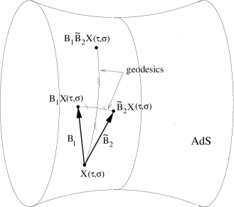
Figure 1: The superposition of two Bäcklund transformations. If we know $B_{\gamma_{1}}X(\tau,\sigma)$ and $\tilde{B}_{\gamma_{2}}X(\tau,\sigma)$ we can find $B_{\gamma_{1}}\tilde{B}_{\gamma_{2}}X(\tau,\sigma)$ by reflecting $X(\tau,\sigma)$ in the middle point of the geodesic interval connecting $B_{\gamma_{1}}X(\tau,\sigma)$ and $\tilde{B}_{\gamma_{2}}X(\tau,\sigma)$. Here $\gamma_{1}\simeq-1$ and $\gamma_{2}\simeq 1$.

2.2.4 Properties of Bäcklund transformations.

We will now describe some properties of the Bäcklund transformations. It follows from the Bäcklund equations (4) that the scalar product of $X(\tau,\sigma)$ and $B_{\gamma}X(\tau,\sigma)$ is a constant:

$$(X(\tau,\sigma),B_{\gamma}X(\tau,\sigma))={1-\gamma^{2}\over 1+\gamma^{2}}$$ (12)

This follows from considering the scalar product of Eqs. (4) with $B_{\gamma}X$ and $X$. Taking the scalar product of (4) with $\partial_{+}X$ and $\partial_{-}X$ and taking into account (12), we can see that the Bäcklund transformations preserve $|\partial_{+}X|$ and $|\partial_{-}X|$:

$$|\partial_{\pm}B_{\gamma}X|=|\partial_{\pm}X|$$ (13)

An important property (which in our definition follows from (2) and (3)) is the Permutability Theorem:

$$B_{\gamma_{1}}B_{\gamma_{2}}=B_{\gamma_{2}}B_{\gamma_{1}}$$ (14)

This theorem was proven in great generality in [35]. An immediate consequence of the commutativity and eqs. (4) is that $B_{\gamma_{1}}B_{\gamma_{2}}X$ is a linear combination of $X$, $B_{\gamma_{1}}X$ and $B_{\gamma_{2}}X$. The coefficients of this linear combination can be found from (12):

$$B_{\gamma_{1}}B_{\gamma_{2}}X-X={(X,B_{\gamma_{2}}X)-(X,B_{\gamma_{1}}X)\over 1-(B_{\gamma_{1}}X,B_{\gamma_{2}}X)}(B_{\gamma_{1}}X-B_{\gamma_{2}}X)$$ (15)

This is the “tangent rule” of Bäcklund transformations. For the target space ${\bf R}\times S^{2}$ the classical string is essentially equivalent to the sine-Gordon model, and the tangent rule (15) is closely related to the bilinear identity for the sine-Gordon $\tau$-function (see [25] and references there).

For $\gamma=\tilde{\gamma}$ our definition implies an interesting formula:

$$B_{\gamma}X=-\tilde{B}_{\gamma}X$$ (16)

This formula provides relations between the flows of the “left” local charges $\xi_{{\cal F}_{2n}}$ and the “right” local charges $\xi_{\widetilde{\cal F}_{2n}}$. We will use these relations in Section 2.3.2. Eq. (16) requires an explanation. Let us construct the “perturbative” solution $B_{\gamma}X$ of (4) using the null-surface perturbation theory. Because of the symmetry $X\leftrightarrow B_{\gamma}X$ of (4) there are two such solutions; we will choose the one which satisfies (6) when $\gamma$ is small (the other one should be denoted $B_{-\gamma}X$). One can see that $-B_{\gamma}X$ satisfies Eq. (5) for $\tilde{\gamma}=\gamma$. Therefore $-B_{\gamma}X$ is either $\tilde{B}_{\gamma}X$ or $\tilde{B}_{-\gamma}X$, and to verify the sign we have to verify Eq. (7). It is enough to verify Eq. (7) for the null-surface, that is when $\partial_{+}X=\partial_{-}X$. If we consider the null-surface, the solution of the Bäcklund transformation can be written down explicitly, see Eqs. (8) and (9). We see that indeed $B_{\gamma}X=-\tilde{B}_{\gamma}X$. But we must stress that (16) is, by our arguments, valid only in the sector of fast moving strings. We suspect that (16) might fail outside of the regime of the fast moving strings because of the possible problems with the definition of the canonical $B_{\gamma}$ (such as multivaluedness). In this paper we just consider the perturbation theory around the null-surface and use the perturbative definition of $B_{\gamma}$ from Section 2.2.2.

From (16) and (15) follows the tangent rule for $B_{\gamma_{1}}X$ and $\tilde{B}_{\gamma_{2}}X$:

$$B_{\gamma_{1}}\tilde{B}_{\gamma_{2}}X+X={(X,\tilde{B}_{\gamma_{2}}X)+(X,B_{\gamma_{1}}X)\over 1+(B_{\gamma_{1}}X,\tilde{B}_{\gamma_{2}}X)}(B_{\gamma_{1}}X+\tilde{B}_{\gamma_{2}}X)$$

This relation is illustrated on Fig. 1 where $\gamma_{1}\simeq-1$ and $\gamma_{2}\simeq 1$. Equations (4) and (5) are symmetric with respect to the exchange $X\leftrightarrow B_{\gamma}X$ and also under $\gamma\to-\gamma$ and therefore

$$B_{-\gamma}=B_{\gamma}^{-1}\;\;\;\mbox{and}\;\;\;\tilde{B}_{-\tilde{\gamma}}=\tilde{B}_{\tilde{\gamma}}^{-1}$$ (17)

2.2.5 Canonicity of Bäcklund transformations.

The way we defined Bäcklund transformations in Section 2.2.1, canonicity follows automatically from Eqs. (2), (3). But in fact it can be derived directly from the Bäcklund equations (4), (5). More precisely, if $B_{\gamma}X$ is defined as the periodic solution of (4), then the transformation $X\mapsto B_{\gamma}X$ is canonical. We will now prove it.

The symplectic form on the classical string phase space can be computed as the exterior derivative of the “symplectic potential” $\alpha$:

$$\omega=\delta\alpha$$ (18)

Here $\delta$ denotes the differential on the string phase space. We use $\delta$ instead of the usual notation $d$ for the differential to distinguish it from the $d$ acting on the differential forms on the string worldsheet. The symplectic potential is:

$$\alpha={1\over 2\pi}\int d\sigma(\delta X,\partial_{\tau}X)$$ (19)

The symplectic potential is a 1-form on the string phase space, because it contains one field variation $\delta X$. Therefore $\omega=\delta\alpha$ is a closed two-form on the string phase space. The integral in (19) is taken over the spacial contour on the worldsheet at some fixed $\tau=\tau_{0}$ and does depend on $\tau_{0}$. However its exterior derivative $\omega$ does not depend on $\tau_{0}$. More generally, we could consider a family of symplectic potentials depending on the closed contour $C$ on the worldsheet:

$$\alpha_{C}={1\over 2\pi}\oint_{C}(\delta X,*dX)$$ (20)

This expression does depend on the choice of the contour $C$, but its exterior derivative $\omega=\delta\alpha_{C}$ does not.

Eqs. (4) and (12) imply that the Bäcklund transformation changes the symplectic potential $\alpha$ by a $\delta$ of something:

$$B_{\gamma}^{*}\alpha-\alpha={1\over 2\pi}\int d\sigma(\delta B_{\gamma}X,\partial_{\tau}B_{\gamma}X)-{1\over 2\pi}\int d\sigma(\delta X,\partial_{\tau}X)=$$

$$=\delta\left(\;{1\over 2\pi}\int d\sigma(X,\partial_{\sigma}B_{\gamma}X)\right)$$ (21)

Therefore the symplectic form (18) does not change, which means that $B_{\gamma}$ is a canonical transformation.

2.2.6 The “logarithm” of the Bäcklund transformation.

Consider the Hamiltonian vector fields $\xi_{\gamma}$ and $\tilde{\xi}_{\tilde{\gamma}}$ defined as the “logarithms” of the left and right Bäcklund transformations:

$$\xi_{\gamma}=\sum_{n}t_{2n}({\gamma})\xi_{{\cal F}_{2n}},\;\;\;\tilde{\xi}_{\tilde{\gamma}}=\sum_{n}\sum_{n}\tilde{t}_{2n}(\tilde{\gamma})\xi_{\widetilde{\cal F}_{2n}}$$ (22)

If we define the Bäcklund transformations by Eqs. (4) and (5), then $\xi_{\gamma}$ and $\tilde{\xi}_{\tilde{\gamma}}$ can be defined, at least formally as power series in $\gamma$ and $\tilde{\gamma}^{-1}$, as follows. Let us first define $\xi_{\gamma}^{(1)}$:

$$\xi_{\gamma}^{(1)}=\gamma\left.{\partial\over\partial\gamma}\right|_{\gamma=0}B_{\gamma}X$$ (23)

This is a vector field on the phase space, which depends on $\gamma$ linearly. Now $e^{-\xi_{\gamma}^{(1)}}B_{\gamma}X=X+O(\gamma^{2})$ and therefore we can define $\xi_{\gamma}^{(2)}$:

$$\xi_{\gamma}^{(2)}=\xi_{\gamma}^{(1)}+{\gamma^{2}\over 2}\left.{\partial^{2}\over\partial\gamma^{2}}\right|_{\gamma=0}(e^{-\xi_{\gamma}^{(1)}}B_{\gamma}X)$$ (24)

We will have $e^{-\xi_{\gamma}^{(2)}}B_{\gamma}X=X+O(\gamma^{3})$. We can continue this process and define

$$\xi_{\gamma}^{(n+1)}=\xi_{\gamma}^{(n)}+{\gamma^{n+1}\over(n+1)!}\left.{\partial^{n+1}\over\partial\gamma^{n+1}}\right|_{\gamma=0}(e^{-\xi_{\gamma}^{(n)}}B_{\gamma}X)$$ (25)

The resulting formal series $\xi_{\gamma}=\xi_{\gamma}^{(\infty)}$ is a vector field on the phase space which could be thought of as a logarithm of $B_{\gamma}$:

$$B_{\gamma}=e^{\xi_{\gamma}}$$ (26)

The vector fields $\xi_{\gamma}$ and $\tilde{\xi}_{\tilde{\gamma}}$ are power series in $\gamma$ and $1/\tilde{\gamma}$. The coefficients of $\gamma$ and $1/\tilde{\gamma}$ are local vector fields on the string phase space. These vector fields are Hamiltonian, because the Bäcklund transformations are canonical. Therefore they are generated by some local conserved charges. We will describe the local conserved charges in Section 3 and explain how $\xi_{\gamma}$ and $\tilde{\xi}_{\tilde{\gamma}}$ are expressed through these local conserved charges.

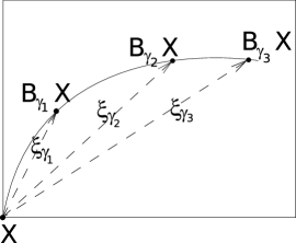
Figure 2: $B_{\gamma}$ and $\xi_{\gamma}$.

The relation between $B_{\gamma}$ and $\xi_{\gamma}$ is shown schematically on Fig.2. The solid curve represents the one-parameter family of solutions $B_{\gamma}X(\tau,\sigma)$ parametrized by the real $\gamma$. The dashed lines represent the trajectories of the Hamiltonian vector fields $\xi_{\gamma}$. For the finite-gap solutions, all $B_{\gamma}X$ belong to the same Liouville torus as $X$. The vectors $\xi_{\gamma}$ are the shifts on the torus corresponding to the Bäcklund transformations. But notice that our definition of the “logarithm” of the Bäcklund transformations did not require the knowledge of the fact that these transformations are generated by the flows of the local conserved charges. For us here, this fact is rather a consequence of the abstract definition of the logarithm. Generally speaking, the logarithmic map from the group of diffeomorphisms to the algebra of vector fields is notoriously ill-defined. But the Bäcklund transformation $B_{\gamma}$ is parametrized by a continuous parameter $\gamma$, and becomes the identical transformation at $\gamma=0$. This allows us to define $\xi_{\gamma}$ as a series in $\gamma$. In the null surface perturbation theory we have seen that $B_{\gamma}$ is at each order a rational function of $\gamma$ with the poles at $\gamma=\pm i$. This means that the series in $\gamma$ converge at least up to $\gamma=1$.

2.3 Deck transformation and Bäcklund transformations.

2.3.1 Deck transformation.

$AdS_{5}$ is the universal covering space of the hyperboloid $AdS_{5}/{\bf Z}$. In other words, the point $\hat{x}\in AdS_{5}$ can be thought of as a point of the hyperboloid $x\in AdS_{5}/{\bf Z}$, together with the path connecting $x$ to the fixed “base point” $x_{*}$. The path is considered modulo the homotopic equivalence (that is, two pathes are considered equivalent if one can be continuously deformed to the other).

The deck transformation is defined as the isometry of $AdS_{5}$ which does not change $x$, but changes the path from $x_{*}$ to $x$ by attaching to it a loop going once around the noncontractible cycle of the hyperboloid. We will denote the deck transformation $c^{2}$.

The existence of the large isometry group of $AdS_{5}$ allows us to express $c^{2}$ as a flow by the finite time generated by a Killing vector field. Namely, if $T$ is the global time of $AdS_{5}$ then

$$c^{2}=e^{2\pi{\partial\over\partial T}}$$ (27)

We defined $c^{2}$ as an isometry of the AdS space. It can be also considered a symmetry of the string phase space. Symmetries of the string theory following from the symmetries of space-time are called geometrical symmetries.

Figure 3: The deck transformation measures the deviation of the string worldsheet from being periodic in the global time. It is the “monodromy by the time $2\pi$”. The spiral represents the projection of the string worldsheet to the hyperboloid $AdS_{5}/{\bf Z}$. To simplify the picture we have imagined that the string is collapsed to a point. The noncontractible cycle of the hyperboloid corresponds to the time direction in AdS.

Eq. (27) tells us that $c^{2}$ is what corresponds in the classical string theory to the notion of the anomalous dimension in the dual Yang-Mills theory. Additional details can be found in [21].

The isometry group of $AdS_{5}$ is $\widetilde{SO}(2,4)$ — the universal covering of the orthogonal group. Notice that $\partial\over\partial T$ does not commute with the elements of $\widetilde{SO}(2,4)$ (in fact, it is one of the generators of the algebra $so(2,4)$). But $e^{2\pi{\partial\over\partial T}}$ does commute with $\widetilde{SO}(2,4)$; it is an element of the center of $\widetilde{SO}(2,4)$. Therefore Eq. (27) tells us that for the AdS space, the deck transformation can be understood as an element of the center of the symmetry group $\widetilde{SO}(2,4)$.

We can also interpret Eq. (27) as defining the “logarithm” of the deck transformation:

$$"{\partial\over\partial T}={1\over 2\pi}\log c^{2}\;"$$

But the logarithm is by no means an unambiguously defined operation. There are other vector fields exponentiating to $c^{2}$. In fact, when we consider the action of $c^{2}$ on the classical string phase space, there is a better choice for $\log c^{2}$ then $2\pi{\partial\over\partial T}$. It is better already because this $\log c^{2}$ (unlike ${1\over 2\pi}{\partial\over\partial T}$) commutes with $\widetilde{SO}(2,4)$; some additional motivation can be found in [21]. This alternative definition of $\log c^{2}$ relies on the existence of infinitely many local conserved charges ${\cal F}_{2k}$. Remember that we denote $\xi_{{\cal F}_{2k}}$ the corresponding Hamiltonian vector fields. It turns out that:

$$c^{2}=e^{\sum c_{k}\xi_{{\cal F}_{2k}}}$$ (28)

for some coefficients $c_{k}$. This does not mean that ${\partial\over\partial T}=\sum c_{k}\xi_{{\cal F}_{2k}}$, but only that the trajectories of the vector field ${\partial\over\partial T}-\sum c_{k}\xi_{{\cal F}_{2k}}$ are periodic with the period $1$. We have conjectured the formula of the type (28) in [21], based on the arguments of [34]. We will now give a proof based on the properties of Bäcklund transformations.

2.3.2 Deck transformation is a Bäcklund transformation.

Notice that equations (4) and (5) involve only the projection of the string worldsheet to the hyperboloid $AdS_{5}/{\bf Z}$. The string actually lives in $AdS_{5}$ which is the universal covering space of this hyperboloid. We can lift the action of the Bäcklund transformation from the string on the hyperboloid to the string on $AdS_{5}$ using the vector fields $\xi_{\gamma}$ and $\tilde{\xi}_{\tilde{\gamma}}$.

Let us define the continuous families of transformations $B_{\gamma}[s]=e^{s\;\xi_{\gamma}}$ and $\tilde{B}_{\tilde{\gamma}}[s]=e^{s\;\tilde{\xi}_{\tilde{\gamma}}}$ parametrized by a real parameter $s\in[0,1]$. We do not know if the transformations $B_{\gamma}[s]$ and $\tilde{B}_{\tilde{\gamma}}[s]$ have any special properties for an arbitrary $s$, but for $s=1$ we get the Bäcklund transformations. Now we have a pair of continuous families of solutions $B_{\gamma}[s]X$ and $\tilde{B}_{\tilde{\gamma}}[s]X$ connecting $B_{\gamma}X$ and $\tilde{B}_{\tilde{\gamma}}X$ to $X$. But the phase space of the classical string on $AdS$ is a cover of the phase space of the classical string on the hyperboloid, therefore the existence of a continuous family of transformations connecting the Bäcklund transformation to the identical transformation allows us to lift it from the string on the hyperboloid to the string on $AdS_{5}$.

Now consider the special case when $\gamma=\tilde{\gamma}$. Eq. (16) implies that for the fast moving strings:

$$\exp[2(\xi_{\gamma}-\tilde{\xi}_{\gamma})]=c^{2}$$ (29)

Indeed, Eq. (16) shows that the transformation $e^{2(\xi_{\gamma}-\tilde{\xi}_{\gamma})}$ acts on the string on the hyperboloid as the identical transformation. Therefore it acts on the string in $AdS$ either as the identical transformation or as some iteration of the deck transformation. We will argue that this is actually the deck transformation itself. We know that $e^{2(\xi_{\gamma}-\tilde{\xi}_{\gamma})}=\mbox{(deck)}^{k}$ where $k$ is some integer. Because of the continuity this integer cannot change when we continuously change the worldsheet. Therefore it is enough to find it for some particular worldsheet. Let us find $k$ in the limiting case when the fast moving string becomes a null-surface. In this case the Bäcklund transformations are given by (8) and (9):

$$B_{\gamma}X={1-\gamma^{2}\over 1+\gamma^{2}}X-{2\gamma\over 1+\gamma^{2}}{\partial_{\tau}X\over|\partial_{\tau}X|}$$ (30)

$$\tilde{B}_{\tilde{\gamma}}X={1-\tilde{\gamma}^{-2}\over 1+\tilde{\gamma}^{-2}}X+{2\tilde{\gamma}^{-1}\over 1+\tilde{\gamma}^{-2}}{\partial_{\tau}X\over|\partial_{\tau}X|}$$ (31)

This means that for the null-surface we have:

$$\xi_{\gamma}=-2{\arctan\gamma\over|\partial_{\tau}X|}{\partial\over\partial\tau}$$ (32)

$$\tilde{\xi}_{\tilde{\gamma}}=2{\arctan(1/\tilde{\gamma})\over|\partial_{\tau}X|}{\partial\over\partial\tau}$$ (33)

For $\gamma=\tilde{\gamma}$:

$$\xi_{\gamma}-\tilde{\xi}_{\gamma}=-\pi{1\over|\partial_{\tau}X|}{\partial\over\partial\tau}$$ (34)

In the null-surface limit each point of the string moves on the equator of $AdS_{5}$, and $e^{s(\xi_{\gamma}-\tilde{\xi}_{\gamma})}$ shifts by the angle $\pi s$ along the equator. Therefore for $s=2$ we go once around the noncontractible cycle of the hyperboloid; this is the deck transformation.

Let us summarize the relation between the Bäcklund transformations and the deck transformation. There are two continuous families of commuting canonical transformations $B_{\gamma}$ and $\tilde{B}_{\tilde{\gamma}}$. We defined them as power series in $\gamma$ and $\tilde{\gamma}^{-1}$, so $\gamma$ should be small and $\tilde{\gamma}$ should be large. But in the fast moving sector $B_{\gamma}$ and $\tilde{B}_{\tilde{\gamma}}$ can be analytically continued to finite values of $\gamma$ and $\tilde{\gamma}$. To get the deck transformation, we have to consider $\gamma=\tilde{\gamma}$:

$$c^{2}=B_{\gamma}^{2}\tilde{B}_{\gamma}^{-2}$$ (35)

This suggests that if $Q_{\gamma}$ and $\tilde{Q}_{\tilde{\gamma}}$ are the quantum operators corresponding to the Bäcklund transformations in the quantum theory, then the anomalous dimension on the field theory side [21] is:

$$e^{2\pi i\Delta E}=Q_{\gamma}^{2}\tilde{Q}_{\gamma}^{-2}$$ (36)

for any parameter $\gamma$. In this formula it is assumed that $Q_{\gamma}$ is defined first for small $\gamma$, and $\tilde{Q}_{\tilde{\gamma}}$ for large $\tilde{\gamma}$, and then analytically continued to the finite value $\gamma=\tilde{\gamma}\simeq 1$.

We have argued that $B_{\gamma}$ is an exponential of the infinite linear combination of the local charges. Therefore (35) implies (28).

3 Local Pohlmeyer charges.

3.1 The definition of Pohlmeyer charges.

The Pohlmeyer charges are the local conserved charges of the sigma-model. There are two series of these charges, which we call “left charges” ${\cal F}_{2k}$ and “right charges” $\tilde{\cal F}_{2k}$. They can be obtained from the Bäcklund transformation. The generating function of the Pohlmeyer charges is:

$${\cal F}_{left}(\gamma)={1\over 2\pi}\int d\sigma\left[\gamma(B_{\gamma}X,\partial_{+}X)+\gamma^{3}(B_{\gamma}X,\partial_{-}X)\right]$$ (37)

$${\cal F}_{right}(\tilde{\gamma})={1\over 2\pi}\int d\sigma\left[{1\over\tilde{\gamma}}(\tilde{B}_{\tilde{\gamma}}X,\partial_{-}X)+{1\over\tilde{\gamma}^{3}}(\tilde{B}_{\tilde{\gamma}}X,\partial_{+}X)\right]$$ (38)

Here $B_{\gamma}X$ and $\tilde{B}_{\tilde{\gamma}}X$ are defined as perturbative solutions of Eqs. (4), (5), (6), (7). The analogous formulas can be written for the Pohlmeyer charges of the $S^{5}$ part of the sigma-model.

The generating functions ${\cal F}_{left}(\gamma)$ and ${\cal F}_{right}(\tilde{\gamma})$ have an expansion in the even powers of $\gamma$ and $\tilde{\gamma}^{-1}$ respectively. The coefficients are the local conserved charges ${\cal F}_{2k},\tilde{\cal F}_{2k}$. But we can also solve the Bäcklund equations in the null-surface perturbation theory, using $1\over|\partial_{\tau}X|$ as a small parameter. When we solve the Bäcklund equations in the null-surface perturbation theory, each order of the expansion of $B_{\gamma}X$ in $1\over|\partial_{\tau}X|$ depends on $\gamma$ as a rational function. This means that at each order of the null-surface perturbation theory ${\cal F}_{left}(\gamma)$ and ${\cal F}_{right}(\tilde{\gamma})$ are rational functions of $\gamma$ and $\tilde{\gamma}$ respectively. Therefore in the null-surface perturbation theory ${\cal F}_{left}(\gamma)$ and ${\cal F}_{right}(\tilde{\gamma})$ have a well-defined analytic continuation to finite values of $\gamma$ and $\tilde{\gamma}$.

It was conjectured in [15] that there exist the “improved” charges ${\cal G}_{2k}^{left},{\cal G}_{2k}^{right}$ which are finite linear combinations of ${\cal F}_{2k}$ and $\tilde{\cal F}_{2k}$:

$${\cal G}_{2k}^{left}=\sum_{n=1}^{k}c_{k,n}{\cal F}_{2k}$$ (39)

with the property that in the null-surface perturbation theory

$${\cal G}_{2k}^{left}\simeq|\partial_{\tau}X|^{-k+1}\;\;\;(k\geq 2)$$ (40)

The null-surface expansion of the generating functions (37) and (38) is the expansion in the “improved” charges ${\cal G}^{left}_{2k}$. The coefficients of ${\cal G}^{left}_{2k}$ in the expansion of ${\cal F}_{left}(\gamma)$ are rational functions of $\gamma$. (Indeed, if we solve the Bäcklund equations in the null-surface perturbation theory, each order will depend on $\gamma$ as a rational function.) We will derive the explicit formula (52) using the plane wave limit (but our derivation of (52) works only under the assumption that the improved charges satisfying (40) exist).

We will now explain how the vector field $\xi_{\gamma}$ can be represented as the linear combination of the Hamiltonian vector fields generated by ${\cal F}_{2k}$ and $\widetilde{\cal F}_{2k}$. We already know that $\xi_{\gamma}$ is represented by a linear combination of the Hamiltonian vector fields generated by the local conserved charges, see Section 2.2.6. We will argue in Section 3.3.3 that there are no local conserved charges other than Pohlmeyer’s. Therefore $\xi_{\gamma}$ is a linear combination of the Pohlmeyer charges. We will fix the coefficients of this linear combination in Section 3.3.5.

3.2 The null-surface limit of $\xi_{\gamma}$.

In the null surface limit we have $|\partial_{\tau}X|>>|\partial_{\sigma}X|$ and therefore we can replace in Eq. (37) $\partial_{\pm}X\simeq{1\over 2}\partial_{\tau}X$. We get:

$${\cal F}_{left}(\gamma)\simeq{1\over 4\pi}\int d\sigma\gamma(1+\gamma^{2})(B_{\gamma}X,\partial_{\tau}X)\simeq-{\gamma^{2}\over 2\pi}\int d\sigma|\partial_{\tau}X|$$ (41)

where we have also used (30). The symplectic structure of the classical string is:

$$\omega={1\over 2\pi}\int d\sigma(\delta\partial_{\tau}X,\delta X)$$ (42)

Therefore in the null-surface limit the functional ${\cal F}_{left}(\gamma)$ generates the following Hamiltonian vector field:

$$\xi_{{\cal F}_{left}(\gamma)}.X=-\gamma^{2}{1\over|\partial_{\tau}X|}\partial_{\tau}X$$ (43)

On the other hand (32) gives us the formula for $\xi_{\gamma}$ in the null-surface limit:

$$\xi_{\gamma}=-2{\arctan\gamma\over|\partial_{\tau}X|}{\partial\over\partial\tau}$$ (44)

The null-surface limit is too strict and does not provide us enough information about $\xi_{\gamma}$ to determine its expansion in $\xi_{{\cal F}_{2k}}$. We will see that the plane wave limit is good enough for this purpose. In Section 3.3.5 we will derive the formula relating $\xi_{\gamma}$ to $\xi_{{\cal F}(\gamma)}$:

$$\xi_{\gamma}=2\int_{0}^{\gamma}{d\gamma\over\gamma^{2}(1+\gamma^{2})}\xi_{{\cal F}_{left}(\gamma)}$$ (45)

As we have already discussed, $\xi_{{\cal F}_{left}(\gamma)}$ is at each order of the null-surface perturbation theory a rational function of $\gamma$. For example, the zeroth approximation given by (43) depends on $\gamma$ as $\gamma^{2}$. Because of the integral transform (45), $\xi_{\gamma}$ is not a rational function of $\gamma$. For example the zeroth order (44) contains $\arctan\gamma$. But after the exponentiation $B_{\gamma}=e^{\xi_{\gamma}}$ becomes again a rational function in the null-surface expansion, for example the zeroth order is given by (30):

$$B_{\gamma}X={1-\gamma^{2}\over 1+\gamma^{2}}X-{2\gamma\over 1+\gamma^{2}}{\partial_{\tau}X\over|\partial_{\tau}X|}$$

3.3 The plane wave limit.

In the plane wave limit [28] the classical string becomes essentially the theory of free massive field. The Pohlmeyer charges in this limit can be written explicitly. It turns out that all the local conserved charges of the free massive field invariant under the global symmetry appear as the limits of the Pohlmeyer charges. Also, the Pohlmeyer charges remain linearly independent in the plane wave limit. This implies that all the local charges appearing in the expansion of $\xi_{\gamma}$ are Pohlmeyer charges, and allows to find the coefficients of the expansion. This gives Eq. (64). We then give a direct derivation of (64) without using the plane wave limit.

3.3.1 Pohlmeyer charges in the plane wave limit.

In the plane wave limit the motion of the string is restricted to the small neighborhood of the null-geodesic. The transverse components of $X$ become free fields $x^{I}$, $I=1,2,3,4$. We have $X^{1,2,3,4}=\epsilon x^{1,2,3,4}+o(\epsilon)$, where $\epsilon$ is a small parameter measuring the accuracy of the plane wave approximation. The longitudinal components are:

$$x_{+}=M(\tau-\tau_{0})-{\epsilon^{2}\over 2}x_{-}$$ (46)

$$\partial_{\tau}x_{-}=-{1\over 2M}\sum_{i=1}^{4}\left[(\partial_{\tau}x_{i})^{2}+(\partial_{\sigma}x_{i})^{2}-M^{2}x_{i}^{2}\right]$$ (47)

$$\partial_{\sigma}x_{-}=-{1\over M}\sum_{i=1}^{4}(\partial_{\tau}x_{i},\partial_{\sigma}x_{i})$$ (48)

Here $M=\epsilon^{2}J+\ldots$ where $J$ is the angular momentum, see the review section of [27] for details. The free equations of motion for $x^{I}$ are $(\partial_{\tau}^{2}-\partial_{\sigma}^{2}+M^{2})x^{I}=0$.

Let $\alpha^{I}_{n}$ be the Fourier modes of $x^{I}$. The generating function of the local conserved charges in the plane wave limit was computed in [27]:

$${\cal F}_{left}(\gamma)=-\gamma^{2}\left[E+(1+\gamma^{2})\sum\limits_{n=-\infty}^{\infty}\sum\limits_{I=1}^{4}{M(\omega_{n}+n)\over M^{2}+\gamma^{2}(\omega_{n}+n)^{2}}\alpha^{I}_{n}\overline{\alpha^{I}_{n}}\right]=$$

$$=-\tan^{2}\alpha\left[E+\sum\limits_{n=-\infty}^{\infty}\sum\limits_{I=1}^{4}{M^{-1}(\omega_{n}+n)\over 1+\sin^{2}\alpha[M^{-2}(\omega_{n}+n)^{2}-1]}\alpha^{I}_{n}\overline{\alpha^{I}_{n}}\right]$$ (49)

Here $E$ is the energy (corresponding to $\partial\over\partial T$), $\omega_{n}=\sqrt{M^{2}+n^{2}}$ and $\alpha$ is defined as follows:

$$\gamma=\tan\alpha$$ (50)

3.3.2 Improved charges.

The oscillator expansion of ${\cal G}^{left}_{2k}$ is

$${\cal G}^{left}_{2k}=\delta_{k,1}E+\sum\limits_{n=-\infty}^{\infty}\sum\limits_{I=1}^{4}{\omega_{n}+n\over M}\left[{(\omega_{n}+n)^{2}\over M^{2}}-1\right]^{k-1}\alpha^{I}_{n}\overline{\alpha^{I}_{n}}$$ (51)

This means that the coefficients of the expansion of ${\cal F}^{left}(\gamma)$ are rational functions of $\gamma$:

$${\cal F}_{left}(\gamma)=\tan^{2}\alpha\sum\limits_{k=1}^{\infty}(-1)^{k}(\sin\alpha)^{2k}\;{\cal G}^{left}_{2k}=\sum\limits_{k=1}^{\infty}(-1)^{k}{\gamma^{2k+2}\over(1+\gamma^{2})^{k}}\;{\cal G}^{left}_{2k}$$ (52)

We derived this formula in the plane wave limit, but the following statement should be true for general fast moving strings:

The local charges ${\cal G}^{left}_{2k}$ related to the generating function ${\cal F}_{left}(\gamma)$ by Eq. (52) are improved in a sense of Eq. (40).

Indeed, if we assume the existence of the “improved” charges characterized by (40) then the coefficients of these charges in the expansion of ${\cal F}_{left}(\gamma)$ are fixed unambiguously by the plane wave limit.

3.3.3 There are no local conserved charges other than Pohlmeyer’s and the charges corresponding to the global symmetries.

Given a local conserved charge, we can consider its leading term in the plane wave limit. It will be of the form

$$\int d\sigma\;\epsilon^{q}M^{\left(1-\sum_{j=1}^{q}k_{j}\right)}\partial^{k_{1}}x^{i_{1}}\cdots\partial^{k_{q}}x^{i_{q}}$$ (53)

The power of $M$ is found from the worldsheet scaling invariance. But the local conserved currents of the free field theory are all quadratic in oscillators, and therefore the local charge should have $q=0$ or $q=2$. These are either Pohlmeyer charges or global conserved charges.

If a nonzero conserved charge has a leading expression in the plane wave limit of the order $\epsilon^{3}$ or higher, then it is necessarily a nonlocal charge. This is because all the local conserved charges of the free massive field are quadratic in the oscillators, and therefore such a conserved charge would be nonlocal already in the plane wave limit.

Therefore a local conserved charge is completely fixed by its plane wave limit, and also all the local conserved charges are Pohlmeyer charges.

3.3.4 Pohlmeyer charges and quasimomenta.

The Pohlmeyer charges can be also obtained from the spectral invariants of the monodromy matrix. The precise relation between the Pohlmeyer charges and the quasimomenta for the classical string on $S^{5}$ was derived in [26] using the approach of [35]:

$$\begin{array}[]{rl}{\cal F}_{left}(\gamma)=-{i\over 2\pi}{\gamma^{3}\over 1+\gamma^{2}}&\left[p_{1}\left({1-i\gamma\over 1+i\gamma}\right)+p_{2}\left({1-i\gamma\over 1+i\gamma}\right)+\right.\\[5.0pt] &\left.+p_{3}\left({1+i\gamma\over 1-i\gamma}\right)+p_{4}\left({1+i\gamma\over 1-i\gamma}\right)\right]=\\[5.0pt] ={1\over\pi}{\gamma^{3}\over 1+\gamma^{2}}&\mbox{Im}\left[p_{1}\left({1-i\gamma\over 1+i\gamma}\right)+p_{2}\left({1-i\gamma\over 1+i\gamma}\right)\right]\end{array}$$ (54)

The quasimomenta $p_{1},p_{2},p_{3},p_{4}$ are the logarithms of the eigenvalues of the monodromy matrix [5, 6, 7, 8, 9].

In Section 4.2 of [27] we conjectured the integral formula for the energy shift:

$$\Delta E=-{1\over\pi}\int_{-\infty}^{\infty}{d\gamma\over\gamma^{2}(1+\gamma^{2})}{\cal F}_{left}(\gamma)$$ (55)

Eq. (52) shows that this formula encodes the expansion of $\Delta E$ as an infinite linear combination of the improved currents ${\cal G}^{left}_{2k}$. Now let us substitute the result (54) of [26] and change the integration variable $\gamma\to y={1-i\gamma\over 1+i\gamma}$. We get:

$$\Delta E=-{i\over 16\pi^{2}}\int\limits_{|y|=1}d\left(y+{1\over y}\right)[p_{1}(y)+p_{2}(y)+p_{3}(\overline{y})+p_{4}(\overline{y})]$$ (56)

Since $|y|=1$ we can rewrite this integral in the following way:

$$\Delta E=-{i\over 16\pi^{2}}\int\limits_{|y|=1}d\left(y+{1\over y}\right)\sum\limits_{j=1}^{4}\varepsilon_{j}p_{j}(y)$$ (57)

where $\varepsilon_{1,2}=1$ and $\varepsilon_{3,4}=-1$. The contour of integration is the circle $|y|=1$. Similar formulas for the energy shift were obtained in [6, 7, 8]. The contour can be deformed, in particular it does not have to go through the points $y=\pm 1$. But if we want to deform the contour, we should make sure that it does not cross the singularities of ${\cal F}_{left}$ which for the fast moving strings are located near $y=0,\infty$ (see Section 2.2.2; in the null-surface expansion all the poles are at $\gamma=\pm i$).

We will now give a proof of Eq. (55).

3.3.5 Generator of Bäcklund transformations.

The action of Bäcklund transformations on the oscillators in the plane wave limit was derived in [27]:

$$B_{\gamma}\alpha_{n}={M-i\gamma(\omega_{n}+n)\over M+i\gamma(\omega_{n}+n)}\alpha_{n}$$ (58)

where $M$ is the mass parameter of the plane wave theory (which we denoted $\mu$ in [27]) and $\omega_{n}=\sqrt{M^{2}+n^{2}}$. The coordinates $x_{+}$ (which corresponds to the time in the light-cone gauge) and $x_{-}$ transform under the Bäcklund transformations as follows:

$$x_{+}\to x_{+}-\arctan\gamma,\;\;\;x_{-}\to x_{-}+{2\over\epsilon^{2}}\arctan\gamma$$

This means that

$$\xi_{\gamma}\alpha_{n}=\log\left[{M-i\gamma(\omega_{n}+n)\over M+i\gamma(\omega_{n}+n)}\right]\alpha_{n}$$ (59)

$$\xi_{\gamma}x_{+}=-\arctan\gamma$$ (60)

$$\xi_{\gamma}x_{-}={2\over\epsilon^{2}}\arctan\gamma$$ (61)

Therefore the Hamiltonian $H_{\gamma}$ of $\xi_{\gamma}$ is:

$$H_{\gamma}=-2\arctan(\gamma)E-i\sum_{n}\log\left[{M-i\gamma(\omega_{n}+n)\over M+i\gamma(\omega_{n}+n)}\right]\alpha_{n}\overline{\alpha_{n}}$$ (62)

where $E$ generates $-{1\over\epsilon^{2}}{\partial\over\partial x_{-}}+{1\over 2}{\partial\over\partial x_{+}}$. On the other hand the generating function of the Pohlmeyer charges was also computed in [27]:

$${\cal F}_{left}(\gamma)=-\gamma^{2}\left[E+(1+\gamma^{2})\sum_{n}{M(\omega_{n}+n)\over M^{2}+\gamma^{2}(\omega_{n}+n)^{2}}\alpha_{n}\overline{\alpha_{n}}\right]$$ (63)

We see that the Pohlmeyer charges ${\cal F}_{2n}$ (which are the coefficients of $\gamma^{2n}$ in the expansion of ${\cal F}_{left}(\gamma)$) are linearly independent in the plane wave limit. Therefore the comparison of (62) and (63) allows us to fix the coefficients in the expansion of $H_{\gamma}$ in ${\cal F}_{2n}$. The result can be written in the following compact form:

$${\partial H_{\gamma}\over\partial\gamma}={2\over\gamma^{2}(1+\gamma^{2})}{\cal F}_{left}(\gamma)$$ (64)

We call $H_{\gamma}$ the “generator” of Bäcklund transformations. Eq. (64) relates $H_{\gamma}$ to the generating function of Pohlmeyer charges. It is closely related to the spectrality of the Bäcklund transformations which is explained in [18]. We will give a direct derivation of this equation in the next subsection.

Eq. (64) implies that $H_{\gamma}$ can be represented as an integral over the open contour:

$$H_{\gamma}=2\int_{0}^{\gamma}{d\gamma\over\gamma^{2}(1+\gamma^{2})}{\cal F}_{left}(\gamma)=$$ (65)

$$={i\over 8\pi}\int^{y={1-i\gamma\over 1+i\gamma}}dy\left({1\over y^{2}}-1\right)[p_{1}(y)+p_{2}(y)+p_{3}(\overline{y})+p_{4}(\overline{y})]$$

Here the integration contour in the $y$-plane starts at $y=1$ and goes along the circle $|y|^{2}=1$ to the point $y={1-i\gamma\over 1+i\gamma}$. Since $|y|=1$ we have:

$$H_{\gamma}=-{i\over 16\pi}\int\limits_{y={1+i\gamma\over 1-i\gamma}}^{y={1-i\gamma\over 1+i\gamma}}d\left(y+{1\over y}\right)\sum\limits_{j=1}^{4}\varepsilon_{j}p_{j}(y)$$ (66)

Figure 4: The contours for $H_{\gamma}$ and $\tilde{H}_{\tilde{\gamma}}$.

The contour goes along the circle $|y|=1$ through the point $y=1$. We see that the Bäcklund transformations are generated by the same integral as the deck transformation, but the contour is open. The positions of the endpoints depend on the parameter $\gamma$ of the Bäcklund transformation. When $\gamma$ is small we can compute this integral by expanding $\sum\varepsilon_{j}p_{j}(y)$ around $y=1$; this again tells us that the Bäcklund transformations are generated by the local conserved charges.

In Section (2.2.2) we have seen that $B_{\gamma}X$ is a rational function of $\gamma$ in the null-surface perturbation theory, with the poles at $\gamma=\pm i$. The same is true about ${\cal F}_{left}(\gamma)$, because ${\cal F}_{left}(\gamma)$ is related to $B_{\gamma}X$ by Eq. (37). Therefore, if we consider ${\cal F}_{left}(\gamma)$ as an expansion in powers of $\gamma$ near $\gamma=0$, then at each order of the null-surface expansion the series in $\gamma$ will converge at least up to $\gamma=1$. Eq. (65) tells us that $H_{\gamma}$ as a power series in $\gamma$ also converges in the null-surface expansion. Therefore, although our arguments for $B_{\gamma}=e^{\xi_{\gamma}}$ were based on the expansion in powers of $\gamma$, in fact this relation between $B_{\gamma}$ and $\xi_{\gamma}$ should be true in the null-surface expansion in some finite region of the parameter $\gamma$.

The generator of the right Bäcklund transformation $\tilde{H}_{\tilde{\gamma}}$ is given by the same formula as (66) except for the contour goes through $y=-1$. When $\gamma=\tilde{\gamma}$ the difference $H_{\gamma}-\tilde{H}_{\gamma}$ is given by the integral over the closed contour. Notice that for the fast moving string $H_{\gamma}-\tilde{H}_{\gamma}$ does not depend on $\gamma$. This is because the conserved charge generating the deck transformation (or the action variable [34]) cannot be deformed. It is natural to denote $H_{\gamma}-\tilde{H}_{\gamma}=H_{\infty}$. Eq. (35) implies that $H_{\infty}=\pi\Delta E$. Therefore we derived (55).

The integral formula (66) involves a particular combination of the quasimomenta $p_{1},p_{2},p_{3},p_{4}$. If we integrate other combinations of the quasimomenta, we will get some other Hamiltonians, which will be non-local even in the null-surface limit. In the plane wave limit these other combinations should give the conservation laws of the qubic and higher order in the oscillators (the local Pohlmeyer charges are quadratic). It would be interesting to see if they have any geometrical meaning like Bäcklund transformations.

3.4 A direct derivation of (64).

Here we will derive Eq. (64) without the use of the plain wave limit. The main ingredients are the canonicity of Bäcklund transformations (21) and the permutability (14) which implies that the conserved charges are invariant under the Bäcklund transformations. We will use an interpretation of a canonical transformation $(p,q)\mapsto(\tilde{p},\tilde{q})$ as defining a Lagrangian submanifold in the direct product of two copies of the phase space with the symplectic form $dp\wedge dq-d\tilde{p}\wedge d\tilde{q}$. (This Lagrangian submanifold is the graph of the canonical transformation.)

Let us fix a contour on the string worldsheet at $\tau=0$. The phase space is parametrized by the contours $X(\sigma)$ and $\partial_{\tau}X(\sigma)$ at $\tau=0$. Since $B_{\gamma}$ is a canonical transformation, the graph of $B_{\gamma}$ is a Lagrangian submanifold in the direct product of two phase spaces. We will call it $L_{\gamma}$. By definition $L_{\gamma}$ consists of pairs $(x,B_{\gamma}x)$, where $x$ is a point of the string phase space ($x$ is a pair $X(\sigma),\partial_{\tau}X(\sigma)$). Let us consider two points in the phase space, $x^{(1)}$ and $x^{(2)}$, and their Bäcklund transforms $B_{\gamma}x^{(1)}$ and $B_{\gamma}x^{(2)}$.

Let us integrate the 1-form $B_{\gamma}^{*}\alpha-\alpha$ introduced in Section 2.2.5 over a contour in $L_{\gamma}$ connecting $(x^{(1)},B_{\gamma}x^{(1)})$ to $(x^{(2)},B_{\gamma}x^{(2)})$. The integral will not depend on the choice of the contour, because $L_{\gamma}$ is a Lagrangian manifold. Let us denote the integral $I$. Eq. (21) implies:

$$I=\left.-{1\over 2\pi}\int d\sigma(\partial_{\sigma}X,B_{\gamma}X)\right|_{1}^{2}$$ (67)

where $F|_{1}^{2}$ means $F(x^{(2)})-F(x^{(1)})$. Let us now consider an infinitesimal variation of $\gamma$. On the new Lagrangian manifold $L_{\gamma+\delta\gamma}$ consider two points $(x^{(1)},B_{\gamma+\delta\gamma}x^{(1)})$ and $(x^{(2)},B_{\gamma+\delta\gamma}x^{(2)})$, connect them by a contour lying in $L_{\gamma+\delta\gamma}$ and consider the new value of the integral $I$. Let us calculate the variation of $I$:

$${\partial I\over\partial\gamma}=\left.{1\over 2\pi}\int d\sigma\left(\partial_{\tau}B_{\gamma}X,\left.{\partial B_{\gamma}X\over\partial\gamma}\right|_{X,\partial_{\tau}X}\right)\right|_{1}^{2}+\int_{1}^{2}\iota_{\partial_{\gamma}\xi_{\gamma}}\omega=$$

$$=\left.-{1\over 2\pi}\int d\sigma\left(\partial_{\sigma}X,\left.{\partial B_{\gamma}X\over\partial\gamma}\right|_{X,\partial_{\tau}X}\right)\right|_{1}^{2}$$ (68)

We have used Eq. (67). The vertical bar indicates that we differentiate with respect to $\gamma$ with the constant $X$ and $\partial_{\tau}X$ (that is, only $B_{\gamma}X$ and $\partial_{\tau}B_{\gamma}X$ changes).

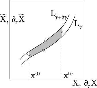
Figure 5: Because of the Stokes’ theorem the contour integral of the 1-form $\int d\sigma((\delta X,\partial_{\tau}X)-(\delta\widetilde{X},\partial_{\tau}\widetilde{X}))$ is equal to the integral over the strip of the 2-form $\int d\sigma((\delta X,\partial_{\tau}\delta X)-(\delta\widetilde{X},\partial_{\tau}\delta\widetilde{X}))$

The term $\int_{1}^{2}\iota_{\partial_{\gamma}\xi_{\gamma}}\omega$ on the left hand side appears when we integrate $\omega$ over the narrow strip between the path on $L_{\gamma}$ going from $(x^{(1)},B_{\gamma}x^{(1)})$ to $(x^{(2)},B_{\gamma}x^{(2)})$ and the path on $L_{\gamma+\delta\gamma}$ going from $(x^{(1)},B_{\gamma+\delta\gamma}x^{(1)})$ to $(x^{(2)},B_{\gamma+\delta\gamma}x^{(2)})$, see Fig. 5. It is equal to:

$$\int_{1}^{2}\iota_{\partial_{\gamma}\xi_{\gamma}}\omega=-{\partial H_{\gamma}\over\partial\gamma}(x^{(2)})+{\partial H_{\gamma}\over\partial\gamma}(x^{(1)})$$ (69)

Here we have used the permutability $B_{\gamma_{1}}B_{\gamma_{2}}=B_{\gamma_{2}}B_{\gamma_{1}}$ which implies that

$$H_{\gamma_{1}}(B_{\gamma_{2}}x)=H_{\gamma_{1}}(x)$$ (70)

In other words, the local conserved charges are preserved by the Bäcklund transformation. We have: $\partial_{\gamma}B_{\gamma}x=\partial_{\gamma}(e^{\xi_{\gamma}}.x)$. Because of the permutability this is equal to $(\partial_{\gamma_{1}}\xi_{\gamma_{1}}|_{\gamma_{1}=\gamma}).B_{\gamma}x$, in other words the value of the vector field $\partial_{\gamma}\xi_{\gamma}$ at the point $B_{\gamma}x$. And $\iota_{\partial_{\gamma}\xi_{\gamma}}\omega$ at the point $B_{\gamma}x$ is equal to $-d\partial_{\gamma}H_{\gamma}$ at the point $B_{\gamma}x$ (this is an element of the cotangent space to the phase space at the point $B_{\gamma}x$). Therefore the integral over the strip is equal to

$$-\left.{\partial\over\partial\gamma_{1}}\right|_{\gamma_{1}=\gamma}H_{\gamma_{1}}(B_{\gamma}x_{2})+\left.{\partial\over\partial\gamma_{1}}\right|_{\gamma_{1}=\gamma}H_{\gamma_{1}}(B_{\gamma}x_{1})$$

and because of (70) this is equal to the right hand side of (69). Combining Eqs. (69) and (68) we get:

$$\left.{\partial H_{\gamma}\over\partial\gamma}\right|_{X,\;\partial_{\tau}X}={1\over 2\pi}\int d\sigma\left[\left(\partial_{\sigma}X,\left.{\partial B_{\gamma}X\over\partial\gamma}\right|_{X,\;\partial_{\tau}X}\right)+\left(\partial_{\tau}B_{\gamma}X,\left.{\partial B_{\gamma}X\over\partial\gamma}\right|_{X,\;\partial_{\tau}X}\right)\right]$$

Now let us substitute $\partial_{\sigma}X+\partial_{\tau}B_{\gamma}X$ from the Bäcklund equation (4):

$$\partial_{\tau}B_{\gamma}X+\partial_{\sigma}X=-{1\over 2}(1+\gamma^{2})(B_{\gamma}X,\partial_{-}X)X-{1\over 2}(1+\gamma^{-2})(B_{\gamma}X,\partial_{+}X)X+\ldots$$ (71)

where dots denote terms proportional to $B_{\gamma}X$. Notice that $(X,\partial_{\gamma}B_{\gamma}X)=-{4\gamma\over(1+\gamma^{2})^{2}}$ because of (12). Therefore:

$$\left.{\partial H_{\gamma}\over\partial\gamma}\right|_{X,\;\partial_{\tau}X}={2\over 1+\gamma^{2}}{1\over 2\pi}\int d\sigma\left[\gamma(B_{\gamma}X,\partial_{-}X)+\gamma^{-1}(B_{\gamma}X,\partial_{+}X)\right]$$ (72)

This is (64), (37).

4 Conclusion.

We have discussed the deviation of the classical string worldsheet in AdS space from being periodic in the global time, which can be quantitatively characterized as the action of the deck transformation on the string phase space. This is important in AdS/CFT because it corresponds to the anomalous dimension on the field theory side. We have considered the deck transformation on the fast moving strings, in the null-surface perturbation theory. We have shown that at least in the null-surface perturbation theory the deck transformation can be understood as an example of the Bäcklund transformation (and in particular it can be connected to the identical transformation by a continuous family of Bäcklund transformations). This implies that the deck transformation can be understood as the finite time evolution by an infinite linear combination of the local conserved charges.

This can be easily understood in the plane wave limit, when the string worldsheet theory becomes a collection of the free massive fields. In this case, the energy is given by the formula:

$$E=J+\sum_{I=1}^{8}\sum_{n=-\infty}^{\infty}\overline{\alpha_{n}^{I}}\alpha_{n}^{I}+\sum_{k=0}^{\infty}c_{k}{\cal G}_{2k}$$

The first term on the right hand side is the $SO(2)$ angular momentum $J$ (integer), the second term is the total oscillator number (also integer), and the third term, which measures the deviation of $E$ from being integer, is an infinite sum of the local charges ${\cal G}_{k}$ with some coefficients $c_{k}$. On the field theory side the corresponding operator is of the form

$$\mbox{tr}\;\cdots ZZZ\;\Phi\;ZZZ\cdots ZZ\;\Phi\;ZZZZ\cdots$$

where $Z$ and $\Phi$ are complex scalars. From this point of view $J$ is the total number of the letters $Z$ under the trace, and $\sum_{I=1}^{8}\sum_{n=-\infty}^{\infty}\overline{\alpha_{n}^{I}}\alpha_{n}^{I}$ is the total number of the letters $\Phi$ (plus the total number of derivatives, if we include derivatives acting on $Z$ and $\Phi$). Therefore $\sum_{k=0}^{\infty}c_{k}{\cal G}_{2k}$ computes the anomalous dimension.

Having related the anomalous dimension to the Bäcklund transformations, we study the basic properties of the Bäcklund transformations and give an explicit formula (64) for the “generator” of the Bäcklund transformation. Eq. (64) is closely related to the general property of Bäcklund transformations which is called spectrality [18]. But in fact Eq. (64) is somewhat different from the usual definition of the spectrality. The definition of [18] used the generating function which requires the separation of the phase space variables into coordinates and momenta. We use instead the “generator” defined through the “logarithm” of the Bäcklund transformation.

The subject of Bäcklund transformations is one of the places where the classical theory of integrable systems touches the quantum theory. Therefore we hope that the considerations presented in this paper might be of some help in understanding the quantum worldsheet theory for the superstring in $AdS_{5}\times S^{5}$.

References

- [1] J. A. Minahan and K. Zarembo, “The Bethe-ansatz for N = 4 super Yang-Mills,” JHEP 03 (2003) 013, hep-th/0212208.
- [2] G. Mandal, N. V. Suryanarayana, and S. R. Wadia, “Aspects of semiclassical strings in AdS(5),” Phys. Lett. B543 (2002) 81–88, hep-th/0206103.
- [3] I. Bena, J. Polchinski, and R. Roiban, “Hidden symmetries of the AdS(5) x S**5 superstring,” Phys. Rev. D69 (2004) 046002, hep-th/0305116.
- [4] L. F. Alday, “Non-local charges on AdS(5) x S**5 and pp-waves,” JHEP 12 (2003) 033, hep-th/0310146.
- [5] V. A. Kazakov, A. Marshakov, J. A. Minahan, and K. Zarembo, “Classical / quantum integrability in AdS/CFT,” JHEP 05 (2004) 024, hep-th/0402207.
- [6] V. A. Kazakov and K. Zarembo, “Classical / quantum integrability in non-compact sector of AdS/CFT,” JHEP 10 (2004) 060, hep-th/0410105.
- [7] N. Beisert, V. A. Kazakov, and K. Sakai, “Algebraic curve for the SO(6) sector of AdS/CFT,” hep-th/0410253.
- [8] N. Beisert, V. A. Kazakov, K. Sakai, and K. Zarembo, “The algebraic curve of classical superstrings on AdS(5) x S**5,” hep-th/0502226.
- [9] S. Schafer-Nameki, “The algebraic curve of 1-loop planar N = 4 SYM,” Nucl. Phys. B714 (2005) 3–29, hep-th/0412254.
- [10] S. Frolov, A.A. Tseytlin, “Semiclassical quantization of rotating superstring in ”, JHEP 0206 (2002) 007, hep-th/0204226.
- [11] A.A. Tseytlin, “Semiclassical quantization of superstrings: and beyond”, Int. J. Mod. Phys. A18 (2003) 981, hep-th/0209116.
- [12] J.G. Russo, “Anomalous dimensions in gauge theories from rotating strings in ,” JHEP 0206 (2002) 038, hep-th/0205244.
- [13] S. Frolov, A.A. Tseytlin, “Multi-spin string solutions in x ,” Nucl.Phys. B668 (2003) 77-110, hep-th/0304255.
- [14] K. Pohlmeyer, “Integrable Hamiltonian systems and interactions through quadratic constraints,” Commun. Math. Phys. 46 (1976) 207–221.
- [15] G. Arutyunov and M. Staudacher, “Matching higher conserved charges for strings and spins,” JHEP 03 (2004) 004, hep-th/0310182.
- [16] S. Kharchev, A. Marshakov, A. Mironov, A. Morozov, and A. Zabrodin, “Towards unified theory of 2-d gravity,” Nucl. Phys. B380 (1992) 181–240, hep-th/9201013.
- [17] M. Gaudin and V. Pasquier, “The periodic Toda chain and a matrix generalization of the Bessel function’s recursion relations,” J. Phys. A25 (1992) 5243–5252.
- [18] E. K. Sklyanin, “Bäcklund transformations and Baxter’s Q-operator,” nlin.SI/0009009.
- [19] V. V. Bazhanov, S. L. Lukyanov, and A. B. Zamolodchikov, “Integrable Structure of Conformal Field Theory II. Q- operator and DDV equation,” Commun. Math. Phys. 190 (1997) 247–278, hep-th/9604044.
- [20] A. P. Veselov, “Growth and integrability in the dynamics of mappings,” Comm. Math. Phys. 145 (1992) 181–193.
- [21] A. Mikhailov, “Anomalous dimension and local charges,” hep-th/0411178.
- [22] L. Dolan, C. R. Nappi, and E. Witten, “A relation between approaches to integrability in superconformal Yang-Mills theory,” JHEP 10 (2003) 017, hep-th/0308089.
- [23] L. Dolan, C. R. Nappi, and E. Witten, “Yangian symmetry in D = 4 superconformal Yang-Mills theory,” hep-th/0401243.
- [24] L. Dolan and C. R. Nappi, “Spin models and superconformal Yang-Mills theory,” Nucl. Phys. B717 (2005) 361–386, hep-th/0411020.
- [25] A. Mikhailov, “An action variable of the sine-Gordon model,” hep-th/0504035.
- [26] G. Arutyunov and M. Zamaklar, “Linking Bäcklund and monodromy charges for strings on AdS(5) x S**5,” hep-th/0504144.
- [27] A. Mikhailov, “Plane wave limit of local conserved charges,” hep-th/0502097.
- [28] D. Berenstein, J. Maldacena and H. Nastase, ”Strings in Flat Space and PP-Waves from Super Yang-Mills”, JHEP 0204 (2002) 013, hep-th/0202021.
- [29] V. Kuznetsov and P. Vanhaecke, “Bäcklund transformations for finite-dimensional integrable systems: a geometric approach,” J.Geom.Phys. 44 (2002) 1–40, nlin.SI/0004003.
- [30] H. J. De Vega and A. Nicolaidis, “Strings in strong gravitational fields,” Phys. Lett. B295 (1992) 214–218.
- [31] H. J. de Vega, I. Giannakis, and A. Nicolaidis, “String quantization in curved space-times: Null string approach,” Mod. Phys. Lett. A10 (1995) 2479–2484, hep-th/9412081.
- [32] A. Mikhailov, “Speeding strings,” JHEP 12 (2003) 058, hep-th/0311019.
- [33] M. Kruczenski and A. A. Tseytlin, “Semiclassical relativistic strings in S**5 and long coherent operators in N = 4 SYM theory,” JHEP 09 (2004) 038, hep-th/0406189.
- [34] A. Mikhailov, “Notes on fast moving strings,” hep-th/0409040.
- [35] J. P. Harnad, Y. Saint-Aubin, and S. Shnider, “Bäcklund transformations for nonlinear sigma models with values in Riemannian symmetric spaces,” Commun. Math. Phys. 92 (1984) 329.