CERN–PH–TH/2005-136 IC/2005/042; LMU-ASC 55/05 hep-th/0507244
Open string topological amplitudes and gaugino masses

Abstract

We discuss the moduli-dependent couplings of the higher derivative F-terms $({\rm Tr}W^{2})^{h-1}$, where $W$ is the gauge $N=1$ chiral superfield. They are determined by the genus zero topological partition function $F^{(0,h)}$, on a world-sheet with $h$ boundaries. By string duality, these terms are also related to heterotic topological amplitudes studied in the past, with the topological twist applied only in the left-moving supersymmetric sector of the internal $N=(2,0)$ superconformal field theory. The holomorphic anomaly of these couplings relates them to terms of the form $\Pi^{n}({\rm Tr}W^{2})^{h-2}$, where $\Pi$’s represent chiral projections of non-holomorphic functions of chiral superfields. An important property of these couplings is that they violate R-symmetry for $h\geq 3$. As a result, once supersymmetry is broken by D-term expectation values, $({\rm Tr}W^{2})^{2}$ generates gaugino masses that can be hierarchically smaller than the scalar masses, behaving as $m_{1/2}\sim m_{0}^{4}$ in string units. Similarly, $\Pi{\rm Tr}W^{2}$ generates Dirac masses for non-chiral brane fermions, of the same order of magnitude. This mechanism can be used for instance to obtain fermion masses at the TeV scale for scalar masses as high as $m_{0}\sim{\cal O}(10^{13})$ GeV. We present explicit examples in toroidal string compactifications with intersecting D-branes.

1 Introduction

Possible relation between string theory and topological field theories may have profound origin and help in understanding the non-perturbative nature of the underlying fundamental theory. A concrete example is the topological partition function of the twisted Calabi-Yau sigma-model, $F^{(g,h)}$, defined on a general Riemann surface of genus $g$ having $h$ boundaries [1]. In the absence of holes, it is known that $F^{(g,0)}$ describes a sequence of higher derivative F-terms, ${\cal W}^{2g}$, in the effective four-dimensional (4d) $N=2$ supergravity, obtained upon compactification of Type II superstring on the corresponding Calabi-Yau manifold [2, 1]. Here, ${\cal W}$ is the chiral superfield of the $N=2$ gravity multiplet. Although $F^{(g,0)}$ is expected to be a holomorphic function of the chiral moduli, there is an anomaly which is captured by a set of recursion relations [1]. This non-holomorphicity is induced by an anomaly of the BRST current in the topological theory, while from the space-time point of view, it is due to the propagation of massless states that lead to non-localities in the effective action [2].

In this work, we perform a similar study of the genus-0 series $F^{(0,h)}$. In the presence of boundaries, $h\neq 0$, the topological twist involves D-branes, and thus supersymmetry is broken to $N=1$. The partition function $F^{(0,h)}$ describes a sequence of higher derivative F-terms, $({\rm Tr}W^{2})^{h-1}$, where $W$ is the chiral $N=1$ gauge superfield [1, 3, 4]. They give rise to amplitudes involving two gauge fields and $2(h-2)$ gauginos. In particular, we rederive the relation between the scattering amplitudes and the topological partition function by using the Neveu-Schwarz-Ramond formalism, similarly to Ref.[2]. The non-trivial property of this result is that in the physical amplitudes, besides the cancellation of the string oscillator contributions, there is a cancellation of the prefactor corresponding to the non-compact 4d momentum integration. This cancellation may not necessarily extend to higher genus amplitudes (involving additional insertions of closed string fields), although it certainly holds in the low energy effective field theory limit [3].

The same amplitudes have been computed in the past, in the context of Calabi-Yau compactifications of the heterotic string and were shown to be identical to the partition function of the topological theory obtained by twisting the left-moving supersymmetric sector which has $N=2$ superconformal symmetry [5]. However, unlike in the Type II case, the recursion relations describing the holomorphic anomaly of the heterotic topological partition function do not close among themselves. They involve a new class of topological quantities $F^{(0,h)}_{n}$, corresponding to correlation functions of anti-chiral fields, that describe F-terms of the type $\Pi^{n}({\rm Tr}W^{2})^{h-1}$, where $\Pi$’s are chiral projections of non-holomorphic functions of $N=1$ chiral superfields. Using Type I – heterotic string duality [6], one expects that the heterotic topological partition function at genus $h-1$ coincides with $F^{(0,h)}$ in the corresponding perturbative limit. On the Type I side, the non closure of the recursion relations among $F^{(0,h)}$’s is due to the existence of only one BRST charge on the boundaries, instead of two acting separately on left and right movers.

An important property of $F^{(0,h)}$ with $h\geq 3$ is the breaking of R-symmetry. A particularly interesting term is $({\rm Tr}W^{2})^{2}$. Combined with supersymmetry breaking induced by vacuum expectation values (VEV’s) of R-preserving D-term auxiliaries, it can generate Majorana gaugino masses, $m_{1/2}\sim\langle D\rangle^{2}\sim m_{0}^{4}$ (in string units), where $m_{0}$ is the scalar mass scale. In this work, we present an explicit calculation of $F^{(0,3)}$ on a world-sheet with three boundaries, in a simple example of Type IIB compactified on $T^{6}$ with magnetized D9 branes, or equivalently, upon T-duality, of intersecting D6 branes in Type IIA orientifolds [7]. In a vacuum configuration preserving $N=1$ supersymmetry, a non trivial $F^{(0,3)}$ is generated if one of the three brane stacks associated to the 3 boundaries is displaced away from the intersection of the other two; this implies the breaking of R-symmetry in the above example. On the other hand, if the brane configuration breaks supersymmetry, Majorana gaugino masses are generated. In the limit of small scalar masses, they behave as $m_{1/2}\sim m_{0}^{4}$ with a coefficient given precisely by the topological partition function $F^{(0,3)}$. Similarly, the $\Pi{\rm Tr}W^{2}$ term associated to the topological amplitude $F^{(0,2)}_{1}$ generates, upon supersymmetry breaking, one-loop masses for non-chiral brane fermions, of the same order as the gaugino masses.

Actually, the fact that a non-vanishing gaugino mass is generated at the perturbative order $(g=0,h=3)$, which corresponds to Euler characteristic $-1$, is in agreement with the general arguments of Ref.[8], based on $N=2$ superconformal $U(1)$ charge conservation. It is the same order as $(g=1,h=1)$, which corresponds to the gravitational mediation of supersymmetry breaking from the bulk to the gauge (brane) sector. This contribution depends strongly on the mechanism of supersymmetry breaking in the closed string sector [8], ignored in the present work. From the effective field theory point of view, the string diagram $(g=0,h=3)$ describes a particular gauge mediation by two-loop corrections in the gauge D-brane theory.
The paper is organized as follows.

$\bullet$ In Section 2, we describe the moduli space of the relevant world-sheet of genus zero with $h$ boundaries, $(g=0,h)$, as obtained by an appropriate involution of the Riemann surface of genus $g=h-1$ with no boundaries, $(g=h-1,0)$ [9, 10]. We also discuss the partition function and the so-called correction factors associated to Neumann and Dirichlet boundary conditions [10].

$\bullet$ In Section 3, we compute a string amplitude involving two gauge fields and $2(h-2)$ gauginos on a world-sheet of genus 0 with $h$ boundaries. We thus extract the coefficient of the F-term $({\rm Tr}W^{2})^{h-1}$ in the effective action, as a function of the closed string moduli parameterizing the Calabi-Yau geometry. For simplicity, we perform the computation for general $N=1$ intersecting brane configurations in $N=2$ orbifold compactifications of Type II superstrings. The generalization to Calabi-Yau is straightforward using the results of Ref.[2]. We show that this coupling-coefficient is given by the topological partition function $F^{(0,h)}$ of the associated twisted Calabi-Yau sigma-model.

$\bullet$ In Section 4, we discuss the holomorphic anomaly and the corresponding recursion relations. We first review the situation in the heterotic theory and then identify the possible contributions to the anomaly coming from various degeneration limits (dividing geodesic and handle) involving massless open and closed string states.

$\bullet$ In Section 5, we consider an explicit example of Type I string compactifications on a factorized $T^{6}=(T^{2})^{3}$ (instead of general orbifolds) with magnetized D9 branes, or equivalently with D6 branes at angles. We then compute $F^{(0,3)}$ in the case where the angles are chosen to preserve $N=1$ supersymmetry. We show that a non-zero answer is obtained if one of the three brane stacks associated to the three boundaries is moved away from the intersection of the other two, in each of the three tori. For non-parallel branes, this deformation does not change the spectrum, but breaks all R-symmetries. $F^{(0,3)}$ is expressed in a compact integral form as a function of $T^{6}$ moduli and Wilson lines.

$\bullet$ In Section 6, we compute the Majorana gaugino masses for arbitrary brane angles that break supersymmetry, originating from the same world-sheet with three boundaries. We show that in the $N=1$ supersymmetric limit, they behave as $m_{0}^{4}$, with $m_{0}$ the scalar mass, with a coefficient given by the topological partition function $F^{(0,3)}$, in accordance with the result of Section 5.

$\bullet$ In Section 7, we compute certain matter mass terms that are related to the F-terms appearing in the holomorphic anomaly of the gaugino mass $F^{(0,3)}$. These terms involve (twisted) charged fields from brane intersections.

$\bullet$ Section 8 contains some explicit examples. In particular, we consider the case of three stacks of branes forming pairwise three different $N=2$ supersymmetric sectors. We can then evaluate the $F^{(0,3)}$ integral explicitly, as well as all quantities related to it by the holomorphic anomaly, namely $F^{(0,2)}_{1}$ and $F^{(0,1)}_{2}$.

$\bullet$ Our results are summarized in Section 9 which also contains discussions on possible applications and open problems.

$\bullet$ Finally in the Appendix, we derive the lattice contribution of the twisted bosons to the topological partition functions $F^{(0,h)}$ for the case of magnetized D9 branes. This involves periods associated with Prym differentials and to our knowledge a detailed treatment of the zero modes associated with the twisted bosons for the open string case has not been made in the physics literature (for the closed string case see Ref.[11]). The result of this Appendix for the special case $h=3$ is used in sections 5 and 6.

2 Genus $g=0$ World-Sheet with $h$ Boundaries From the Involution of $g=h-1$ Riemann Surface

A planar ($h{-}1$)-loop open string world-sheet with $h$ boundaries, see Fig. 1,

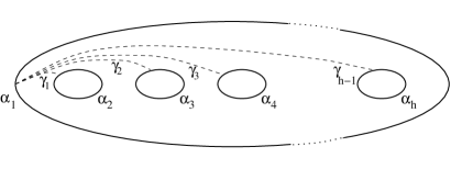
Figure 1: Open string world-sheet with $h$ boundaries.

admits a closed orientable genus $h{-}1$ double cover. The embedding is described by an anti-conformal involution, with the boundaries made of its fixed points. In the canonical homology basis, the a-cycles are invariant, ${\bf a}_{i}\to{\bf\bar{a}}_{i}={\bf a}_{i}$, while the b-cycles have their orientation reverted, ${\bf b}_{i}\to{\bf\bar{b}}_{i}={\bf b}_{i}^{-1}$, see Fig. 2.

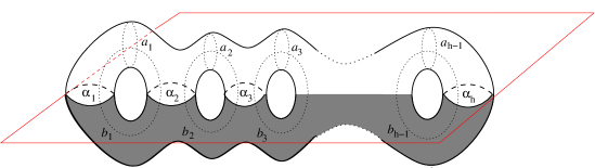
Figure 2: The involution (2.1) acts on the $g=h{-}1$ double-cover as a mirror reflection in the horizontal plane. The open string world-sheet is in the upper half while its mirror image is in the shaded lower half.

The anti-symplectic involution matrix has the form

$$I=\left(\begin{matrix}\ 1\!\!\!\!1&0\cr 0&-\ 1\!\!\!\!1\end{matrix}\right),$$ (2.1)

where $\ 1\!\!\!\!1$ is the $(h-1)\times(h-1)$ identity matrix. In terms of the a-cycles of the double cover, the boundaries of the $(g=0,h)$ world-sheet are ${\bf\alpha}_{1}={\bf a}_{1},\dots,\alpha_{k}={\bf a}_{k}\,{\bf a}_{k-1}^{-1},\dots,\alpha_{h}={\bf a}_{h-1}^{-1}$. It can be made into a contractible region by cutting along the curves $\gamma_{i}$, $i=1,\dots,h-1$, as shown in Fig. 1. The corresponding fundamental polygon is shown in Fig. 3.

Figure 3: The fundamental polygon obtained by cutting the open string world-sheet along the curves shown in Figure 1.

Under the involution, $\gamma_{i}\to\bar{\gamma}_{i}$, such that $\gamma_{i}\,\bar{\gamma}_{i}^{-1}={\scriptstyle\prod}_{k=1}^{k=i}{\bf b}_{k}$.

The period matrix $\tau$ of the double cover is restricted by the condition of invariance under the involution: ${\bar{\tau}}=I(\tau)=-\tau$, thus

$$\tau=it\,,$$ (2.2)

where $t$ is a real, symmetric matrix. Note that the positivity requirement for the period matrix now reads, in particular, $\det t>0$. The modular transformations that preserve the involution are represented by $Sp(2g,\mathbb{Z})$ matrices of the form

$$M=\left(\begin{matrix}(D^{-1})^{T}&0\cr 0&D\end{matrix}\right).$$ (2.3)

Since $D$ and $D^{-1}$ must be integer-valued, the “relative modular group” [10] is $GL(g,\mathbb{Z})$. This group essentially interchanges the boundaries, transforming the period matrix as $\tau\to D\tau D^{T}$. Note that since $\det D=\pm 1$, the determinant $\det t$ remains invariant.

The double cover endows the world-sheet with the basis of holomorphic differentials $\omega_{i}$ normalized as

$$\int_{{\bf a}_{j}}\omega_{i}=\delta_{ij}\quad,\quad\int_{{\bf b}_{j}}\omega_{i}=it_{ij},$$ (2.4)

The involution transforms them into anti-holomorphic differentials

$$\overline{\omega_{i}(z)}=\bar{\omega}_{i}(\bar{z})\quad;\quad\int_{\gamma_{j}}\omega_{i}-\bar{\omega}_{i}=i\sum_{k=1}^{k=j}t_{ik}.$$ (2.5)

Furthermore, the normalization condition (2.4) implies

$$\int_{{\alpha}_{m}}\omega_{n}=\delta_{mn}-\delta_{m(n-1)}\,.$$ (2.6)

For future use, we also need the surface integrals

$$\int\omega_{i}\wedge{\bar{\omega}}_{j}=\int d\left(\int^{z}\!\!\omega_{i}\right)({\bar{\omega}}_{j}-\omega_{j})$$ (2.7)

which, after using the fundamental polygon with the boundary conditions ${\bar{\omega}}_{j}|_{\alpha_{k}}=\omega_{j}|_{\alpha_{k}}$, become

$$\int\omega_{i}\wedge{\bar{\omega}}_{j}=\frac{i}{2}\sum_{k=1}^{k=h-1}\int_{\alpha_{k+1}}\!\!\!\omega_{i}\int_{\gamma_{k}}({\bar{\omega}}_{j}-\omega_{j})=\frac{t_{ij}}{2}.$$ (2.8)

In particular, the above result implies ${t_{ii}}>0$ for the diagonal elements of the period matrix.

The coordinates of a string propagating on a circle of radius $R$ have the form

$$X(P)=2\pi R\sum_{i=1}^{i=g}[L_{i}\int^{P}_{P_{0}}\omega_{i}(z)+\bar{L}_{i}\int^{P}_{P_{0}}\bar{\omega}_{i}(\bar{z})]\,,$$ (2.9)

where $P_{0}$ is an arbitrary base point. Due to the reality property ${\bar{\omega}}_{j}|_{\alpha_{k}}=\omega_{j}|_{\alpha_{k}}$, the Neumann (N) and Dirichlet (D) boundary conditions read, respectively,

$${\bar{L}}_{i}=\pm L_{i}\qquad\left\{{+~{}{\rm for}~{}N\atop-~{}{\rm for}~{}D}\right.$$ (2.10)

A string satisfying Neumann boundary conditions can wind around the boundaries $\alpha_{i}$. Keeping in mind the double cover, it is convenient to parameterize these windings in terms of the winding numbers $n_{i}$ around ${\bf a}_{i}$:

$$L_{i}^{N}=\frac{n_{i}}{2}\,.$$ (2.11)

On the other hand, in the Dirichlet directions, the boundary strings cannot wind, but an open string stretching between two different boundaries can wind from one end to the other. If it winds $m_{i}$ times between $\alpha_{i}$ and $\alpha_{i+1}$, then

$$L_{i}^{D}=i\sum_{j}(t^{-1})_{ij}m_{j}\,.$$ (2.12)

In terms of the double cover, $2m_{i}$ corresponds to the (even) number of windings around ${\bf b}_{i}$. The classical action, $S_{\rm cl}={1\over\pi\alpha^{\prime}}\int\partial_{z}X\partial_{\bar{z}}X$, can be computed by using (2.8):

$$S_{\rm cl}^{N}=\frac{\pi R^{2}}{2}\,nt\,n^{T}\qquad,\qquad S_{\rm cl}^{D}=2\pi R^{2}\,mt^{-1}m^{T}\,,$$ (2.13)

where $R$ is the compactification radius in $\alpha^{\prime}$ units.

The full partition function, in addition to the lattice sum $Z_{\rm cl}=e^{-S_{\rm cl}}$, includes the bosonic determinant factors. These can be obtained by taking the appropriate square root of the corresponding expression for the double cover:

$$(\det{\rm Im}\tau)^{-1/2}|Z_{1}|^{-1}\quad\longrightarrow\quad(R_{\Sigma}\det{\rm Im}\tau)^{-1/4}Z_{1}^{-1/2}\,,$$ (2.14)

where $Z_{1}$ is the chiral part of the determinant and $R_{\Sigma}$ is the “correction factor” depending on the boundary conditions [10]. For a general involution, it has the form

$$I=\left(\begin{matrix}\scriptstyle\Gamma&\scriptstyle 0\cr\scriptstyle\Delta&\scriptstyle\Gamma\end{matrix}\right)\,:\quad R_{\Sigma}^{\rm N}=(R_{\Sigma}^{\rm D})^{-1}=\det\left({1-\Gamma\over 2}{\rm Im}\tau+{1+\Gamma\over 2}({\rm Im}\tau)^{-1}\right).$$ (2.15)

Thus in our case,

$$R_{\Sigma}^{\rm N}=(\det t)^{-1}\qquad{\rm and}$$

$$(\det{\rm Im}\tau)^{-1/2}|Z_{1}|^{-1}\quad\longrightarrow\quad\left\{{Z_{1}^{-1/2}~{}\;\qquad\qquad~{}{\rm for}~{}N\atop(\det t)^{-1/2}Z_{1}^{-1/2}~{}{\rm for}~{}D}\right.$$ (2.16)

3 $W^{2(h-1)}$ F-terms from Open String Topological Amplitudes

In Type II theory, the F-terms of the form ${\cal W}^{2g}$, where $\cal W$ is the chiral $N=2$ supergravity multiplet, are determined at genus $g$ by the topological partition function $F_{g}$ [1, 2]. In this section, we discuss a similar structure in Type I theory: the open string diagrams with $h$ boundaries ($h{-}1$ open string loops) generate the effective action terms $({\rm Tr}\epsilon^{\alpha\beta}W_{\alpha}W_{\beta})^{(h-1)}$, where $W$ is the familiar chiral (spinorial) gauge field strength superfield and the trace is over gauge indices in the fundamental representation [1, 3, 4]. We will demonstrate this fact by evaluating the amplitudes involving $2(h{-}2)$ gauginos and two gauge bosons coupled to $h$ boundaries of a genus zero surface, in the Neveu-Schwarz-Ramond formalism, similarly to Ref.[2]. It is very convenient to describe this surface in terms of its $g=h{-}1$ double cover introduced in the previous section. Then the computation proceeds by essentially repeating the steps of the original computation in Type II theory.

We are interested in the effective action term $(\left.{\rm Tr}\epsilon_{\alpha\beta}W_{\alpha}W_{\beta})^{(h-1)}\right|_{\rm F}=(h{-}1){\rm Tr}[(\epsilon^{\alpha\beta}\lambda_{\alpha}\lambda_{\beta})^{(h-2)}g^{ac}g^{bd}{\cal F}_{ab}{\cal F}_{cd}]+\dots$, where $\lambda$ are gauginos and $\cal F$ are the self-dual combinations of gauge field strengths. Thus the amplitude under consideration involves $h{-}2$ pairs of gauginos at zero momentum, with opposite helicities inside each pair, plus one pair of gauge bosons in the momentum-helicity configuration corresponding to a self-dual gauge field strength. In order to provide the desired gauge charge, helicity and momentum configuration, the gaugino vertex operators are distributed in pairs among $h{-}2$ boundaries, the two gauge boson vertices are inserted on a separate boundary while one boundary remains “empty”.

The gaugino vertex operator of definite helicity $\alpha$, at zero momentum, in the canonical $-1/2$ ghost picture, reads:

$$V^{(-1/2)}_{\alpha}(x)=:e^{-\varphi/2}S_{\alpha}S_{int}:\,,$$ (3.1)

where $x$ is a position on the boundary of the world-sheet, $\varphi$ is the scalar bosonizing the superghost system, and $S_{\alpha}$ ($S_{int}$) is the space-time (internal) spin field. Upon complexification of the four space-time fermionic coordinates, $\psi_{I}$ for $I=1,2$, and introducing the bosonization scalars $e^{i\phi_{I}}=\psi_{I}$, one has

$$S_{\alpha}=e^{\pm\displaystyle{i\over 2}(\phi_{1}+\phi_{2})}\quad;\quad\alpha=\pm\,.$$ (3.2)

The gauge boson vertex operator at momentum $p$ and polarization $\epsilon$, in the $0$ ghost picture, is:

$$V_{p,\epsilon}^{(0)}(x)~{}=~{}:\!\epsilon_{\mu}(\partial X^{\mu}+ip\cdot\psi\psi^{\mu})e^{ip\cdot\!X}\!:~{}.$$ (3.3)

The above vertices must be supplemented by the appropriate Chan-Paton factors, which we omit here for simplicity.

In order to balance the ghost charge, we change one half of gaugino vertex operators to $+1/2$ ghost picture: this is done by inserting $h{-}2$ picture changing operators at the boundaries. Recall that the picture changing operator (PCO) is defined as $e^{\varphi}T_{F}$, where $T_{F}$ is the world-sheet supercurrent. In addition, due to the supermoduli integration, there are the usual $2g{-}2$ PCO insertions on the genus $g$ double cover that can be realized as $2(h{-}2)$ boundary insertions on the open string world-sheet. As a result, the total number of PCO insertions is $3(h{-}2)$.

We will see below that the purely bosonic parts of the gauge boson vertex operators do not contribute to the amplitude under consideration. To make the calculation simpler, we choose a kinematical configuration corresponding to $\psi_{1}\psi_{2}$ from one vertex and to $\bar{\psi}_{1}\bar{\psi}_{2}$ from the second. The amplitude then becomes

$$A_{h}=\langle\prod_{i=1}^{h-2}e^{-\varphi/2}S_{+}S_{int}(x_{i})\prod_{i=1}^{h-2}e^{-\varphi/2}S_{-}S_{int}(y_{i})\,\psi_{1}\psi_{2}(z){\bar{\psi}}_{1}{\bar{\psi}}_{2}(w)\!\!\prod_{i=1}^{3(h-2)}\!\!e^{\varphi}T_{F}(z_{i}){\rangle}_{h}$$ (3.4)

The above expression has exactly the same structure as the left-moving (or right-moving) part of the topological amplitude written in Eq.(3.6) of Ref.[2]. The amplitudes of Ref.[2] describe scattering processes involving graviphotons and gravitons; here, these particles are replaced by gauginos and gauge bosons, respectively. Now the vertex positions $x_{i}$, $y_{i}$, $z$ and $w$ are integrated over the boundary while the supercurrents are inserted at a priori arbitrary points $z_{i}$ of the boundary. In order to demonstrate a similar, topological nature of $A_{h}$, we can limit our considerations to the case of orbifold compactifications. The twists around b-cycles of the double cover correspond to the brane angles, while the twists around a-cycles belong to the orbifold group of the Type II theory. Thus, the former are fixed by the brane configuration, while the latter are summed over all elements of the orbifold group. Below, we call both types of periodicity conditions as orbifold twists.

In the case of orbifolds, the internal $N=2$ SCFT is realized in terms of free bosons and fermions. We consider for simplicity orbifolds realized in terms of $3$ complex bosons $X_{I}$ and left- (right-) moving fermions $\psi_{I}$ ($\widetilde{\psi}_{I}$), with $I=3,4,5$. Since all vertices involving these fermions are inserted at the boundary, from now on we can identify the left- and right-movers. Let $h_{O}$ be an orbifold twist defined by $h_{O}=\{h_{I}\}$, and its action on $X_{I}$ is $X_{I}\rightarrow e^{2\pi ih_{I}}X_{I}$ and similarly for $\psi_{I}$. Space-time supersymmetry implies that one can always choose the $h_{I}$’s to satisfy the condition:

$$\sum_{I}h_{I}~{}=~{}0\ .$$ (3.5)

On the genus $g=h{-}1$ double cover, we must associate one orbifold twist to each homology cycle ${\bf a}_{i},{\bf b}_{i}$, for $i=1,\cdots,h{-}1$. In the following we shall denote by $\{h_{O}\}=\{\{h_{I}\}\}$ the set of all twists along different cycles. One can bosonize the complex fermions

$$\psi_{I}=e^{i\phi_{I}}~{},~{}~{}~{}~{}~{}~{}~{}~{}~{}~{}~{}~{}~{}\bar{\psi}_{I}=e^{-i\phi_{I}}~{}.$$ (3.6)

In terms of these bosons, the internal part of gaugino vertex operators reads

$$S_{int}=e^{\displaystyle{i\over 2}(\phi_{3}+\phi_{4}+\phi_{5})}\,.$$ (3.7)

Similarly, the internal part of the supercurrent at the boundary becomes

$$T_{F}^{int}=G^{-}+G^{+}\quad;\quad G^{-}=\sum_{I=3}^{5}e^{-i\phi_{I}}\partial X^{I}\,.$$ (3.8)

By internal charge conservation, since all $2(h{-}2)$ gauginos carry charge $+1/2$ for $\phi_{3}$, $\phi_{4}$ and $\phi_{5}$, only the internal parts (3.8) of the supercurrents contribute: $h{-}2$ $T_{F}$’s must contribute $-1$ charge each for $\phi_{3}$ and similarly $-1$ for $\phi_{4}$ and $\phi_{5}$ each. Thus only $G^{-}$ contributes in this amplitude.

In order to compute the amplitude 3.4, we repeat the steps leading from Eq.(3.6) to Eq.(3.18) of Ref.[2]. In particular, in order to cast the contribution of world-sheet fermions into a form that makes the summation over their spin structures tractable by using the simplest form of Riemann identity for theta functions, we are led to the following choice of the supercurrent insertion points:

$$\sum_{a=1}^{3(h-2)}z_{a}~{}=~{}\sum_{i=1}^{h-2}y_{i}-z+w+2\Delta~{},$$ (3.9)

where $\Delta$ is the Riemann $\theta$ constant associated to the double cover. Note that this is an allowed gauge choice even if all points are located at the boundary. After summing over all spin structures and using exactly the same bosonization formulae and theta function identities as in section 3 of Ref.[2], we obtain the following expression

$$A_{h}~{} = \det{\omega_{i}(x_{j},z)}\det{\omega_{i}(y_{j},w)}\frac{\prod_{I}\det{(\partial X_{I}\omega_{-h_{I},i}(u_{j,I}))}}{\det h_{a}(z_{b})}$$ (3.10)

$$\epsilon_{a_{1},\cdots,a_{3(h-2)}}\prod_{i=1}^{3(h-2)}\int(\mu_{i}h_{a_{i}})\,({\makebox{lattice sum}})~{},$$

where $\partial X_{I}$ are the instanton modes twisted along the homology cycles by a particular set of orbifold twists $\{h_{I}\}$ and $\omega_{-h_{I},i}$, $i=1,\dots,h-2$, are the differentials associated to the boundary conditions twisted by $\{e^{-2i\pi h_{I}}\}$. The above expression is written for one particular partition $u_{i,I}~{}(i=1,\dots,h-2)$, $I=3,4,5$ of the positions of $T_{F}$’s which contribute $-1$ charge for $\phi_{3}$, $\phi_{4}$ and $\phi_{3}$, respectively. At the end, one must consider all possible partitions $\{u_{i,I}\}$ and antisymmetrize; note that as a set $\{z_{a}\}=\bigcup_{i,I}\{u_{i,I}\}$. Finally, $h_{a}$, $a=1,\dots,3(h-2)$ are the $3(h-2)$ quadratic differentials whose determinant appears after a number of technical steps explained in Ref.[2], making use of the bosonization formulae. They also appear as the zero modes of $b$-ghosts, contracted with the Beltrami differentials $\mu_{i}$; the corresponding integral gives the measure over moduli space of genus zero surfaces with $h$ disconnected boundaries.

There is only one difference between Eq.(3.10) and the analogous Eq. (3.18) of Ref.[2]: the absence of $(\det{\rm Im}\tau)^{-2}$ factor which arises in Type II theory after integrating over the space-time zero modes $X^{\mu}$ (i.e. the four-dimensional momenta). In our case, the correction factor (2.15) for the Neumann boundary condition eliminates this determinant, c.f. Eq.(2.16). Furthermore, for each compact direction, there is a lattice weight $Z_{cl}=e^{-S_{cl}}$, see Eq.(2.13), which according to Eq.(2.16) should be multiplied by $(\det t)^{-1/2}$ only in the case of Dirichlet boundary conditions.

The result (3.10) is for a fixed partition $\{u_{i,I}\}$ of the $z_{a}$’s. As mentioned earlier one must consider all possible partitions and antisymmetrize. Furthermore, $\partial X_{I}\omega_{-h_{I},i}$ are holomorphic quadratic differentials. Therefore, summing aver all partitions $\{u_{i,I}\}$ with the proper antisymmetrization gives:

$$\sum_{\{u\}}\prod_{I}\det(\partial X_{I}\omega_{-h_{I},i}(u_{i,I}))~{}=~{}B\det h_{a}(z_{b})~{},$$ (3.11)

where $B$ is $z_{a}$-independent. In this way, the amplitude (3.10) becomes manifestly independent of the PCO’s insertion points.

Now it remains to integrate the vertex positions $x_{i}$, $y_{i}$, $z$ and $w$ over all $h$ disconnected boundaries $\alpha$. For $z$ and $w$ located at a specific boundary $\alpha_{k}$, each pairing $(x,y)$ of opposite helicity gauginos at other boundaries gives rise to a specific Chan-Paton factor and, as a consequence of Eq.(2.6), it picks up only one of the $(h-1)!^{2}$ terms from the product $\det{\omega_{i}(x_{j},z)}\det{\omega_{i}(y_{j},w)}$. The integral of such a term is simply 1. As a result,

$$A_{h}~{}=~{}N\,h!\int_{{\cal M}_{h}}B\det{\int({\mu_{a}}h_{b}})\,({\rm{lattice~{}sum}})~{},$$ (3.12)

where ${{\cal M}_{h}}$ is the moduli space of genus 0 Riemann surfaces with $h$ boundaries. The combinatorial factor $h!$ arises as follows. First, there are $h$ choices of the “empty” boundary, then $h{-}1$ choices of the gauge bosons’ boundary and finally, $(h{-}2)!$ ways of distributing say positive helicity gauginos – the positions of negative helicity gauginos determines the Chan-Paton factor. The additional factor $N$ comes from the “empty” boundary and counts the number of D-branes.

The effective action term that reproduces the amplitude (3.12) is the F-term

$$S_{\rm eff}=\left.F^{(0,h)}({\rm Tr}\epsilon^{\alpha\beta}W_{\alpha}W_{\beta})^{(h-1)}\right|_{F},$$ (3.13)

with the coefficient given by the topological partition function

$$F^{(0,h)}~{}=~{}N\,h\int_{{\cal M}_{h}}\prod_{a=1}^{3h-6}{\int({\mu_{a}}G^{-}})\,({\rm{lattice~{}sum}})\,,$$ (3.14)

where we have used Eqs.(3.11) and (3.12). Here $G^{-}=\sum_{I}\partial X^{I}\bar{\psi}^{I}$ is the supercurrent in the topological twisted theory. Note that in the latter $\bar{\psi}^{I}$ carry dimension 1 and therefore they have $h-2$ zero modes $\omega_{-h_{I},i}$ with $i=1,...,h-2$.

4 Holomorphic Anomaly and $\Pi$-terms

Type I models considered above are dual to heterotic models. In particular the $N=1$ Type I models should be dual to heterotic models based on an $N=(2,0)$ world-sheet superconformal field theory. Correspondingly the topological amplitudes giving rise to F-terms $F^{(0,h)}({\rm Tr}W^{2})^{h-1}$ in Type I has a counterpart in heterotic theory. In Ref.[5], such amplitudes were shown to be given by partition functions of topological heterotic theory obtained by twisting the left-moving $N=2$ superconformal algebra. Indeed genus $g$ partition function of the topological heterotic theory $F^{H}_{g}$ gives the coupling $F^{H}_{g}({\rm Tr}W^{2})^{g}$.

The topological partition functions in Type II theories satisfy a holomorphic anomaly equation; their derivatives with respect to anti-holomorphic moduli can be expressed in terms of topological partition functions of lower genera. In the heterotic theory, however, as shown in Ref.[5], anti-holomorphic derivatives of $F^{H}_{g}$ give rise to a larger class of “topological” quantities $F^{H}_{g,n}$ labeled by genus $g$ and insertions of $n$ pairs of anti-chiral operators. In the effective field theory, these quantities are associated to F-terms of the form $({\rm Tr}W^{2})^{g}\Pi^{n}$. Let us briefly recall this difference between the Type II and heterotic topological theories.

The left-moving $N=2$ superconformal algebra is generated by the stress tensor $T$, a $U(1)$ current $J$ and the two dimension $3/2$ superconformal generators $G^{+}$ and $G^{-}$ where the superscripts $\pm$ refer to their $U(1)$ charges. Topological twisting of this algebra amounts to modifying $T\rightarrow T+\frac{1}{2}\partial J$. With respect to the new $T$ the dimensions of $G^{+}$ and $G^{-}$ are respectively $1$ and $2$. One defines the BRST operator for the topological theory $Q_{BRST}$ as the contour integral of $G^{+}$ current. $G^{-}$ having dimension $2$ and satisfying the condition $Q_{BRST}G^{-}=T$ plays the role of the $b$ ghost field of the string theory. Thus the measure on the moduli space of a Riemann surface of genus $g$ is defined by computing the correlation function of $3g-3$ $G^{-}$’s which are each folded with a Beltrami differential. The physical states of the theory are given by the $Q_{BRST}$-cohomology; the chiral primaries $\phi_{i}^{+}$ having charge $+1$ have now zero dimension, they are in $Q_{BRST}$-cohomology and can be inserted at punctures on the Riemann surfaces, while the anti-chiral vertex operators (in the 0 picture in string theory) are BRST exact operators $Q_{BRST}\phi_{\bar{i}}^{-}=\oint G^{+}\phi_{\bar{i}}^{-}$. Inserting such an operator in the Riemann surface gives a total holomorphic derivative in the world-sheet moduli $\partial_{t}$, since by deforming the contour $Q_{BRST}$ will act on one of the $G^{-}$ folded with the Beltrami differentials and convert it to $T$. Thus the only possible contributions can come from the boundaries of the moduli space of the world-sheet, namely the degenerations of the original Riemann surface along some non-trivial cycle which could be either homologically trivial or non-trivial.

In the homologically trivial degeneration limit, the surface splits into two Riemann surfaces $\Sigma_{1}$ and $\Sigma_{2}$ of lower genera, say genus $g_{1}$ and $g_{2}$, with one puncture each at $P_{1}$ and $P_{2}$. The operator $\phi_{\bar{i}}^{-}$ will be on one of the surfaces (say $\Sigma_{1}$). Since in the twisted theory the total charge on the sphere must be +3, it follows that the operators that appear at $P_{1}$ and $P_{2}$ are dual of each other and carry charges +2 and +1, respectively. The Beltrami differentials together with $G^{-}$ split on the two surfaces according to the $U(1)$ charge conditions in the twisted theory. The resulting term is of the form

$$F^{g_{1}}_{\bar{i},\bar{j}}G^{\bar{j}j}D_{j}F^{g_{2}}\,,$$ (4.1)

where $D$ is the holomorphic covariant derivative, and $j$ denotes the chiral operator carrying charge +1 at $P_{2}$, while the operator at $P_{1}$ carrying charge +2 is related to the anti-chiral operator (with charge $-1$) labeled by $\bar{j}$ by the action of a holomorphic 3-form operator $\rho(z)$ carrying charge +3:

$$\phi_{\bar{j}}^{-}\to\phi_{\bar{j}}^{++}\equiv\oint dz\rho(z)\phi_{\bar{j}}^{-}\,.$$ (4.2)

Such an operator $\rho$ of dimension 0 in the twisted theory exists for all $N=2$ superconformal field theories leading to space-time supersymmetry: $\rho=e^{i{\sqrt{3}}H}$ with ${\sqrt{3}}\partial H$ being the $U(1)$ current. The metric $G_{j\bar{j}}$ appearing in Eq.(4.1) is defined by the inner product $\langle\phi_{j}^{+}\phi_{\bar{j}}^{++}\rangle$. In Ref.[5], these new topological objects $F^{g}_{\bar{i},\bar{j}}$ were related to the couplings of the effective action terms $({\rm Tr}W^{2})^{g}\Pi$, denoted symbolically $F^{g}_{1}$. By further taking anti-holomorphic derivatives of these terms one arrives at generalized topological quantities denoted by $F^{g}_{\bar{i}_{1}...\bar{i}_{n};\bar{j}_{1}...\bar{j}_{n}}$ where $\bar{i}_{k}$ denote charge $-1$ insertions while $\bar{j}_{k}$ denote charge +2 insertions. These quantities were identified with the effective action terms $({\rm Tr}W^{2})^{g}(\Pi)^{n}$.

Similar reasoning for the case of handle degeneration results in a term of the form

$$C^{j\bar{j}}D_{j}F^{g-1}_{\bar{i},\bar{j}}$$ (4.3)

with

$$C^{j\bar{j}}=G^{j\bar{k}}Q_{\bar{k}\ell}G^{\ell\bar{\ell}}Q_{\bar{\ell}k}G^{k\bar{j}}\,,$$ (4.4)

where $Q$ is the charge operator associated with the gauge field $W$ (recall that in the heterotic theory the non-topological right moving part of the gauge vertex contains the charge operator). This is because only $2g-2$ of the original $2g$ gauge superfields sit on the genus $g-1$ surface obtained from the handle degeneration and the remaining two $W$’s sit at the node. As a result, the propagator connecting the two punctures $P_{1}$ and $P_{2}$ comes with the charges of the two $W$’s.

In Type II, we have also the right-moving $N=2$ superconformal algebra, which upon twisting gives rise to another BRST operator $\bar{Q}_{BRST}$. The anti-chiral vertex operators now (in the (0,0) ghost picture) are of the form $Q_{BRST}\bar{Q}_{BRST}\phi^{--}$ and inserting it gives rise to a double derivative $\partial_{t}\partial_{\bar{t}}$ in the moduli space integrals, where $t$ is standard plumbing fixture coordinate describing the degeneration of the surface. To get a non- vanishing contribution at $t\rightarrow 0$ the integrand must behave as $\ln(t\bar{t})$. The latter behavior is obtained only if the operator $\phi^{-}$ approaches the node (the puncture $P_{1}$) and has a non-vanishing structure constant $C_{\bar{i}\bar{j}\bar{k}}$ for some $\bar{k}$, the integral of its position giving rise to $\ln(t\bar{t})$. As a result

$$F^{g}_{\bar{i},\bar{j}}=e^{2K}C_{\bar{i}\bar{j}\bar{k}}G^{\bar{k}k}D_{k}F^{g}\,,$$ (4.5)

where $K$ is the Kähler potential (the appearance of $e^{2K}$ can be deduced by matching the Kähler weights). Moreover for the handle degeneration case $C^{j\bar{j}}$ in Eq.(4.4) reduces to the inverse metric $G^{j\bar{j}}$. This is because the charge operator $Q$ is essentially replaced by space-time momenta which are part of the graviphoton field strength in the $N=2$ $({\cal W}^{2})^{g}$ term.

Returning to the case of open strings (Type I) we expect the situation to be similar to the heterotic string since firstly we are dealing with $N=1$ theories and secondly Type I and heterotic theories are dual to each other. This can be seen more directly by examining the corresponding topological theories. Indeed on surfaces with boundaries, only the sum of the left and right moving BRST operators is compatible with the boundary conditions. As a result, upon inserting an anti-chiral operator in the topological partition function one can only deform the contour associated with this combination of left and right BRST operators resulting in an integrand which is a total derivative in the world-sheet moduli space. There is no second BRST operator which could give an additional total derivative. To study the possible boundaries of the moduli space (degenerations) let us, for simplicity, restrict ourselves to surfaces of genus 0 with $h$ boundaries $\Sigma_{(0,h)}$. In the following we assume $h\geq 3$. The moduli space of such surface is $3(h-2)$ real dimensional implying that there are $3(h-2)$ insertions of the sum of left and right moving $G^{-}$ that are folded with the Beltrami differentials. This surface therefore carries a (left plus right) $U(1)$ charge equal to $3(h-2)$ which is exactly the number dictated by the $U(1)$ anomaly in the twisted theory. Inserting an anti-chiral operator and deforming the contour associated with the corresponding BRST operator converts one of the $G^{-}$ into the stress-tensor, giving rise to a total derivative in the moduli space. The boundary terms come from the degeneration limits of the surface. There are two degenerations with open string intermediate states analogous to the dividing and handle degeneration cases of heterotic string, and one with intermediate closed string (see Fig. 4).

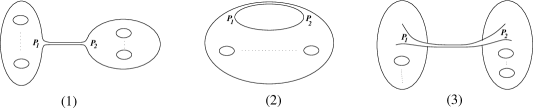
Figure 4: The three degeneration limits.

1. The first degeneration arises when the surface splits into two Riemann surfaces $\Sigma_{(0,h_{1})}$ and $\Sigma_{(0,h_{2})}$ (where $h=h_{1}+h_{2}-1$ and $h_{1},h_{2}\geq 2$) with one puncture each, say $P_{1}$ and $P_{2}$, at the boundaries of the two surfaces. The original anti-chiral insertion $\Phi_{\bar{i}}^{-}$ is on one of the components, say $\Sigma_{(0,h_{1})}$. Since the total charge (i.e. left plus right $U(1)$ charge) on a disk in the twisted theory, as dictated by the $U(1)$ anomaly, should be +3, it follows that the open string insertion at $P_{1}$ carries charge +2, while the open string insertion at $P_{2}$ is its metric-dual operator $\phi_{j}^{+}$ carrying charge +1. The charge +2 state is obtained now by the action of $\rho_{L}+\rho_{R}$ on a charge $-1$ operator. The leftover $3(h-2)-1$ (left plus right) $G^{-}$’s folded with the Beltrami differentials distribute themselves on $\Sigma_{(0,h_{1})}$ and $\Sigma_{(0,h_{2})}$. Their numbers on the two surfaces are respectively $3(h_{1}-2)+1$ and $3(h_{2}-2)+1$ which is dictated by the $U(1)$ charge anomalies on the two surfaces, as well as by the dimension of the moduli space of the corresponding one punctured Riemann surfaces. The resulting term is

   $$F^{(0,h_{1})}_{\bar{i},\bar{j}}G^{\bar{j}j}D_{j}F^{(0,h_{2})};~{}~{}~{}~{}~{}h_{1}+h_{2}=h+1\,.$$ (4.6)

2. The second open string degeneration is analogous to the handle degeneration of the closed string and results in twice-punctured surface $\Sigma_{(0,h-1)}$ with punctures $P_{1}$ and $P_{2}$ on a boundary with the intermediate states at the two punctures carrying charge +2 and +1 respectively. The dimension of this twice-punctured moduli space is $3(h-3)+2$ which is exactly the number of the leftover $G^{-}$’s. This is also in agreement with the total $U(1)$ charge anomaly. The resulting term is

   $$C^{j\bar{j}}D_{j}F^{(0,h-1)}_{\bar{i},\bar{j}}\,.$$ (4.7)

3. Finally there is also a degeneration with closed string intermediate state when the surface splits into $\Sigma_{(0,h_{1})}$ and $\Sigma_{(0,h_{2})}$ with one puncture each $P_{1}$ and $P_{2}$ in the interior of the two surfaces. It is easy to see that $h_{1}+h_{2}=h$ (where now $h_{1},h_{2}\geq 1$). The plumbing fixture coordinate $\tau$ is now complex and the boundary corresponds to $t=|\tau|\to\infty$. Thus the angular part of $\tau$ is still to be integrated. The moduli space of the two surfaces with one puncture each in the interior of the surfaces is $3(h_{1}-2)+2$ and $3(h_{2}-2)+2$ real dimensional, respectively, implying that as many $G^{-}$’s are distributed on the two surfaces, respectively. The remaining one $G^{-}$ is sitting at the node which is folded with the Beltrami differential corresponding to the angular part of $\tau$. Now the question is what are the $U(1)$ charges carried by the closed string intermediate state at $P_{1}$ and $P_{2}$. Since the $U(1)$ anomaly for a sphere (which is the relevant surface for the intermediate closed string propagation) is +6, we conclude that the sum of the $U(1)$ charges at $P_{1}$ and $P_{2}$ is +6. If $\phi_{\bar{i}}^{-}$ is on the first surface, then there are two possibilities: the charges at $(P_{1},P_{2})$ are $(+4,+2)$ or $(+3,+3)$. The charges here are the sum of the left and right moving parts. Charge +4 therefore means (left, right) (anti-chiral, anti-chiral) closed string state where the left and right charge +3 operators $\rho_{L}$ and $\rho_{R}$ have been applied on the anti-chiral operators to convert them into charge +2 operators. Charge +2 operator is the (chiral, chiral) state and hence represents the holomorphic derivative with respect to the corresponding target space modulus. Charge +4 and +2 therefore correspond to the antiholomorphic and holomorphic complex structure moduli, respectively, of the target space. Recall that here we work in the Type I description, where the relevant topological twist is the one of B-model. We thus obtain a term similar to (4.6):

   $$F^{(0,h_{1})}_{\bar{i},\bar{j}}G^{\bar{j}j}D_{j}F^{(0,h_{2})};~{}~{}~{}~{}~{}h_{1}+h_{2}=h\,,$$ (4.8)

   where $j$ and $\bar{j}$ are closed string states.

   Finally, charge +3 at a puncture corresponds to the diagonal combination of (chiral, anti-chiral) plus (anti-chiral, chiral) states which are in fact the Kähler moduli of the target space. These moduli are expected to decouple from the topological B-model. In the Type I context, they are complexified with Ramond-Ramond (RR) fields which are associated with continuous shift symmetries in perturbation theory that make the holomorphic dependence on the Kähler moduli trivial. Charge +3 can also include the identity operator corresponding to exchange of dilaton in the parent string theory. Indeed, in the example discussed in the section 8, there will be such a contribution to the holomorphic anomaly from the identity channel in the closed string degeneration.

Note that for $h=2$ the first type of degeneration is absent, while the second gives the well known holomorphic anomaly equation for the gauge couplings. The terms arising from the degeneration with closed string intermediate states need to be understood further, however in the following we will focus on the terms coming from the first two types of degenerations that involve open string intermediate states. The new terms that appear in the holomorphic anomaly equations are $F^{(0,h)}_{n}$’s, that is $F^{(0,h)}_{\bar{i}_{1}...\bar{i}_{n};\bar{j}_{1}...\bar{j}_{n}}$ where $\bar{i}$ indices refer to open string insertions of anti-chiral operators carrying charge -1 while $\bar{j}$ indices refer to anti-chiral operators carrying charge +2 (by the action of $\rho$). In heterotic theory, it was shown that these quantities originate from F-terms of the form $({\rm Tr}W^{2})^{h}\Pi^{n}$ [5]. In components they include terms like ${\cal F}^{2}(\lambda^{2})^{h-1}\prod_{k=1}^{n}(\psi_{\bar{i}_{k}}.\psi_{\bar{j}_{k}})$ among others, where $\lambda$ are the gauginos and $\psi$ are non-chiral matter fermions. The proof of this statement in the case of open string is identical to the one given for the heterotic case, since in the open string, by going to the double cover, the spin structure sum boils down to just one sector, as in the heterotic string. When supersymmetry is broken by a D-term expectation value, the one-loop term $\Pi{\rm Tr}W^{2}$ gives rise to fermion masses similar to a “Higgs” $\mu$-term in the effective field theory. These masses will be studied in section 7.

5 $F^{(0,3)}$ in Type I with Magnetized D9 Branes

In this section, we consider an explicit example of Type I string compactified on a factorized six-torus $T^{6}=(T^{2})^{3}$, with magnetized D9 branes. We will then compute the topological partition function $F^{(0,3)}$ on a world-sheet with three boundaries, in a $N=1$ supersymmetric configuration corresponding to an appropriate choice of the magnetic fields. For this purpose, we first recall the main properties of the relevant Riemann surface $(g=0,h=3)$.

5.1 Properties of the $(g=0,h=3)$ Riemann surface

The $(g=0,h=3)$ surface $\Sigma_{(0,3)}$ can be obtained from the double torus of genus 2, by applying the world-sheet involution (2.1) exchanging left and right movers, as described in section 2 and shown in Fig. 5.

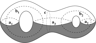
Figure 5: The $(g=0,h=3)$ surface $\Sigma_{(0,3)}$ is in the upper half of its $g=2$ double-cover. ${\bf c}$ is the dividing geodesics.

The period matrix $\tau$, invariant under the involution, is purely imaginary:

$$\tau=i\left(\begin{matrix}t_{11}&t_{12}\cr t_{12}&t_{22}\cr\end{matrix}\right)\,,$$ (5.1)

where $t_{ij}$ are three real parameters, dual to the sizes of the three holes. They correspond to the proper time variables of the closed string propagation channels.

The “relative modular group”, defined by the modular transformations $Sp(4,\mathbb{Z})$ that preserve the involution (2.1), is the group $GL(2,\mathbb{Z})$ [10]. It transforms the period matrix as:

$$\tau\to D\,\tau\,D^{T}\,,$$ (5.2)

where $D$ is an arbitrary $2\times 2$ matrix with an inverse of integer entries. This group, however, in general transforms the boundaries (fixed under the involution) to linear combinations of the boundaries. The relevant modular transformations are the ones that act at most as permutations of the boundaries. This group is generated by

$$D_{1}=\left(\begin{matrix}0&1\cr 1&0\cr\end{matrix}\right)\qquad D_{2}=\left(\begin{matrix}-1&-1\cr 0&1\cr\end{matrix}\right)$$ (5.3)

corresponding to

$$D_{1}:t_{11}\leftrightarrow t_{22}\qquad D_{2}:\left(\begin{matrix}t_{11}\to t_{11}+t_{22}+2t_{12}\cr t_{12}\to-t_{12}-t_{22}\end{matrix}\right)\,.$$ (5.4)

It is easy to see that $D_{1}^{2}=D_{2}^{2}=(D_{1}D_{2})^{3}=1$.

Using the above transformations and the positivity of the period matrix, one can choose as fundamental domain of integration the ordering:

$$-{\sqrt{t_{11}t_{22}}}\leq t_{12}\leq 0\leq t_{11}\leq t_{22}<\infty\,.$$ (5.5)

The three degeneration limits, described in section 4, correspond to the following boundaries of the fundamental domain:

1. $t_{12}\to 0$, corresponding to shrinking the dividing geodesics of genus 2. Then $\Sigma_{(0,3)}$ degenerates to a product of two annuli with one common boundary stretched in the two annuli through a massless open string. Moreover, the period matrix becomes diagonal with $t_{11}$ and $t_{22}$ the closed string proper times of the two annuli.

2. $t_{12}\to-{\sqrt{t_{11}t_{22}}}$, implying the vanishing of the period matrix determinant. In this limit, $\Sigma_{(0,3)}$ degenerates into an annulus with a massless open string attached at one of its boundaries. It amounts to taking the infrared limit of one of the two gauge loops in the effective field theory. Then $t_{22}$ is the proper time of the annulus in the closed string channel while $t_{11}$ parameterizes the length of the open string.

3. $t_{22}\to\infty$, corresponding to pinching an intermediate closed string connecting an annulus with a disk. Then $t_{11}$ becomes the proper time of the annulus in the closed string channel and $t_{12}$ parameterizes the position of the shrinking hole.

5.2 Partition functions

We now discuss the bosonic and fermionic partition functions. Quantum determinants can be obtained by taking the appropriate square root of the corresponding expression on the genus 2 double cover. In the bosonic case, there is a correction factor $R_{\Sigma}$ that depends on the involution and on the boundary conditions [10]. It is given by Eq.(2.16), as described in section 2. In the case of a compact boson, one has to multiply the quantum determinant with the lattice sum of momenta or winding modes (2.13). The resulting partition function for N boundary conditions reads:

$$Z_{B}=Z_{1}^{-1/2}Z^{N,D}_{\rm cl}\qquad Z^{N}_{\rm cl}=R\sum_{\vec{n}}e^{-\displaystyle{\pi R^{2}\over 2}{\vec{n}}t{\vec{n}}^{T}}\,,$$ (5.6)

where ${\vec{n}}=(n_{1},n_{2})$ are the winding numbers around the two $\bf a$ cycles. In the degeneration limit $t_{22}\to\infty$, non-vanishing $n_{2}$ windings are exponentially suppressed, and for $n_{2}=0$ one recovers the annulus partition function depending on the closed string proper time $t_{11}$. The $t_{12}$ dependence, corresponding to the position of the shrinking boundary, drops. Similarly, in the case of D boundary conditions, one has:

$$Z^{D}_{\rm cl}=R(\det t)^{-1/2}\sum_{\vec{m}}e^{-\displaystyle 2\pi R^{2}{\vec{m}}t^{-1}{\vec{m}}^{T}}\,.$$ (5.7)

The method of section 2 can also be applied to the fermionic determinants giving rise to theta functions. The partition function of a complex fermion depends on 16 spin structures corresponding to the four boundary conditions ${\vec{a}}=(a_{1},a_{2})$ and ${\vec{b}}=(b_{1},b_{2})$ around the non-trivial cycles ${\bf a}_{i}$ and ${\bf b}_{i}$:

$$Z_{f}\left[{{\vec{a}}\atop{\vec{b}}}\right] = Z_{1}^{-1/2}\Theta\left[{{\vec{a}}\atop{\vec{b}}}\right](t)$$

$$= Z_{1}^{-1/2}\sum_{{\vec{n}}=(n_{1},n_{2})}e^{\displaystyle-\pi({\vec{n}}+{\vec{a}})t({\vec{n}}+{\vec{a}})^{T}+2i\pi({\vec{n}}+{\vec{a}}){\vec{b}}^{T}}\,.$$

The partition function involves a sum over spin structures with appropriate coefficients $c\left[{{\vec{a}}\atop{\vec{b}}}\right]$, determined at one loop level. As usually, at higher loops the corresponding coefficients are determined by the factorization properties of the vacuum amplitude. Indeed, by considering the factorization limit $t_{12}\to 0$, we find:

$$c\left[{{\vec{a}}\atop{\vec{b}}}\right]=c_{A}\left({a_{1}\atop b_{1}}\right)\ c_{A}\left({a_{2}\atop b_{2}}\right)\,,$$ (5.9)

where $c_{A}$ denote the corresponding coefficients in the annulus amplitude.

5.3 The topological amplitude

We consider now a toroidal compactification of Type I string theory on three factorized tori, $T^{6}=\prod_{I=3,4,5}T^{2}_{I}$, and a $N=1$ supersymmetric configuration of magnetized D9 branes. Since the string diagram has three boundaries, we consider in general three brane stacks associated to the gauge group $U(N_{a})$, $a=1,2,3$. In each of the three abelian factors, there is an internal magnetic field $H_{a}^{I}$ with components along the three factorized tori $T^{2}_{I}$, $I=3,4,5$. They are quantized in units of the corresponding areas ${\sqrt{G}}_{I}$, with $G_{I}$ the determinant of the $T^{2}_{I}$ metric, according to the Dirac quantization condition $H_{a}^{I}=q_{a}^{I}/p_{a}^{I}{\sqrt{G}}_{I}$, where $q_{a}^{I}$ is the respective magnetic flux and $p_{a}^{I}$ the wrapping number of the $a$-th brane around the $I$-th 2-torus. Note that for each $I$ and $a$, the two integers $p_{a}^{I}$ and $q_{a}^{I}$ are relatively coprime. By T-dualizing three directions, one from each $T^{2}$, one obtains an equivalent description as a Type IIA orientifold with D6 branes at angles related to the magnetic fields [7]. More precisely the angle of each brane relative, for instance, to the horizontal axis of $T^{2}_{I}$ is $\theta^{a}_{I}=\arctan H_{a}^{I}\alpha^{\prime}$. In this representation, the condition for having $N=1$ unbroken supersymmetry on the $a$-th stack takes the simple form that the sum of the corresponding angles in the three tori should vanish: $\theta^{a}_{3}+\theta^{a}_{4}+\theta^{a}_{5}=0$.

Let us compute now the topological partition function $F^{(0,3)}$ given by the physical amplitude involving two gauge fields on one of the 3 boundaries and two gauginos on another, associated to the effective F-term interaction $({\rm Tr}W^{2})^{2}$. From the above discussion, it is clear that the computation is just a particular case of the general orbifold compactification described in section 3. Indeed, all twists around a cycles are trivial, while the angles $\theta^{a}_{I}$ related to the magnetic fields play exactly the role of the orbifold twists around the $\bf b$ cycles, as mentioned already in section 3. By identifying the first two boundaries $a=1,2$ with the two ${\bf a}_{i}$ cycles, $i=1,2$, of the homology basis of the genus 2 Riemann surface, and the third boundary $a=3$ with the middle “horizontal” cycle, see Fig. 5, one has the relations:

$$2\pi h_{I}^{1}=2(\theta^{1}_{I}-\theta^{3}_{I})\qquad;\qquad 2\pi h_{I}^{2}=2(\theta^{3}_{I}-\theta^{2}_{I})\,,$$ (5.10)

where $h_{I}^{i}$ are the orbifold twists around the two ${\bf b}_{i}$ cycles.

Using the identification (5.10), the calculation goes along the lines of section 3 and the result is given by (3.14). In section 3, we had not specified the lattice sum involved explicitly. In the Appendix, we give the detailed derivation of the lattice sums appearing in $F^{(0,h)}$ in the example of magnetized D9 branes. Here we just summarize the result for $h=3$. In the T-dual version, the three stacks of D6 branes on the three boundaries, will be parallel to some primitive lattice vectors in each plane, $\vec{v}^{I}_{a}$, where $a$ labels the three boundaries and $\vec{v}^{I}$ are the two dimensional lattice vectors in the $I$-th plane. Since we are considering factorized torii, it is sufficient to focus on one plane, therefore in the following we will drop the index $I$ labeling the different planes. In the final formulae we will reinstate the index $I$. In terms of the magnetic fluxes in the original D9 branes, these vectors are $\vec{v}_{a}=(p_{a}R_{1},q_{a}R_{2})$ where $R_{1}$ and $R_{2}$ are the two radii in that plane in the T-dual theory with intersecting branes. The world-sheet can therefore carry windings $n_{a}\vec{v}_{a}$ on the $a$-th boundary with integer $n_{a}$. However they satisfy the constraint that the sum of the windings over the three boundaries must vanish since it gives the winding on a homologically trivial cycle:

$$\sum_{a=1}^{3}n_{a}\vec{v}_{a}=0\,.$$ (5.11)

Since we are excluding the case when the three stacks of branes are parallel to each other in one or more planes (otherwise there would be enhanced supersymmetry), only one of the $n_{a}$’s is independent and it spans a sublattice of integers that depends on the magnetic flux data $p_{a}$ and $q_{a}$. Thus we have a one-dimensional sublattice sum labeled by, say, $n_{1}$.

On the world-sheet there is another set of integers which appears because the position of different stacks of branes is defined only modulo transverse lattice vectors. Since not all the branes are parallel, we can choose the intersection of two stacks of branes as the origin of the plane. Then the freedom is only in choosing the transverse position of the third stack of branes. Thus we have again a one dimensional lattice sum. Upon Poisson resummation over this lattice we will get a lattice of momenta along the Dirichlet directions of the 3 stacks of branes. The details are given in the Appendix, but here we just give a simple argument to determine what this lattice sum would be. Let $*\vec{v}_{a}$ be the two dimensional dual of $\vec{v}_{a}$ and let ${\sqrt{G}}$ be the area of the torus (i.e. $R_{1}R_{2}$). Then $*\vec{v}_{a}/{\sqrt{G}}$ is the primitive vector in the intersection of the dual momentum lattice and the Dirichlet direction to the $a$-th stack of branes. Thus the boundary state of the $a$-th branes would carry momentum vectors $k_{a}*\vec{v}_{a}/{\sqrt{G}}$ with $k_{a}$ being integers. Conservation of the total momentum gives the same constraint as (5.11) with $n_{a}$ replaced by $k_{a}$.

$$\sum_{a=1}^{3}k_{a}\vec{v}_{a}=0\,.$$ (5.12)

This results in again a one dimensional sublattice sum labeled by say $k_{1}$.

The modular group $SL(2,\mathbb{Z})$, associated to the Kähler modulus of $T^{2}$, acts on the pair of integers $(n_{1},k_{1})$ in the usual way. Since $(n_{1},k_{1})$ span only a sublattice of integers subject to the constraint (5.11) and (5.12), one might wonder if only a subgroup of the full $SL(2,\mathbb{Z})$ survives. However these two constraints are invariant under the full $SL(2,\mathbb{Z})$ symmetry which implies that the symmetry group is indeed the full $SL(2,\mathbb{Z})$.

To proceed further we need to write a classical solution (before the Poisson resummation) carrying the above winding numbers and the transverse positions. In terms of the complex coordinate of the plane $Z=X_{1}+iX_{2}$, the boundary conditions imply that $Z$ is untwisted along the ${\bf a}$ cycles and twisted by say $g_{1}=e^{2i\pi h^{1}}$ and $g_{2}=e^{2i\pi h^{2}}$ along the ${\bf b}_{1}$ and ${\bf b}_{2}$ cycles of the genus 2 double cover of the surface $\Sigma_{(0,3)}$. Denoting by $\{g\}$ the collection of the twists $g_{1}$ and $g_{2}$, we note that by Riemann-Roch theorem there is only one linearly independent holomorphic twisted differential (Prym Differential) $\omega_{\{g\}}$. To write the classical solution we need the twisted holomorphic differentials $\omega_{\{g\}}$, $\omega_{\{g^{-1}\}}$ and their complex conjugates $\bar{\omega}_{\{g\}}$, $\bar{\omega}_{\{g^{-1}\}}$. The solution is of the form

$$Z(P)=L\int_{P_{0}}^{P}\omega_{\{g\}}+\tilde{L}\int_{P_{0}}^{P}\bar{\omega}_{\{g^{-1}\}}\,,$$ (5.13)

where $L$ and $\tilde{L}$ are determined in terms of winding number and transverse position data and the normalization condition for the twisted differential. Since ${\bf a}$ cycles are untwisted, we can choose the normalization condition (for convenience)

$$\int_{{\bf a}_{1}}\omega_{\{g\}}=g_{1}^{1/2}\,.$$ (5.14)

Note that the integral around $a_{2}$ cycle is not independent since integrating over the trivial cycle $\prod_{i=1}^{2}({\bf a}_{i}{\bf b}_{i}{\bf a}_{i}^{-1}{\bf b}_{i}^{-1})$ gives the constraint

$$[(1-g_{1})\int_{{\bf a}_{1}}+(1-g_{2})\int_{{\bf a}_{2}}]\omega_{\{g\}}=0.$$ (5.15)

By using Fig. 6 (for $h=3$), one can evaluate

$$\int_{\Sigma_{(0,3)}}\omega_{\{g\}}\wedge\bar{\omega}_{\{g\}}=\tau_{\{g\}}-\bar{\tau}_{\{g\}}~{}~{}~{};~{}~{}~{}~{}\tau_{\{g\}}=D_{\{g\}}+\frac{1}{2}\frac{(1-g_{1})(1-g_{2}g_{1}^{-1})}{1-g_{2}}\,,$$ (5.16)

where

$$D_{\{g\}}=2i\frac{(g_{1}g_{2})^{-\frac{1}{2}}}{1-g_{2}^{-1}}\int_{{\bf b}_{1}{\bf b}_{2}{\bf b}_{1}^{-1}{\bf b}_{2}^{-1}}\omega_{\{g\}}\,.$$ (5.17)

Note that the individual cycles ${\bf b}_{i}$ are not closed due to the twists, but the cycle ${\bf b}_{1}{\bf b}_{2}{\bf b}_{1}^{-1}{\bf b}_{2}^{-1}$ is closed. Due to the symmetry of the double cover under the involution (2.1), $D$ turns out to be purely imaginary. By using the identity $\int_{\Sigma_{(0,3)}}\omega_{\{g\}}\wedge{\omega}_{\{g^{-1}\}}=0$ we have the relation $\tau_{\{g\}}=\tau_{\{g^{-1}\}}$.

The final result of the lattice contribution as shown in the Appendix (including all the three planes) is

$$Z_{\rm lattice}=\prod_{I}p_{I}\left({{\rm Im}\tilde{\tau}_{\{g_{I}\}}\over{\rm Im}T}\right)^{1/2}\sum_{(n^{I}_{1},k^{I}_{1})}e^{2i\pi(n^{I}_{1}\alpha^{I}_{1}+k^{I}_{1}\alpha^{I}_{2})}e^{\frac{i\pi}{{\rm Im}T_{I}}|n^{I}_{1}T_{I}+k^{I}_{1}|^{2}\tilde{\tau}_{\{g_{I}\}}}\,,$$ (5.18)

where $T_{I}=B_{I}+i{\sqrt{G}}_{I}$ is the usual Kähler modulus of the torus $T^{2}_{I}$, with $B_{I}$ the two-index antisymmetric tensor. The parameter $\tilde{\tau}_{\{g_{I}\}}=\frac{|v^{I}_{1}|^{2}}{{\rm Im}T_{I}}\tau_{\{g_{I}\}}$ is independent of the modulus $T_{I}$, although it depends on the world-sheet moduli and the flux data. Furthermore, $\alpha_{1}$ is the effective Wilson line along the world-volume of the branes and $\alpha_{2}$ is the effective transverse position of the branes (which is T-dual to the second component of the Wilson line in the D9 brane theory). The integer $p_{I}$ is the smallest positive integer such that

$$p_{I}\frac{v_{3}^{I}.*v_{1}^{I}}{v_{3}^{I}.*v_{2}^{I}}\in\mathbb{Z}.$$ (5.19)

Note that the above equation implies

$$p_{I}\frac{v_{2}^{I}.*v_{1}^{I}}{v_{3}^{I}.*v_{2}^{I}}\in\mathbb{Z}.$$ (5.20)

From the constraints (5.11) and (5.12) it follows that $n_{1}^{I}$ and $k_{1}^{I}$ are arbitrary integer multiples of $p_{I}$. As observed in subsection 5.1 [preceding Eq.(5.4)], the relevant modular group is the permutation group $S_{3}$ that permutes the three boundaries. Since we have treated the three boundaries asymmetrically in arriving to Eq.(5.18), it is not manifest that the result is modular invariant. For example, we have normalized the Prym differential along the first boundary and the lattice momenta appearing in the expression refer directly to the boundary state of the brane attached to this boundary. Indeed, under the permutation of the boundaries, $\tau_{\{g_{I}\}}$, $p_{I}$ and $|v_{1}^{I}|$ transform nontrivially. However, the combination $p_{I}|v_{1}^{I}|\tau_{\{g_{I}\}}^{\frac{1}{2}}$ is invariant. For instance, under the exchange of first and second boundaries,

$$v_{1}^{I}\to v_{2}^{I},\qquad p_{I}\to p_{I}\left|\frac{v_{3}^{I}.*v_{2}^{I}}{v_{3}^{I}.*v_{1}^{I}}\right|\quad~{}\makebox{and}~{}\quad\tau_{\{g_{I}\}}\to\left|\frac{1-g_{1}^{I}}{1-g_{2}^{I}}\right|^{2}\tau_{\{g_{I}\}}.$$ (5.21)

The latter can be seen by the fact that under the exchange of ${\bf a}_{1}$ and ${\bf a}_{2}$ cycles, $\omega_{\{g_{I}\}}$ [normalized by Eq.(5.14) around ${\bf a}_{1}$ cycle], is transformed to $-\frac{1-g_{1}^{I}}{1-g_{2}^{I}}\omega_{\{g_{I}\}}$, where we used the constraint (5.15). The statement that $p_{I}|v_{1}^{I}|\tau_{\{g_{I}\}}^{\frac{1}{2}}$ is invariant now follows from the relation

$$\left|\frac{1-g_{1}^{I}}{1-g_{2}^{I}}\right|=\left|\frac{v_{3}^{I}.*v_{1}^{I}}{v_{3}^{I}.*v_{2}^{I}}\right|\frac{|v_{2}^{I}|}{|v_{1}^{I}|}.$$ (5.22)

As a result, $Z_{\rm lattice}$ as given in (5.18) is invariant under the permutation group.

In the topological partition function, we have also the insertion of $G^{-}$’s which are folded with the Beltrami differentials. As mentioned earlier, each $\bar{\psi}^{I}$ field, being of dimension 1 in the topological theory, has now only one zero mode (for each plane $I$). It will therefore be replaced by $\omega_{\{g_{I}^{-1}\}}$. Similarly $\partial Z_{I}$ will be replaced by the zero mode

$$\partial Z_{I}=\frac{v_{I}}{{\rm Im}T_{I}}(n^{I}_{1}T_{I}+k^{I}_{1})\omega_{\{g_{I}\}}\,.$$ (5.23)

Integrating the fermion zero modes we get

$$\prod_{a=1}^{3}\int\mu_{a}G^{-}=\prod_{I=1}^{3}\frac{v_{I}}{{\rm Im}T_{I}}(n^{I}_{1}T_{I}+k^{I}_{1})\det\int\mu_{a}h_{J}\quad;\quad h_{J}=\omega_{\{g_{J}\}}\omega_{\{g_{J}^{-1}\}}\,.$$ (5.24)

We can further evaluate the determinant above by noting that under the deformation of the complex structure represented by the Beltrami differential $\mu_{a}$, the twisted $(1,0)$ form $\omega_{\{g_{I}\}}$ picks up a $(0,1)$ form given by

$$\omega_{\{g_{I}\}}\rightarrow\omega_{\{g_{I}\}}+C\bar{\omega}_{\{g^{-1}_{I}\}}\quad;\quad C\bar{\omega}_{\{g^{-1}_{I}\}}=\mu_{a}\omega_{\{g_{I}\}}\ ~{}~{}{\rm modulo\ an\ exact\ form}\,.$$ (5.25)

As a result

$$\int\mu_{a}\omega_{\{g_{I}\}}\omega_{\{g^{-1}_{I}\}} = C\int\bar{\omega}_{\{g^{-1}_{I}\}}\omega_{\{g^{-1}_{I}\}}$$ (5.26)

$$= C(\tau_{\{g_{I}\}}-\bar{\tau}_{\{g_{I}\}}).$$

Now we will relate this to the variation of the twisted $\tau_{\{g_{I}\}}$. The moduli dependent part of the latter, as seen from Eq.(5.16) and (5.17), is proportional to the ratio of the periods $\int_{{\bf b}_{1}{\bf b}_{2}{\bf b}_{1}^{-1}{\bf b}_{2}^{-1}}\omega_{\{g_{I}\}}/\int_{{\bf a}_{1}}\omega_{\{g_{I}\}}$. From the variation of the twisted differential given in (5.25) we find

$$\delta_{a}\tau_{\{g_{I}\}} = C(\bar{D}_{\{g_{I}^{-1}\}}-D_{\{g_{I}\}})$$ (5.27)

$$= C(\tau_{\{g_{I}\}}-\bar{\tau}_{\{g_{I}\}})$$

$$= \int\mu_{a}\omega_{\{g_{I}\}}\omega_{\{g^{-1}_{I}\}}\,,$$

where in the second equality we have used Eqs.(5.16) and (5.17) and the fact that $\tau_{\{g_{I}\}}=\tau_{\{g_{I}^{-1}\}}$. The determinant appearing in (5.24) therefore just gives the Jacobian of the transformation from the moduli to $\tau_{\{g_{I}\}}$. If the latter, for $I=3,4,5$ are independent functions on the moduli space, then the Jacobian is non-vanishing and the resulting measure of integration on the moduli space becomes $\prod_{I}d\tau_{\{g_{I}\}}$.

In the topological twisted theory the non-zero modes of the bosons and fermions cancel leaving only the correction factor coming from the boundary conditions on the bosons discussed in section 2 and summarized in Eq.(2.16). For the twisted bosons, $\tau$ in (2.16) is replaced by the corresponding twisted $\tau$. The resulting ${\rm det}\tau$ factor cancels the one appearing in lattice partition function (5.18).

The above calculations were done in the D6 brane theory. By T-dualizing we can go to the magnetized D9 brane theory. This amounts to replacing $T_{I}\to U_{I}$ and ${\rm Im}U_{I}\to{\rm Im}T_{I}=\sqrt{G_{I}}$. Here, $U$ is the usual complex structure modulus of the torus $T^{2}$, given in terms of its metric $G_{ij}$, $i,j=1,2$: $U=(G_{12}+i{\sqrt{G}})/G_{11}$. The resulting topological partition function becomes:

$$F^{(0,3)}=3N\int\prod_{I=3}^{5}d\tilde{\tau}_{\{g_{I}\}}p^{I}f\left[U_{I},\vec{\alpha}_{I};-i\tilde{\tau}_{\{g_{I}\}}\right]\,,$$ (5.28)

where the integration variables

$$\tilde{\tau}_{\{g_{I}\}}=\sqrt{G_{I}}(p_{1}^{I})^{2}\left[1+(H^{I}_{1})^{2}\right]\tau_{\{g_{I}\}}\,.$$ (5.29)

Here $H^{I}_{a}=\frac{q^{I}_{a}}{p^{I}_{a}\sqrt{G_{I}}}$ is the magnetic field on the $a$-th brane stack in the $I$-th plane. The function $f$ is given by:

$$f(U,\vec{\alpha},l)=\frac{1}{{\rm Im}U}\sum_{n_{1},n_{2}}(n_{1}+n_{2}\bar{U})e^{2i\pi\vec{n}\cdot\vec{\alpha}}e^{-{\pi\over{\rm Im}U}|n_{1}+n_{2}U|^{2}l}\,,$$ (5.30)

where the lattice sum of integers $\vec{n}^{I}$ for each $I$ satisfy the conditions

$$p^{I}_{1}\vec{n}_{I}+p^{I}_{2}\vec{n}^{\prime}_{I}+p^{I}_{3}\vec{n}^{\prime\prime}_{I}=q^{I}_{1}\vec{n}_{I}+q^{I}_{2}\vec{n}^{\prime}_{I}+q^{I}_{3}\vec{n}^{\prime\prime}_{I}=0$$ (5.31)

for some integer vectors $\vec{n}^{\prime}_{I}$ and $\vec{n}^{\prime\prime}_{I}$. $\vec{\alpha}_{I}$ is the Wilson line in the $I$-th plane and is given in terms of a certain linear combination of the Wilson lines on the three brane stacks:

$$\vec{\alpha}^{I}=\vec{\alpha}^{I}_{1}-\frac{p^{I}_{3}q^{I}_{1}-q^{I}_{3}p^{I}_{1}}{p^{I}_{3}q^{I}_{2}-q^{I}_{3}p^{I}_{2}}\vec{\alpha}^{I}_{2}+\frac{p^{I}_{2}q^{I}_{1}-q^{I}_{2}p^{I}_{1}}{p^{I}_{3}q^{I}_{2}-q^{I}_{3}p^{I}_{2}}\vec{\alpha}^{I}_{3}\,,$$ (5.32)

where the subscripts $1,2,3$ refer to the three different stacks of branes on the three boundaries of the world-sheet. Obviously, the result vanishes for ${\vec{\alpha}_{I}}=0$ for any $I$, due to the ${\vec{n}}_{I}\to-{\vec{n}}_{I}$ symmetry of the lattice sum. Note that non-trivial $\vec{\alpha}_{I}$, although breaks the corresponding R-symmetry, does not change the spectrum. The positive integers $p_{I}$ appearing in (5.28) satisfy (5.19) which can be reexpressed in terms of the flux data as $p_{I}$ being the smallest positive integer such that

$$p_{I}\frac{p^{I}_{3}q^{I}_{1}-q^{I}_{3}p^{I}_{1}}{p^{I}_{3}q^{I}_{2}-q^{I}_{3}p^{I}_{2}}\in\mathbb{Z}~{}~{}~{}\Rightarrow~{}~{}~{}p_{I}\frac{p^{I}_{2}q^{I}_{1}-q^{I}_{2}p^{I}_{1}}{p^{I}_{3}q^{I}_{2}-q^{I}_{3}p^{I}_{2}}\in\mathbb{Z}\,.$$ (5.33)

It is worth making some comments on the topological partition function (5.28). The first comment is regarding modular invariance. From the constraint (5.31) it follows that $n_{1}^{I}$ and $n_{2}^{I}$ are arbitrary integer multiples of $p_{I}$. The discussion following Eq.(5.19) then implies that (5.28) is invariant under the permutation of the boundaries.

The second comment is regarding the target space duality properties of (5.28). We have already mentioned that it has full $SL(2,\mathbb{Z})_{U}$ symmetry despite the fact that the sum is over a sublattice defined by the constraints (5.31). This is because the constraints are $SL(2,\mathbb{Z})_{U}$ covariant. As for the monodromy under shifts of the Wilson lines we note that the constraints imply that ${\vec{n}}_{I}\in p^{I}{\vec{Z}}_{I}$ where ${\vec{Z}}$ is a two-dimensional vector with arbitrary integer components. It follows then that $F^{(0,3)}$ is invariant under shifts $\vec{\alpha}_{I}\to\vec{\alpha}_{I}+\vec{Z}_{I}/p_{I}$.

The topological partition function (5.28) appears deceptively simple as products of three separate integrals, however, the domain of integration over ${\tilde{\tau}}_{\{g_{I}\}}$ is very complicated and in general mixes the three integrals. There are some comments worth making about $F^{(0,3)}$:

• Taking derivatives with respect to anti-holomorphic moduli should result in a total derivative in the world-sheet moduli space, as follows from the general discussion of section 4. The anti-holomorphic moduli in the present case are the complex structure closed string moduli $\bar{U}_{I}$ and the complexified Wilson lines

  $$A_{I}=\alpha_{2}^{I}-U_{I}\alpha_{1}^{I}\,.$$ (5.34)

  The physical quantities are invariant under $A_{I}\rightarrow A_{I}+1/p_{I}$ and $A_{I}\rightarrow A_{I}+U_{I}/p_{I}$. The derivatives with respect to the anti-holomorphic moduli can be easily evaluated using the identities:

  $${\partial f\over\partial{\bar{A}}} = {1\over{\rm Im}U}{\partial Z\over\partial l}\quad;\quad Z={\sum_{n_{1},n_{2}}}e^{2i\pi{\vec{a}}\cdot{\vec{n}}}e^{-{\pi\over{\rm Im}U}|n_{1}+n_{2}U|^{2}l}$$

  $${\partial f\over\partial{\bar{U}}} = -{1\over 4{\rm Im}U}{\partial{(lf)}\over\partial l}\ -\frac{{\rm Im}A}{({\rm Im}U)^{2}}\frac{\partial Z}{\partial l},$$ (5.35)

  which follow from the form of the function $f$ in Eq.(5.30).

• The dependence on the Kähler moduli of the tori, namely $\sqrt{G_{I}}$, should drop out because the complexification of these moduli involve the Ramond-Ramond $B$ fields. Since the latter are associated with continuous shift symmetries in perturbation theory, the dependence on them should be trivial.

6 Gaugino Masses

In this section, we compute the Majorana gaugino masses in the general non-supersymmetric case with the sum of the brane angles different from zero. Using their relation to the orbifold twists (5.10), we parameterize the supersymmetry breaking as

$$\sum_{I=3}^{5}h_{I}=-2\epsilon\,,$$ (6.1)

where for simplicity we dropped the cycle indices. The parameter $\epsilon$ fixes the scalar masses and in the weak field limit $\epsilon\to 0$, it is proportional to the expectation value of the corresponding abelian D-term. In this limit, the gaugino masses are determined from the effective F-term $({\rm Tr}W^{2})^{2}$ and should therefore be identified with the topological partition function $F^{(0,3)}$.

The gaugino vertices in the $-1/2$ ghost picture are given in Eq.(3.1) and are inserted on one of the three boundaries of the $(g=0,h=3)$ Riemann surface. Moreover one has to insert three picture changing operators $e^{\varphi}T_{F}$, which we also choose to be on the boundaries. One of them is needed to change the ghost picture of one gaugino to $+1/2$, while the other two arise from the integration over the supermoduli:

$$m_{1/2}=g_{s}^{2}\int[dt]\int dxdy\ {\cal A}\quad;\quad{\cal A}=\left\langle V^{(-1/2)}_{+}(x)V^{(-1/2)}_{-}(y)\prod_{i=1}^{3}e^{\varphi}T_{F}(z_{i})\right\rangle\,,$$ (6.2)

where $g_{s}$ is the string coupling and its power takes into account the normalization of the gaugino kinetic terms on the disk. The moduli integration is over the fundamental domain (5.5), while $x$ and $y$ are integrated over the gaugino boundary. The dependence on the positions $z_{i}$ of the picture changing operators is a gauge artifact and should disappear from the physical amplitude.

By internal charge conservation, since both gauginos carry charge $+1/2$ for $\phi_{3}$, $\phi_{4}$ and $\phi_{5}$, only the internal part of the world-sheet supercurrents (3.8) contributes; each $T_{F}^{int}$ should provide $-1$ charge for $\phi_{3}$, $\phi_{4}$ and $\phi_{5}$, respectively. The amplitude (6.2) then becomes:

$${\cal A} = \langle e^{-\varphi/2}(x)e^{-\varphi/2}(y)\prod_{I=3}^{5}\!e^{\varphi}(u_{I})\rangle\prod_{I=1}^{2}\!\langle e^{i\phi_{I}/2}(x)e^{-i\phi_{I}/2}(y)\rangle$$ (6.3)

$$\times\prod_{I=3}^{5}\!\langle e^{i\phi_{I}/2}(x)e^{i\phi_{I}/2}(y)e^{-i\phi_{I}}(u_{I})\rangle\,,$$

where $\{u_{I}\}$, $I=3,4,5$, is a permutation of $\{z_{i}\}$, $i=1,2,3$, and an implicit summation over all permutations is understood. Performing the contractions for a given spin structure $s$, one finds:

$${\cal A}_{s} = {\theta_{s}^{2}({1\over 2}(x-y))\prod_{I=3}^{5}\theta_{s,-h_{I}}({1\over 2}(x+y)-u_{I})\,\partial X_{h_{I}}(u_{I})\over\theta_{s}({1\over 2}(x+y)-\sum_{I=3}^{5}u_{I}+2\Delta)}$$ (6.4)

$$\times{\sigma(x)\sigma(y)\over\prod_{I<J}^{3,4,5}E(u_{I},u_{J})\prod_{I=3}^{5}\sigma^{2}(u_{I})}\times{Z_{2}\over Z_{1}^{4}\prod_{I=3}^{5}Z_{1,h_{I}}}Z_{lat}\,,$$

where $\theta_{s}$ is the genus-two theta-function of spin structure $s$, $E$ is the prime form, $\sigma$ is a one-differential with no zeros or poles and $\Delta$ is the Riemann $\theta$-constant. $Z_{1,h_{I}}$ is the (chiral) determinant of the $h_{I}$-twisted $(1,0)$ system, and $Z_{2}$ is the chiral non-zero mode determinant of the $(2,-1)$ b-c ghost system. Finally, $Z_{lat}$ stands for all zero-mode parts of space-time and internal coordinates, while an implicit summation over lattice momenta should be performed, taking into account also the $\partial X_{I}$ factors in (6.4).

In order to perform an explicit sum over spin structures, one should choose the positions of the picture changing operators to satisfy a condition that makes the argument of the $\theta$-function in the denominator equal to $(x-y)/2$, so that one $\theta_{s}$ factor simplifies. The resulting relation however,

$$\sum_{i=1}^{i=3}z_{i}=y+2\Delta\,,$$ (6.5)

is not allowed. To bypass this difficulty, we insert in the amplitude (6.2) another vertex of an open string Wilson line associated to the $I=3$ internal plane, in the $-1$ ghost picture:

$$V^{(-1)}=:e^{-\varphi}\psi_{3}(w):\,,$$ (6.6)

accompanied by a forth picture changing operator at the boundary position $z_{4}$. Obviously, we should also perform a third integration over its position $w$. The new vertex brings another unit of charge for $\phi_{3}$, and thus, two of the four supercurrents should provide $-1$ charge for $\phi_{3}$. As we will demonstrate below, one can now choose an appropriate gauge condition which allows to perform the spin structure sum and show that the amplitude can be written as the variation with respect to the Wilson line of the original one (6.4), evaluated formally using the “forbidden” gauge choice (6.5).

Indeed, the correlators in (6.3) now become:

$${\cal A}\!\!\! = \!\!\!\langle e^{-\varphi/2}(x)e^{-\varphi/2}(y)e^{-\varphi}(w)\prod_{I=3}^{6}e^{\varphi}(u_{I})\rangle\prod_{I=1}^{2}\langle e^{i\phi_{I}/2}(x)e^{-i\phi_{I}/2}(y)\rangle$$

$$\times \!\!\!\langle e^{i\phi_{3}/2}(x)e^{i\phi_{3}/2}(y)e^{i\phi_{3}}(w)\prod_{I=3,6}e^{-i\phi_{3}}(u_{I})\rangle\prod_{I=4,5}\langle e^{i\phi_{I}/2}(x)e^{i\phi_{I}/2}(y)e^{-i\phi_{I}}(u_{I})\rangle\,,$$

where $\{u_{I}\}$, $I=3,\dots,6$, is a permutation of $\{z_{i}\}$, $i=1,2,3,4$, and an implicit summation over all permutations is understood. Performing the contractions, one finds that the expression (6.4) is modified as:

$${\cal A}_{s}\!\!\!\! = \!\!\!\!{\theta_{s}^{2}({1\over 2}(x-y))\theta_{s,-h_{3}}({1\over 2}(x+y)-u_{3}+w-u_{6})\ \!\prod_{I=4,5}\theta_{s,-h_{I}}({1\over 2}(x+y)-u_{I})\over\theta_{s}({1\over 2}(x+y)+w-\sum_{I=3}^{6}u_{I}+2\Delta)}$$

$$\times\,{\sigma(x)\sigma(y)\sigma^{2}(w)\over\prod_{I<J}^{3,4,5}E(u_{I},u_{J})\prod_{I=3}^{6}\sigma^{2}(u_{I})}{E(w,u_{4})E(w,u_{5})\over E(u_{6},u_{4})E(w-u_{6},u_{5})}$$

$$\times\,{Z_{2}Z_{lat}\over Z_{1}^{4}\prod_{I=3}^{5}Z_{1,h_{I}}}\prod_{I=3,6}\partial X_{3,h_{3}}(u_{I})\prod_{I=4,5}\partial X_{I,h_{I}}(u_{I})\,.$$

To perform the spin structure sum, we use the allowed gauge condition:

$$\sum_{i=1}^{i=4}z_{i}=y+w+2\Delta\,.$$ (6.9)

The sum over spin structures converts the first factor in (6) to:

$$\theta_{\epsilon}(x-\Delta)\theta_{h_{3}+\epsilon}(u_{3}+u_{6}-w-\Delta)\theta_{h_{4}+\epsilon}(u_{4}-\Delta)\theta_{h_{5}+\epsilon}(u_{5}-\Delta)\,,$$ (6.10)

where we used Eq.(6.1).

We now use three bosonization formulae. First,

$$\theta_{h_{3}+\epsilon}(u_{3}+u_{6}-w-\Delta){E(u_{3},u_{6})Z_{1}^{-1/2}\over E(u_{3},w)E(u_{6},w)}{\sigma(u_{3})\sigma(u_{6})\over\sigma(w)}$$ (6.11)

$$=\langle{\overline{\psi}}_{h_{3}+\epsilon}(u_{3}){\overline{\psi}}_{h_{3}+\epsilon}(u_{6})\psi_{-h_{3}-\epsilon}(w)\rangle Z_{1,h_{3}+\epsilon}\,,$$

where $\psi$ and $\overline{\psi}$ are conformal fields of dimension zero and one, respectively, twisted as indicated by their subscripts. Then

$$\theta_{h_{I}+\epsilon}(u_{I}-\Delta)\sigma(u_{I})Z_{1}^{-1/2}=\omega_{h_{I}+\epsilon}(u_{I})Z_{1,h_{I}+\epsilon}\,,$$ (6.12)

where $\omega_{h}$ is an abelian differential twisted by $h$. Finally,

$$\theta_{\epsilon}(\sum_{I=3}^{6}u_{I}-w-3\Delta){\prod_{I<J}E(u_{I},u_{J})\over\prod_{I=3}^{6}E(u_{I},w)}{\prod_{I=3}^{6}\sigma^{3}(u_{I})\over\sigma^{3}(w)}Z_{1}^{-1/2}\!\!=\!\!\langle\prod_{I=3}^{6}b_{\epsilon}(u_{I})c_{-\epsilon}(w)\rangle Z_{2,\epsilon},$$ (6.13)

where the correlator and the non-zero mode determinant of the b-c ghost system in the r.h.s. are twisted according to the subscripts.

Multiplying the amplitude (6) by $\theta_{\epsilon}(y-\Delta)/\theta_{\epsilon}(\sum_{I=3}^{6}u_{I}-w-3\Delta)$ which is equal to the identity by our gauge condition (6.9), and using the spin structure sum (6.10) and the bosonization formulae (6.11) - (6.13), we obtain:

$${\cal A} = \theta_{\epsilon}(x-\Delta)\theta_{\epsilon}(y-\Delta)\prod_{I=3}^{5}\left({Z_{1,h_{I}+\epsilon}\over Z_{1,h_{I}}}\right){\langle{\overline{\psi}}_{h_{3}-\epsilon}(u_{3}){\overline{\psi}}_{h_{3}+\epsilon}(u_{6})\psi_{-h_{3}-\epsilon}(w)\rangle\over\langle\prod_{I=3}^{6}b_{\epsilon}(u_{I})c_{-\epsilon}(w)\rangle}$$ (6.14)

$$\times\prod_{I=4,5}\omega_{h_{I}+\epsilon}(u_{I})\sigma(x)\sigma(y){Z_{2}\over Z_{2,\epsilon}}{1\over Z_{1}^{3}}{\prod_{I=3,6}\partial X_{3,h_{3}}(u_{I})\prod_{I=4,5}\partial X_{I}(u_{I})}.$$

Replacing $\omega_{h_{I}+\epsilon}(u_{I})$ by ${\overline{\psi}}_{h_{I}+\epsilon}(u_{I})$ and using the bosonization formula (6.12) twice, one finds:

$${\cal A}={\langle\prod_{i=1}^{4}G^{-}_{\epsilon}(z_{i})\psi_{-h_{3}-\epsilon}(w)\rangle\over\langle\prod_{i=1}^{4}b_{\epsilon}(z_{i})c_{-\epsilon}(w)\rangle}\prod_{I=3}^{5}\left({Z_{1,h_{I}+\epsilon}\over Z_{1,h_{I}}}\right){Z_{2}\over Z_{2,\epsilon}}\left({Z_{1,\epsilon}\over Z_{1}}\right)^{2}\!\!\omega_{\epsilon}(x)\omega_{\epsilon}(y),$$ (6.15)

where $G^{-}_{\epsilon}$ is the internal $N=2$ supercurrent twisted by $\epsilon$.

One can now show that the ratio of correlation functions in (6.15) is independent of the positions $z_{i}$:

$${{\cal N}\over{\cal D}}\equiv{\langle\prod_{i=1}^{4}G^{-}_{\epsilon}(z_{i})\psi_{-h_{3}-\epsilon}(w)\rangle\over\langle\prod_{i=1}^{4}b_{\epsilon}(z_{i})c_{-\epsilon}(w)\rangle}=B_{\epsilon}\partial X_{3,h_{3}}\omega_{-h_{3}}(w)\,,$$ (6.16)

with $B_{\epsilon}$ a constant to be determined. Indeed, as a function of $w$, both numerator ${\cal N}$ and denominator ${\cal D}$ have first order poles when $w\to z_{i}$ with residues $\langle\prod_{i=1}^{3}G^{-}_{\epsilon}(z_{i})\rangle\partial X_{3,h_{3}}$ and $\langle\prod_{i=1}^{3}b_{\epsilon}(z_{i})\rangle$, when for instance $w\to z_{4}$. These are equal, up to a $z_{i}$-independent multiplicative factor $B_{\epsilon}$. Consider now the combination ${\cal N}-B_{\epsilon}\partial X_{3,h_{3}}\omega_{-h_{3}}(w){\cal D}$. This is holomorphic in $w$ twisted 0-form and therefore vanishes identically. Thus, $B_{\epsilon}$ is given by:

$$B_{\epsilon}\omega_{-h_{3}}(w)={\langle\prod_{i=1}^{3}G^{-}_{\epsilon}(z_{i})\rangle\over\langle\prod_{i=1}^{3}b_{\epsilon}(z_{i})\rangle}\,.$$ (6.17)

Note that this is reduced to the same result as the one that would be obtained using the “forbidden” gauge condition (6.5), with an additional differentiation with respect to the Wilson line (6.6) associated to the presence of $\partial X_{3,h_{3}}\omega_{-h_{3}}(w)$ in (6.16).

It follows that the gaugino mass (6.2) is given by:

$$m_{1/2}=g_{s}^{2}\int[dt]B_{\epsilon}\prod_{I=3}^{5}\left({Z_{1,h_{I}+\epsilon}\over Z_{1,h_{I}}}\right){Z_{2}\over Z_{2,\epsilon}}\left({Z_{1,\epsilon}\over Z_{1}}\right)^{2}\,,$$ (6.18)

where we performed the boundary integrals over $x$ and $y$, using the canonical normalization over the $\bf a$-cycles $\int_{\bf a}\omega_{\epsilon}=1$, since $\epsilon$ is a twist around the $\bf b$-cycles. In the limit of small supersymmetry breaking scale $\epsilon\to 0$, one has $Z_{1,\epsilon}\simeq\epsilon Z_{1}$, and thus

$$m_{1/2}\simeq g_{s}^{2}\epsilon^{2}\int[dt]B_{0}=g_{s}^{2}\epsilon^{2}F^{(0,3)}\,.$$ (6.19)

7 $\Pi$-terms and Matter Fermion Masses

In the previous section, we studied the (Majorana) gaugino mass terms generated via D-term supersymmetry breaking. They originate from the supersymmetric F-term $({\rm Tr}W^{2})^{2}$ once the auxiliary D-component of the vector superfield acquires a non-zero VEV along a magnetized $U(1)$ group factor. The corresponding topological coupling is given by $F^{(0,3)}$, with the three boundaries of the world-sheet attached (in a T-dual picture) to three different stacks of D6 branes intersecting at angles in the internal compactification space. In order to get a non-zero answer, we had to further break the discrete R-symmetry by turning on suitable Wilson lines. In the following we analyze the structure of the terms appearing in the holomorphic anomaly equation for $F^{(0,3)}$. The are of the form $\Pi{\rm Tr}W^{2}$, where $\Pi$ is a chiral projection of a non-holomorphic function of chiral superfields. Generically, its lower component includes a fermion bilinear of the form ${\bar{\Psi}}_{\bar{i}}{\bar{\Psi}}_{\bar{j}}$. Hence, upon D-term supersymmetry breaking, they will also induce some fermion masses, in this case of Dirac type.

In order to examine the holomorphic anomaly of $F^{(0,3)}$, we take an anti-holomorphic derivative $\partial_{\bar{i}}$, with respect to an open string Wilson line $\bar{i}$. From the analysis of section 4, one finds contributions from three possible degeneration limits. The two open string degenerations, (1) and (2), involve $F^{(0,2)}_{\bar{i};\bar{j}}$, where $\bar{j}$ denotes an intermediate anti-chiral open string state. In this section, we restrict our discussion to brane configurations that do not involve parallel stacks in any of the three internal planes. This means that in the supersymmetric limit there are no $N=2$ supersymmetric sectors in the one-loop partition function. In the absence of such sectors, the dividing degeneration (1) does not contribute because $\bar{j}$ is an untwisted operator and the corresponding annulus diagrams vanish. In the handle degeneration limit (2) however, since the open string propagating through the handle stretches between two non-parallel brane stacks, it is necessarily twisted. The third degeneration limit (3) involves intermediate closed strings which, in $T^{6}$ compactifications, are always untwisted. Hence, the corresponding annulus diagrams also vanish.

Thus, the only quantity that appears in the holomorphic anomaly of $F^{(0,3)}$ arises from Eq.(4.7), and involves $D_{j}F^{0,2}_{\bar{i};\bar{j}}$, where $j$ and $\bar{j}$ label chiral and anti-chiral twisted open string states with $U(1)$ charges +1 and +2 respectively. These are therefore bi-fundamental states and represent open strings stretched between two different stacks of D6 branes (say $a=1$ and $a=2$) that are not parallel to each other. If the intersection of these two stacks of D6 branes preserves supersymmetry then the twist angles $h_{I}$ in the three internal planes (tori), $I=3,4,5$, satisfy $\sum_{I}h_{I}=1$ and the corresponding twisted states are massless. In the topological theory

$$D_{j}F^{(0,2)}_{\bar{i};\bar{j}}=\int dt^{1}dt^{2}\int dx\langle\left\{\prod_{m=1}^{2}\int\mu_{m}(G_{L}^{-}+G^{-}_{R})\right\}V_{j}(u)V_{\bar{i}}(x)V_{\bar{j}}(y)\rangle^{\cal T}$$ (7.1)

with

$$V^{\cal T}_{j} = :\sigma e^{i\sum_{I}h_{I}\phi_{I}}:$$

$$V^{\cal T}_{\bar{j}} = :\bar{\sigma}e^{i\sum_{I}(1-h_{I})\phi_{I}}:$$ (7.2)

$$V^{\cal T}_{\bar{i}} = :e^{-i\phi_{3}}:$$

where, for concreteness, we chose $\bar{i}$ to indicate the anti-holomorphic derivative with respect to the Wilson line in the $I=3$ plane. $\sigma$ and $\bar{\sigma}$ denote the bosonic twisted fields. We have included the superscript ${\cal T}$ to indicate that these are the vertices in the topological theory. Note that while $V^{\cal T}_{\bar{i}}$ has twisted $U(1)$ charge $-1$ and dimension 1 (and hence its position $x$ is integrated on the world-sheet boundary), the operators $V^{\cal T}_{j}$ and $V^{\cal T}_{\bar{j}}$ have dimension 0 and charges +1 and +2 respectively. The world-sheet moduli space, labeled by $t^{m}$, with the corresponding Beltrami differentials $\mu_{m}$, is two dimensional, one being the usual modulus associated with the annulus and the second being the relative distance between $u$ and $y$ on one of the boundaries. The open string state going through the loop (i.e. annulus) is itself twisted by ${\tilde{h}}_{I}$ in the three planes since the two boundaries of the annulus sit on two different stacks of D6 branes (say $a=1$ and $a=3$). We assume here that the combined system preserves supersymmetry so that $\sum_{I}{\tilde{h}}_{I}=0$ mod integers. Note that as the open string propagating in the annulus crosses one of the twist operator insertions it becomes an open string stretched between the stacks 2 and 3 and when it crosses the second twisted operator it becomes again the string stretched between 1 and 3.

To compute this correlation function we can go to the torus double cover of the annulus and take the appropriate square root. The result is

$$D_{j}F^{(0,2)}_{\bar{i};\bar{j}}\!\!\!\! = \!\!\!\!\int dt^{1}dt^{2}\int dx\prod_{m=1}^{2}\int\!\!d^{2}z_{m}\mu_{m}(z_{m})\frac{\prod_{I}\theta_{{\tilde{h}}_{I}}[y-Y_{I}+h_{I}(u-y)]}{\eta^{3}\prod_{J}E(Y_{J},u)^{h_{J}}E(Y_{J},y)^{1-h_{J}}}$$ (7.3)

$$\times\,E(x,y)^{1-\sum_{K}h_{K}^{2}}\;\epsilon^{bc}\langle\partial X_{4}(z_{b})\partial X_{5}(z_{c})\sigma(u)\bar{\sigma}(y)\rangle\,,$$

where $Y_{3}=x$, $Y_{4}=z_{b}$ and $Y_{5}=z_{c}$. Here, $E(x,y)$ denotes the genus one prime form

$$E(x,y)={\theta_{1}(x-y)\over\theta_{1}^{\prime}(0)}={\theta_{1}(x-y)\over 2\pi\eta^{3}}.$$ (7.4)

Note that in the above equation, $\langle\dots\rangle$ denotes the unnormalized correlator including the partition functions of the internal bosons. The physical string amplitude computed by the above quantity is

$$({\cal F}^{+})^{2}{\bar{\Psi}}_{\bar{i}}{\bar{\Psi}}_{\bar{j}}\Phi_{j}\,,$$ (7.5)

where ${\cal F}^{+}$ is the self-dual field strength and $\Phi$ is the twisted scalar. In Ref.[5] this computation has been done for the heterotic string and shown to give rise to the topological amplitude above. The methods of Ref.[5] extend trivially to the open string case, as it can be seen by going to the double cover of the world-sheet, where the spin structure sum involves only one sector (say left-moving sector) exactly as in the heterotic theory. In the following, we go directly to the broken supersymmetry case and derive the above topological term in the limit of supersymmetry restoration, in analogy with the gaugino masses.

We now compute directly the mass term for the fermions $\Psi$ when supersymmetry is broken via a VEV of the auxiliary D component of the gauge vector superfield. Specifically, we take $\sum_{I}{\tilde{h}}_{I}=\epsilon\neq 0$ mod integer, while keeping the supersymmetry condition on $h_{I}$, namely $\sum_{I}h_{I}=1$. In other words the $h$-twisted sector representing strings stretched between the D6 brane stacks 1 and 2 does not break supersymmetry but the presence of stack 3 breaks it. This corresponds to the situation when $\Psi$ and its superpartners are massless, but supersymmetry is broken by the presence of the other boundary of the annulus associated to the stack 3. Note that the tree-level mass matrix does not mix $h$-twisted fermions with the Wilson line fermions. However we will show below that at one loop the closed string exchange between the stack 3 and the intersection of 1 and 2 gives rise to such a mass term.

The amplitude in question is the annulus three point function of open string states:

$$M_{\bar{i}\bar{j}j}=\langle{\bar{\Psi}}_{\bar{i}}{{\bar{\Psi}}_{\bar{j}}}\Phi_{j}\rangle\,.$$ (7.6)

The vertex operators for the fermions in the $(-1/2)$ picture and the scalar in the $(-1)$ picture are

$$V_{j}(u) = :ce^{-\varphi}\sigma e^{i\sum_{I}h_{I}\phi_{I}}:$$

$$V_{\bar{j}}(y) = :ce^{-\frac{\varphi}{2}}e^{\frac{\phi_{1}-\phi_{2}}{2}}\bar{\sigma}e^{i\sum_{I}(\frac{1}{2}-h_{I})\phi_{I}}:$$ (7.7)

$$V_{\bar{i}}(x) = :e^{-\frac{\varphi}{2}}e^{\frac{-\phi_{1}+\phi_{2}}{2}}e^{i\frac{-\phi_{3}+\phi_{4}+\phi_{5}}{2}}:\,.$$

We have inserted the bosonic ghosts $c$ at the vertex $V_{j}$ and $V_{\bar{j}}$ so we are treating the surface as twice-punctured annulus with the associated two moduli (the modulus of the annulus and the relative position between these two vertices). The vertex $V_{\bar{i}}$ is dimension 1 and has to be integrated. The total superghost charge of the three vertices is $-2$ and therefore we need to insert two picture changing operators $e^{\varphi}T_{F}$. Thus the amplitude (7.6) becomes

$$M_{\bar{i}\bar{j}j}=\int dt^{1}dt^{2}\int dx\langle\prod_{m=1}^{2}[\int\mu_{m}(b_{L}+b_{R})]e^{\varphi}T_{F}(z_{1})e^{\varphi}T_{F}(z_{2})V_{j}(u)V_{\bar{i}}(x)V_{\bar{j}}(y\rangle\,.$$ (7.8)

The above amplitude should be independent of the positions $z_{1}$ and $z_{2}$ of the picture changing operators. Since the total $\phi_{4}$ and $\phi_{5}$ charges of the three vertices is +1 each, it follows that the only relevant terms in the picture changing operators are

$$e^{\varphi}T_{F}\to e^{\varphi}\sum_{I=4,5}e^{-i\phi_{I}}\partial X_{I}\,.$$ (7.9)

The mass matrix becomes

$$M_{\bar{i}\bar{j}j} = \int dt^{1}dt^{2}\int dx\langle\prod_{m=1}^{2}[\int\mu_{m}(b_{L}+b_{R})]c(u)c(y)\rangle$$ (7.10)

$$\times\sum_{s}\frac{\theta_{s}(x-y)^{2}}{\theta_{s}(u-\sum z_{a}+\frac{x+y}{2})}[\prod_{I}\theta_{s+{\tilde{h}}_{I}}(\frac{x+y}{2}+h_{I}(u-y)-Y_{I})]$$

$$\times~{}\eta^{-8}(R_{\cal A}\,\makebox{Im}\,\tau)^{-1}\frac{\prod_{J}E(Y_{J},y)^{h_{J}}E(Y_{J},u)^{1-h_{J}}}{E(y,u)^{\sum_{K}h_{K}^{2}}E(x,y)E(x,u)E(z_{b},z_{c})}$$

$$\times~{}\epsilon^{bc}\langle\partial X_{4}(z_{b})\partial X_{5}(z_{c})\sigma(u)\bar{\sigma}(y)\rangle\,,$$

where $Y_{I}$ are as in Eq.(7.3). The above formula takes into account the annulus correction factor $R_{\cal A}$ for the four spacetime bosons, c.f. Eq.(2.15), and the $(\makebox{Im}\tau)^{-1}$ factor due to their zero modes; here, $\tau$ denotes the usual untwisted modulus of the torus double cover. The power of the $\eta$ function is determined as follows: $\eta^{-4}$ comes from spacetime bosons, $\eta^{-5}$ come from the 5 real scalars that are the bosonization of 10 fermions (spacetime as well as internal), and finally $\eta$ comes from the bosonization of superghost. In order to perform the spin structure sum over $s$, we choose the following gauge condition for the positions of the picture changing operators:

$$z_{1}+z_{2}-u-y=0\,.$$ (7.11)

With this gauge choice the theta function in the denominator coming from the superghosts cancels with one of the theta function coming from the space-time fermions. After summing over spin structures we obtain:

$$M_{\bar{i}\bar{j}j} = \int dt^{1}dt^{2}\int dx\langle\prod_{m=1}^{2}(\int\mu_{m}(b_{L}+b_{R}))c(u)c(y)\rangle$$ (7.12)

$$~{}~{}\theta_{\epsilon}(0)[\prod_{I}\theta_{{\tilde{h}}_{I}-\epsilon}(y-Y_{I}+h_{I}(u-y))]$$

$$\times~{}\eta^{-8}(R_{\cal A}\makebox{Im}\,\tau)^{-1}\frac{\prod_{J}E(Y_{J},y)^{h_{J}}E(Y_{J},u)^{1-h_{J}}}{E(y,u)^{\sum_{K}h_{K}^{2}}E(x,y)E(x,u)E(z_{b},z_{c})}$$

$$\times~{}\epsilon^{bc}\langle\partial X_{4}(z_{b})\partial X_{5}(z_{c})\sigma(u)\bar{\sigma}(y)\rangle\,.$$

In this equation and in the following $\theta_{\epsilon}$ or $\theta_{{\tilde{h}}_{I}-\epsilon}$ denote the odd theta function twisted by $\epsilon$ or ${\tilde{h}}_{I}-\epsilon$. Note that these twists are purely along the a-cycle (b-cycle) in the open (closed) string channel.

In the next step, we use the bosonization formula for $b,c$ system twisted by $\epsilon$:

$$\langle b(z_{1})b(z_{2})c(u)c(y)\rangle_{\epsilon}=\frac{\theta_{\epsilon}(z_{1}+z_{2}-u-y)E(z_{1},z_{2})E(u,y)}{\eta\prod_{m=1}^{2}E(z_{m},u)E(z_{m},y)}.$$ (7.13)

Here again, $\langle\dots\rangle$ is the unnormalized correlator, i.e. the complete result of the four-point function in the $b,c$ CFT that also includes its non-zero mode determinant. On the r.h.s., there is $1/\eta$ factor because the bosonization of $b,c$ is one real scalar. Then we can rewrite the mass term in the form

$$M_{\bar{i}\bar{j}j} = \int dt^{1}dt^{2}\int dx\langle\prod_{m=1}^{2}[\int\mu_{m}(b_{L}+b_{R})]c(u)c(y)\rangle H_{\epsilon}(z_{1},z_{2},u,x,y)$$ (7.14)

$$\times~{}\frac{\theta_{\epsilon}(0)^{2}}{\eta^{6}}(R_{\cal A}\,\makebox{Im}\,\tau)^{-1},$$

where

$$H_{\epsilon}(z_{1},z_{2},u,x,y)=\frac{\langle\prod_{a=1}^{2}G^{-}(z_{a})V^{\cal T}_{\bar{i}}(x)V^{\cal T}_{\bar{j}}(y)V^{\cal T}_{j}(u)\rangle^{\cal T}_{\epsilon}}{\langle b(z_{1})b(z_{2})c(u)c(y)\rangle_{\epsilon}}\,.$$ (7.15)

Here we have used the gauge condition (7.11). Furthermore in Eq.(7.15), the numerator is the correlation function in the internal topological theory twisted by $\epsilon$; in particular, this means that in Eq.(7.3), the functions $\theta_{\tilde{h}_{I}}$ are replaced by $\theta_{\tilde{h}_{I}-\epsilon}$. One can now argue that $H$ does not depend on $z_{m}$. As a function of $z_{1}$, both the numerator and denominator have a first order pole each at $u$ and $y$ and a first order zero at $z_{2}$. Each of them must have one more zero (since the corresponding line bundle has zero Chern class) but it must be in the same position as both the line bundles are characterized by the same twist $\epsilon$ (i.e. the same point in the Jacobian torus). Since $H$ as a function of $z_{1}$ is a section of the trivial line bundle and has no zero or pole, it must be constant. A similar argument applies for $z_{2}$. Therefore

$$H_{\epsilon}(z_{1},z_{2},u,x,y)=B_{\epsilon}(u,x,y)\,.$$ (7.16)

Now let us take the $\epsilon\rightarrow 0$ limit and compute the leading term in $\epsilon$. Since in the closed string channel the twist $\epsilon$ is purely along the b-cycle, in this limit $\theta_{\epsilon}(0)\rightarrow\epsilon\eta^{3}$. The correction factor for spacetime bosons with Neumann boundary conditions yields $(R_{\cal A}\,\makebox{Im}\,\tau)^{-1}=1$, see Eq.(2.16). The leading contribution is therefore of order $\epsilon^{2}$, and at this order we can set $\epsilon=0$ in $B_{\epsilon}(u,x,y)$. Finally $B_{\epsilon=0}$ multiplied by the ghost correlators involving the Beltrami differentials effectively replaces $\int\mu b$ by $\int\mu G^{-}$ which gives the topological quantity $D_{j}F^{(0,2)}_{\bar{i};\bar{j}}$. The final result, to order $\epsilon^{2}$, therefore is

$$M_{\bar{i}\bar{j}j}=\epsilon^{2}D_{j}F^{(0,2)}_{\bar{i};\bar{j}}\,.$$ (7.17)

Eq.(7.17) determines the Yukawa type coupling (7.6) involving two anti-chiral fermions and one chiral boson. Note that this coupling cannot be derived from a superpotential and is not allowed by supersymmetry. Here, it was induced by a supersymmetry breaking D-term. If the twisted scalar $\Phi_{j}$ acquires a VEV, it generates a Dirac mass term mixing the bi-fundamental fermions with a Wilson line fermion. In fact, such a VEV breaks also the gauge group, generating further mass mixing of the bi-fundamental fermions with gauginos through gauge Yukawa couplings. Since the right hand side term of Eq.(7.17) appears in the holomorphic anomaly of $F^{(0,3)}$, which in turn gives the gaugino mass at this order, we conclude that the corresponding fermion mass matrix elements are given by the holomorphic anomaly of the gaugino mass term.

One can further ask what happens when one takes anti-holomorphic derivative with respect to some moduli say $\partial_{\bar{i_{2}}}$ of $F^{(0,2)}_{\bar{i_{1}};\bar{j_{1}}}$. From the analysis of section 4, after anti-symmetrizing in ${\bar{i}}_{1}$ and ${\bar{i}}_{2}$, we find that the result again comes from various degeneration limits. In particular, the degeneration corresponding to open-string intermediate states gives rise to $F^{(0,1)}_{\bar{i_{1}}\bar{i_{2}};\bar{j_{1}}\bar{j_{2}}}$ associated to a $\Pi^{2}$ term in the effective action at the disk level. For instance the indices ${\bar{i}}_{1}$ and ${\bar{i}}_{2}$ can refer to some open string moduli fields, while ${\bar{j}}_{1}$ and ${\bar{j}}_{2}$ can refer to bi-fundamental open string states. This coupling can be evaluated by a 6-point function on a disk, involving two pairs of twist-antitwist fields and the two moduli fields, corresponding to $D_{j_{1}}D_{j_{2}}F^{(0,1)}_{\bar{i_{1}}\bar{i_{2}};\bar{j_{1}}\bar{j_{2}}}$.

8 A Simple Example

In this section, we present a simple toroidal example in which the topological partition function $F^{(0,3)}$, as well as all lower order quantities appearing in the holomorphic anomaly equations, can be computed either explicitly or by using some symmetry arguments.

Our starting point is a configuration in which every two brane stacks of the three boundaries intersect nontrivially only in two out of the three internal planes and are parallel in the remaining one, a configuration different from the one considered in the previous section. Furthermore, to avoid the enhancement of supersymmetry to $N=2$, and thus the vanishing of $F^{(0,3)}$, the plane in which the branes are parallel must be different in every of the three possible pairs. First we choose the horizontal axis in each plane along the stack $a=3$. Then, we pick stacks 2 and 3 to be parallel in the plane $I=3$, stacks 1 and 3 to be parallel in the plane $I=4$ and stacks 1 and 2 to be parallel in the plane $I=5$. This is described by the brane angles:

$$\theta^{3}_{I}=0\qquad\theta^{1}_{4}=\theta^{2}_{3}=0\quad\theta^{1}_{5}=\theta^{2}_{5}\qquad\theta^{1}_{3}+\theta^{1}_{5}=0\quad\theta^{2}_{4}+\theta^{2}_{5}=0\,,$$ (8.1)

where the last two relations follow from space-time supersymmetry. According to Eq.(5.10), the corresponding orbifold twists along the two b-cycles are:

$$(g_{3}^{1},g_{3}^{2})=(e^{4\pi i\theta},1)\quad(g_{4}^{1},g_{4}^{2})=(1,e^{-4\pi i\theta})\quad(g_{5}^{1},g_{5}^{2})=(e^{-4\pi i\theta},e^{4\pi i\theta})\,,$$ (8.2)

where the angle $\theta=\theta^{1}_{3}$ is an arbitrary parameter.

Now the constraint (5.31) on the lattice sum is solved trivially, leading for each plane to a summation over two unrestricted integers of the corresponding two-dimensional momentum lattice depending on the complex structure modulus $U_{I}$ and Wilson line $A_{I}$. Indeed, when two branes are parallel within a plane $I$, say the stacks $a=1$ and $a=2$, the corresponding magnetic fluxes $p_{a}^{I}/q_{a}^{I}$ are equal and since $(p_{a}^{I},q_{a}^{I})$ are relatively prime, one has $p_{1}^{I}=p_{2}^{I}$ and $q_{1}^{I}=q_{2}^{I}$. Eq.(5.31) then requires $p_{1}^{I}({\vec{n}}_{I}+{\vec{n}}^{\prime}_{I})+p_{3}^{I}{\vec{n}}^{\prime\prime}_{I}=0$ and $q_{1}^{I}({\vec{n}}_{I}+{\vec{n}}^{\prime}_{I})+q_{3}^{I}{\vec{n}}^{\prime\prime}_{I}=0$, implying ${\vec{n}}_{I}+{\vec{n}}^{\prime}_{I}={\vec{n}}^{\prime\prime}_{I}=0$ since the third stack must have non-trivial intersection with the other two. One is then left with a summation over two unrestricted integers, defined for instance by the vector ${\vec{n}}_{I}$. Note that the the physical Wilson line ${\vec{\alpha}}$ is given by the difference ${\vec{\alpha}}^{I}={\vec{\alpha}}^{I}_{1}-{\vec{\alpha}}^{I}_{2}$ and corresponds in the T-dual picture to the relative distance between the two parallel brane stacks.

Finally, there is an $SL(2,\mathbb{Z})_{I}$ action on each $U_{I}$ and $A_{I}$: $U_{I}\to(aU_{I}+b)/(cU_{I}+d)$ and $A_{I}\to A_{I}/(cU_{I}+d)$. The modular weights of $F^{(0,h)}_{n}$ are determined by their Kähler weights $n+h-2$ [5]. Thus $F^{(0,3)}$ transforms with weight 1 under each $SL(2,\mathbb{Z})_{I}$ and is also monodromy invariant under $A_{I}\to A_{I}+1$ and $A_{I}\to A_{I}+U_{I}$. Furthermore, it vanishes when $A_{I}=1/2,U_{I}/2,(U_{I}+1)/2$. By taking derivatives with respect to $A_{I}$ or $\bar{A}_{I}$ and setting $A_{I}=0$ one finds that the zeroes are of first order. On the other hand, for $A_{I}=0$, the two stacks become coincident and there are additional massless states. As a result, $F^{(0,3)}$ is singular at the origin and acquires a first order pole instead of a zero as in the other points. A simple ansatz for $F^{(0,3)}$, satisfying all properties above, is:

$$F^{(0,3)}=f_{3}\prod_{I}H(U_{I},A_{I})\quad;\quad H(U,A)={\theta^{\prime}(A)\over\theta(A)}+2i\pi{{\rm Im}A\over{\rm Im}U}\,,$$ (8.3)

where $f_{3}$ is a numerical constant and the prime denotes differentiation with respect to $A$. Actually, this expression, which will be verified subsequently by studying the holomorphic anomalies, also suggests that for this special brane configuration described by the orbifold twists (8.2), the integration domain of the three twisted world-sheet moduli $\tau_{\{g_{I}\}}$ is factorized into three independent integrals over the positive real line, so that each one can be performed explicitly yielding the result (8.3):

$$\int_{0}^{\infty}dlf(U,{\vec{a}},l)={1\over\pi}{\sum_{n_{1},n_{2}}}^{\prime}{e^{2i\pi{\vec{n}}{\vec{a}}}\over n_{1}+n_{2}U}=-{1\over\pi}H(U,A)\,,$$ (8.4)

where the function $f$ is given in Eq.(5.30). An appropriate $SL(2,\mathbb{Z})$ invariant regularization of the above sum leads to the r.h.s. part of the equation, with $H$ acquiring a non-holomorphic dependence as in (8.3).

Our strategy to prove Eq.(8.3) will be to compute the holomorphic anomaly as discussed in section 4 and show that the latter is reproduced by (8.3). Holomorphic ambiguity is then fixed by requirement of target space $SL(2,\mathbb{Z})_{I}$ and $A_{I}$ monodromy properties. Taking a derivative of (8.3) with respect to an anti-holomorphic open string Wilson line, for instance ${\bar{A}}_{3}$, one finds

$$\partial_{{\bar{A}}_{3}}F^{(0,3)}=-{\pi f_{3}\over{\rm Im}U_{3}}\prod_{I=4,5}H(U_{I},A_{I})\,.$$ (8.5)

On the other hand, from the general discussion of section 4 on holomorphic anomaly, the contribution comes from various degeneration limits of the surface. To analyze this we need to study the behavior of the twisted $\tau_{\{g_{I}\}}$ in the three degeneration limits as shown in Fig. 4. The case that we are considering is characterized by the twists (8.2). It is more convenient to normalize the three twisted differentials $\omega_{\{g_{I}\}}$ along the periods shown in Fig. 6 of the Appendix, so that $\int_{{\bf a}_{2}}\omega_{\{g_{3}\}}=\int_{{\bf a}_{1}}\omega_{\{g_{4}\}}=-\int_{{\bf a}_{1}{\bf a}_{2}}\omega_{\{g_{5}\}}=1$. The twisted $\tau_{\{g_{I}\}}$ are then defined as $\tau_{\{g_{3}\}}=\int_{{\bf b}_{2}}\omega_{\{g_{3}\}}$, $\tau_{\{g_{4}\}}=\int_{{\bf b}_{1}}\omega_{\{g_{4}\}}$ and $\tau_{\{g_{5}\}}=\int_{{\bf b}_{1}{\bf b}_{2}}\omega_{\{g_{5}\}}$. Note that for the twists (8.2), ${\bf b}_{2}$, ${\bf b}_{1}$ and ${\bf b}_{1}{\bf b}_{2}$ are closed cycles for $\omega_{\{g_{I}\}}$ for $I=3,4,5$ respectively.

Now let us consider the three degeneration limits shown in Fig. 4.

1. In the first one where the genus 2 double cover degenerates along the dividing geodesic corresponding to an open string intermediate state between two annuli whose double covers have cycles $({\bf a}_{1},{\bf b}_{1})$ and $({\bf a}_{2},{\bf b}_{2})$, $\omega_{\{g_{4}\}}$ and $\omega_{\{g_{3}\}}$ degenerate to the untwisted differentials of the two torii respectively while $\omega_{\{g_{5}\}}$ degenerates to twisted differentials on the two torii having first order pole at the node. Thus while $\tau_{\{g_{4}\}}$ and $\tau_{\{g_{3}\}}$ are finite (they are just the untwisted moduli associated with the two torii), $\tau_{\{g_{5}\}}$ becomes infinite. In fact in terms of the plumbing fixture coordinate, say $t$, $\tau_{\{g_{5}\}}$ goes as $-i\ln|t|$. The two other such degenerations are obtained by permutations where either $\tau_{\{g_{3}\}}$ or $\tau_{\{g_{4}\}}$ goes to infinity keeping the remaining two finite. Taking derivative with respect to ${\bar{A}}_{3}$ and using Eq.(5.35), we note that the relevant such degeneration limit comes from $\tau_{\{g_{3}\}}$ going to infinity. The resulting contribution to the holomorphic anomaly is

   $$\partial_{{\bar{A}}_{3}}F^{(0,3)}=\sum_{I=4,5}F^{(0,2)}_{{\bar{A}}_{3};{\bar{A}}_{I}}G^{{\bar{A}}_{I}A_{I}}\partial_{A_{I}}F^{(0,2)}\,.$$ (8.6)

2. In the second degeneration limit which results in a twice punctured annulus with an open string intermediate state, one of the $\tau_{\{g_{I}\}}$ goes to zero keeping the remaining two finite. For instance if in Figure 6, we move the ${\bf a}_{2}$ cycle near the real axis (i.e. the third boundary), then ${\bf b}_{2}$ cycle shrinks to zero so that $\tau_{\{g_{3}\}}$ goes to zero, but $\tau_{\{g_{4}\}}$ and $\tau_{\{g_{5}\}}$ remain finite. $\tau_{\{g_{4}\}}$ becomes the usual untwisted modulus $\tau$ associated with the resulting annulus while $\tau_{\{g_{5}\}}$ is a function of $\tau$ and the separation between the two punctures. In our case, however, this degeneration limit does not contribute so long as every pair of brane stacks is separated (by suitable Wilson line) in the plane in which they are parallel to each other. This gives masses to intermediate open strings that are stretched between different pairs of stacks and hence this degeneration limit is exponentially suppressed.

3. In the third degeneration limit with intermediate closed string states is obtained by shrinking one of the ${\bf a}$ cycles in Fig. 6. For instance if we shrink ${\bf a}_{2}$ cycle to a point $P$ $\tau_{\{g_{3}\}}$ clearly goes to infinity (going as $-i\ln|t|$ with $t$ being the corresponding plumbing fixture coordinate). In this limit $\omega_{\{g_{4}\}}$ becomes untwisted differential on the remaining torus (double cover of the annulus with boundaries ${\bf a}_{1}$ and ${\bf a}_{3}$) and hence becomes the usual untwisted modulus of the annulus in the closed string channel. $\omega_{\{g_{5}\}}$ on the other hand remains a twisted differential on the torus with single poles at the points $P$ and its image $P^{\prime}$. As a result $\tau_{\{g_{5}\}}$ goes to infinity as $-i\ln|t|$. This degeneration limit does not contribute to the holomorphic anomaly due to the fact that two of the $\tau_{\{g_{I}\}}$ go to infinity simultaneously in this limit. This is because the integrand in (5.28) appears with one momentum each from each plane through $f$ defined in (5.30). Explicitely this factor is $\prod_{I}(n_{1}^{I}+n_{2}^{I}\bar{U}_{I})$. The momentum in one of the planes ($I=3$) disappears when one takes the derivative with respect to ${\bar{A}}_{3}$ due to the identity (5.35), however the other two momentum factors for $I=4,5$ still exist in the integrand. Since in this closed string degeneration limit $\tau_{\{g_{3}\}}$ as well as another one of the $\tau_{\{g_{I}\}}$ for $I=4$ or $I=5$ go to infinity, we conclude that this limit is exponentially suppressed.

Thus the holomorphic anomaly is entirely given by the first degeneration limit (8.6). $F^{(0,2)}_{{\bar{A}}_{3};{\bar{A}}_{I}}$ appearing in this equation comes from the effective action term $\Pi{\rm Tr}W^{2}$ and we will show in the following that it is given by:

$$F^{(0,2)}_{{\bar{A}}_{I};{\bar{A}}_{J}}={f_{2}^{IJ}\over{\rm Im}U_{I}{\rm Im}U_{J}}H(U_{K},A_{K})\quad;\quad I\neq J\neq K\neq I\,,$$ (8.7)

where $f_{2}^{IJ}$ are numerical constants.

The function $F^{(0,2)}$ appearing in Eq.(8.6) is the one loop gauge kinetic function providing the threshold corrections to gauge couplings ${\rm Tr}W^{2}$ [12] . Its Wilson line dependence receives contributions only from $N=2$ supersymmetric sectors and reads:

$$\partial_{A_{I}}F^{(0,2)}=b_{I}\partial_{A_{I}}\Delta(U_{I},A_{I})\quad;\quad\Delta(U,A)=\ln|\theta_{1}(A)|^{2}-2\pi{({\rm Im}A)^{2}\over{\rm Im}U}\,,$$ (8.8)

where $b_{I}$ are numerical coefficients related to the $N=2$ beta-functions and $\partial_{A}\Delta=H$. Using (8.7) and the Wilson line metric $G_{A_{I}{\bar{A}}_{I}}=1/{\rm Im}U_{I}$, one can then identify (8.6) with (8.5), implying $-\pi f_{3}=\sum_{I=4,5}f_{2}^{3I}b_{I}$. Note that for our choice of angles (8.1)-(8.2), placing at the two boundaries of the annulus two different brane stacks one obtains an $N=2$ sector associated to the plane where the two stacks are parallel.

We now compute $F^{(0,2)}_{{\bar{A}}_{I};{\bar{A}}_{J}}$ from the four-point annulus amplitude involving two gauge fields and two anti-chiral fermions ${\bar{\chi}}_{I}$, ${\bar{\chi}}_{J}$, that belong to the corresponding Wilson line supermultiplets. The gauge boson vertices are given in Eq.(3.3), while the ${\bar{\chi}}_{I}$ fermion vertex at zero momentum, in the $-1/2$ ghost picture, is given by:

$$V^{(-1/2)}_{{\bar{\chi}}_{I}^{\alpha}}=:e^{-\varphi/2}S_{\alpha}S_{I}:\quad;\quad S_{I}=e^{{i\over 2}(\phi_{I}-\phi_{J}-\phi_{K})}\quad I\neq J\neq K\neq I\,,$$ (8.9)

where we use the notation of section 3. Choosing as fermion vertices, say $I=3$ and $J=4$, one should also insert a picture changing operator $e^{\varphi}T_{F}$, from which only the term $e^{\varphi}e^{i\phi_{5}}\partial{\bar{X}}^{5}$, from the supercurrent (3.8), contributes. Evaluating the correlator at the quadratic order in external momenta and performing the spin-structure sum is straightforward. All non-zero mode determinants cancel and one is left over with a summation over the lattice momenta of the torus $I=5$, associated to the $N=2$ sector defined by the first two brane stacks. The result is:

$$F^{(0,2)}_{{\bar{A}}_{I};{\bar{A}}_{J}}={f_{2}^{IJ}\over{\rm Im}U_{I}{\rm Im}U_{J}}\int_{0}^{\infty}dlf(U_{K},{\vec{a}}_{K};l)\,,$$ (8.10)

where the function $f$ is defined in Eq.(5.30). The integral can be performed as in (8.4), leading to (8.7). These results prove our initial ansatz (8.3). In fact, the same expression can be obtained by integrating the holomorphic anomaly equation (8.6) by using the explicit forms for $F^{(0,2)}_{{\bar{A}}_{I};{\bar{A}}_{J}}$ and $F^{(0,2)}$ and $SL(2,\mathbb{Z})$ symmetry.

Now we turn to the holomorphic anomaly of $F^{(0,2)}_{{\bar{A}}_{I};{\bar{A}}_{J}}$. Taking an anti-holomorphic derivative of (8.7) with respect to ${\bar{A}}_{K}$, one finds:

$$\partial_{{\bar{A}}_{K}}F^{(0,2)}_{{\bar{A}}_{I};{\bar{A}}_{J}}=-{\pi f_{2}^{IJ}\over{\rm Im}U_{I}{\rm Im}U_{J}{\rm Im}U_{K}}\,.$$ (8.11)

On the other hand, using the integral form (8.10) and the identities (5.35), one obtains a contribution only from the origin of the lattice at the boundary $l=\infty$. Since this corresponds to the infrared limit in the closed string channel, one concludes that in this case it is the closed string degeneration limit that contributes and the holomorphic anomaly equation becomes:

$$\partial_{[{\bar{A}}_{K}}F^{(0,2)}_{{\bar{A}}_{I};{\bar{A}}_{J}]}=F^{(0,1)}_{{\bar{A}}_{K}{\bar{A}}_{I};{\bar{A}}_{J}{\bar{\Phi}}}D_{\Phi}F^{(0,1)}\,,$$ (8.12)

where $\Phi$ is a closed string modulus. Actually, $F^{(0,1)}$ must be the (tree) gauge kinetic function on the disk, implying that $\Phi$ is the string dilaton which couples on the disk but not on the torus. The first factor in the r.h.s. of (8.12) must then correspond to a $\Pi^{2}$ term on the disk. It can be computed independently by a four-point amplitude involving two anti-chiral fermions, say $I$ and $J$, and two scalars, the Wilson line ${\bar{A}}_{K}$ and the dilaton, at a level quadratic in the external momenta.

Let us close the section by giving a possible form of $F^{(0,3)}$ in the case of non-parallel brane stacks. In this case, $F^{(0,3)}$ is monodromy invariant under $A_{I}\to A_{I}+1/p_{I}$ and $A_{I}\to A_{I}+U_{I}/p_{I}$, where $p_{I}$ is defined in Eq.(5.33). Furthermore it vanishes when any of the $p_{I}A_{I}=0,1/2,U_{I}/2,(U_{I}+1)/2$. Unlike the previous case, now there is no pole at the origin because at this point no new massless states emerge. As before, by taking derivatives with respect to $A_{I}$ or $\bar{A}_{I}$ and setting for instance $A_{I}=0$, one finds that the zeroes are of first order. We assume the factorized form:

$$F^{(0,3)}=\prod_{I}\partial_{A_{I}}G\,,$$ (8.13)

where $G$ is real modular invariant function. A possible ansatz is

$$G=\prod_{I}G_{I}~{};~{}G_{I}\!=\!({\rm Im}U_{I})e^{-2\pi\frac{{\rm Im}p_{I}^{2}A_{I}^{2}}{{\rm Im}U_{I}}}[c_{o}|\theta_{1}(p_{I}A_{I};U_{I})|^{2}+c_{e}\sum_{e}|\theta_{e}(p_{I}A_{I};U_{I})|^{2}]$$ (8.14)

where subscripts $e$ and $o$ refer to even and odd spin structures respectively and $c_{o}$ and $c_{e}$ are real $SL(2,\mathbb{Z})_{I}$ invariant functions of $U_{I}$ which may also depend on the brane angles. We could try to check this ansatz by computing the holomorphic anomaly of $F^{(0,3)}$ as before. Taking derivative with respect to $\bar{A}_{3}$ one again gets contribution only from the degeneration limits. This time however, in the first as well as the third degeneration limits all the three twisted $\tau_{\{g_{I}\}}$ go to infinity due to the fact that the resulting torii are twisted in all planes. These limits therefore are exponentially suppressed. The only contribution comes from the second degeneration limit where the resulting twice punctured annulus comes with the insertion of twisted states at the punctures. This is the quantity we considered in section 7. However an explicit computation of this term, although in principle possible, is considerably more difficult and we shall not pursue it here.

9 Concluding Remarks

To summarize, in this work we discussed the identification of the topological partition function $F^{(0,h)}$ of the two-dimensional $N=2$ twisted Calabi-Yau $\sigma$-model (in the orbifold limit), on bordered genus-zero world-sheets with $h$ boundaries, with the moduli-dependent couplings associated to the F-terms $({\rm Tr}W^{2})^{h-1}$, where $W$ is the familiar gauge superfield appearing in the effective four-dimensional $N=1$ supersymmetric effective action of the Type I string theory compactified on the same six-dimensional orbifold.

We then studied the holomorphic anomaly equation for the violation of the expected holomorphicity of $F^{(0,h)}$. The anomaly equation involves also the correlation functions $F_{n}^{(0,h-1)}$ associated to F-terms of the form $\Pi^{n}({\rm Tr}W^{2})^{h-2}$, where $\Pi$ denotes a generic chiral projection of a non-holomorphic functions of chiral superfields. This system is similar to the heterotic string case studied in the past and related to it by S-duality. A remaining open problem is the integrability of this equation, which can be shown, as in the heterotic string, only in the absence of the handle degeneration limit. Its non-integrability in the general case suggests that there may be still more “topological” quantities missing, that are required for the closure of the full topological theory on world-sheets with boundaries.

Another interesting open problem is the generalization of the possible physical interpretation in terms of actual string amplitudes of the topological partition function $F^{(g,h)}$ for higher genus $g>0$. A naive extension of our results, following the methods presented in this work, to world-sheets with handles and boundaries simultaneously, fails because the zero-mode contributions of space-time coordinates do not cancel, and thus, the measure does not become topological.

An important phenomenological application of our results is in theories with supersymmetry broken by the VEVs of auxiliary D-components of gauge vector supermultiplets. Such a breaking appears, in particular, in the presence of non-trivial internal magnetic fields, or equivalently in the T-dual description, of branes intersecting at angles, and can be studied directly at the string level. Then the effective operators $({\rm Tr}W^{2})^{2}$ and $\Pi{\rm Tr}W^{2}$ generate fermion masses and the associated topological functions become physically observable in the mass spectrum. The resulting Majorana gaugino masses are given by $F^{(0,3)}$ at two loops, while the matter fermion masses are of Dirac type and are given by the topological quantity $F^{(0,2)}_{{\bar{i}};{\bar{j}}}$, appearing at one loop in the holomorphic anomaly equation of $F^{(0,3)}$. They are both of order $m_{0}^{4}/M_{S}^{3}$ for $m_{0}<M_{S}$, where $m_{0}$ is the supersymmetry breaking scale and $M_{S}$ is the string mass. We presented simple examples of toroidal string compactifications with intersecting branes, where both quantities can be computed explicitly as functions of the closed string geometric moduli and of open string Wilson lines.

The precise implementation of these results in a complete string framework, including the Standard Model and a consistent mechanism of supersymmetry breaking and moduli stabilization, remains of course an open issue. For instance, an important question is the effect of closed string back-reaction on the supersymmetry breaking induced in the open string sector by turning on internal magnetic fields, or equivalently by the presence of D-branes at angles. A possible application is in the recently proposed scenario of split supersymmetry [13]. Our results then provide a natural mechanism to break R-symmetry by string effects and generate gaugino and higgsino masses at the TeV scale, when squark and slepton masses are at high energies, of the order of $10^{13}$ GeV, and $M_{S}$ is near the unification scale of $10^{16}$ GeV. Alternatively, our results can be used to generate gaugino and non-chiral fermion masses in the context of low string mass scale and large extra dimensions [14], when supersymmetry is broken at the string scale by appropriate configurations of branes and orientifolds [15].

Appendix

Appendix A Lattice Contribution to the Amplitudes

In this Appendix, we derive the lattice sums involved in the topological partition function $F^{(0,h)}$. Since we are considering product of three planes (tori) with fluxes, it is sufficient to focus on one plane. In order to compute the lattice contribution, it is more convenient to go to the T-dual theory where the D9 branes become D6 branes whose world-volumes span lines in each of the 3 internal planes. These lines are parallel to some lattice vectors. They are at angles given by the fluxes in the corresponding plane. Let $\vec{v}_{i}$ be a primitive lattice vector parallel to the $i$-th brane and let $\vec{w}_{i}$ be such that ($\vec{v}_{i},\vec{w}_{i})$, for each $i$, spans the two-dimensional lattice describing the torus. This in particular means that $v_{i}.*w_{i}\equiv v_{i}^{\mu}w_{i}^{\nu}\epsilon_{\mu\nu}=\pm T_{2}$ where $T_{2}=\sqrt{G}$ is the area of the basic cell of the lattice (in the following we choose the orientation of $w_{i}$ so that the sign in this equation is plus). We can use a complex coordinate $Z$ to describe the plane. Let $v_{i}$ and $w_{i}$ be the complex numbers representing the lattice vectors $\vec{v}_{i}$ and $\vec{w}_{i}$, respectively. We are considering a world-sheet of genus zero and $h$ boundaries. For this bordered surface, we define the ${\bf a}_{i}$ cycles, $i=1,2,\dots,h$, as the boundaries $\alpha_{i}$ shown in Fig. 1 (of course, these cycles are not independent: they satisfy $\prod_{i=1}^{h}{\bf a}_{i}=\bf{1}$). Let $P_{i}$ be a point on the ${\bf a}_{i}$ cycle. Since ${\bf a}_{i}$ lies on the $i$-th brane, $Z(P_{i})$ takes values

$$Z(P_{i})=x_{i}(P_{i})v_{i}+(m_{i}+y_{i})w_{i}$$ (A.1)

where $x_{i}$ and $m_{i}$ are arbitrary real and integer numbers, respectively, and $y_{i}$ is a fixed real number such that $|y_{i}|\leq 1/2$ which describes the relative transverse position of the $i$-th brane. We are considering the case where not all the branes are parallel. Let us assume that the $(h-1)$-th and the $h$-th branes are not parallel to each other. We can choose a complex coordinate $Z$ for the plane such that the intersection of these two branes is at $Z=0$ and furthermore we can rotate the coordinate so that the $h$-th brane lies on the real axis. With this choice of coordinate, we have set $v_{h}$ a real number and $m_{h-1}=m_{h}=y_{h-1}=y_{h}=0$. The remaining integers $m_{i}$ for $i=1,\dots,h-2$ are arbitrary and result in a ($h-2$)-dimensional lattice sum. However, one can easily see using the fact that $(v_{i},w_{i})$ span the lattice for each $i$, that this change of coordinates results in the shift

$$Z(P_{i})=x_{i}(P_{i})v_{i}+(m_{i}+{\tilde{y}}_{i}-\frac{v_{h}.*v_{i}}{v_{h}.*v_{h-1}}m_{h-1})w_{i}~{}~{};~{}~{}i=1,\dots,h-2$$ (A.2)

where ${\tilde{y}}_{i}$ are the effective Wilson lines in the Dirichlet direction (or transverse positions in the T dual picture) and are given by

$${\tilde{y}}_{i}=y_{i}-y_{h-1}\frac{v_{h}.*v_{i}}{v_{h}.*v_{h-1}}-y_{h}\frac{v_{h-1}.*v_{i}}{v_{h-1}.*v_{h}}\,.$$ (A.3)

Note that the ratio $\frac{v_{h}.*v_{i}}{v_{h}.*v_{h-1}}$ is a rational number. Let $p$ be the smallest integer such that $p$ times this rational number, for each $i$, is integer. Then $m_{h-1}=0,1,\dots,p-1$ give the different conjugacy classes of the lattice sum over $m_{i}$.

As one goes with points $P_{i}$ around the cycles ${\bf a}_{i}$, the functions $x_{i}(P_{i})$ can shift by integers: $x_{i}\rightarrow x_{i}+n_{i}$. The integers $n_{i}$ denote the winding of the string on the boundaries. Not all the integers $n_{i}$ are independent, however. This is because $\prod_{i=1}^{h}{\bf a}_{i}$ is homotopically trivial, giving rise to the condition

$$\sum_{i=1}^{h}n_{i}v_{i}=0.$$ (A.4)

Since this is a complex equation with not all the $v_{i}$ parallel, there are only $h-2$ independent integers, say $n_{i}$ for $i=1,\dots,h-2$. It is important to note that $n_{i}$ actually span only a sublattice of integers such that there exist $n_{h-1}$ and $n_{h}$ satisfying Eq.(A.4). Since $(v_{h},w_{h})$ generate the lattice, $v_{i}=p_{i}v_{h}+q_{i}w_{h}$, $i=1,\dots,h-1$, for some coprime integers $(p_{i},q_{i})$. Therefore choosing $n_{h}=-\sum_{i=1}^{h-1}n_{i}p_{i}$ the above constraint on $n_{i}$ becomes equivalent to the constraint

$$\sum_{i=1}^{h-1}n_{i}(v_{h}.*v_{i})\equiv\sum_{i=1}^{h-1}(1-g_{i}^{-1})n_{i}v_{i}=0\,,$$ (A.5)

where $g_{i}=e^{2i\theta_{i}}$ with $\theta_{i}=arg(v_{i})$ and we have used the fact that, for our choice of coordinate $Z$, $v_{h}$ is real.

The boundary conditions on the branes can be conveniently imposed by going to the double cover of $\Sigma_{(0,h)}$ which is a genus $g=h-1$ Riemann surface, with an anti-analytic $\mathbb{Z}_{2}$ involution that keeps the ${\bf a}_{i}$ cycles fixed and takes ${\bf b}_{i}$ cycles to ${\bf b}_{i}^{-1}$, see Section 2. Then going around ${\bf b}_{i}$ cycle $dZ\rightarrow g_{i}dZ$, while around ${\bf a}_{i}$ cycles $dZ$ is invariant. $\mathbb{Z}_{2}$ involution which takes a point $P$ to $P^{\prime}$ acts on $Z$ as follows. Let $P_{0}$ be a base point on the ${\bf a}_{h}$ cycle lying on the $h$-th brane. By our choice of coordinate, $Z(P_{0})$ is real. We can define $Z(P)=Z(P_{0})+\int_{P_{0}}^{P}dZ$. $Z(P)$ is not single-valued – it depends on the homotopy class $H(P_{0},P)$ of the path chosen. $\mathbb{Z}_{2}$ involution acts as $Z(P^{\prime})=\bar{Z}(P)$ where $Z(P^{\prime})$ is defined through a path that is in the homotopy class $GH(P_{0},P^{\prime})$, with $G$ being the $\mathbb{Z}_{2}$ action on the homotopy class. Clearly, $Z$ on the ${\bf a}_{h}$ cycle is real. Now consider a point $P_{i}$ on the ${\bf a}_{i}$ cycle. Then $Z(P_{i})$ is given by

$$Z(P_{i})-Z(P_{0})=\int_{P_{0}}^{P_{i}}dZ=\int_{b_{i}}dZ+g_{i}\int_{P_{0}}^{P_{i}}d\bar{Z}=\int_{b_{i}}dZ+g_{i}(\bar{Z}(P_{i})-Z(P_{0})).$$ (A.6)

The general solution of this equation is precisely of the form (A.1).

Now we would like to write the classical solutions for $Z$ for a given set of integers $m_{i}$, $n_{i}$ and the transverse positions $y$. On genus $h-1$ surface there are $h-2$ linearly independent holomorphic twisted (Prym) differentials $\omega_{j,\{g\}}$ for $j=1,...,h-2$, that are twisted by $g_{i}$ around ${\bf b}_{i}$ cycles and untwisted around ${\bf a}_{i}$; here, the subscript $\{g\}$ denotes the collection of twists $\{g_{i}\}$. Let us choose a marking for the surface as shown in Fig. 6.

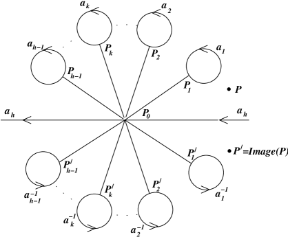
Figure 6: $\Sigma_{(0,h)}$ is represented in the upper half-plane with $h$ boundaries, $\bf{a}_{h}$ being the real axis and the remaining $\bf{a}_{1},\dots,\bf{a}_{h-1}$ being the boundaries of $h{-}1$ holes cut out. The double cover is obtained by including the lower half-plane with the $\mathbb{Z}_{2}$ involution $z\to\bar{z}$. The images of boundaries $\bf{a}_{1},\dots,\bf{a}_{h-1}$ are shown as $\bf{a}_{1}^{-1},\dots,\bf{a}_{h-1}^{-1}$ while $\bf{a}_{h}$ is fixed. $\bf{a}_{k}$ and $\bf{a}^{-1}_{k}$, for each $k=1,\dots,h{-}1$, are glued together to yield a genus $h{-}1$ surface. Simply-connected surface is obtained by cutting lines $P_{0}$ to $P_{k}$ and $P_{0}$ to $P_{k}^{\prime}$ for each $k$. ${\bf b}_{k}$ cycle is defined as the path from $P_{0}$ to $P_{k}$ which is identified with $P_{k}^{\prime}$, and then from $P_{k}^{\prime}$ to $P_{0}$, (in a different sheet due to the twist along $\bf b_{k}$ cycles).

One gets the genus $h-1$ surface by gluing ${\bf a}_{i}$ and ${\bf a}_{i}^{-1}$ cycles together. The real axis is the boundary ${\bf a}_{h}$ which sits on the $h$-th brane while the remaining ${\bf a}_{i}$ cycles sit on the $i$-th brane. The $\mathbb{Z}_{2}$ involution takes the upper half-plane to the lower half-plane. Let

$$A_{jk}=\int_{{\bf a}_{k}}\omega_{j,\{g\}}~{}~{}~{},~{}~{}~{}B_{jk}=\int_{{\bf b}_{k}}\omega_{j,\{g\}}\,.$$ (A.7)

Here the ${\bf b}_{k}$ cycle is defined as follows. If $P_{k}$ is a point on the ${\bf a}_{k}$ cycle and $P_{k}^{\prime}$ is its $\mathbb{Z}_{2}$ image on the ${\bf a}_{k}^{-1}$ cycle, then the ${\bf b}_{k}$ cycle is the line from $P_{0}$ to $P_{k}$ which is identified with $P_{k}^{\prime}$ (on a different sheet due to $g_{k}$ twist) via gluing and then from $P_{k}^{\prime}$ to $P_{0}$ in this different sheet. Note that ${\bf b}_{k}$ is not a closed contour when $g_{k}$ is non-trivial. As a result, the integrals of closed twisted differentials will depend on the choice of the base point $P_{0}$. Let $b_{jk}=\int_{P_{0}}^{P_{k}}\omega_{j,\{g\}}$ on the path indicated in the Fig. 6, then

$$B_{jk}=b_{jk}-g_{k}\bar{b}_{jk}\,.$$ (A.8)

In particular, this implies that $g_{k}^{-\frac{1}{2}}B_{jk}$ is purely imaginary. As noted above, when $g_{k}$ is non-trivial, $B_{jk}$ depends on the choice of the base point $P_{0}$.

Integrating around trivial cycle $\prod_{i=1}^{h-1}({\bf a}_{i}{\bf b}_{i}{\bf a}_{i}^{-1}{\bf b}_{i}^{-1})$ gives the condition

$$\sum_{i=k}^{h-1}(1-g_{k}^{-1})A_{jk}=0\,.$$ (A.9)

Since at least one of the $g_{i}$ is not identity (say $g_{h-1}$), we can always eliminate one of the $A_{jk}$’s (say $A_{j(h-1)}$). We can furthermore normalize $\omega_{j,\{g\}}$ so that

$$A_{jk}=g_{j}^{\frac{1}{2}}\delta_{jk}~{}~{}~{},~{}~{}~{}{\rm for}~{}~{}~{}k=1,...,h-2.$$ (A.10)

Then the above equation implies

$$A_{j(h-1)}=-g_{h-1}^{\frac{1}{2}}\frac{\sin(\theta_{j})}{\sin(\theta_{h-1})}.$$ (A.11)

We will also need the holomorphic differentials $\omega_{j\{g^{-1}\}}$ that are twisted oppositely to $\omega_{j\{g\}}$. We will denote the corresponding periods by $A^{\prime}_{jk}$ and $B^{\prime}_{jk}$ and $b^{\prime}_{jk}$. They satisfy all the above equations with $g_{k}$ replaced by $g_{k}^{-1}$.

Given any two closed twisted differentials $\rho$ and $\rho^{\prime}$ that are twisted by $\{g\}$ and $\{g^{-1}\}$ respectively, one can evaluate, by using the standard methods for the marking shown in Fig. 6, the following integral:

$$\int_{\Sigma}\rho\wedge\rho^{\prime}=\sum_{k=1}^{h-1}[B_{k}A^{\prime}_{k}-A_{k}B^{\prime}_{k}+\sum_{\ell=1}^{k}(1-g_{k}g_{\ell}^{-1})A_{\ell}A^{\prime}_{k}]\,,$$ (A.12)

where $A_{k}=\int_{{\bf a}_{k}}\rho$, $A^{\prime}_{k}=\int_{{\bf a}_{k}}\rho^{\prime}$, $B_{k}=\int_{{\bf b}_{k}}\rho$ and $B^{\prime}_{k}=\int_{{\bf b}_{k}}\rho^{\prime}$.

The $(1,1)$ forms $\omega_{j,\{g\}}\wedge\bar{\omega}_{k,\{g\}}$ are untwisted and therefore can be integrated on the Riemann surface. Using (A.12) and the periods (A.8), (A.10) and (A.11), we find

$$\int_{\Sigma}\omega_{j,\{g\}}\wedge\bar{\omega}_{k,\{g\}}=\tau_{jk}-\bar{\tau}_{kj}\,,$$ (A.13)

where

$$\tau_{jk}=D_{jk}-C_{jk}$$ (A.14)

and $C$ is a purely imaginary symmetric $(h-2)\times(h-2)$ matrix which does not depend on the world-sheet moduli. It is given by

$$C_{jk}=-i\frac{\sin(\theta_{k})\sin(\theta_{j}-\theta_{h-1})}{\sin(\theta_{h-1})}~{}~{}~{},~{}~{}~{}~{}~{}{\rm{for}}~{}~{}~{}j\geq k.$$ (A.15)

On the other hand, the matrix $D$ depends on the world-sheet moduli and is given in terms of the periods $B_{jk}$ as follows:

$$D_{jk} = \frac{g_{k}^{-\frac{1}{2}}}{2i\sin(\theta_{h-1})}\int_{b_{k}b_{h-1}b_{k}^{-1}b_{h-1}^{-1}}\omega_{j,\{g\}}$$ (A.16)

$$= g_{k}^{-\frac{1}{2}}B_{jk}-\frac{\sin(\theta_{k})}{\sin(\theta_{h-1})}g_{h-1}^{-\frac{1}{2}}B_{j(h-1)}\,.$$

It is important to note that while $B_{jk}$ depends on the base point $P_{0}$, $D_{jk}$ does not. This is due to the fact that the cycle ${\bf b}_{k}{\bf b}_{h-1}{\bf b}_{k}^{-1}{\bf b}_{h-1}^{-1}$ is a closed contour even when $g_{k}$ is non-trivial. Due to Eq.(A.8), $D$ is also purely imaginary, however it is in general not symmetric. As a consequence the right hand side of equation (A.13) is purely imaginary and

$$\tau_{jk}-\bar{\tau}_{kj}=2(\tau^{S})_{jk},$$ (A.17)

where $\tau^{S}$ is the symmetric part of $\tau$.

Similarly, we can define the corresponding quantities for oppositely twisted differentials and the corresponding periods $\tau^{\prime}_{jk}$ satisfy the same equations with $g_{k}$ replaced by $g_{k}^{-1}$. Finally, we have the relation

$$0=\int_{\Sigma}\omega_{j,\{g\}}\wedge\omega_{k,\{g^{-1}\}}=\tau_{jk}-\tau^{\prime}_{kj}.$$ (A.18)

In the untwisted case, a similar equation implies that the period matrix is symmetric, however in the twisted case it only says that the transposed $\tau$ is equal to $\tau^{\prime}$.

Using the twisted differentials, one can write the classical solution for $Z$ as

$$dZ=\sum_{j=1}^{h-2}[L_{j}\omega_{j,\{g\}}+\tilde{L}_{j}\bar{\omega}_{j,\{g^{-1}\}}].$$ (A.19)

Integrals around ${\bf a}_{k}$ cycles should give the windings $n_{k}v_{k}$, which implies that $\int_{a_{k}}dZ=n_{k}v_{k}$. Furthermore, $\int_{P_{0}}^{P_{k}}dZ=(m_{k}+y_{k})w_{k}$, due to the boundary conditions (A.1). This implies

$$\int_{{\bf b}_{k}}dZ=(m_{k}+y_{k})(w_{k}-g_{k}\bar{w}_{k})=2i(m_{k}+y_{k})g_{k}^{\frac{1}{2}}\frac{T_{2}}{|v_{k}|}\,,$$ (A.20)

where in the second equality we used the fact that $w_{k}.*v_{k}=T_{2}$. Here, $y_{k}$ are shifted by $y_{h}\frac{w_{h}.*v_{i}}{T_{2}}$, due to the fact that we are choosing our coordinates so that the $h$-th brane lies on the real axis. We can then solve for $L$ and $\tilde{L}$ as

$$L = \frac{N}{2}+\frac{1}{2\tau^{S}}[(\tau^{A}+C)N+2M]$$ (A.21)

$$\tilde{L} = \frac{N}{2}-\frac{1}{2\tau^{S}}[(\tau^{A}+C)N+2M],$$ (A.22)

where $\tau^{S}$ and $\tau^{A}$ are the symmetric and anti-symmetric parts of $\tau$, respectively, and $L$, $\tilde{L}$, $N$ and $M$ are $(h-2)$-dimensional column vectors whose components are respectively $L_{j}$, $\tilde{L}_{j}$, $N_{j}=n_{j}|v_{j}|$ while $M_{j}$ is given by

$$M_{j}=i\frac{T_{2}}{|v_{j}|}[(m_{j}+y_{j})-\frac{v_{h}.*v_{j}}{v_{h}.*v_{h-1}}(m_{h-1}+y_{h-1})].$$ (A.23)

The classical action is

$$S = -i\pi(L^{T}\tau^{S}L+\tilde{L}^{T}\tau^{S}\tilde{L})+2\pi i\sum_{j=1}^{h-2}n_{j}W_{j}$$ (A.24)

$$= i\pi[N^{T}\tau^{S}N+\{2M+(\tau^{A}+C)N\}^{T}(\tau^{S})^{-1}\{2M+(\tau^{A}+C)N\}]$$

$$+~{}2\pi i\sum_{j=1}^{h-2}n_{j}W_{j},$$

where $W_{j}$ is the Wilson line on the world-volume of the $j$-th brane.

Poisson resummation over $m_{j}$ for $j=1,\dots,h-2$ gives rise to the following instanton contribution

$$Z_{\rm{inst}} = [\,\prod_{j=1}^{h-2}\frac{|v_{j}|}{T_{2}}\,]({\rm{det}}\tau^{S})^{\frac{1}{2}}\sum_{n_{j},k_{j},m_{h-1}}e^{i\pi(N^{T}\tau^{S}N+\frac{1}{4}K^{T}\tau^{S}K)-\pi K^{T}\tau^{A}N}$$ (A.25)

$$\times~{}e^{2\pi i\sum_{j=1}^{h-2}(k_{j}{\tilde{y}}_{j}+n_{j}W_{j})}\,e^{2\pi i\sum_{j=1}^{h-2}k_{j}\frac{v_{h}.*v_{j}}{v_{h}.*v_{h-1}}m_{h-1}}e^{-\pi K^{T}CN},$$

where $K$ is a column vector with components $K_{j}=\frac{|v_{j}|}{T_{2}}k_{j}$ and ${\tilde{y}}_{j}$ is the effective Wilson line (A.3) in the Dirichlet direction. The sum over $n_{j}$ ($j=1,\dots,h-2$) is over integers that satisfy the constraint (A.4) while the sum over $k_{j}$ ($j=1,\dots,h-2$) is over all integers. Finally, the sum over $m_{h-1}$ ranges from $0$ to $p-1$, where $p$ is the smallest integer such that $p\frac{v_{h}.*v_{j}}{v_{h}.*v_{h-1}}$ is integer for all $j$. The latter sum reduces the $k_{j}$ sums to a sublattice satisfying the constraint

$$\sum_{j=1}^{h-2}k_{j}\frac{v_{h}.*v_{j}}{v_{h}.*v_{h-1}}={\rm integer}.$$ (A.26)

This constraint is exactly as the one for the $n_{j}$ and from the above discussion it follows that this implies that there exist integers $k_{a}$, $a=1,\dots,h$, such that $\sum_{a}k_{a}v_{a}=0$. In fact, $K_{a}=k_{a}*v_{a}/T_{2}$ is a vector in the dual lattice and describes the momentum in the Dirichlet direction for the ${a}$-th brane (i.e. in the direction perpendicular to $v_{a}$).

The phase $e^{-\pi K^{T}CN}$ is independent of the world-sheet moduli and of the target space moduli. One can show using the constraints (A.4) and the similar one for $k_{j}$, that $iK^{T}CN$ is an integer implying that this phase is $\pm 1$.

We can also include a $B$ field on the plane. The contribution of the $B$ field to the instanton action is

$$S_{B}=\frac{2\pi B}{T_{2}}N^{T}(M+\frac{1}{2}CN).$$ (A.27)

Including this contribution (after the Poisson resummation) in Eq.(A.25), one finally obtains

$$Z_{\rm{inst}} = p\,[\,\prod_{j=1}^{h-2}\frac{|v_{j}|}{T_{2}}\,]({\rm{det}}\tilde{\tau}^{S})^{\frac{1}{2}}\sum_{n_{j},k_{j}}e^{\frac{i\pi}{T_{2}}(n^{T}\bar{T}+\frac{1}{2}k^{T})\tilde{\tau}(nT+\frac{1}{2}k)}$$ (A.28)

$$\times~{}e^{2\pi i(k_{j}{\tilde{y}}_{j}+n_{j}W_{j})}\,e^{-\pi K^{T}CN},$$

where $n$ and $k$ are $(h-2)$-dimensional column vectors with integer entries $n_{j}$ and $k_{j}$ satisfying the constraints (A.4) and (A.26), respectively, and

$$\tilde{\tau}_{jk}\equiv\frac{|v_{j}||v_{k}|}{T_{2}}\tau_{jk}.$$ (A.29)

It is worth noting that $\tau_{jk}$ depend only on the world-sheet moduli and the twist angles. In turn, these angles depend on the target space modulus $U$, but not on $T$. Since $\frac{|v_{j}||v_{k}|}{T_{2}}$ does not depend on $T$ as well, it follows that ${\tilde{\tau}}$ also only depends on $U$, but not on $T$. Thus the $T$-dependence of the partition function is explicit in (A.28). The $U$ dependence, however, is implicit and appears through ${\tilde{\tau}}$.

Let us now consider the degeneration limit of $\tau$ when ${\bf a}_{1}$ cycle vanishes. In Fig. 6, this amounts to shrinking ${\bf a}_{1}$ and ${\bf a}_{1}^{-1}$ cycles to points $z_{1}$ and its image, respectively. In this limit, the usual period matrix $t$ given by the untwisted differentials degenerates as $t_{11}\rightarrow i\infty$. Since the twisted $\omega_{1}$ will degenerate to a twisted differential with two simple poles at $z_{1}$ and its image, with residues $g_{1}^{\frac{1}{2}}$ and $-g_{1}^{-\frac{1}{2}}$, respectively. Then Eqs. (A.14), (A.15), (A.16) and (A.8) imply that $\tau_{11}\rightarrow t_{11}$ modulo finite terms. Thus the $t_{11}$ dependence of the partition function is

$$q_{1}^{\frac{1}{2}[n_{1}\vec{v}_{1}+(k_{1}+Bn_{1})\frac{*\vec{v}_{1}}{T_{2}}]^{2}}~{}~{}~{},~{}~{}~{}~{}q_{1}=e^{2i\pi t_{11}}.$$ (A.30)

This agrees with the fact that the boundary state describing the brane parallel to the vector $\vec{v}_{1}$ involves precisely the lattice states $[n_{1}\vec{v}_{1}+(k_{1}+Bn_{1})\frac{*\vec{v}_{1}}{T_{2}}]$. As a further check, one might ask what happens when we take the limit of shrinking the ${\bf a}_{h-1}$ cycle to a point $z_{h-1}$. Since in our treatment the $(h-1)$-th boundary played a special role, it is not immediately obvious that the corresponding degeneration would have a correct interpretation in terms of the boundary state. In this limit all the basis elements of twisted differentials $\omega_{j,\{g\}}$ develop simple poles at $z_{h-1}$ and its image, with residues $-\frac{\sin(\theta_{j})}{\sin(\theta_{h-1})}g_{h-1}^{\pm\frac{1}{2}}$, respectively. Then Eqs. (A.14), (A.15), (A.16) and (A.8) imply that the leading behavior of the twisted period matrix is given by

$$\tau_{jk}\rightarrow\frac{\sin(\theta_{j})\sin(\theta_{k})}{\sin(\theta_{h-1})^{2}}t_{(h-1)(h-1)}$$ (A.31)

and the $q_{h-1}\equiv t_{(h-1)(h-1)}$ dependence of the partition function is

$$q_{h-1}^{\frac{1}{2}\sum_{j,k=1}^{h-2}\frac{\sin(\theta_{j})\sin(\theta_{k})}{\sin(\theta_{h-1})^{2}}\frac{|v_{j}||v_{k}|}{T_{2}^{2}}(n_{j}T+k_{j})(n_{k}\bar{T}+k_{k})}$$ (A.32)

$$=q_{h-1}^{\frac{1}{2}[n_{h-1}\vec{v}_{h-1}+(k_{h-1}+Bn_{h-1})\frac{*\vec{v}_{h-1}}{T_{2}}]^{2}},$$ (A.33)

where we used the constraints (A.4) and (A.26) for $n_{j}$ and $k_{j}$. This again agrees with the boundary state of the $(h-1)$-th brane.

Finally, let us consider the case when all the $h-1$ ${\bf a}_{j}$-cycles are shrunk to points $z_{j}$ for $j=1,\dots,h-1$. Then the partition function must describe a $(h-1)$-point function on the disk whose boundary sits on the $h$-th brane. The vertices at the $h-1$ points are boundary states on the $j$-th brane, namely

$$V(z_{j},n_{j},k_{j})=e^{in_{j}\vec{v}_{j}.(\vec{X}_{L}-\vec{X}_{R})+\frac{i}{T_{2}}(k_{j}+Bn_{j})*\vec{v}_{j}.(\vec{X}_{L}+\vec{X}_{R})}(z_{j})$$ (A.34)

for integers $n_{j}$ and $k_{j}$ satisfying the constraints (A.4), (A.26). To see this, we note that, in this limit, $\omega_{i}$ become

$$\omega_{i}(z)=\frac{1}{2\pi i}[\frac{e^{i\theta_{i}}}{z-z_{i}}-\frac{e^{-i\theta_{i}}}{z-\bar{z}_{i}}-\frac{\sin(\theta_{i})}{\sin(\theta_{h-1})}(\frac{e^{i\theta_{h-1}}}{z-z_{h-1}}-\frac{e^{-i\theta_{h-1}}}{z-\bar{z}_{h-1}})]\,.$$ (A.35)

Using this we can compute $\tau$ and, after some algebra and taking care of the logarithmic branch cuts, we indeed find that the result is

$$\sum_{n_{j},k_{j}}\langle\prod_{j=1}^{h-1}q_{j}^{\Delta(n_{j},k_{j})}V(z_{j},n_{j},k_{j})\rangle\,.$$ (A.36)

So far, we have discussed the contribution of the classical solutions to the partition function. In the topological amplitude discussed in this paper we actually need the correlation function

$$\langle\prod_{j=1}^{h-2}[\bar{\psi}\partial Z(w_{j})+\bar{\psi}\partial Z(w^{\prime}_{j})]\rangle_{h},$$ (A.37)

where $w^{\prime}_{j}$ is the image of $w_{j}$. In the topological theory ${\bar{\psi}}$ are dimension one fields and have $h-2$ zero modes and therefore are replaced by the $h-2$ twisted differentials $\omega_{i}$. Similarly plugging in the classical solution for $\partial Z$ (A.19), (A.22) and doing the Poisson resummation over the integers $m_{j}$, we find that the world-sheet supercurrents in the correlation function are replaced by $\det(\Omega_{i}(w_{j}))$, where

$$\Omega_{i}=\sum_{j=1}^{h-2}\frac{1}{T_{2}}(n_{j}T+k_{j})v_{j}(\omega_{j,{g}}\omega_{i,{g^{-1}}}+{\rm c.c.}).$$ (A.38)

The above discussion has been limited to the case of magnetized D9 branes on $T^{6}$, and as a result the boundaries (${\bf a}$-cycles) are untwisted. This allowed us to normalize the Prym differentials along the ${\bf a}_{i}$-cycles for $i=1,\dots,h-2$. One can generalize the above to the case of orbifolds or fractional branes where some (or all) of the a-cycles are also twisted. The twisted ${\bf a}_{i}$ cycles are now not closed, however, we can choose instead the closed cycles ${\bf a}_{i}{\bf b}_{i}{\bf a}_{i}^{-1}{\bf b}_{i}^{-1}$ to normalize the Prym differentials. This analysis has been carried out in Ref.[11] in the context of closed strings. It is straightforward, to generalize the method of this reference to the case of open strings.

References

- [1] M. Bershadsky, S. Cecotti, H. Ooguri and C. Vafa, Nucl. Phys. B 405 (1993) 279 [arXiv:hep-th/9302103] and Commun. Math. Phys. 165 (1994) 311 [arXiv:hep-th/9309140].
- [2] I. Antoniadis, E. Gava, K.S. Narain and T.R. Taylor, Nucl. Phys. B 413 (1994) 162 [arXiv:hep-th/9307158].
- [3] H. Ooguri and C. Vafa, Adv. Theor. Math. Phys. 7 (2004) 405 [arXiv:hep-th/0303063] and Adv. Theor. Math. Phys. 7 (2003) 53 [arXiv:hep-th/0302109].
- [4] N. Berkovits, H. Ooguri and C. Vafa, Commun. Math. Phys. 252 (2004) 259 [arXiv:hep-th/0310118].
- [5] I. Antoniadis, E. Gava, K. S. Narain and T. R. Taylor, Nucl. Phys. B 476 (1996) 133 [arXiv:hep-th/9604077].
- [6] J. Polchinski and E. Witten, Nucl. Phys. B 460, 525 (1996) [arXiv:hep-th/9510169].
- [7] C. Bachas, arXiv:hep-th/9503030; M. Berkooz, M. R. Douglas and R. G. Leigh, Nucl. Phys. B 480, 265 (1996) [arXiv:hep-th/9606139].
- [8] I. Antoniadis and T. R. Taylor, Nucl. Phys. B 695 (2004) 103 [arXiv:hep-th/0403293].
- [9] S. K. Blau, S. Carlip, M. Clements, S. Della Pietra and V. Della Pietra, Nucl. Phys. B 301 (1988) 285; M. Bianchi and A. Sagnotti, Phys. Lett. B 211 (1988) 407.
- [10] M. Bianchi and A. Sagnotti, Phys. Lett. B 231 (1989) 389.
- [11] K. S. Narain, M. H. Sarmadi and C. Vafa, Nucl. Phys. B 356 (1991) 163.
- [12] I. Antoniadis, H. Partouche and T. R. Taylor, Nucl. Phys. B 499, 29 (1997) [arXiv:hep-th/9703076]; D. Lüst and S. Stieberger, arXiv:hep-th/0302221.
- [13] N. Arkani-Hamed and S. Dimopoulos, arXiv:hep-th/0405159; G. F. Giudice and A. Romanino, Nucl. Phys. B 699, 65 (2004) [Erratum-ibid. B 706, 65 (2005)] [arXiv:hep-ph/0406088]; I. Antoniadis and S. Dimopoulos, Nucl. Phys. B 715, 120 (2005) [arXiv:hep-th/0411032].
- [14] I. Antoniadis, Phys. Lett. B 246 (1990) 377; J. D. Lykken, Phys. Rev. D 54 (1996) 3693 [arXiv:hep-th/9603133]; I. Antoniadis, N. Arkani-Hamed, S. Dimopoulos and G. R. Dvali, Phys. Lett. B 436 (1998) 257 [arXiv:hep-ph/9804398].
- [15] I. Antoniadis, E. Dudas and A. Sagnotti, Phys. Lett. B464 (1999) 38 [arXiv:hep-th/9908023]; G. Aldazabal and A. M. Uranga, JHEP 9910 (1999) 024 [arXiv:hep-th/9908072].