YITP 05-35
CERN-TH-PH/2005-128
hep-th/0507173
Moduli Stabilisation in Heterotic String Compactifications

In this paper we analyze the structure of supersymmetric vacua in compactifications of the heterotic string on certain manifolds with SU(3) structure. We first study the effective theories obtained from compactifications on half-flat manifolds and show that solutions which stabilise the moduli at acceptable values are hard to find. We then derive the effective theories associated with compactification on generalised half-flat manifolds. It is shown that these effective theories are consistent with four-dimensional $N=1$ supergravity and that the superpotential can be obtained by a Gukov-Vafa-Witten type formula. Within these generalised models, we find consistent supersymmetric (AdS) vacua at weak gauge coupling, provided we allow for general internal gauge bundles. In simple cases we perform a counting of such vacua and find that a fraction of about $1/1000$ leads to a gauge coupling consistent with gauge unification.

1 Introduction

There is now a considerable body of work on moduli stabilization, facilitated by flux of the Neveu Schwarz-Neveu Schwarz (NSNS) and Ramond-Ramond (RR) anti-symmetric tensor fields, in the context of type II theories. Specifically, within type IIB it has been shown [1] that a combination of NSNS and RR three-form flux can stabilize the dilaton and all complex structure moduli, while the Kähler moduli have to be fixed by other effects such as non-perturbative contributions [2] or perhaps higher-order $\alpha^{\prime}$ corrections [3]. The consistency of these procedures, including the interplay between $\alpha^{\prime}$ and non-perturbative corrections, was analysed in Refs [4, 5, 6, 7, 8, 9, 10] Within type IIA theories, on the other hand, both odd and even degree form field strengths are available, so that flux potentials for complex structure moduli as well as Kähler moduli will typically be generated [11, 12] (see also Ref. [13] for $N=1$ models). One may therefore hope that all moduli can be stabilised by flux in some such models and specific examples have indeed been found [14, 15, 16, 17, 18], although it appears that in generic models of this kind some flat directions are still left over.

Traditionally, the heterotic string has been considered the most attractive string theory, with the presence of (preferably $E_{8}\times E_{8}$) ten-dimensional gauge fields leading to a large number of supersymmetric compactifications with phenomenologically interesting properties [19]. It has also been known for a long time that heterotic NSNS three-form flux can stabilize all complex structure moduli of the theory [20, 21]. More recently, this subject was addressed in Refs [22, 23]. However, in the absence of any further (RR) antisymmetric tensor fields, the potential for stabilizing the remaining moduli seems rather limited compared to type II theories. This apparent problem can be overcome by departing from Calabi-Yau compactifications and by considering the heterotic string on general manifolds with SU(3) structure. Such models were analysed in Refs [24, 25, 26, 27, 28, 29, 30] where general aspects of compactifications on non-Kähler manifolds were studied. Recently, a more general analysis which takes into account the effects of a gaugino condensate in ten dimensions appeared in Ref. [31]. The generic form of the superpotential was inferred in [25, 26, 27], but its detailed analysis was not possible due to the lack of knowledge of the moduli space of these manifolds. On the other hand the low energy effective action and an explicit form for the superpotential in terms of the low energy fields were found in Ref. [32], where half-flat mirror manifolds were used as compactification spaces. Such manifolds arise in the context of type II mirror symmetry with NS fluxes [33] and, in some appropriate region, their moduli space was conjectured to be similar to that of a normal Calabi–Yau manifold. This conjecture has been applied in Ref. [32] to derive the low-energy theory for these compactifications and, in particular, the superpotential as an explicit function of the moduli fields. In particular, it was found that the intrinsic torsion of the half-flat mirror manifolds gives rise to a superpotential for the Kähler moduli. These results suggest that, by combining the intrinsic torsion of sufficiently general classes of $\mbox{SU}(3)$ structure manifolds with NSNS flux, moduli stabilization in heterotic compactifications can be as flexible as in type II models.

This is precisely the line of work we would like to further develop in the present paper. We will first study in detail supersymmetric moduli stabilization in the heterotic string on half-flat mirror manifolds, based on the effective theories of Ref. [32]. As we will see, the torsion of half-flat manifolds and the allowed $H$-fluxes are insufficient to fix all Kähler and complex structure moduli. We therefore move on to the more general class of manifolds with $\mbox{SU}(3)$ structure described in Refs [34, 35, 36], which we will refer to as generalised half-flat manifolds. For this class of spaces we first show, by an explicit reduction of the bosonic action, that the heterotic Gukov-Vafa-Witten type formula for heterotic compactifications [32, 37, 38] leads to the correct result for the superpotential. This result is then applied to a detailed analysis of moduli stabilization for those models.

The flux and torsion superpotential, ${\cal W}$, for all models considered in this paper is a function of the Kähler moduli $T^{i}$ and complex structure moduli $Z^{a}$, but it turns out to be independent of the dilaton $S$. Hence, the dilaton is not stabilised at this stage. However, in the $E_{8}\times E_{8}$ case, one expects hidden sector gaugino condensation to generate a non-perturbative dilaton superpotential which should be added to ${\cal W}$. We will, therefore, use this non-perturbative contribution to stabilize the dilaton. It turns out that, in order to fix $S$ at sufficiently weak coupling (and to be in the large radius and large complex structure limits) we need global minima for the Kähler and complex structure moduli which correspond to superpotential values ${\cal W}_{0}$ with $|{\cal W}_{0}|\ll 1$. This is quite analogous to a similar requirement in type IIB models [2], where it is necessary to ensure moduli stabilization at large radius. The original models of heterotic gaugino condensation with flux [20, 21] were discarded precisely because this condition was difficult to satisfy due to the quantization of fluxes. However, we find that cancellations leading to small $|{\cal W}_{0}|$ are possible for our generalised models. We carry out a statistical analysis in those cases, counting the number of vacua as a function of $|{\cal W}_{0}|$ and the maximal flux value. As the value of $|{\cal W}_{0}|$ determines the value of the dilaton, this counting analysis is directly relevant to the question of how many vacua realize a phenomenologically acceptable gauge coupling.

The outline of the paper is as follows. In Section 2 we briefly review the low energy effective theory of the heterotic string on half-flat mirror manifolds [32]. In addition, we work out the generalization of this effective theory expected for the more general spaces proposed in [34]. We will show explicitly that the potential obtained from compactification (which includes a part from the non-vanishing scalar curvature of the internal space) can be obtained from a Gukov-Vafa-Witten type superpotential for manifolds with SU(3) structure, which was derived in [32]. In Section 3 we set up our four-dimensional models in a way suitable for the discussion of moduli stabilization which includes gaugino condensation and flux quantization. This section is largely self-contained and the reader mostly interested in the four-dimensional aspects of our analysis may want to skip Section 2 and move on to Section 3 straight away. Moduli stabilization within models based on half-flat mirror manifolds [32] is discussed in Section 4. In Section 5 we discuss the models based on the more general half-flat spaces introduced in Section 2. We conclude in Section 6. Various technical details are deferred to the three appendices. Appendix A contains a calculation of the scalar curvature of the generalised half-flat spaces, which is essential in establishing the consistency of the generalised models of Section 2. In Appendix B we have collected a number of useful relations on special geometry, while Appendix C summarizes our four-dimensional $N=1$ supergravity conventions. It also includes an elementary proof that supersymmetric AdS vacua of this theory are always stable.

2 The heterotic string on half-flat manifolds

In this section we will review the compactification of the heterotic string on half-flat mirror manifolds [32] and present an extension of this work to the spaces proposed in Ref. [34, 35, 36].

2.1 The heterotic string on half-flat mirror manifolds

Half-flat mirror manifolds arise in the context of type II mirror symmetry [33] and can be thought of as mirror duals to Calabi-Yau manifolds with NSNS flux. More specifically, given a mirror pair $(X,Y)$ of Calabi-Yau manifolds, the mirror of, say, IIB on $Y$ in the presence of NSNS flux is IIA on a half-flat mirror manifold $\hat{X}$ (without flux). This half-flat mirror manifold $\hat{X}$ is closely related to the original Calabi-Yau mirror $X$ in that it can be characterized by the two Hodge numbers $h^{(1,1)}$ and $h^{(2,1)}$ of $X$ and carries sets of two- three- and four-forms analogous to the sets of harmonic forms on the Calabi-Yau space $X$. Specifically, on $\hat{X}$ we denote by $(\omega_{i})$ and $(\tilde{\omega}^{j})$ a basis for the two- and four-forms respectively, where $i,j,\dots=1,\dots,h^{(1,1)}$, which satisfy

$$\int_{\hat{X}}\omega_{i}\wedge\tilde{\omega}^{j}=\delta_{i}^{j}\;.$$ (2.1)

Further, on $\hat{X}$, one can define a set of symplectic three forms $(\alpha_{A},\beta^{B})$ where $A,B,\dots=0,\dots,h^{(2,1)}$ with

$$\int_{X}\alpha_{A}\wedge\beta^{B}=\delta_{A}^{B}\;,\quad\int_{X}\alpha_{A}\wedge\alpha_{B}=\int_{X}\beta^{A}\wedge\beta^{B}=0\;.$$ (2.2)

Being manifolds with $\mbox{SU}(3)$ structure [39], half-flat mirror manifolds carry a two-form $J$ and three-form $\Omega$ which are the analog of the Kähler form and the holomorphic $(3,0)$ form on Calabi-Yau manifolds . As on Calabi-Yau manifolds these forms can be expanded as

$$J = t^{i}\omega_{i}\;,$$ (2.3)

$$\Omega = {\cal Z}^{A}\alpha_{a}-{\cal G}_{A}\beta^{A}\;,$$ (2.4)

where $t^{i}$ and ${\cal Z}^{A}$ are the equivalent of Kähler and complex structure moduli. As usual, the coefficient ${\cal G}_{A}$ can be obtained from a holomorphic pre-potential ${\cal G}={\cal G}({\cal Z}^{A})$, homogeneous of degree two, as

$${\cal G}_{A}=\frac{\partial{\cal G}}{\partial{\cal Z}^{A}}\;.$$ (2.5)

So far, the set-up has been exactly as for Calabi-Yau manifolds. The main difference is that the forms $(\omega_{i})$ and $(\alpha_{A},\beta^{A})$ are no longer harmonic but rather satisfy

$$d\omega_{i}=e_{i}\beta^{0}\;,\quad d\alpha_{0}=e_{i}\tilde{\omega}^{i}\;,\quad d\alpha_{a}=d\beta^{A}=0\;,\ \quad d\tilde{\omega}^{i}=0\;.$$ (2.6)

Here $e_{i}$ are $h^{(1,1)}$ parameters (real numbers) which characterize the torsion of the half-flat mirror manifold under consideration.

Having described the basic structure of half-flat mirror manifolds, let us now review the compactification of the heterotic string (at lowest order in $\alpha^{\prime}$) on those spaces. Besides the metric, there are two other bosonic fields, namely the dilaton $s=\exp(-2\phi)$ and the NSNS two-form $\hat{B}$. The latter can be expanded as

$$\hat{B}=B+\tau^{i}\omega_{i}\;,$$ (2.7)

where $B$ is a four-dimensional two-form which can be dualised to a scalar $\sigma$ and $\tau^{i}$ is a set of axions. Together with the dilaton and the Kähler moduli, these fields pair up into four-dimensional chiral multiplets as

$$T^{i} = \tau^{i}+it^{i}\;,$$ (2.8)

$$S = \sigma+is\;.$$ (2.9)

In terms of the projective coordinates ${\cal Z}^{A}$ the complex structure chiral multiplets $Z^{a}$, where $a,b,\dots=1,\dots,h^{(2,1)}$, are obtained by $Z^{a}={\cal Z}^{a}/{\cal Z}^{0}$ and we write these fields as

$$Z^{a}=\zeta^{a}+iz^{a}\;.$$ (2.10)

The Kähler potential for those fields in the large radius limit is then of the standard Calabi-Yau form, that is,

$$K=K^{(T)}+K^{(Z)}+K^{(S)}\;,$$ (2.11)

with

$$K^{(T)} = -\ln\left(\frac{4}{3}\mathcal{K}\right)\;,$$

$$K^{(Z)} = -\ln\left(\frac{4}{3}\tilde{\mathcal{K}}\right)\;,$$ (2.12)

$$K^{(S)} = -\ln\left(i(\bar{S}-S)\right)\;,$$

and

$$\mathcal{K} = \frac{i}{8}d_{ijk}(T^{i}-\bar{T}^{i})(T^{j}-\bar{T}^{j})(T^{k}-\bar{T}^{k})=d_{ijk}t^{i}t^{j}t^{k}\;,$$ (2.13)

$$\tilde{\mathcal{K}} = \frac{3i}{4}\left(\bar{\cal Z}^{A}{\cal G}_{A}-{\cal Z}^{A}\bar{\cal G}_{A}\right)\;.$$ (2.14)

Here, $d_{ijk}$ are numbers analogous to the intersection numbers of the associated Calabi-Yau space $X$. Later, we will be working in the large complex structure limit, where the pre-potential $\mathcal{G}$ can be written as

$${\cal G}=-\frac{1}{6}\frac{\tilde{d}_{abc}{\cal Z}^{a}{\cal Z}^{b}{\cal Z}^{c}}{{\cal Z}^{0}}\;,$$ (2.15)

with $\tilde{d}_{abc}$ analogous to the intersection of the associated mirror Calabi-Yau space $Y$. In this case, the complex structure Kähler potential takes a form similar to the one for the Kähler moduli, that is

$$\tilde{\mathcal{K}}=\frac{i}{8}\tilde{d}_{abc}(Z^{a}-\bar{Z}^{a})(Z^{b}-\bar{Z}^{b})(Z^{c}-\bar{Z}^{c})=\tilde{d}_{abc}z^{a}z^{b}z^{c}\;.$$ (2.16)

Let us now discuss the superpotential. In Ref. [32] it has been shown that, for general heterotic compactifications on manifolds with $\mbox{SU}(3)$ structure, the superpotential to order ${\alpha^{\prime}}$ can be obtained from the Gukov-Vafa-Witten type formula

$$W=\sqrt{8}\int_{\hat{X}}\Omega\wedge(\hat{H}+idJ)\;,$$ (2.17)

where $\hat{H}$ is the NSNS field strength. For half-flat mirror manifolds this field strength can be written as

$$\hat{H}=dB+d\tau^{i}\wedge\omega_{i}+\tau^{i}e_{i}\beta^{0}+H_{\rm flux}\;.$$ (2.18)

where the first three terms have been computed by taking the exterior derivative of Eq. (2.7). Note that the third term is new and arises because the forms $\omega_{i}$ are no longer closed, see Eq. (2.6). We have also added on an additional NSNS flux contribution

$$H_{\rm flux}=(\mu^{a}\alpha_{a}-\epsilon_{a}\beta^{a})\;,$$ (2.19)

with electric and magnetic flux parameters $\epsilon_{a}$ and $\mu^{a}$, respectively. If we arrange the $\alpha^{\prime}$ terms in the $\hat{H}$ Bianchi identity to cancel (for example by choosing the standard embedding) if follows that $d\hat{H}=0$. For this reason we have dropped the term proportional to the non-closed form $\alpha_{0}$ in Eq. (2.19). We have also omitted a possible term proportional to $\beta^{0}$ in (2.19) which can be absorbed into a re-definition of the axions $\tau^{i}$, as is evident from Eq. (2.18). Inserting the field strength (2.18), the $(3,0)$ form (2.4) and $dJ=e_{i}t^{i}\beta^{0}$ into the general formula (2.17), one finds the superpotential

$$W=\sqrt{8}(e_{i}T^{i}+\epsilon_{a}Z^{a}-\mu^{a}\mathcal{G}_{a})\;,$$ (2.20)

where the basic integrals (2.2) have been used. This result has been checked in Ref. [32], where the four-dimensional scalar potential was calculated from an explicit reduction of the ten-dimensional bosonic action of the heterotic string. This scalar potential has three contributions which arise from the third term in Eq. (2.18) and the NSNS flux (2.19), both inserted into the $\hat{H}$ kinetic term, and the non-vanishing scalar curvature of the half-flat mirror manifolds. These three contributions lead to a potential which can be exactly reproduced from the above superpotential, using the standard relations of four-dimensional $N=1$ supergravity (see Appendix C for a summary of supergravity conventions). In the following subsection we will generalize this calculation to a larger class of manifolds with $\mbox{SU}(3)$ structure.

2.2 Setup for the extended models

Having discussed the basic models obtained from the compactification on half-flat mirror manifolds we can now study a generalisation of the half-flat spaces which was proposed in Ref. [34]. The same class of spaces appeared in [35, 36] and it was argued to be the correct Ansatz for a consistent Kaluza-Klein truncation to four dimensions. Here we will use the prescriptions given in the above references, and show that such a truncation is indeed consistent with supersymmetry. In particular, we will show that the four-dimensional scalar field potential derived from a compactification on those generalised spaces is consistent with the Gukov-Vafa-Witten type formula (2.17) for the superpotential.

We start by reviewing the main features of this new class of manifolds with $\mbox{SU}(3)$ structure which we will denote generalised half-flat manifolds. We will mostly follow Refs. [34, 36]. As we have done for the half-flat mirror manifolds, the existence of two-forms $(\omega_{i})$, four-forms $(\tilde{\omega}^{i})$ and three-forms $(\alpha_{A},\beta^{B})$ satisfying the basic integral relations (2.1) and (2.2) is postulated. However, the crucial differential relations (2.6) are now generalised to

$$d\omega_{i}=p_{Ai}\beta^{A}-q^{A}_{i}\alpha_{A}\;,\qquad d\alpha_{A}=p_{Ai}\tilde{\omega}^{i}\;,\qquad d\beta^{A}=q^{A}_{i}\tilde{\omega}^{i}\;,\qquad d\tilde{\omega}^{i}=0\;,$$ (2.21)

with (real) torsion parameters $p_{Ai}$ and $q_{i}^{A}$. From $d^{2}w_{i}=0$ one concludes that the additional constraints

$$p_{Ai}q^{A}_{j}-q^{A}_{i}p_{Aj}=0\;,$$ (2.22)

have to be imposed, for a consistent definition of the exterior derivative. In what follows the above defining relations are enough in order to derive the low energy action which arises from compactification on these manifolds. In appendix A we will have more to say about the geometry of these spaces and, in particular, about their torsion classes, which differ from those of a half-flat manifold.

The expansion of the Kähler form, $J$, the $(3,0)$ form, $\Omega$, and the NSNS two-form, $\hat{B}$, in terms of the basic forms remains unchanged and is given in Eqs (2.3), (2.4) and (2.7). This also means that we have the same set of moduli fields, namely the Kähler and complex structure moduli $T^{i}$ and $Z^{a}$ and the dilaton $S$. Whenever exterior derivatives are taken we now have to work with the generalised relations (2.21). This means that the NSNS three-form field strength associated to (2.7) is given by

$$\hat{H}=dB+d\tau^{i}\wedge\omega_{i}+\tau_{i}(p_{Ai}\beta^{A}-q_{i}^{A}\alpha_{a})+H_{\rm flux}\;,$$ (2.23)

where, as before, we have added on the NSNS flux part

$$H_{\textrm{flux}}=\mu^{A}\alpha_{A}-\epsilon_{A}\beta^{A}\;,$$ (2.24)

with electric and magnetic flux parameters $\epsilon_{A}$ and $\mu^{A}$. If the RHS of the heterotic Bianchi identity

$$d\hat{H}=\frac{\alpha^{\prime}}{4}\left(\mbox{tr}(F\wedge F)-\mbox{tr}(R\wedge R)\right)\;,$$ (2.25)

vanishes (for example, by choosing the standard embedding), then $\hat{H}$ needs to be closed which implies the further constraints

$$\mu^{A}p_{Ai}-\epsilon_{A}q^{A}_{i}=0\;,$$ (2.26)

between flux and torsion parameters. On the other hand, the RHS of Eq. (2.25), although necessarily exact, can be non-zero, so that the constraint (2.26) can be avoided by, for example, more complicated choices of the gauge bundle. It is convenient to introduce the following combinations

$$\tilde{\epsilon}_{A} =\epsilon_{A}-T^{i}p_{Ai}\;,$$ (2.27)

$$\tilde{\mu}^{A} =\mu^{A}-T^{i}q^{A}_{i}\;,$$

of fluxes, torsion parameters and Kähler moduli in terms of which the NSNS field strength can be expressed as

$$\hat{H}=dB+d\tau^{i}\omega_{i}+\mathrm{Re}(\tilde{\mu}^{A})\alpha_{A}-\mathrm{Re}(\tilde{\epsilon}_{A})\beta^{A}\;.$$ (2.28)

For the exterior derivative of the Kähler form $J$ one finds

$$dJ=t^{i}d\omega_{i}=\mathrm{Im}(\tilde{\mu}^{A})\alpha_{A}-\mathrm{Im}(\tilde{\epsilon}_{A})\beta^{A}\;,$$ (2.29)

where the differential relations (2.21) and the definitions (2.27) have been used. These last two results for $\hat{H}$ and $dJ$, together with the standard expansion for the $(3,0)$ form (2.4) and the basic integrals (2.2), can be used to evaluate the formula (2.17) for the superpotential. A simple calculation leads to

$$W=\sqrt{8}(\tilde{\epsilon}_{A}Z^{A}-\tilde{\mu}^{A}\mathcal{G}_{A})\;.$$ (2.30)

We will now verify this result by an explicit reduction of the ten-dimensional bosonic action.

2.3 Reduction for the generalised models

The starting point for the compactification is the lowest order in $\alpha^{\prime}$ of the bosonic part of the ten-dimensional effective action of the heterotic string. This is given by

$$S_{0,{\rm bosonic}}=-\frac{1}{2\kappa_{10}^{2}}\int_{M_{10}}e^{-2\hat{\phi}}\left[\hat{R}\star\mathbf{1}-4d\hat{\phi}\wedge\star d\hat{\phi}+\frac{1}{2}\hat{H}\wedge\star\hat{H}\right]\,.$$ (2.31)

As the main assumption for compactifications on generalised half-flat manifolds is that the light spectrum of normal Calabi–Yau (and also half-flat) compactifications is unchanged, we will not be concerned with the derivation of the kinetic terms for the various fields one obtains in four dimensions. They are exactly as discussed for the case of half-flat mirror manifolds, see Eqs (2.11)–(2.14). Instead we concentrate on the scalar potential. As explained in the previous section, one contribution to the four-dimensional potential arises from the $\hat{H}$ kinetic term with (2.28) inserted. A standard calculation [11, 40] leads to

$$e^{-K}V_{H}=-4e^{-K^{(Z)}}\big{[}\mathrm{Re}(\tilde{\epsilon}_{A})-\mathrm{Re}(\tilde{\mu}^{C})\mathcal{M}_{CA}\big{]}\big{(}\mathrm{Im}\mathcal{M}^{-1}\big{)}^{AB}\big{[}\mathrm{Re}(\tilde{\epsilon}_{A})-\mathrm{Re}(\tilde{\mu}^{C})\bar{\mathcal{M}}_{CA}\big{]}\;.$$ (2.32)

Here the matrix $\mathcal{M}$ is the period matrix (B.7) which, for the complex structure sector, is also given by the relations (B).

The second contribution arises from the Einstein Hilbert term in (2.31) and is due to the non-vanishing scalar curvature of the half-flat spaces. The calculation of this scalar curvature, for the spaces characterized by the relations (2.21), is somewhat non-trivial and has been carried out in Appendix A. The result is

$$e^{-K}V_{R} = -4e^{-K^{(Z)}}\big{[}\mathrm{Im}(\tilde{\epsilon}_{A})-\mathrm{Im}(\tilde{\mu}^{C})\mathcal{M}_{CA}\big{]}\big{(}\mathrm{Im}\mathcal{M}^{-1}\big{)}^{AB}\big{[}\mathrm{Im}(\tilde{\epsilon}_{A})-\mathrm{Im}(\tilde{\mu}^{C})\bar{\mathcal{M}}_{CA}\big{]}$$ (2.33)

$$+8E_{i}{\bar{E}}_{j}(g^{ij}-4t^{i}t^{j})\;,$$

where we have introduced the notation

$$E_{i}=p_{Ai}Z^{A}-q_{i}^{A}\mathcal{G}_{A}\;.$$ (2.34)

It is not hard to see that, provided the constraints (2.22) and (2.26) are satisfied, the total potential takes the form

$$e^{-K}V=-4e^{-K^{(Z)}}\big{[}\tilde{\epsilon}_{A}-\tilde{\mu}^{C}\mathcal{M}_{CA}\big{]}\big{(}\mathrm{Im}\mathcal{M}^{-1}\big{)}^{AB}\big{[}\overline{\tilde{\epsilon}_{A}-\tilde{\mu}^{C}\mathcal{M}_{CA}}\big{]}+8E_{i}{\bar{E}}_{j}(g^{ij}-4t^{i}t^{j})\;.$$ (2.35)

We now need to verify that this potential indeed originates from the superpotential (2.30) via the standard supergravity formula (C.2). Since the index $X$ in this formula runs over all chiral fields which, in our case, consist of the dilaton $S$, the complex structure moduli $Z^{a}$ and the Kähler moduli $T^{i}$, we will discuss each case separately.

First of all notice that, since the superpotential (2.30) does not depend on $S$, the contribution of the dilaton-axion chiral superfield to the potential can be found from (2.12) to be simply

$$e^{-K}V_{S}=|W|^{2}.$$ (2.36)

For the complex structure moduli we obtain

$$\frac{1}{\sqrt{8}}D_{a}W=(\tilde{\epsilon}_{B}-\mathcal{G}_{BC}\tilde{\mu}^{C})D_{a}Z^{B}\;,$$ (2.37)

where we define $\mathcal{G}_{BC}=\partial_{B}\partial_{C}\mathcal{G}$. Using the relations (B) and (B.6) one immediately finds

$$g^{a\bar{b}}D_{a}WD_{\bar{b}}\bar{W}=-4e^{-K^{(Z)}}\big{(}\mathrm{Im}\mathcal{M}^{-1}\big{)}^{AB}\left(\tilde{\epsilon}_{A}-\tilde{\mu}^{C}\bar{\mathcal{M}}_{CA}\right)\big{(}\overline{{\tilde{\epsilon}}_{B}-{\tilde{\mu}}^{D}{\bar{\mathcal{M}}}_{DB}}\big{)}-8|\tilde{\epsilon}_{A}\bar{Z}^{A}-\tilde{\mu}^{A}\bar{\mathcal{G}}_{A}|^{2}\;.$$ (2.38)

Note that the first term in the above equation is similar to the first term of (2.35), except for the complex conjugations which do not work out quite right. However, it is just a matter of algebra to show that these two terms are indeed identical provided that the constraints (2.22) and (2.26) hold.

Also, the second term in (2.38) very much resembles the square of the superpotential, but here the complex conjugations can not be exchanged so easily. In turn one obtains

$$g^{a\bar{b}}D_{a}WD_{\bar{b}}\bar{W}=-4e^{-K^{(Z)}}\big{(}\mathrm{Im}\mathcal{M}^{-1}\big{)}^{AB}\big{(}\tilde{\epsilon}_{A}-\tilde{\mu}^{C}\mathcal{M}_{CA}\big{)}\big{(}\overline{\tilde{\epsilon}_{B}-\tilde{\mu}^{D}\mathcal{M}_{DB}}\big{)}-|W|^{2}+Y\;,$$ (2.39)

where by $Y$ we have denoted the combination

$$Y=-32t^{i}t^{j}E_{i}\bar{E}_{j}-2\sqrt{8}it^{i}(E_{i}\bar{W}-\bar{E}_{i}W)\;.$$ (2.40)

Let us finally deal with the Kähler moduli contribution to the $N=1$ potential. Using formulae (B.15)–(B.19) on the Kähler moduli space we find

$$g^{ij}D_{i}WD_{\bar{j}}\bar{W}=g^{ij}\partial_{i}W\partial_{\bar{j}}\bar{W}+3|W|^{2}+2it^{i}(W\partial_{\bar{i}}\bar{W}-\bar{W}\partial_{i}W)\;.$$ (2.41)

To this end it is useful to make the dependence of the superpotential (2.30) on the Kähler moduli explicit by writing

$$W=\sqrt{8}(-E_{i}T^{i}+\epsilon_{A}Z^{A}-\mu^{A}\mathcal{G}_{A})\;,$$ (2.42)

where $E_{i}$ were defined in (2.34). Hence we have

$$\partial_{i}W=-\sqrt{8}E_{i}\;.$$ (2.43)

With this we see that the last terms in Eqs (2.41) and (2.40) cancel identically. Moreover, the $|W|^{2}$ terms from equations (2.36), (2.39) and (2.41) cancel against the $-3|W|^{2}$ in equation (C.2) while the remaining terms precisely combine into (2.35). This concludes our derivation of the potential (2.35) from the superpotential (2.30), and establishes a strong argument for the consistency of the compactifications on the manifolds presented in section 2.2, which were introduced in Refs. [34, 35, 36].

We conclude this section by comparing the superpotential (2.30) which we have just derived with the one obtained in type IIB compactifications. There, the fluxes are “complexified” in a way that involves the IIB complex coupling. In our case, the flux parameters are “complexified” to $\tilde{\epsilon}$ and $\tilde{\mu}$ in Eq. (2.27) due to their dependence on the Kähler moduli. Apart from this “exchange” of Kähler moduli and dilaton, the resemblance between the two superpotentials is quite striking. This confirms our expectation that heterotic theories can be as flexible with regard to moduli stabilization as type II theories when non-trivial torsion is included.

3 General structure of low-energy theories

So far we have concentrated on how four-dimensional models arise from compactifications of the underlying ten-dimensional theory. In the remainder of the paper we will analyze the implications of these four-dimensional models for moduli stabilization, and the purpose of this section is to set up all the necessary ingredients, in a way that is convenient for this analysis.

3.1 The models

From now on, we will adopt the “phenomenological” definition of the chiral superfields in terms of its components, where the real parts are the “geometrical” moduli and the imaginary parts the axions. With respect to our previous convention, this corresponds to the simple transformation $\phi^{X}\rightarrow-i\phi^{X}$ (together with a sign flip of the axions) on all fields. Explicitly, this means we are replacing the field definitions (2.8), (2.9) and (2.10) by

$$S = s+i\sigma\;,$$ (3.1)

$$T^{i} = t^{i}+i\tau^{i}\;,$$ (3.2)

$$Z^{a} = z^{a}+i\zeta^{a}\;.$$ (3.3)

While our general calculation for the four-dimensional effective theory was valid for all values of the complex structure moduli we will, in the following, focus on the large complex structure limit. This means that, from Eqs (2.11)–(2.16) together with the above field re-definition, the Kähler potential is given by 

$$K=-\ln(S+\bar{S})-\ln(8\mathcal{K})-\ln(8\tilde{\mathcal{K}})\;,$$ (3.4)

with

$$\mathcal{K} = \frac{1}{8}d_{ijk}(T^{i}+\bar{T}^{i})(T^{j}+\bar{T}^{j})(T^{k}+\bar{T}^{k})=d_{ijk}t^{i}t^{j}t^{k}\;,$$ (3.5)

$$\tilde{\mathcal{K}} = \frac{1}{8}\tilde{d}_{abc}(Z^{a}+\bar{Z}^{a})(Z^{b}+\bar{Z}^{b})(Z^{c}+\bar{Z}^{c})=\tilde{d}_{abc}z^{a}z^{b}z^{c}\;.$$ (3.6)

Recall that $d_{ijk}$ and $\tilde{d}_{abc}$ correspond to the intersection numbers of the associated Calabi-Yau space and its mirror, respectively. Both the Kähler and complex structure parts of the Kähler potential are given in terms of special geometry pre-potentials which, due to large radius and complex structure, are determined by cubic polynomials. The cubic nature of the pre-potentials means both moduli spaces constitute examples of very special geometry. Some useful relations for very special geometry, which we will apply subsequently, are collected in Appendix B.

Let us now turn to the superpotential. Inserting the derivatives (2.5) of the large-complex structure pre-potential (2.15) into Eq (2.30), along with the definitions (2.27) of the complex flux parameters, the explicit form of the superpotential ${\cal W}$ turns out to be

$${\cal W} = -i(\epsilon_{0}-iT^{i}p_{0i})+(\epsilon_{a}-iT^{i}p_{ai})Z^{a}+\frac{i}{2}(\mu^{a}-iT^{i}q^{a}_{i})\tilde{d}_{abc}Z^{b}Z^{c}$$ (3.7)

$$+\frac{1}{6}(\mu^{0}-iT^{i}q^{0}_{i})\tilde{d}_{abc}Z^{a}Z^{b}Z^{c}\;.$$

As we have pointed out in section 2.2, the parameters in this superpotential are not independent but satisfy

$$p_{Ai}q^{A}_{j}-q^{A}_{i}p_{Aj} = 0\;,$$ (3.8)

$$\epsilon_{A}q^{A}_{i}-\mu^{A}p_{Ai} = 0\;.$$ (3.9)

Note that the first of these constraints follows from the property $d^{2}=0$ of the exterior derivative and is, therefore, strictly necessary. The second one is a consequence of $d\hat{H}=0$, which is the correct form of the heterotic Bianchi identity if the $\alpha^{\prime}$ corrections on the RHS of Eq. (2.25) cancel by themselves, for example, by choosing the standard embedding. However this need not be the case, so that this second constraint can be avoided. In this paper, we will study both cases with and without the second constraint. Finally, note that half-flat mirror manifolds correspond to the special case where we set $\epsilon_{0}=p_{ai}=q_{i}^{a}=\mu^{0}=q_{i}^{0}=0$ and $p_{0i}=-e_{i}$ in the superpotential (3.7). This leads to

$${\cal W}=e_{i}T^{i}+\epsilon_{a}Z^{a}+\frac{i}{2}\tilde{d}_{abc}\mu^{a}Z^{b}Z^{c}\;,$$ (3.10)

which is the large complex structure limit of Eq. (2.20), as it should.

The above Kähler potential and superpotential feed into the general formula for the four-dimensional $N=1$ supergravity potential and we have summarized the relevant conventions in Appendix C. In this paper, we will only be concerned with supersymmetric vacua of these potentials, that is, solutions to the F-equations. Generically, such solutions have a negative cosmological constant (C.5) and so they lead to four-dimensional AdS vacua. It is known [41] that such vacua are always stable and Appendix C also contains an elementary proof of this fact.

3.2 Gaugino condensation

As the dilaton does not appear in the superpotential ${\cal W}$, Eq. (3.7), the potential will usually be runaway in this direction. Hence, if we want to have any chance of stabilizing all moduli, we should consider additional contributions. As has been shown in Ref. [32], the gauge kinetic function $f$ of the four-dimensional gauge group ${\rm SO}(10)\otimes E_{8}$ for heterotic compactifications on half-flat mirror manifolds is given by

$$f=S\;,$$ (3.11)

to leading order. Clearly this result extends to the generalised half-flat manifolds discussed in the previous section and more general gauge bundles. Hence, hidden-sector gaugino condensation [20] leads to an additional dilaton-dependent superpotential term which is precisely what we need. We will, therefore consider the superpotential

$$W={\cal W}+ke^{-cS}\;,$$ (3.12)

with ${\cal W}$ as given in Eq. (3.7). Here $k$ and $c$ are constants, the latter being determined by the one-loop beta function of the gauge group. To make this more precise, we normalize the real part of the dilaton, $s$, such that

$$s=\frac{1}{\alpha_{\rm YM}}=\frac{4\pi}{g_{\rm YM}^{2}}\;,$$ (3.13)

where $g_{\rm YM}$ is the Yang-Mills coupling constant. In terms of the one-loop beta function coefficient $b$, the constant $c$ can then be written as $c=6\pi/b$. For gauge group $E_{8}$, one finds $b=90$ and, hence,

$$c=\frac{\pi}{15}\;.$$ (3.14)

The pre-factor $k$ is hard to fix precisely not least because corrections due to the two-loop beta-function will lead to an $S$-dependent pre-factor of the exponent in $W$, which we neglect in the present context. We will simply parameterize $k$ as

$$k=\frac{\tilde{k}}{\sqrt{\alpha^{\prime}}}\;,$$ (3.15)

where $\alpha^{\prime}$ is the string tension and $\tilde{k}$ is a dimensionless constant which one expects to be of order one.

3.3 Quantization of flux and torsion

We would now like to be somewhat more specific about the quantization of flux and torsion parameters in the superpotential. For the genuine fluxes this is easy to achieve [21] by imposing that $H$ is an element in the integral cohomology (modulo normalization factors). It is less straightforward to see how the torsion parameters of the internal manifold should be quantized. For the half-flat mirror manifolds, this will be done via the mirror symmetry relation which was used in order to establish the existence of such spaces in the first place. Unfortunately, such a correspondence is not known for the more general manifolds described in section 2.2, so we will have to make a plausible assumption about quantization for these spaces, generalizing from the results obtained for half-flat mirror manifolds.

Before we can find the quantization rules for the flux parameters we should fix the normalization of our moduli fields. We recall that the above models have been derived and are valid in the large radius and large complex structure limit. Hence, we adopt a normalization of fields where these limits correspond to field values

$$t^{i}>1\;,\qquad z^{a}>1\;.$$ (3.16)

What does this convention imply for the underlying internal geometry? Recall that the dimensionless Kähler moduli fields measure the volume of the various Calabi-Yau two-cycles $C_{2}^{i}$ in units of some (six-dimensional) reference volume $v$. More precisely, we have

$$t^{i}=\frac{1}{v^{1/3}}\int_{C_{2}^{i}}J\;,$$ (3.17)

where $J$ is the Calabi-Yau Kähler form. In order to assure that $t^{i}>1$ indeed corresponds to the limit in which the “radius” of these cycles is bigger than one in string units, one has to fix this reference volume to be

$$v=(4\pi^{2}\alpha^{\prime})^{3}\;.$$ (3.18)

In order to fix the normalization of the complex structure moduli in a similar way, it is useful to consider the mirror picture. The fields $z^{a}$ measure the size of two-cycles on the mirror and large radii for these two-cycles corresponds to large complex structure in the original model. The volume of these mirror two-cycles should be measured in units of the same reference volume (3.18), in order for the two four-dimensional effective theories from the original model and its mirror to be identical (and the mirror map being trivial on the four-dimensional fields). With this convention, it is then clear that $z^{a}>1$ indeed corresponds to the large complex structure limit.

We are now ready to discuss the quantization of the flux parameters which appear in the superpotential (2.20). The basic quantization condition for the NSNS three-form field strength $H$ is given by [21]

$$\int_{C_{3}}H=4\pi^{2}\alpha^{\prime}\cdot l\;,$$ (3.19)

where $l$ is an integer and $C_{3}$ represents any three-cycle in the integer homology. Following the explicit calculation of the four-dimensional potential by dimensional reduction in Ref. [32], it is easy to see that this quantization rule, together with the scale convention (3.18), implies that

$$\epsilon_{a} = \frac{6\sqrt{2}}{\pi\sqrt{\alpha^{\prime}}}\tilde{\epsilon}_{a}\;,$$ (3.20)

$$\mu^{a} = \frac{6\sqrt{2}}{\pi\sqrt{\alpha^{\prime}}}\tilde{\mu}^{a}\;,$$ (3.21)

where $\tilde{\epsilon}_{a}$ and $\tilde{\mu}^{a}$ are integers. Note that the counterintuitive numerical factors include the redefinitions of the flux parameters, which were needed in order to rewrite the Kähler potential and superpotential in the simpler form of (3.4) to (3.7). In order to fix the quantization of the electric torsion parameters, $e_{i}$, we should again consider mirror symmetry. On the mirror, these electric torsion parameters become electric flux parameters of the NSNS form. Given that our basic choice of unit is given by $v$ in Eq. (3.18), both on the original space and on the mirror, the parameters $e_{i}$ are quantized in precisely the same way as $\epsilon_{a}$ and $\mu^{a}$, that is,

$$e_{i}=\frac{6\sqrt{2}}{\pi\sqrt{\alpha^{\prime}}}\tilde{e}_{i}\;,$$ (3.22)

where $\tilde{e}_{i}$ are integers.

Finally let us comment on the other parameters which will appear in our discussion and that we did not discuss here. Given the above conventions all the flux/torsion parameters are quantized in terms of the same unit, and we shall assume the same for the flux  and torsion parameters of the more general models considered in section 2.2. This is far from being a rigorous treatment, but the most natural and straightforward assumption one can make in the absence of detailed knowledge about these manifolds.

4 Vacua of the basic models

In this section we study moduli stabilization for the four-dimensional model based on half-flat mirror manifolds, as introduced in section 2.1. For clarity we start with a simplified version where we consider only one size modulus, $T$, and one shape modulus, $Z$, together with the axio-dilaton, $S$. Later on in this section we will generalize our discussion to arbitrary numbers of $T$ and $Z$ moduli. Throughout, we will focus on supersymmetric solutions of the above systems.

4.1 The STZ model

For the simple three-field model with one Kähler modulus $T=t+i\tau$, one complex structure modulus $Z=z+i\zeta$ and the dilaton $S=s+i\sigma$, the Kähler potential (3.4)–(3.6) specializes to

$$K=-\ln{(S+\bar{S})}-3\ln{(T+\bar{T})}-3\ln{(Z+\bar{Z})}\;,$$ (4.1)

where we have set $d_{111}=\tilde{d}_{111}=1$. The flux/torsion superpotential (3.10) now simply reads

$${\cal W}=eT+\epsilon Z+\frac{i\mu}{2}Z^{2}\;,$$ (4.2)

and, including the gaugino condensate term, we have

$$W={\cal W}+ke^{-cS}\;.$$ (4.3)

The F-equations for this model become

$$F_{T} = e-\frac{3}{2t}W=0\;,$$ (4.4)

$$F_{Z} = \epsilon+i\mu Z-\frac{3}{2z}W=0\;,$$ (4.5)

$$F_{S} = -kce^{-cS}-\frac{1}{2s}W=0\;.$$ (4.6)

The solution to (4.4) implies that

$$W=\frac{2e}{3}t\;,$$ (4.7)

which is a real quantity. Inserting this into (4.5) we find

$$\epsilon z =et\;,$$ (4.8)

$$\mu z =0\;.$$

Recall that our model is valid only in the regime of large volume and complex structure and, in particular, we have $t,z\neq 0$. Therefore, the second of equations (4.8) implies the vanishing of the magnetic flux term, that is $\mu=0$. Let us absorb the constant $c$ in the gaugino condensate potential by defining the quantities

$$x=cs\;,\qquad y=c\sigma\;.$$ (4.9)

Then, using (4.7), Eq. (4.6) can be written as

$$-2kxe^{-x}\cos{y} =\frac{2et}{3}\;,$$ (4.10)

$$2kxe^{-x}\sin{y} =0\;.$$

The value $x=0$ is unacceptable, as it would correspond to the strong (gauge) coupling limit. Consequently we have to impose $\sin{y}=0$ which fixes $y$ to $y=n\pi$ for some integer $n$. Finally, calculating directly the real and imaginary parts of $W$ in Eq. (4.3) by inserting (4.8), $y=n\pi$ and $\mu=0$, we can evaluate the constraint (4.7). Combining all results we find the most general supersymmetric solution of our model to be

$$e\tau = -\epsilon\zeta\;,$$

$$et = \epsilon z=(-1)^{n+1}\frac{3k}{4}e^{-1/4}\;,$$

$$x = \frac{1}{4}\;,$$ (4.11)

$$y = n\pi\;.$$

Let us discuss this result. These equations fix $t$, $z$, $s$ and $\sigma$, and the same holds for $e\tau+\epsilon\zeta$, while the orthogonal combination remains a flat direction. It is clear from the above expressions that, in order to be in the large radius and complex structure limits, the torsion and flux parameters $e$ and $\epsilon$ should be sufficiently small. However, as those parameters are quantized, the best we can do is to stick to their minimal, non-vanishing, values which corresponds to $|\tilde{e}|=|\tilde{\epsilon}|=1$ in equations (3.20). Even for this choice, we need a value of $\tilde{k}$ bigger than $5$ to arrive at $t>1$ and $z>1$. In other words, it is difficult to stabilize fields in the large radius and large complex structure region and, only by going to the limit of what one would consider reasonable parameter choices, can marginally consistent solutions be obtained.

There is a similar problem with the gauge coupling since $x$ is fixed at a relatively small value for the above solutions. Even using the relatively large $E_{8}$ beta-functions coefficient (3.14) we find for the inverse gauge coupling

$$s=x/c=\frac{15}{4\pi}\sim 1.19\;,$$ (4.12)

which is barely in the weak coupling limit.

4.2 The general case

Let us now briefly discuss the general case, where $h^{(1,1)}$ and $h^{(2,1)}$ are arbitrary integers. With the Kähler potential as in Eqs (3.4)–(3.6) and the superpotential (3.12), (3.10), we derive the following F-equations

$$F_{T^{i}} = e_{i}+K_{i}W=0\;,$$ (4.13)

$$F_{Z^{a}} = \epsilon_{a}+i\mu^{b}d_{abc}Z^{c}+K_{a}W=0\;,$$ (4.14)

$$F_{S} = -kce^{-cS}-\frac{1}{2s}W=0\;,$$ (4.15)

with $K_{i}$ and $K_{a}$ given by

$$K_{i}=-\frac{3}{2\mathcal{K}}d_{ijk}t^{j}t^{k}\;,\quad K_{a}=-\frac{3}{2\tilde{\mathcal{K}}}d_{abc}z^{b}z^{c}\;.$$ (4.16)

Note that $K_{i}$ and $K_{a}$ and, hence, $W$ are real with the latter given by

$$W=\frac{2e_{i}t^{i}}{3}\;.$$ (4.17)

As a consequence, taking the imaginary part of Eq. (4.14) gives

$$d_{abc}z^{b}\mu^{c}=0\;.$$ (4.18)

The matrix $\mathcal{K}_{ab}=d_{abc}z^{c}$ is non-singular for a physical point $z^{a}$ in moduli space (as otherwise the Kähler metric $K_{ab}$ would be singular at this point), so all magnetic fluxes must vanish in order to have a supersymmetric solution. Equation (4.15) reproduces similar results to the case with only one $T$ and one $Z$, namely $y$ is constrained to take the values $y=n\pi$ with $n$ integer, while $x$ must obey

$$(-1)^{n+1}2kxe^{-x}=\frac{2e_{i}t^{i}}{3}\;.$$ (4.19)

As before, we can compute the value of the superpotential directly by inserting $\mu^{a}=0$, $y=n\pi$ and Eq. (4.14) into Eq. (3.10). On the other hand, we know from Eq. (4.17) that the imaginary part of $W$ must vanish which leads to the constraint

$$e_{i}\tau^{i}+\epsilon_{a}\zeta^{a}=0\;.$$ (4.20)

This will be the only relation involving the axions, so we can only fix one of them while we are left with $h^{(1,1)}+h^{(2,1)}-1$ flat axion directions. Matching the real part of $W$ with Eq. (4.17) fixes the value of the dilaton to

$$x=\frac{1}{4}\;,$$ (4.21)

while the $t^{i}$ and $z^{a}$ moduli obey

$$e_{i}=(-)^{n+1}\frac{3k}{4}e^{-1/4}\frac{d_{ijk}t^{j}t^{k}}{\mathcal{K}}\quad,\quad\epsilon_{a}=(-)^{n+1}\frac{3k}{4}e^{-1/4}\frac{\tilde{d}_{abc}z^{b}z^{c}}{\tilde{\mathcal{K}}}\;.$$ (4.22)

It appears that generic analytic solutions to these last equations for $t^{i}$ and $z^{a}$ cannot be written down but, of course, solutions can be obtained, either analytically in simple cases or numerically, once explicit sets of intersection numbers $d_{ijk}$ and $\tilde{d}_{abc}$ have been fixed in the context of a particular model. We will not carry this out explicitly, as we have already seen that there exist flat axion directions and that the value of the dilaton is unchanged from the simple three-field case, so that weak gauge coupling is difficult to achieve. However, it is clear that solutions to Eqs (4.22) will be of the form $t^{i}\sim k/(\mbox{flux or torsion})$ (and similarly for $z^{a}$) so that flux/torsion quantization makes it hard to obtain vacua in the large radius and large complex structure limits. In summary, we have seen that the general model shows all the major problems that we have already found in the simple three-field case.

Let us consider if there are any alternative ways around the above problems. Clearly, some of the difficulties arise because the supersymmetry condition forces us to set the magnetic fluxes $\mu^{a}$ to zero. This problem may not arise for non-supersymmetric vacua. However, we note that the scalar potential only depends on the combination $e_{i}\tau^{i}$ of the axions $\tau^{i}$ (since this is true for the superpotential and the Kähler potential is axion independent). Hence, even for non-supersymmetric vacua we will have at least $h^{1,1}-1$ flat directions. A possible way forward could then be to study non-supersymmetric solutions for models with only one $T$ modulus, that is, $h^{1,1}=1$. We will not do this in the present paper, as we focus on supersymmetric vacua, but we simply note that, for models with $h^{1,1}=1$, there is still a chance for consistent (non-supersymmetric) vacua with all moduli fixed.

Another possibility is to modify the superpotential (3.10) to

$${\cal W}=e_{i}T^{i}+\frac{i}{2}d_{ijk}m^{i}T^{j}T^{k}+\epsilon_{a}Z^{a}+\frac{i}{2}\tilde{d}_{abc}\mu^{a}Z^{b}Z^{c}\;,$$ (4.23)

that is, by including magnetic torsion terms with torsion parameters $m^{i}$. Although this is a suggestive extension of the basic model, with a superpotential perfectly symmetric between the Kähler and complex structure moduli parts, we do not currently know of a convincing derivation of such a model in the context of the heterotic string. Given this situation, we will only give a very brief summary of the results for moduli stabilization we have obtained for such models. We find that there exist supersymmetric vacua with all moduli stabilised and values of the dilaton $x$ in the range $x\in[0,1]$. For suitable choices of parameters $x\simeq 1$ can be achieved and, with the $E_{8}$ beta-function coefficient (3.14), this implies an inverse gauge coupling of at most $s\simeq 4.8$. This is in the weak coupling region, although still well away from the “phenomenological” value $s\simeq 24$. The values of $t^{i}$ and $z^{a}$ are proportional to the magnetic torsion/flux parameters, that is, $t^{i}\sim m^{i}$ and $z^{a}\sim\mu^{a}$, but the constant of proportionality in these relations is such that large radius and large complex structure can barely be achieved by minimal flux/torsion parameters and a value of $k$ at the upper end of the reasonable range. In summary, adding a magnetic torsion term can solve two of the three problems of the basic model, namely fix all moduli and generate weak coupling (although perhaps not to the desired extent), but achieving large radius and large complex structure remains problematic.

Why is it so difficult to generate sufficiently large values of $t^{i}$ and $z^{a}$? In all examples the values of these fields were basically determined by an expression of the form $k/(\mbox{flux or torsion})$. The lower bound on the flux/torsion parameters due to quantization, combined with the fact that $k$ is expected to be not too large in $\alpha^{\prime}$ units, rules out large field values. The proportionality of the field values to the constant $k$ in the gaugino condensate potential can be traced back to the fact that the flux/torsion part ${\cal W}$ of the superpotential does not have non-trivial globally supersymmetric solutions by itself. For example, from the superpotential (3.10) for the basic model we have $W_{T^{i}}=e_{i}$ which has no solution unless the torsion parameters $e_{i}$ vanish. On the other hand, if ${\cal W}$ had globally supersymmetric solutions, the values of $t^{i}$ and $z^{a}$ at this global level would be determined by fluxes and torsion parameters only. Provided the locally supersymmetric solution can be obtained as a perturbation of the global one this would essentially decouple the values of $t^{i}$ and $z^{a}$ from $k$ and potentially solve our problem. To understand the local solution as a perturbation of the global one, the value ${\cal W}_{0}$ of the superpotential taken at the global solution should be small. A small $|{\cal W}_{0}|$ also facilitates weak coupling as should be intuitively clear from the structure of the superpotential (3.12). We will explain those statements in more detail in the following section, where we analyze the models based on generalised half-flat spaces. As we will see, for those models ${\cal W}$ has, in general, global supersymmetric solutions and, under certain conditions, $|{\cal W}_{0}|$ can indeed be made small.

5 Generalised half-flat models

In this section, we will analyze moduli stabilization for the generalised half-flat models introduced in Section 2.2. They are significantly more complicated than the basic models of the previous section as they involve more flux/torsion parameters per field. It will therefore be harder to find simple analytic solutions and we will have to use approximations and numerical methods. Also, the main part of our discussion will be within the simplest three-field STZ model, where $h^{(1,1)}=h^{(2,1)}=1$. This model already contains eight flux and torsion parameters. However, our main results should carry over to the general case, which we will discuss at the end of the section.

5.1 Relation between locally and globally supersymmetric solutions

Before we launch into the analysis of the STZ model, we would like to understand the relation between globally and locally supersymmetric solutions of our models in general. This will also provide us with a practical way of finding supersymmetric vacua. We start with a superpotential of the form

$$W={\cal W}+ke^{-cS}\;,$$ (5.1)

where ${\cal W}={\cal W}(T^{i},Z^{a})$ is independent of the dilaton and stands for the flux/torsion part of $W$. For the purpose of the present discussion we can keep ${\cal W}$ arbitrary but, of course, we have in mind the concrete form (3.7). Let us assume that $T^{i}=T^{i}_{0}$ and $Z^{a}=Z^{a}_{0}$ is a globally supersymmetric minimum, that is, it satisfies $\partial_{i}{\cal W}(T_{0},Z_{0})=\partial_{a}{\cal W}(T_{0},Z_{0})=0$, and let ${\cal W}_{0}$ be the value of the superpotential at this minimum

$${\cal W}_{0}={\cal W}(T_{0},Z_{0})\;.$$ (5.2)

Further, let $M_{0}$ be the typical moduli mass at this minimum, computed at the global level from the second derivative of ${\cal W}$ and let us assume that $|{\cal W}_{0}/M_{0}|\ll 1$. It is not hard to see that this condition is sufficient to ensure that the F-equations, $F_{i}=0$ and $F_{a}=0$, are approximately satisfied by the global solutions $T^{i}_{0}$ and $Z^{a}_{0}$, up to small corrections

$$\delta T^{i}\simeq\delta Z^{a}\simeq\frac{\mathcal{W}_{0}}{M_{0}}\;.$$ (5.3)

Note that, in the above analysis, we have used the fact that we are working in the large radius and large complex structure limits, that is, the moduli fields $t^{i}$ and $z^{a}$ are bigger than one. Values much larger than one for these fields will make the approximation even better. For smaller field values (for example near conifold points) the above argument would have to be refined.

The specific flux/torsion superpotentials and their derivatives will generically be of order one or larger due to the quantization of flux and torsion parameters. To satisfy the above condition it will, therefore, be sufficient to have $|{\cal W}_{0}|\ll 1$ in $\alpha^{\prime}$ units.

Let us turn now to the dilaton F-equation

$$F_{S}=\partial_{S}\mathcal{W}+K_{S}\mathcal{W}=0\;.$$ (5.4)

Expanding $\mathcal{W}$ around the global solution and using (5.3), the leading contribution to the above equation will come from

$$F_{S}\simeq-cke^{-cS}-\frac{1}{2s}\left({\cal W}_{0}+ke^{-cS}\right)=0\;,$$ (5.5)

which then yields the solution

$$(2x+1)e^{-x}=\left|\frac{{\cal W}_{0}}{k}\right|\;,$$ (5.6)

$$y=-\mbox{arg}\left(-\frac{{\cal W}_{0}}{k}\right)\;,$$

for the rescaled dilaton

$$x=cs\;,\qquad y=c\sigma\;.$$ (5.7)

It is this class of supersymmetric solutions which we will be looking for in our generalised models. For such vacua the values of $T^{i}$ and $Z^{a}$ are determined at the global level, thereby potentially circumventing the problems of achieving large radius and large complex structure encountered in the previous section. Furthermore, it is clear from Eq. (5.6) that a small value $|{\cal W}_{0}|$ facilitates a large value of the dilaton $x$ and, hence, weak coupling.

Note that this procedure is slightly different to the one outlined in Refs [9, 10], where the issue of integrating out heavy fields in SUSY theories was addressed and applied to the KKLT [2] scenario. Whereas in most papers the F-equations are used to integrate out heavy moduli we, as indicated above, start with a globally supersymmetric solution and, by making $|{\cal W}_{0}|$ small, ensure that an approximate solution to the full F-equations exists. In fact, we have numerically checked our procedure and verified that a solutions of the full F-equations indeed exist close to the globally supersymmetric ones, provided $|{\cal W}_{0}|$ is small. An explicit example will be presented in the next subsection.

5.2 The STZ model

In this subsection, we discuss the three-field model with a single Kähler modulus $T$, a single complex structure modulus $Z$ and the dilaton $S$. From Eqs (3.4)–(3.6) the Kähler potential reads

$$K=-\ln{(S+\bar{S})}-3\ln{(T+\bar{T})}-3\ln{(Z+\bar{Z})}\;.$$ (5.8)

The general flux/torsion superpotential (3.7) becomes

$${\cal W}=i(\xi+ieT)+(\epsilon+ipT)Z+\frac{i}{2}(\mu+iqT)Z^{2}+\frac{1}{6}(\rho+irT)Z^{3}\;,$$ (5.9)

where we have chosen the signs of the flux parameters $\xi$, $\epsilon$, $\mu$ and $\rho$ and the torsion parameters $e$, $p$, $q$ and $r$ for convenience. We recall those parameters are subject to a number of constraints (3.8) and (3.9). However, the first set of these constraints (3.8) is trivially satisfied for $h^{(1,1)}=1$ while the second set reduces to the single condition

$$\xi r-\epsilon q+\mu p-\rho e=0\;.$$ (5.10)

We remind the reader that this constraint originates from the relation $d\hat{H}=0$, which is a consequence of the Bianchi identity (2.25) if the order $\alpha^{\prime}$ terms on the RHS cancel. This happens, for example, if the standard embedding is chosen, that is, if the gauge connection is set equal to the spin connection. On the other hand, for more general gauge bundles the constraint can be avoided. We will discuss both cases, with and without the constraint (5.10). As usual, we take the full superpotential to be

$$W={\cal W}+ke^{-cS}\;,$$ (5.11)

with ${\cal W}$ as in Eq. (5.9).

Following the procedure outlined at the beginning of the section, we will start by searching for global supersymmetric vacua of ${\cal W}$. These can be found from

$${\cal W}_{T}= -e+ipZ-\frac{q}{2}Z^{2}+i\frac{r}{6}Z^{3}=0\;,$$ (5.12)

$${\cal W}_{Z}= \epsilon+ipT+(i\mu-qT)Z+\frac{1}{2}(\rho+irT)Z^{2}=0\;.$$

For $r\neq 0$, the first of these equations is a cubic in $Z$ which can be explicitly solved using Cardano’s formula. One finds that for each choice of the flux/torsion parameters there is exactly one solution with $z>0$ if and only if the discriminant of the cubic is positive. The second equation can then be solved for $T$ in terms of $Z$.

For $r=0$ the solutions to the previous equations take the simple form

$$z^{2} = -\frac{2e}{q}-\frac{p^{2}}{q^{2}}\;,$$

$$\zeta = \frac{p}{q}\;,$$ (5.13)

$$tz = \frac{\epsilon}{q}-\frac{\mu p}{q^{2}}-\frac{\rho e}{q^{2}}-\frac{\rho p^{2}}{q^{3}}\;,$$

$$\tau = \frac{\mu}{q}+\frac{\rho p}{q^{2}}\;.$$

For a given set of parameters we can now compute ${\cal W}_{0}$ and check whether it is much smaller than one. However, the size of the flux parameter space is such that it is virtually impossible to carry out an analytic search of favoured regions. Therefore we resort to a numerical scan, varying the flux/torsion values (which are integers) in a certain range from $-M,\dots,M$.

We have found the corresponding vacuum solution for each set of parameters, keeping only those vacua in the large radius and large complex structure limits, that is, with $t>1$ and $z>1$. We first carried out this procedure imposing the constraint (5.10). For the case $r\neq 0$ we find, for flux/torsion parameters in the range $-20,\dots,20$, that $|{\cal W}_{0}|>0.8$ always. A similar lower bound in $|{\cal W}_{0}|$ is found for $r=0$ where we have searched in the range $-70,\dots,70$. Furthermore, the lower bound for $|{\cal W}_{0}|$ is reached for relatively small values for the flux/torsion parameters and $|{\cal W}_{0}|$ does not decrease any further as the parameters range is increased. We take these results as strong evidence that small values of $|{\cal W}_{0}|$ cannot be obtained within this model and, hence, that it will be difficult to achieve weak coupling.

Next, we have repeated the above procedure but without imposing the constraint (5.10) focusing, for simplicity, on the case $r=0$. The results are surprisingly different from the ones obtained when the constraint is imposed. In particular, we find that vacua with small values of $|{\cal W}_{0}|$ can be found without any problem once the constraint is dropped. A useful way of summarizing the result is to introduce the quantity $N=N(M,w)$, defined as the number of vacua (with $t>1$ and $z>1$) found in the range $-M,\dots,M$ of flux/torsion parameters, with associated superpotential values ${\cal W}_{0}$ satisfying $|{\cal W}_{0}|<w$. Numerically, we find that $N$ is well-described by the scaling law

$$N(M,w)=N_{0}M^{x}w^{y}\;,$$ (5.14)

where $N_{0}$, $x$ and $y$ are real constants. From a numerical search of all flux/torsion parameters with $M=10,20,\dots,70$ we find that

$$N_{0}\simeq 0.17\;,\qquad x\simeq 5.0\;,\qquad y\simeq 2.1\;.$$ (5.15)

This can be easily seen from the following two figures.

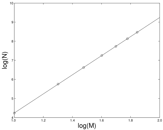
Figure 1: Total number of vacua, $N$, as a function of the range of flux/torsion parameters, $M$ (in logarithmic units).

In Figure 1 we have plotted the total number of solutions with $|W_{0}|<1$ (i.e. taking $w=1$ in equation (5.14)) for $M=10,20,\dots,70$.

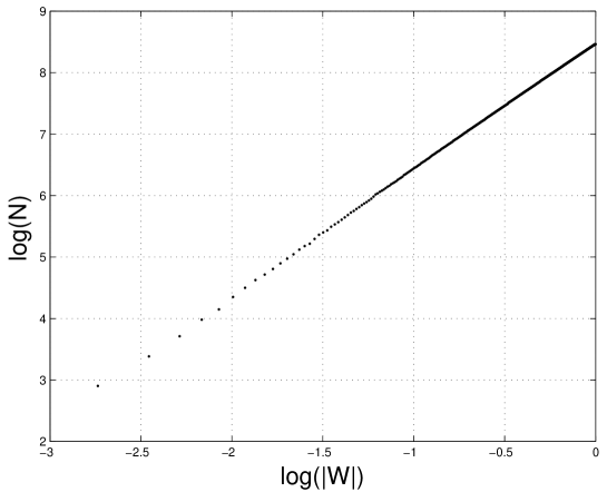
Figure 2: Number of vacua $N$ with $|{\cal W}_{0}|<w$ as a function of $w$ (in logarithmic units), for flux/torsion parameters in the range $-70,\dots,70$.

In Figure 2 we have presented the result for $N(70,w)$, the number of vacua in the flux/torsion range from $-70,\dots,70$, as a function of the superpotential value, $|W|$. The numerical value of $x$ can be easily understood intuitively. Although we consider a model with seven parameters, the requirement of small $\mathrm{Re}({\cal W}_{0})$ and small $\mathrm{Im}({\cal W}_{0})$ effectively fixes two of these parameters, leading to a scaling law with power $5$. We also remark that the value of $y$ close to $y=2$ corresponds to a nearly uniform random distribution of ${\cal W}_{0}$ values in the complex ${\cal W}_{0}$ plane.

As can be seen from Figure 2, $|{\cal W}_{0}|$ values of $0.01$ and smaller can be obtained. Our result gives an indication of what fraction of vacua leads to a gauge coupling of $s\simeq 24$ as suggested by gauge unification in the MSSM. Assuming the $E_{8}$ beta-function coefficient (3.14) such a value for $s$ translates into $x\simeq 5$ which, from Eq. (5.6) (setting $k=1$ for simplicity) implies $|{\cal W}_{0}|\simeq 1/14$ (or, equivalently, ${\rm log}|{\cal W}_{0}|\simeq-1.15$). This means approximately a fraction of $10^{-3}$ of all vacua with $|{\cal W}_{0}|<1$ lead a gauge coupling sufficiently weak to be compatible with gauge unification. For a condensing gauge group smaller than $E_{8}$ or a value of $k$ smaller than one this fraction will decrease accordingly.

We have also checked the case $r\neq 0$ without the constraint (5.10) and the results are similar to the one obtained for $r=0$.

Finally we would like to show a numerical proof of the validity of our procedure (i.e. the use of the global SUSY condition ${\cal W}_{i}(T_{0},Z_{0})={\cal W}_{a}(T_{0},Z_{0})=0$ with $|{\cal W}_{0}/M_{0}|\ll 1$ in order to find an approximate solution for the $T$ and $Z$ fields). We have chosen, within this $r=0$ case, values for the flux/torsion parameters as follows

$$e=-7\;,\ \epsilon=-4\;,\ \mu=2\;,\ \rho=5\;,\ p=1\;,\ q=2\;,\ \xi=-13\;,$$ (5.16)

for which Eqs (5.13) give the field values

$$z_{0} = 2.598\;,$$

$$t_{0} = 2.165\;,$$

$$\zeta_{0} = 0.500\;,$$ (5.17)

$$\tau_{0} = 2.250\;,$$

with $|{\cal W}_{0}|=0.167$. As it is illustrated in Figure 3, these values are very close to the actual solution to the F-equations, given by

$$z_{0} = 2.598\;,$$

$$t_{0} = 2.164\;,$$

$$\zeta_{0} = 0.520\;,$$ (5.18)

$$\tau_{0} = 2.300\;.$$

Using the beta-function coefficient (3.14) and $k=2$, the values for the dilaton field are found to be

$$s= 23.190\;,$$ (5.19)

$$\sigma= 22.399\;,$$

which proves that phenomenologically viable values for the gauge coupling can be obtained for reasonable values of the flux parameters.

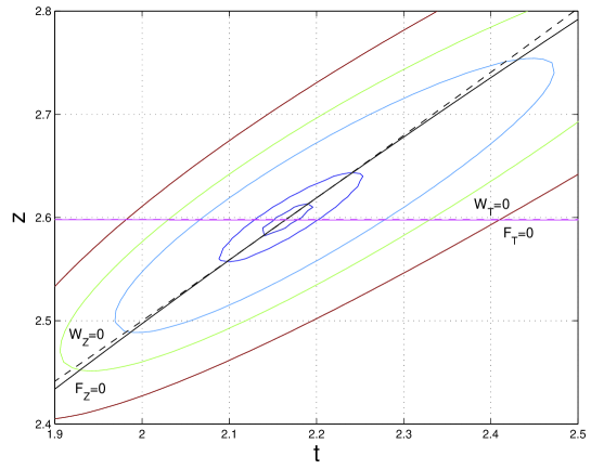
Figure 3: Contour plot of the potential, on the $(t,z)$ plane, for the example shown in the text, Eq. (5.16). The solid (dashed) lines are the $\mathrm{Re}(F_{T})=\mathrm{Re}(F_{Z})=0$ ($\mathrm{Re}(W_{T})=\mathrm{Re}(W_{Z})=0$) local (global) SUSY conditions. Note that the lines ${\rm Re}(W_{T})=0$ and ${\rm Re}(F_{T})=0$ coincide.

We should add that we have computed the Hessian matrix for this example and we have explicitly checked that all eigenvalues are positive at the point where the F-equations vanish. This is quite important as the potential at the minimum is negative, actually given by $V=-3{\rm e}^{K}|{\cal W}_{0}|^{2}$, and very small, of the order of 10^-7. This means that, in a small region around the true minimum, the potential will shift from negative to positive values and, this being a multi-variable potential, it is easy to get mistaken about the real position of the minimum. For example, if we were to use the global supersymmetric solution given by (5.17), due to its closeness to the real one, (5.18), the no-scale cancellation mechanism would take place and the scalar potential would read, at this point, $V=+3{\rm e}^{K}|{\cal W}_{0}|^{2}$. That is, we would predict a dS vacuum (of order 10^-7) were, in reality, the only minimum in that region is AdS.

Before we conclude this section we would like to make a few comments about the general case, with an arbitrary numbers of moduli fields. As it is evident from (2.30) and (2.27), the number of parameters grows rapidly with the number of fields, making a numerical search for vacua infeasible. We have, therefore, not attempted to extend the numerical analysis beyond the three-field STZ model. However, the experience with this model shows that dropping the constraint (3.9) is crucial in order to obtain small values of $|{\cal W}_{0}|$ and we expect this to be true in general. Conversely, multi-field models without the constraint (3.9) should be at least as flexible as their three-field counterpart and should, therefore, allow small $|{\cal W}_{0}|$ values without problems. From our general argument relating globally and locally supersymmetric vacua, this should then allow consistent, locally supersymmetric vacua at weak coupling as determined by Eq. (5.6). As for the scaling law (5.14), in the general case one would expect scaling powers $x\simeq n-2$, where $n$ is the total number of parameters in the model and $y\simeq 2$, leading to the same uniform random distribution in the ${\cal W}$ plane which we have observed in the STZ model.

6 Conclusion

In this paper we have analyzed the vacuum properties of various classes of heterotic models on certain manifolds with SU(3) structure. After a review of the heterotic string on half-flat mirror manifolds [32], defined by (2.20), we have derived the superpotential for a more general class of manifolds with SU(3) structure which were introduced in Refs [34, 35, 36]. We have explicitly verified in these models that the application of the heterotic Gukov-Vafa-Witten type formula for the superpotential leads to the same result as an explicit reduction of the ten-dimensional bosonic terms. The resulting superpotential, which is given in Eqs (2.30), (2.27), resembles very much the one obtained in type IIB orientifold compactifications suggesting that one may recover the flexibility of type II models in the heterotic case. These flux/torsion superpotentials depend on $h^{(1,1)}$ Kähler moduli $T^{i}$ as well as on $h^{(2,1)}$ complex structure moduli $Z^{a}$, but are independent of the dilaton $S$. We have, therefore, supplemented our superpotential with a contribution from hidden sector gaugino condensation in order to stabilize the dilaton, which is again similar to the type IIB constructions where non-perturbative terms need to be added in order to fix the Kähler moduli.

We have first analyzed moduli stabilization for the models based on half-flat mirror manifolds and have found a number of problems. Generally in those models, $h^{(1,1)}+h^{(2,1)}-1$ axion directions remain flat, and it is hard to achieve the large radius and large complex structure limits as well as weak gauge coupling. In models with additional magnetic torsion terms, the flat axion directions are lifted and moderately weak coupling can be achieved, while stabilizing field in the large radius and large complex structure limits remains a problem. However, such models with additional magnetic torsion terms, although a plausible extension of half-flat mirror models, cannot currently be derived within the heterotic string.

We have traced the root cause of the aforementioned problems to the fact that the flux/torsion superpotential ${\cal W}$ is too simple to allow for globally supersymmetric vacua. Consequently, we have analyzed moduli stabilization for some generalised half-flat models whose associated superpotential is significantly more complicated. We have seen that consistent weak-coupling vacua can be obtained if the flux/torsion superpotential has globally supersymmetric vacua with a superpotential value ${\cal W}_{0}$ satisfying $|{\cal W}_{0}|\ll 1$. The value of the dilaton and, hence, the gauge coupling, is then directly related to $|{\cal W}_{0}|$. We have verified that the superpotential for the generalised half-flat models has indeed globally supersymmetric vacua with all Kähler and complex structure moduli stable. However, the requirement of small $|{\cal W}_{0}|$ turned out to be more subtle. For the standard embedding of the spin connection into the gauge group, the resulting Bianchi identity $d{\hat{H}}=0$ for the NSNS form led to a constraint (3.9) on the flux/torsion parameters which ruled out the possibility of small ${\cal W}_{0}$, at least within the range of flux/torsion parameters covered by our numerical scan. However, for more general gauge bundles, the constraint should be dropped and vacua with small $|{\cal W}_{0}|$ can easily be obtained in this case. The number of such vacua as a function of $|{\cal W}_{0}|$ for a simple model with three fields, $S$, $T$ and $Z$, has been plotted in Figure 2. Using Eq. (5.6) one can estimate that, typically, the fraction of vacua that lead to a sufficiently weak gauge coupling consistent with gauge unification, is $10^{-3}$. Our results establish the existence of consistent, weak-coupling AdS vacua within generalised heterotic half-flat models.

In the light of these results, it is clearly desirable to get to a better understanding of half-flat compactifications and their generalizations, in particular with regard to the precise nature of the manifolds involved, the rules for quantizing flux and torsion parameters in those compactifications and the inclusion of gauge and gauge matter fields. We will leave those tasks for future publications.

Acknowledgments We would like to thank Nuno Antunes, Kiwoon Choi, Jan Louis, Hans–Peter Nilles and Silvia Vaulà for helpful discussions. BdC, AL and AM are supported by PPARC. SG is supported by the JSPS under contract P03743.

Appendix

Appendix A Ricci scalar for the “extended half-flat” manifolds

This section contains a generalization of the result obtained in the appendices of Ref. [33], where the Ricci scalar for half-flat manifolds mirror to Calabi-Yau with NS-NS fluxes was computed. Here we will follow this calculation closely, by recalling the main identities which remain valid, while pointing out the places where it differs from the simple half-flat case.

To set the stage, let us briefly recall a few features of manifolds with SU(3) structure. Such manifolds are characterized by the existence of an almost complex structure with the associated fundamental form $J$ and a $(3,0)$ complex form $\Omega$ which are invariant under the action of the SU(3) structure group. More concretely this means that the forms $J$ and $\Omega$ are covariantly constant with respect to some connection $\nabla^{(T)}$, which in general has a torsion. Decomposed into SU(3) representations the torsion falls into five different classes $\mathcal{W}_{1}\;,\ \ldots,\mathcal{W}_{5}$ which are given by

$$dJ = \mathcal{W}_{1}\Omega+\mathcal{W}_{4}\wedge J+\mathcal{W}_{3}\;,$$ (A.1)

$$d\Omega = \mathcal{W}_{1}J\wedge J+\mathcal{W}_{5}\wedge\Omega+\mathcal{W}_{2}\;.$$

Since the torsion on manifolds with SU(3) structure measures the departure from Calabi–Yau manifolds (which are Ricci flat) it is clear that the Ricci scalar of the SU(3) structure manifolds depends on their torsion. Thus, in order to compute the Ricci scalar, we will need to know all the components of the torsion and for this we will use equations (A.1) above and the relations

$$d\Omega = E_{i}\tilde{\omega}^{i}\;,$$ (A.2)

$$dJ = (t^{i}p_{Ai})\beta^{A}-(t^{i}q_{i}^{A})\alpha_{A}\;,$$ (A.3)

which are easily derived from (2.4) and (2.21), with the quantities $E_{i}$ defined in equation (2.34). Note we have postulated that the basis forms in the above equations have the same SU(3) properties as their Calabi–Yau counterparts. Hence, $\alpha_{A}$ and $\beta^{A}$ in Eq. (2.21) are primitive and, consequently, $\mathcal{W}_{4}$ has to vanish. Moreover as $d\Omega$ in Eq. (A.2) is a $(2,2)$ form, $\mathcal{W}_{5}$ also vanishes. The other torsion components $T_{1+2}$ and $T_{3}$ are found to be

$$(T_{1+2})_{\alpha\beta\gamma} = \frac{\bar{E}_{i}}{4||\Omega||^{2}}(\tilde{\omega}^{i})_{\alpha\beta\bar{\alpha}\bar{\beta}}\Omega^{\bar{\alpha}\bar{\beta}}{}_{\gamma}\;,$$ (A.4)

$$(T_{3})_{\alpha\beta\bar{\gamma}} = -\frac{i}{2}t^{i}(p_{Ai}\beta^{A}_{\alpha\beta\bar{\gamma}}-q_{i}^{A}\alpha_{A\alpha\beta\bar{\gamma}})\;.$$ (A.5)

Here $||\Omega||^{2}=\frac{1}{6}\Omega_{\alpha\beta\gamma}{\bar{\Omega}}^{\alpha\beta\gamma}$ is a function of the complex structure moduli which is related to the Kähler potential for these fields via ${\cal V}||\Omega||^{2}=e^{-K^{(Z)}}$, where ${\cal V}$ is the volume of the manifold. Note that, in this case, the quantities $E_{i}$ are neither real nor constants as it happened for the case of half-flat manifolds and thus one generically has

$$T\in\mathcal{W}_{1}\oplus\mathcal{W}_{2}\oplus\mathcal{W}_{3}\;.$$ (A.6)

However it is important to note that the nature of the indices of the torsion components is the same as in the half-flat case, and the torsion itself is still traceless. As a consequence, the expression of the Ricci scalar in terms of the torsion obtained in [33] still holds

$$R=(T_{1+2})_{\alpha\beta\gamma}(T_{1+2})^{\alpha\beta\gamma}-6(T_{1+2})_{\alpha\beta\gamma}(T_{1+2})^{\beta\gamma\alpha}+(T_{3})_{\alpha\beta\bar{\gamma}}(T_{3})^{\alpha\beta\bar{\gamma}}+{\rm c.c.}$$ (A.7)

To obtain the integrated Ricci scalar we perform the same steps as in Ref. [33] and, using the relations (B), we obtain

$$\int_{\hat{X}}\sqrt{g}\,R = {\rm e}^{K^{(}Z)}(g^{ij}E_{i}\bar{E}_{j}-4t^{i}t^{j}E_{i}\bar{E}_{j})$$ (A.8)

$$-\frac{1}{2}t^{i}t^{j}(p_{Ai}-q_{i}^{C}\mathcal{M}_{CA})\big{(}\mathrm{Im}\mathcal{M}^{-1}\big{)}^{AB}(p_{Bj}-q_{j}^{D}\bar{\mathcal{M}}_{BD})\;.$$

After taking into account various coefficients and rescalings, the contribution of gravity to the potential in Einstein’s frame can be rewritten as

$$e^{-K}V_{g} = 8(g^{ij}E_{i}\bar{E}_{j}-4t^{i}t^{j}E_{i}\bar{E}_{j})$$

$$-4e^{-K^{(Z)}}\big{[}\mathrm{Im}(\tilde{\epsilon}_{A})-\mathrm{Im}(\tilde{\mu}^{C})\mathcal{M}_{CA}\big{]}\big{(}\mathrm{Im}\mathcal{M}^{-1}\big{)}^{AB}\big{[}\mathrm{Im}(\tilde{\epsilon}_{B})-\mathrm{Im}(\tilde{\mu}^{D})\bar{\mathcal{M}}_{DB}\big{]}\;.$$

Appendix B Some useful results on special geometry

As it is well known, the moduli space of Calabi–Yau manifolds splits into a product of two special Kähler manifolds, one for the complexified Kähler class deformations and one for the complex structure deformations. Since these geometries are at the heart of the four-dimensional physics obtained from compactifications on Calabi–Yau manifolds we review in this appendix some of the properties of the special Kähler manifolds which we need in the main part of the paper. We mainly follow Ref. [43].

The main feature of special Kähler manifolds is that their geometry is completely determined in terms of a holomorphic function $\mathcal{H}$, called the pre-potential. In terms of the projective coordinates $\mathcal{X}^{P}$, where $P=0,\ldots,n$ ($n$ being the complex dimension of the manifold), the pre-potential is a homogeneous function of degree two, that is, it satisfies $\mathcal{X}^{P}\mathcal{H}_{P}=2\mathcal{H}$, where $\mathcal{H}_{P}=\frac{\partial}{\partial\mathcal{X}^{P}}\mathcal{H}$. In fact, one does not always need to rely on the pre-potential and it may be sufficient to work with the period vector

$$\mathcal{O}=\left(\begin{array}[h]{c}\mathcal{X}^{P}\\ \mathcal{H}_{P}\\ \end{array}\right).$$ (B.1)

Let us further introduce the symplectic inner product $<,>$ as

$$<\mathcal{O},\bar{\mathcal{O}}>\equiv\mathcal{O}^{T}\left(\begin{array}[]{cc}0&-\mathbf{1}\\ \mathbf{1}&0\end{array}\right)\bar{\mathcal{O}}=(\mathcal{H}_{P}\bar{\mathcal{X}}^{P}-\bar{\mathcal{H}}_{P}\mathcal{X}^{P})\;.$$ (B.2)

With this notation the Kähler potential can be written as

$$K=-\log{\big{(}i<\mathcal{O},\bar{\mathcal{O}}>\big{)}}=-\log{\big{[}i(\mathcal{H}_{P}\bar{\mathcal{X}}^{P}-\bar{\mathcal{H}}_{P}\mathcal{X}^{P})\big{]}}\;,$$ (B.3)

while the Kähler metric is given by the usual formula

$$g_{p\bar{q}}=\partial_{p}{\bar{\partial}}_{\bar{q}}K\;.$$ (B.4)

Here the derivatives are with respect to the affine coordinates $X^{p}=\mathcal{X}^{p}/\mathcal{X}^{0}$, where $p,q,\dots=1,\dots,n$. It is also useful to introduce the Kähler covariant derivative of the periods $\mathcal{O}$

$$e^{-K/2}U_{q}\equiv e^{-K/2}\left(\begin{array}[]{c}f_{q}^{P}\\ h_{P\;q}\\ \end{array}\right)=\nabla_{p}\mathcal{O}=(\partial_{p}+\partial_{p}K)\mathcal{O}\;.$$ (B.5)

The period matrix $\mathcal{Q}$, which is a complex symmetric matrix is now required to satisfy

$$\bar{\mathcal{H}}_{P}= {\bar{\mathcal{Q}}}_{PQ}{\bar{\mathcal{X}}}^{Q}\;,$$ (B.6)

$$h_{P\;q}= {\bar{\mathcal{Q}}}_{PS}f_{q}^{S}\;.$$

It can be shown, see Ref [44], that, in terms of the pre-potential $\mathcal{H}$, the period matrix has the form

$$\mathcal{Q}_{PQ}=\bar{\mathcal{H}}_{PQ}+2i\frac{(\mathrm{Im}\mathcal{H})_{PR}(\mathrm{Im}\mathcal{H})_{QS}\mathcal{X}^{R}\mathcal{X}^{S}}{(\mathrm{Im}\mathcal{H})_{RS}\mathcal{X}^{R}\mathcal{X}^{S}}\;,$$ (B.7)

where we have denoted $\mathcal{H}_{RS}=\frac{\partial}{\partial\mathcal{X}^{R}}\frac{\partial}{\partial\mathcal{X}^{S}}\mathcal{H}$.

With this one can prove the following relations

$$<\mathcal{O},U_{p}> = <\mathcal{O},\bar{U}_{\bar{p}}>=0\;,$$

$$g_{p\bar{q}} = -i<U_{p},\bar{U}_{\bar{q}}>=-2f_{p}^{P}\mathrm{Im}\mathcal{Q}_{PQ}{\bar{f}}_{\bar{q}}^{Q}\;,$$ (B.8)

$$f_{p}^{P}{\bar{f}}_{\bar{q}}^{Q}g^{p\bar{q}} = -\frac{1}{2}(\mathrm{Im}\mathcal{Q})^{-1\;PQ}-e^{K}{\bar{\mathcal{X}}}^{P}\mathcal{X}^{Q}\;.$$

In order to make this discussion less abstract let us first apply the above formalism to the complex structure moduli space of Calabi–Yau manifolds. The periods $\mathcal{O}$ are now determined by the holomorphic $(3,0)$ form $\Omega$. Moreover the inner product (B.2) becomes now the inner product for three-forms on the Calabi–Yau manifold. With this one immediately finds that the Kähler potential (B.3) precisely reproduces the one from equation (2.14). Finally, the Kähler covariant derivatives in equation (B.5) give the components of the $(2,1)$ forms in the basis (2.2). With these identifications it is easy to see that most of the relations in equation (B) are straightforward, the only non-trivial ones involving the period matrix. Denoting the period matrix by $\mathcal{M}$ in this case and the indices $P,Q,\ldots$ by $A,B,\ldots=1,\ldots,h^{(2,1)}$, the last relations in equation (B) become

$$g_{a\bar{b}} = -2f_{a}^{A}\mathrm{Im}\mathcal{M}_{AB}{\bar{f}}_{\bar{b}}^{B}\;,$$

$$e^{K}D_{a}Z^{A}D_{\bar{b}}{\bar{Z}}^{B}=f_{a}^{A}{\bar{f}}_{\bar{b}}^{B}g^{a\bar{b}} = -\frac{1}{2}(\mathrm{Im}\mathcal{M})^{-1\;AB}-e^{K}{\bar{Z}}^{A}Z^{B}\;.$$ (B.9)

Finally we note that in the basis (2.2) the period matrix $\mathcal{M}$ can be found to be

$$\int_{Y_{3}}\alpha_{A}\wedge*\beta^{B} = -(\mathrm{Re}\mathcal{M})_{AC}(\mathrm{Im}\mathcal{M})^{-1\;CB}\;,$$

$$\int_{Y_{3}}\alpha_{A}\wedge*\alpha_{A} = -(\mathrm{Im}\mathcal{M})_{AB}-(\mathrm{Re}\mathcal{M})_{AC}(\mathrm{Im}\mathcal{M})^{-1\;CD}(\mathrm{Re}\mathcal{M})_{DB}\;,$$ (B.10)

$$\int_{Y_{3}}\beta^{A}\wedge*\beta^{B} = -(\mathrm{Im}\mathcal{M})^{-1\;AB}\;.$$

While the pre-potential is typically a complicated function it simplifies considerably in certain limits in moduli space, such as large radius and large complex structure limits for the Kähler and complex structure moduli spaces, respectively. In those limits, the pre-potential is given by a cubic function

$$\mathcal{H}=-\frac{1}{6}\frac{d_{pqr}\mathcal{X}^{p}\mathcal{X}^{p}\mathcal{X}^{r}}{\mathcal{X}^{0}}\;,$$ (B.11)

Such a cubic pre-potential defines what is known as very special geometry. Writing the affine coordinates as

$$X^{p}=\xi^{p}+ix^{p}\;,$$ (B.12)

one finds for the Kähler potential

$$K=-\ln\left(\frac{4}{3}\mathcal{K}\right)\;,$$ (B.13)

where

$$\mathcal{K}=\frac{i}{8}d_{pqr}(X^{p}-\bar{X}^{p})(X^{q}-\bar{X}^{q})(X^{r}-\bar{X}^{r})=d_{pqr}x^{i}x^{j}x^{k}\;.$$ (B.14)

From equation (B.7) one can also define a period matrix in this case and then the relations (B) follow by straightforward algebraic manipulations. There are a number of further very special geometry relations which are useful in the main part of this paper. First, let us define

$$\mathcal{K}_{p}=d_{pqr}x^{q}x^{r}\;,\qquad\mathcal{K}_{pq}=d_{pqr}x^{r}\;.$$ (B.15)

With this, the first derivatives of the Kähler potential $K$ with respect to $X^{p}$, denoted by $K_{p}$ and the Kähler metric $K_{p\bar{q}}$ can be written as

$$K_{p} = -\frac{3i\mathcal{K}_{p}}{2\mathcal{K}}\;,$$ (B.16)

$$g_{pq} = K_{p\bar{q}}=-\frac{3}{2}\left(\frac{\mathcal{K}_{pq}}{\mathcal{K}}-\frac{3\mathcal{K}_{p}\mathcal{K}_{q}}{2\mathcal{K}^{2}}\right)\;.$$ (B.17)

Defining fields $x_{p}=g_{pq}x^{q}$ with lowered indices it is easy to show that

$$x_{p}=\frac{3\mathcal{K}_{p}}{4\mathcal{K}}\;,\qquad x_{p}x^{p}=\frac{3}{4}\;.$$ (B.18)

These formulae lead immediately to the “no-scale” relation

$$K^{p\bar{q}}K_{p}{\bar{K}}_{\bar{q}}=3\;.$$ (B.19)

Finally we note that a typical flux superpotential, for example as it arises from the Gukov-Vafa-Witten formula, can be written as

$$W=e_{P}\mathcal{X}^{P}-m^{P}\mathcal{H}_{P}\;.$$ (B.20)

Here $e_{P}$ and $m^{P}$ depend on the fluxes and can be either real constants or can also depend holomorphically on other (super)fields in the theory, but not on $X^{p}$, as we have seen in section 2.2. For the cubic pre-potential (B.11) the dependence on the physical degrees of freedom $X^{p}$ can be made explicit after setting $\mathcal{X}^{0}$ to one and we find

$$W=e_{0}+e_{p}X^{p}+\frac{1}{2}d_{pqr}m^{p}X^{q}X^{r}-\frac{m^{0}}{6}d_{pqr}X^{p}X^{q}X^{r}\;.$$ (B.21)

Note that after transforming to the “phenomenological” convention for $X^{p}$ by $X^{p}\rightarrow-iX^{p}$ (and after dropping an overall factor of $-i$ from $W$ which is irrelevant) the constant and quadratic terms in the above superpotential pick up a factor of $i$.

Appendix C Supergravity conventions in $d=4$ and stability of supersymmetric vacua

In this appendix we summarize conventions and relevant formulae for four-dimensional $N=1$ supergravity [45]. Further, we present an elementary proof that solutions to the F-equations are always stable vacua.

The bosonic terms in the action of four-dimensional $N=1$ supergravity coupled to chiral fields $(\phi^{X})=(S,T^{i},Z^{a})$ read

$$S=-\frac{1}{\kappa_{4}^{2}}\int_{M_{4}}\sqrt{-g}\;d^{4}x\;\left[\frac{1}{2}R+K_{XY}\partial_{\mu}\phi^{X}\partial^{\mu}\bar{\phi}^{Y}+V\right]\;,$$ (C.1)

where $\kappa_{4}$ is the four-dimensional Newton constant. As usual, $K_{XY}=\partial_{X}\partial_{Y}K$ is the Kähler metric while the potential $V$ is given by the standard formula

$$V=e^{K}\left(K^{XY}F_{X}\bar{F}_{Y}-3|W|^{2}\right)\;,$$ (C.2)

where $K^{XY}$ is the inverse Kähler metric and the F-terms $F_{X}$ are defined by

$$F_{X}=W_{X}+K_{X}W\;.$$ (C.3)

Here a subscript $X$ denotes a derivative with respect to $\phi^{X}$, as usual. Note that we have considered the chiral fields and the Kähler potential to be dimensionless, while the superpotential has dimension one, a convention which is convenient for the discussion of moduli fields and in line with the formulae in the main part of the paper.

In this paper we were interested in supersymmetric vacua of the potential (C.2), that is, vacua which can be obtained by solving the F-equations

$$F_{X}=W_{X}+K_{X}W=0\;.$$ (C.4)

It is easy to show, from Eq. (C.2), that solutions to the F-equations indeed constitute extremal points of the potential $V$. The cosmological constant, $V_{0}$, at such an extremal point is given by

$$V_{0}=-3e^{K}|W|^{2}\;.$$ (C.5)

Without fine-tuning (to make $W$ at the extremal point vanish) this value will usually be negative and, hence, we are generically dealing with AdS vacua. The stability of AdS vacua in gravity coupled to scalar fields was analyzed a long time ago [46, 47] by Breitenlohner and Freedman and, independently, by Abbott and Deser. They found that such vacua are stable if all scalar field masses are larger than a certain lower bound, which is basically given by the cosmological constant $V_{0}$. Hence in AdS space, unlike in Minkowski space, negative (square) masses do not necessarily indicate an instability. In fact, it can be shown in general, [41], that this bound is always satisfied for supersymmetric vacua of supergravity theories and, hence, such vacua are always stable. We will now present an elementary proof of this statement.

Let us first formulate the Breitenlohner-Freedman bound for a theory with canonically normalized real scalars $\chi^{i}$ and a potential $V=V(\chi^{i})$. We assume the potential has a stationary point at $\chi^{i}=\chi^{i}_{0}$ with negative cosmological constant $V_{0}=V(\chi^{i}_{0})<0$. Define the mass matrix as

$$M_{ij}=\frac{\partial^{2}V}{\partial\chi^{i}\partial\chi^{j}}(\chi^{k}_{0})\;.$$ (C.6)

According to Breitenlohner and Freedman this stationary point leads to a stable, AdS vacuum if $a_{i}\geq 3V_{0}/2$, where $a_{i}$ are the eigenvalues of $M$. A sufficient criterion for this to be the case is that

$$\xi^{T}M\xi-\frac{3}{2}V_{0}\xi^{T}\xi\geq 0\;,$$ (C.7)

for all vectors $\xi$ in field space. To see that this inequality implies the one for the eigenvalues, choose $\xi$ to be the eigenvectors of the mass matrix $M$. It is useful for the application to supergravity to re-write this criterion for non-canonical kinetic terms $G_{ij}\partial_{\mu}\chi^{i}\partial^{\mu}\chi^{j}$, where $G_{ij}$ is the metric on field space. Then, Eq. (C.7) takes the form

$$\xi^{T}M\xi-\frac{3}{2}V_{0}\xi^{T}G\xi\geq 0\;,$$ (C.8)

where the mass matrix $M$ is now, of course, defined with respect to the non-canonical fields.

We would like to apply the criterion (C.8) to the case of four-dimensional $N=1$ supergravity with complex scalars $\phi^{X}$, Kähler potential $K$ and superpotential $W$. We consider a solution $\phi_{0}^{X}$ of the F-equations (C.4). This solution is automatically a stationary point of the potential $V$ and it preserves supersymmetry. The cosmological constant $V_{0}$ at such a vacuum is given by Eq. (C.5). From Eq. (C.2) one finds for the second derivatives of $V$ at $F_{X}=0$ after a bit of computation

$$\left.V_{XY}\right|_{F=0} = -e^{K}\bar{W}F_{XY}\;,$$ (C.9)

$$\left.V_{X\bar{Y}}\right|_{F=0} = e^{K}\left[K^{Z\bar{T}}F_{ZX}\bar{F}_{\bar{T}\bar{Y}}-2K_{X\bar{Y}}|W|^{2}\right]\;,$$ (C.10)

where $F_{XY}$ is the derivative of $F_{X}$ with respect to $\phi^{Y}$. Combining these results (and taking care to convert real into complex expressions) it is then straightforward to compute the LHS of the criterion (C.8) which takes the form

$$2V_{X\bar{Y}}\xi^{X}\xi^{\bar{Y}}+V_{XY}\xi^{X}\xi^{Y}+V_{\bar{X}\bar{Y}}\xi^{\bar{X}}\xi^{\bar{Y}}-\frac{3}{2}V_{0}K_{X\bar{Y}}\xi^{X}\xi^{\bar{Y}}$$ (C.11)

$$= e^{K}\left[2K^{Z\bar{T}}F_{ZX}\bar{F}_{\bar{T}\bar{Y}}\xi^{X}\xi^{\bar{Y}}-\bar{W}F_{XY}\xi^{X}\xi^{Y}-W\bar{F}_{\bar{X}\bar{Y}}\xi^{\bar{X}}\xi^{\bar{Y}}+\frac{1}{2}|W|^{2}K_{X\bar{Y}}\xi^{X}\xi^{\bar{Y}}\right]$$

$$= e^{K}\left(\frac{1}{\sqrt{2}}WK_{Z\bar{X}}\xi^{\bar{X}}-\sqrt{2}F_{ZX}\xi^{X}\right)K^{Z\bar{T}}\left(\frac{1}{\sqrt{2}}\bar{W}K_{\bar{T}Y}\xi^{Y}-\sqrt{2}\bar{F}_{\bar{T}\bar{Y}}\xi^{\bar{Y}}\right)\;.$$

The last line is obviously positive and, hence, the criterion is satisfied. The conclusion is that any supersymmetric AdS vacuum of four-dimensional $N=1$ supersymmetry satisfies the Breitenlohner/Freedman criterion and, therefore, constitutes a stable AdS vacuum.

References

- [1] S. B. Giddings, S. Kachru and J. Polchinski, “Hierarchies from fluxes in string compactifications,” Phys. Rev. D 66 (2002) 106006 [arXiv:hep-th/0105097].
- [2] S. Kachru, R. Kallosh, A. Linde and S. P. Trivedi, “De Sitter vacua in string theory,” Phys. Rev. D 68 (2003) 046005 [arXiv:hep-th/0301240].
- [3] K. Becker, M. Becker, M. Haack and J. Louis, “Supersymmetry breaking and alpha’-corrections to flux induced potentials,” JHEP 0206 (2002) 060 [arXiv:hep-th/0204254].
- [4] V. Balasubramanian and P. Berglund, “Stringy corrections to Kaehler potentials, SUSY breaking, and the cosmological constant problem,” JHEP 0411 (2004) 085 [arXiv:hep-th/0408054].
- [5] K. Choi, A. Falkowski, H. P. Nilles, M. Olechowski and S. Pokorski, “Stability of flux compactifications and the pattern of supersymmetry breaking,” JHEP 0411 (2004) 076 [arXiv:hep-th/0411066].
- [6] V. Balasubramanian, P. Berglund, J. P. Conlon and F. Quevedo, “Systematics of moduli stabilisation in Calabi-Yau flux compactifications,” JHEP 0503 (2005) 007 [arXiv:hep-th/0502058].
- [7] J. P. Conlon, F. Quevedo and K. Suruliz, “Large-volume flux compactifications: Moduli spectrum and D3/D7 soft supersymmetry breaking,” arXiv:hep-th/0505076.
- [8] D. Lust, S. Reffert, W. Schulgin and S. Stieberger, “Moduli stabilization in type IIB orientifolds. I: Orbifold limits,” arXiv:hep-th/0506090.
- [9] S. P. de Alwis, “On integrating out heavy fields in SUSY theories,” arXiv:hep-th/0506267.
- [10] S. P. de Alwis, “Effective potentials for light moduli,” arXiv:hep-th/0506266.
- [11] T. R. Taylor and C. Vafa, “RR flux on Calabi-Yau and partial supersymmetry breaking,” Phys. Lett. B 474 (2000) 130 [arXiv:hep-th/9912152].
- [12] J. Louis and A. Micu, “Type II theories compactified on Calabi-Yau threefolds in the presence of background fluxes,” Nucl. Phys. B 635 (2002) 395 [arXiv:hep-th/0202168].
- [13] T. W. Grimm and J. Louis, “The effective action of type IIA Calabi-Yau orientifolds,” Nucl. Phys. B 718 (2005) 153 [arXiv:hep-th/0412277].
- [14] J. P. Derendinger, C. Kounnas, P. M. Petropoulos and F. Zwirner, “Superpotentials in IIA compactifications with general fluxes,” Nucl. Phys. B 715 (2005) 211 [arXiv:hep-th/0411276].
- [15] O. DeWolfe, A. Giryavets, S. Kachru and W. Taylor, “Type IIA moduli stabilization,” arXiv:hep-th/0505160.
- [16] G. Villadoro and F. Zwirner, “N = 1 effective potential from dual type-IIA D6/O6 orientifolds with general fluxes,” JHEP 0506 (2005) 047 [arXiv:hep-th/0503169].
- [17] T. House and E. Palti, “Effective action of (massive) IIA on manifolds with SU(3) structure,” arXiv:hep-th/0505177.
- [18] P. G. Camara, A. Font and L. E. Ibanez, “Fluxes, moduli fixing and MSSM-like vacua in a simple IIA orientifold,” arXiv:hep-th/0506066.
- [19] P. Candelas, G. T. Horowitz, A. Strominger and E. Witten, “Vacuum Configurations For Superstrings,” Nucl. Phys. B 258 (1985) 46.
- [20] M. Dine, R. Rohm, N. Seiberg and E. Witten, “Gluino Condensation In Superstring Models,” Phys. Lett. B 156 (1985) 55.
- [21] R. Rohm and E. Witten, “The Antisymmetric Tensor Field In Superstring Theory,” Annals Phys. 170 (1986) 454.
- [22] S. Gukov, S. Kachru, X. Liu and L. McAllister, “Heterotic moduli stabilization with fractional Chern-Simons invariants,” Phys. Rev. D 69 (2004) 086008 [arXiv:hep-th/0310159].
- [23] G. Curio, A. Krause and D. Lust, “Moduli stabilization in the heterotic / IIB discretuum,” arXiv:hep-th/0502168.
- [24] G. L. Cardoso, G. Curio, G. Dall’Agata, D. Lust, P. Manousselis and G. Zoupanos, “Non-Kaehler string backgrounds and their five torsion classes,” Nucl. Phys. B 652 (2003) 5 [arXiv:hep-th/0211118].
- [25] K. Becker, M. Becker, K. Dasgupta and P. S. Green, “Compactifications of heterotic theory on non-Kaehler complex manifolds. I,” JHEP 0304 (2003) 007 [arXiv:hep-th/0301161].
- [26] K. Becker, M. Becker, K. Dasgupta and S. Prokushkin, “Properties of heterotic vacua from superpotentials,” Nucl. Phys. B 666 (2003) 144 [arXiv:hep-th/0304001].
- [27] G. L. Cardoso, G. Curio, G. Dall’Agata and D. Lust, “BPS action and superpotential for heterotic string compactifications with fluxes,” JHEP 0310 (2003) 004 [arXiv:hep-th/0306088], G. L. Cardoso, G. Curio, G. Dall’Agata and D. Lust, “Heterotic string theory on non-Kaehler manifolds with H-flux and gaugino condensate,” Fortsch. Phys. 52 (2004) 483 [arXiv:hep-th/0310021].
- [28] K. Becker, M. Becker, P. S. Green, K. Dasgupta and E. Sharpe, “Compactifications of heterotic strings on non-Kaehler complex manifolds. II,” Nucl. Phys. B 678 (2004) 19 [arXiv:hep-th/0310058].
- [29] M. Serone and M. Trapletti, “String vacua with flux from freely-acting obifolds,” JHEP 0401 (2004) 012 [arXiv:hep-th/0310245].
- [30] M. Becker and K. Dasgupta, “Kaehler versus non-Kaehler compactifications,” arXiv:hep-th/0312221.
- [31] A. R. Frey and M. Lippert, “AdS strings with torsion: Non-complex heterotic compactifications,” arXiv:hep-th/0507202.
- [32] S. Gurrieri, A. Lukas and A. Micu, “Heterotic string compactified on half-flat manifolds,” Phys. Rev. D 70, 126009 (2004) [arXiv:hep-th/0408121].
- [33] S. Gurrieri, J. Louis, A. Micu and D. Waldram, “Mirror symmetry in generalized Calabi-Yau compactifications,” Nucl. Phys. B 654 (2003) 61 [arXiv:hep-th/0211102].
- [34] R. D’Auria, S. Ferrara, M. Trigiante and S. Vaula, “Gauging the Heisenberg algebra of special quaternionic manifolds,” Phys. Lett. B 610 (2005) 147 [arXiv:hep-th/0410290].
- [35] A. Tomasiello, “Topological mirror symmetry with fluxes,” arXiv:hep-th/0502148.
- [36] M. Grana, J. Louis and D. Waldram, “Hitchin functionals in N = 2 supergravity,” arXiv:hep-th/0505264.
- [37] S. Gukov, C. Vafa and E. Witten, “CFT’s from Calabi-Yau four-folds,” Nucl. Phys. B 584 (2000) 69 [Erratum-ibid. B 608 (2001) 477] [arXiv:hep-th/9906070].
- [38] S. Gukov, “Solitons, superpotentials and calibrations,” Nucl. Phys. B 574 (2000) 169 [arXiv:hep-th/9911011].
- [39] S. Chiossi and S. Salamon, “The Intrinsic Torsion of and Structures,” math.DG/0202282.
- [40] J. Michelson, “Compactifications of type IIB strings to four dimensions with non-trivial classical potential,” Nucl. Phys. B 495 (1997) 127 [arXiv:hep-th/9610151].
- [41] See for example: M. J. Duff, B. E. W. Nilsson and C. N. Pope, “Kaluza-Klein Supergravity,” Phys. Rept. 130 (1986) 1.
- [42] A. Strominger, “Superstrings With Torsion,” Nucl. Phys. B 274 (1986) 253.
- [43] L. Andrianopoli, M. Bertolini, A. Ceresole, R. D’Auria, S. Ferrara, P. Fre and T. Magri, “N = 2 supergravity and N = 2 super Yang-Mills theory on general scalar manifolds: Symplectic covariance, gaugings and the momentum map,” J. Geom. Phys. 23 (1997) 111 [arXiv:hep-th/9605032].
- [44] A. Ceresole, R. D’Auria and S. Ferrara, “The Symplectic Structure of N=2 Supergravity and its Central Extension,” Nucl. Phys. Proc. Suppl. 46 (1996) 67 [arXiv:hep-th/9509160].
- [45] J. Wess and J. Bagger, “Supersymmetry and supergravity,”, Princeton University Press, 1992.
- [46] P. Breitenlohner and D. Z. Freedman, “Positive Energy In Anti-De Sitter Backgrounds And Gauged Extended Supergravity,” Phys. Lett. B 115 (1982) 197.
- [47] L. F. Abbott and S. Deser, “Stability Of Gravity With A Cosmological Constant,” Nucl. Phys. B 195 (1982) 76.