Maxwell–Chern–Simons theory for curved
spacetime backgrounds

Abstract

We consider a modified version of four-dimensional electrodynamics, which has a photonic Chern–Simons-like term with spacelike background vector in the action. Light propagation in curved spacetime backgrounds is discussed using the geometrical-optics approximation. The corresponding light path is modified, which allows for new effects. In a Schwarzschild background, for example, there now exist stable bounded orbits of light rays and the two polarization modes of light rays in unbounded orbits can have different gravitational redshifts.
An Erratum with important corrections has been published, which appears as Appendix E in this arXiv version.

Nucl. Phys. B 731 (2005) 125; B 809 (2009) 362 hep-th/0507162 (v6)
,

1 Introduction

The action of Maxwell–Chern–Simons theory [1, 2, 3, 4, 5] in four spacetime dimensions consists of the standard Maxwell term together with a single super-renormalizable term, the so-called Chern–Simons–like term, which is gauge-invariant but not Lorentz-invariant. This Chern–Simons–like term could arise from the CPT anomaly of chiral gauge theory over a topologically nontrivial spacetime manifold [6, 7, 8] or from a new type of quantum phase transition in a fermionic quantum vacuum [9, 10, 11]. For a brief discussion of other possibilities, see, e.g., Ref. [3].

Light propagation and photon properties in Maxwell–Chern–Simons theory have been studied extensively. A modified dispersion relation allows for new effects, such as birefringence of the vacuum [1, 2] and photon triple-splitting [4, 5]. The present article considers Maxwell–Chern–Simons theory minimally coupled to gravity and, again, novel phenomena for the propagation of light appear.

The outline of this article is as follows. Section 2 gives the model considered and establishes the conventions. Section 3 discusses geometrical optics and Section 4 presents some explicit calculations in a Schwarzschild background (similar results on the redshift in a Robertson–Walker background are given in the Appendix A). Section 5 summarizes the main results and, very briefly, indicates possible physics applications.

2 Model

The action of spacelike Maxwell–Chern–Simons (MCS) theory [1] in four-dimensional Minkowski spacetime with metric $g_{ab}(x)=\eta_{ab}$ and Levi–Civita symbol $\epsilon^{abcd}$ reads

$$S_{\text{MCS}}^{\text{\,(Minkowski)}}=\int d^{4}x\left(-\frac{1}{4}\,F_{ab}F_{cd}\,\eta^{ca}\eta^{db}-\frac{1}{4}\,m\,\zeta_{a}\,\epsilon^{abcd}\,A_{b}F_{cd}\right).$$ (2.1)

It consists of the standard quadratic action of Maxwell electrodynamics in terms of the field strength,

$$F_{ab}\equiv\partial_{a}A_{b}-\partial_{b}A_{a}\,,$$ (2.2)

plus a so-called Chern–Simons-like term. The latter is characterized by a mass parameter $m$ (for definiteness, taken positive) and a fixed spacelike “fourvector”

$$\zeta^{a}=\left(0,\vec{\zeta}\;\right),\quad\quad|\vec{\zeta}\;|=1\,,$$ (2.3)

which breaks the isotropy of space.

In this article, we consider only the case of a (purely) spacelike vector $\zeta^{a}$, as the other possibilities are expected to lead to problems with causality or unitarity [1, 3]. Moreover, $\zeta^{a}$ is assumed to be constant,

$$\partial_{b}\,\zeta^{a}=0.$$ (2.4)

The following conventions are adopted throughout: normalization $\epsilon^{0123}=1$, metric signature $-2$, and natural units with $\hbar=c=1$. Note also that, even though the results of this article are obtained for classical waves, we will speak freely about “photons,” assuming that the quantization procedure can be performed successfully; cf. Refs. [3, 4].

The action (2.1) can be minimally coupled to gravity. One possibility for the coupling is given by the following action [12]:

$$S = S_{\text{EH}}+S_{\text{MCS}}+\cdots\,,$$ (2.5)

$$S_{\text{EH}} = \int d^{4}x\;e\medspace\frac{R}{2\kappa}\,,$$ (2.6)

$$S_{\text{MCS}} = \int d^{4}x\left(-e\medspace\frac{1}{4}\,F_{\mu\nu}F_{\kappa\lambda}\,g^{\kappa\mu}g^{\lambda\nu}-\frac{1}{4}\,m\;\zeta_{a}e_{\kappa}^{\;a}\,\epsilon^{\kappa\lambda\mu\nu}A_{\lambda}F_{\mu\nu}\right)\,,$$ (2.7)

for the case of a Cartan-connection $\Gamma^{\lambda}_{\;\mu\nu}=\Gamma^{\lambda}_{\;\nu\mu}$ (i.e., a torsion-free theory [13]), so that definition (2.2) still holds. In addition, $g_{\mu\nu}(x)$ is the metric, $e_{\kappa}^{\;a}(x)$ the vierbein with $e(x)\equiv\det e_{\kappa}^{\;a}(x)$, $R\equiv g^{\mu\nu}R_{\mu\nu}$ the Ricci curvature scalar which enters the Einstein–Hilbert action (2.6), $1/(2\kappa)\equiv 1/(16\pi G)$ the coupling constant in terms of Newton’s constant $G$, and $\epsilon^{\kappa\lambda\mu\nu}$ the Levi–Civita tensor density (with a weight opposite to that of the integration measure $d^{4}x$). As will be seen shortly, this action is not entirely satisfactory and further contributions are needed, hence the ellipsis in Eq. (2.5).

The covariant generalization of condition (2.4), $D_{\mu}\zeta_{\nu}=0$, might seem natural. But this condition imposes strong restrictions on the curvature of the spacetime [12] and we follow Ref. [1] in only demanding $\zeta_{\mu}$ to be closed,

$$D_{\mu}\zeta_{\nu}-D_{\nu}\zeta_{\mu}=\partial_{\mu}\zeta_{\nu}-\partial_{\nu}\zeta_{\mu}=0.$$ (2.8)

This requirement ensures the gauge invariance of action (2.7). Furthermore, we assume that the norm of $\zeta^{\mu}$ is constant,

$$\zeta_{\mu}\zeta^{\mu}=-1.$$ (2.9)

This last condition is not absolutely necessary, but simplifies the calculations.

The field equations for the gauge fields, obtained by variational principle from the action (2.7), read

$$D_{\mu}F^{\mu\nu}=m\,\zeta_{\kappa}\widetilde{F}^{\kappa\nu},$$ (2.10)

in terms of the dual field strength tensor $\widetilde{F}^{\kappa\lambda}\equiv 1/(2\,e)\>\epsilon^{\kappa\lambda\mu\nu}\,F_{\mu\nu}\,$. However, the equations of motion for the gravitational fields, obtained by variational principle from the combined action (2.6) and (2.7), contradict [12] the Bianchi-identities, which require a conserved symmetric energy-momentum tensor. This implies that, at this level, gravity cannot be treated as a dynamical field and can only be considered as a background for the propagation of MCS photons. In the present article, we, therefore, focus on the physical effects from the simple model action (2.7).

3 Geometrical optics

In this section, we study the geometrical-optics approximation of modified electrodynamics (2.7) in a curved spacetime background. We start by deriving a modified geodesic equation from the equation of motion (2.10). A plane-wave Ansatz,

$$A^{\mu}(x)=C^{\mu}(x)\,e^{iS(x)}\,,$$ (3.1)

in the Lorentz gauge $D_{\mu}A^{\mu}=0$, gives then

$$-eD_{\mu}S\;D^{\mu}S\;C^{\nu}=i\,m\,\zeta_{\kappa}\epsilon^{\kappa\nu\rho\sigma}\,D_{\rho}S\;C_{\sigma}$$ (3.2a)

and

$$D_{\mu}D^{\mu}S=0.$$ (3.2b)

Here, we have neglected derivatives of the complex amplitudes $C^{\mu}$ and a term involving the Ricci tensor (the typical length scale of $A_{\mu}$ is assumed to be much smaller than the length scale of the spacetime background). The equality signs in Eqs. (3.2ab) are, therefore, only valid in the geometrical-optics limit. As usual, we define the wave vector to be normal to surfaces of equal phase,

$$k_{\mu}\equiv D_{\mu}S.$$ (3.3)

See, e.g., Refs. [13, 14] for further discussion of the geometrical-optics approximation.

From Eq. (3.2a), follows a condition on the wave vector,

$$\left(k_{\mu}k^{\mu}\right)^{2}+m^{2}k_{\mu}k^{\mu}\zeta^{\nu}\zeta_{\nu}-m^{2}\left(\zeta_{\mu}k^{\mu}\right)^{2}=0\,,$$ (3.4)

which is essentially the same dispersion law as in flat spacetime. There exist two inequivalent modes, one with mass gap and the other without,

$$k^{\mu}k_{\mu}=m^{2}/2\pm m\;\sqrt{m^{2}/4+(\zeta^{\mu}k_{\mu})^{2}}\;.$$ (3.5)

In the following, we will refer to these polarization modes as the “massive” mode (denoted $\oplus$, because of the ‘$+$’ sign in the dispersion law above) and the “massless” mode (denoted $\ominus$, because of the ‘$-$’ sign). See also Fig. 1 of Ref. [3] and the discussion there.

It can be seen from dispersion law (3.4) that the wave vector $k^{\mu}$ is no longer tangent to geodesics,

$$k^{\mu}D_{\mu}k_{\lambda}=\frac{m^{2}}{2k^{\rho}k_{\rho}}\;\big{[}\left(k^{\mu}+\zeta^{\mu}\zeta^{\nu}k_{\nu}\right)D_{\mu}k_{\lambda}+\zeta^{\nu}k_{\nu}k^{\mu}D_{\mu}\zeta_{\lambda}\,\big{]}\neq 0.$$ (3.6)

The structure of Eq. (3.6) suggests, however, the definition of a “modified wave vector” for the case $k^{\rho}k_{\rho}\neq 0$,

$$\widetilde{k}^{\mu}\equiv k^{\mu}-\frac{m^{2}}{2k^{\rho}k_{\rho}}\;\big{(}k^{\mu}+\zeta^{\mu}\zeta^{\nu}k_{\nu}\big{)},$$ (3.7)

which has constant norm,

$$\widetilde{k}^{\mu}\widetilde{k}_{\mu}=m^{2}/4>0.$$ (3.8)

This modified wave vector does obey a geodesic-like equation,

$$\widetilde{k}^{\mu}D_{\mu}\widetilde{k}_{\lambda}=0,$$ (3.9)

as follows by differentiation of (3.8), using (2.8) and (2.9).

In the flat case, $\widetilde{k}^{\mu}$ corresponds to the group velocity, which is also the velocity of energy transport [15]. Therefore, $\widetilde{k}^{\mu}$ must be tangent to geodesics that describe the paths of “light rays.” Because the norm of $\widetilde{k}^{\mu}$ is positive, Eq. (3.9) describes timelike geodesics instead of the usual null geodesics for Maxwell light rays. The vector $k^{\mu}$ in Maxwell–Chern–Simons theory, defined by Eq. (3.3), no longer points to the direction in which the wave propagates, but the vector $\widetilde{k}^{\mu}$, defined by Eq. (3.7), does.

4 Schwarzschild background

In this section, we investigate, for Maxwell–Chern–Simons (MCS) theory, light propagation in a fixed Schwarzschild background. The Schwarzschild line element is given by:

$$ds^{2}=\left(1-\frac{2GM}{r}\right)dt^{2}-\left(1-\frac{2GM}{r}\right)^{-1}dr^{2}-r^{2}d\theta^{2}-r^{2}\sin^{2}\theta\,d\phi^{2}.$$ (4.1)

It is assumed that a geodesic “starts” at a point $P_{0}$ in the asymptotically flat region, where Minkowski coordinates can be chosen. Furthermore, we assume that it is possible to choose $\zeta^{a}e_{a}^{\;0}=0$ at the starting point of the geodesic. The wave vector $k^{\mu}$ at the starting point $P_{0}$ can then be written as $k^{\mu}|_{P_{0}}=(\omega,\vec{k}\,)$ for $\zeta^{\mu}|_{P_{0}}=(0,\vec{\zeta}\,)$. A final assumption is that the Chern–Simons mass parameter $m$, which sets the energy scale of the photon, must be very much smaller than $M$, so that the distortion of the Schwarzschild metric by a photon energy of order $m$ can be neglected.

The symmetries of the Schwarzschild solution yield two constants of motion [13], which will be called $\epsilon$ and $\ell$. They are given by

$$\epsilon \equiv\frac{2E}{m}\equiv\frac{2}{m}\;g_{\mu\nu}\,\xi^{\mu}\,\widetilde{k}^{\nu}$$ (4.2a)

and

$$\ell \equiv\frac{2L}{m}\equiv\frac{2}{m}\;g_{\mu\nu}\,\psi^{\mu}\,\widetilde{k}^{\nu}\,,$$ (4.2b)

where $\xi^{\mu}$ and $\psi^{\mu}$ denote the timelike and rotational Killing fields of the Schwarzschild metric. The constants of motion $\epsilon$ and $\ell$ have mass dimension $0$ and $-1$, respectively. Physically, $E$ and $L$ can be interpreted as the total energy and the total angular momentum of an MCS photon. In general, they are different for the $\oplus$– and $\ominus$–modes, even if they have the same asymptotic momentum $\vec{k}|_{P_{0}}$.

4.1 Bounded orbits

For the standard theory of electrodynamics as formulated by Maxwell, there exist only unstable circular orbits of light rays in a Schwarzschild background [13]. But, for Maxwell–Chern–Simons theory, there are also stable circular orbits, as will be shown in this subsection.

The constants of motion (4.2ab) allow for the reduction of the geodesic equation to a one-dimensional problem [13],

$$\frac{1}{2}\,\dot{r}^{2}+\frac{1}{2}\left(1-\frac{2GM}{r}\right)\left(\frac{\ell^{2}}{r^{2}}+\chi\right)=\frac{1}{2}\,\epsilon^{2},$$ (4.3)

where the dot indicates differentiation with respect to the proper time $\tau$ for the case of timelike geodesics (with constant $\chi=1$) and an affine parameter $\sigma$ for the case of null geodesics (with constant $\chi=0$). Mathematically, one already observes that the solution space of the differential equation (4.3) for $\chi=1$ is, in particular, determined by the dimensionless constant $\ell^{2}/(4\,G^{2}M^{2})=L^{2}/(G^{2}M^{2}m^{2})$.

Equation (4.3) is formally equivalent to the problem of a nonrelativistic, unit-mass particle with energy $\epsilon^{2}/2$ moving in an effective potential,

$$V_{\text{eff}}(r)\equiv\frac{1}{2}\left(1-\frac{2GM}{r}\right)\left(\frac{\ell^{2}}{r^{2}}+\chi\right).$$ (4.4)

As for nonrelativistic mechanics, the minima of the effective potential correspond to (locally) stable orbits and the maxima to unstable orbits.

The effective potential (4.4) can indeed have a minimum for timelike geodesics [13] and a stable bounded orbit becomes allowed for an MCS photon. This minimum exists only for $\ell^{2}$ $>$ $12G^{2}M^{2}$ (or $L^{2}$ $>$ $3$ $G^{2}M^{2}$ $m^{2}$) and is given by

$$R_{\text{min}}\equiv\frac{\ell^{2}+\sqrt{\ell^{4}-12\,G^{2}M^{2}\ell^{2}}}{2GM}\,,$$ (4.5a)

with corresponding dimensionless energy

$$\epsilon(R_{\text{min}})=\frac{R_{\text{min}}-2GM}{\sqrt{R_{\text{min}}(R_{\text{min}}-3GM)}}\,.$$ (4.5b)

From Eq. (4.5a), we observe that the smallest stable circular orbit has a radius just above three times the Schwarzschild radius $R_{\text{\,Schw}}[M]\equiv 2\,GM/c^{2}$ for angular momentum $L$ just above $\sqrt{3}/2\,mc\,R_{\text{\,Schw}}[M]$, with $c$ temporarily reinstated. The binding energy of an MCS photon in the last stable circular orbit is approximately 6%; cf. Eq. (6.3.23) of Ref. [13].

These stable orbits are only relevant for low-energy photons, since the inequalities $2\sqrt{2}/3\leq\epsilon\leq 1$ imply $\sqrt{2}\,m/3\leq E\leq m/2$. Note, however, that even in the asymptotically flat region, the wave vector component $k^{0}$ does not coincide with $E$. For a stable circular orbit in the asymptotically flat region ($\ell^{2}\gg 12G^{2}M^{2}$), one has $E\sim m/2$. But, for an MCS $\oplus$–photon in such an orbit with the additional condition $\zeta^{\mu}k_{\mu}=0$ or $\vec{k}\parallel\vec{\zeta}$, one obtains $k^{0}\sim m$, because

$$\epsilon\equiv E\frac{2}{m}=k^{0}\frac{2}{m}\left(1-\frac{2GM}{R_{\text{min}}}\right)\left(1-\frac{m^{2}}{2k^{\mu}k_{\mu}}\right)\sim k^{0}/m\,.$$ (4.6)

More generally, if $E$ is of order $m$, $k^{0}$ is of order $m$ or smaller because of the following inequalities:

$$\frac{2}{3}\leq\left(1-\frac{2GM}{R_{\text{min}}}\right)<1\,,\quad\frac{1}{2}\leq\left(1-\frac{m^{2}}{2k^{\mu}k_{\mu}}\right).$$ (4.7)

The effective potential (4.3) can also have a maximum for timelike geodesics [13], corresponding to an unstable bounded solution. Again, the maximum exists only for $\ell^{2}>12\,G^{2}M^{2}$ and is given by

$$R_{\text{max}}\equiv\frac{\ell^{2}-\sqrt{\ell^{4}-12\,G^{2}M^{2}\ell^{2}}}{2GM}\,,$$ (4.8a)

with dimensionless energy

$$\epsilon(R_{\text{max}})=\frac{R_{\text{max}}-2GM}{\sqrt{R_{\text{max}}(R_{\text{max}}-3GM)}}\,.$$ (4.8b)

The radii of these unstable orbits lie between $3GM$ and $6GM$.

To enable the comparison with standard Maxwell electrodynamics, it is useful to express the constants of motion (4.2) in terms of the constants of motion for a standard photon with the same initial momentum $~\vec{k}|_{P_{0}}$. These constants of motion will be called $E_{0}$ and $L_{0}$. Specifically, they are given by

$$E_{0}\equiv\left.\left(1-2GM/r\right)\,k^{0}\right|_{\,P_{0}}$$ (4.9a)

and

$$L_{0}\equiv\left.-r\,|\vec{k}|\,\sin\phi\right|_{\,P_{0}}\,,$$ (4.9b)

where asymptotic Minkowski coordinates have been chosen (Cartesian $x,y,z,$ and cylindrical $\rho,\phi,z$) with $\vec{e}_{x}\parallel\vec{k}$ and azimuthal angle $\phi$ of point $P_{0}$ measured from the $x$–axis. Physically, these constants of motion can be interpreted as energy and angular momentum of a photon with initial momentum $\vec{k}|_{P_{0}}$. The “standard” photon is defined by the action (2.7) with $m\equiv 0$, hence the subscript zero on these constants of motion. Of course, the constants of motion $E$ and $L$ for the MCS photon, as defined by Eqs. (4.2ab), tend towards $E_{0}$ and $L_{0}$ in the limit $m\rightarrow 0$.

general	$R_{0,\text{min}}$: no solution
result for	$E_{0,\text{min}}$: no solution
all values of $L_{0}$	$R_{0,{\text{max}}}=3GM$
	$\frac{{E_{0,\text{max}_{\vphantom{!}}}}_{\vphantom{!_{a}}}}{{L_{0}}^{\vphantom{a}}}$ $=$ $\frac{{1}_{\vphantom{!_{a}}}}{{GM\sqrt{27}}^{\vphantom{a}}}$

Table 1: Bounded orbits for standard photons (energy $E_{0}$ and angular momentum $L_{0}$) in a Schwarzschild background. The quantities $R_{0,\text{min}}$ ($R_{0,\text{max}}$) and $E_{0,\text{min}}$ ($E_{0,\text{max}}$) refer to minima (maxima) of the effective potential (4.4) for $\chi=0$, which correspond to stable (unstable) circular orbits.

general	$R_{\text{min}}$: no solution	general	$R_{\text{min}}=$$\frac{{\ell^{2}+\sqrt{\ell^{4}-12\,G^{2}M^{2}\ell^{2}}}_{\vphantom{!_{a}}}}{{2GM}^{\vphantom{a}}}$
result for	$\epsilon_{\text{min}}$: no solution	result for	$\epsilon_{\text{min}}=$$\frac{{R_{\text{min}}-2GM}_{\vphantom{!_{a}}}}{{\sqrt{R_{\text{min}}(R_{\text{min}}-3GM)}}^{\vphantom{a}}}$
$\,\ell^{2}<12\,G^{2}M^{2}$	$R_{\text{max}}$: no solution	$\ell{{}^{2}}>12\,G^{2}M^{2}$	$R_{\text{max}}=$$\frac{{\ell^{2}-\sqrt{\ell^{4}-12\,G^{2}M^{2}\ell^{2}}}_{\vphantom{!_{a}}}}{{2GM}^{\vphantom{a}}}$
	$\epsilon_{\text{max}}$: no solution		$\,\epsilon_{\text{max}}=$ $\frac{{R_{\text{max}}-2GM}_{\vphantom{!_{a}}}}{{\sqrt{R_{\text{max}}(R_{\text{max}}-3GM)}}^{\vphantom{a}}}$
	$R_{\text{min}}\rightarrow 6GM$		$R_{\text{min}}\rightarrow\infty$
limit	$\epsilon_{\text{min}}\rightarrow$$\frac{{2\sqrt{2}}_{\vphantom{!_{a}}}}{{3}^{\vphantom{a}}}$	limit	$\epsilon_{\text{min}}\rightarrow 1$
$\,\ell^{2}\downarrow 12\,G^{2}M^{2}$	$R_{\text{max}}\rightarrow 6GM$	$\,\ell^{2}/(12\,G^{2}M^{2})\rightarrow\infty$	$R_{\text{max}}\rightarrow 3GM$
	$\frac{{E_{\text{max}}}_{\vphantom{!_{a}}}}{{L}^{\vphantom{a}}}$$\rightarrow$$\frac{{\sqrt{2}}_{\vphantom{!_{a}}}}{{GM\sqrt{27}}^{\vphantom{a}}}$		$\frac{{E_{\text{max}}}_{\vphantom{!_{a}}}}{{L}^{\vphantom{a}}}$ $\rightarrow$ $\frac{{1}_{\vphantom{!_{a}}}}{{GM\sqrt{27}}^{\vphantom{a}}}$

Table 2: Bounded orbits for Maxwell–Chern–Simons photons in a Schwarzschild background. The quantities $R_{\text{min}}$ ($R_{\text{max}}$) and $\epsilon_{\text{min}}$ ($\epsilon_{\text{max}}$) refer to minima (maxima) of the effective potential (4.4) for $\chi=1$, which correspond to stable (unstable) circular orbits. The following definitions have been used: $\epsilon\equiv 2E/m$ and $\ell\equiv 2L/m$, in terms of the energy $E$, angular momentum $L$, and Chern–Simons mass scale $m$.

As mentioned above, for standard photons (null geodesics), only unstable orbiting solutions exist [13], with a radius given by

$$R_{0,\text{max}}\equiv 3GM$$ (4.10a)

and energy

$$E_{0}(R_{0,\text{max}})=\frac{L_{0}}{GM\sqrt{27}}\,.$$ (4.10b)

The behavior of MCS photons in unstable orbits for large angular momentum $L\gg GMm$ is similar to that of standard photons. We find essentially the same values for the radii $R_{\text{max}}$ and $R_{0,\text{max}}$, as well as for the ratios $E_{\text{max}}/L$ and $E_{0,\text{max}}/L_{0}$. The case of the standard photon is, therefore, recovered in the limit of large angular momentum. But, in MCS theory with a nonzero mass parameter $m$, there always exist additional stable bounded solutions, at least for large enough angular momentum.

Towards the other extreme of parameter space, $L^{2}<3G^{2}M^{2}m^{2}$, bounded orbits are no longer possible for MCS photons. In the limit $m\rightarrow 0$, this requirement for $L^{2}$ cannot be fulfilled because $L^{2}$ is positive and the qualitatively different behavior of MCS photons is perhaps not altogether surprising. At $L^{2}=3G^{2}M^{2}m^{2}$, there appears a marginal (unstable) solution with radius $R=6\,GM$, which, for larger values of $L^{2}$, bifurcates to a stable solution with larger radius and an unstable one with smaller radius.

Tables 1 and 2 summarize these results.

4.2 Deflection of light: special initial conditions

We now turn to the unbounded orbits of MCS photons in a given Schwarzschild background. An unbounded orbit is characterized by a deflection angle $\delta\phi\equiv\Delta\phi-\pi$ and a “distance of closest approach” $D$; see Fig. 1. These quantities depend on the initial value of $k^{\mu}\zeta_{\mu}|_{P_{0}}$ and may differ for the two polarization modes, denoted $\oplus$ and $\ominus$, as explained in the sentence below Eq. (3.5).

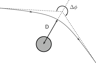
Figure 1: Definitions for unbounded orbits in the Schwarzschild background: minimal distance $D$ and deflection angle $\delta\phi\equiv\Delta\phi-\pi$.

In the following, we will refer to the initial condition $\vec{k}|_{P_{0}}\parallel\vec{\zeta}|_{P_{0}}$ as the “parallel case” and to the initial condition $\vec{k}|_{P_{0}}\perp\vec{\zeta}|_{P_{0}}$ as the “perpendicular case.” Three different initial conditions will be discussed explicitly. The first two are for the parallel case with either a $\oplus$– or a $\ominus$–mode. The third refers to the perpendicular case, but only for the $\oplus$–mode, as $~\widetilde{k}^{\mu}$ may be not well-defined for the $\ominus$–mode.

The constants of motion for the $\oplus$– and $\ominus$–modes coincide in the parallel case, so that both modes follow the same geodesic. This is not quite trivial, since the wave vector component $k^{0}$ differs for the two modes. For nonparallel $\vec{\zeta}|_{P_{0}}$ and $\vec{k}|_{P_{0}}$, the constants of motion do not coincide and the geodesics for the $\oplus$– and $\ominus$–mode with same initial momentum $\vec{k}|_{P_{0}}$ differ.

Specifically, the constants of motion for the parallel case, expressed in terms of the constants of motion for the standard photon, are

$$\epsilon\,\big{|}^{\text{\,parallel case}}_{\text{\,MCS}}=\sqrt{\frac{4E_{0}^{2}}{m^{2}}+1}$$ (4.11a)

and

$$\ell\,\big{|}^{\text{\,parallel case}}_{\text{\,MCS}}=\frac{2}{m}\,L_{0}\,,$$ (4.11b)

which hold for both $\oplus$– and $\ominus$–modes of MCS theory. For the perpendicular case, one finds

$$\epsilon\,\big{|}^{\text{\,perp. case}}_{\text{\,MCS $\oplus$}}=\sqrt{\frac{E_{0}^{2}}{m^{2}}+1}$$ (4.12a)

and

$$\ell\,\big{|}^{\text{\,perp. case}}_{\text{\,MCS $\oplus$}}=\frac{L_{0}}{m}\,,$$ (4.12b)

which hold for the $\oplus$–mode.

The “turning points” $D$ can also be compared. For MCS photons, $D$ is given by the largest root of the following cubic equation in $r$:

$$\frac{\ell^{2}}{r^{2}}-\frac{2GM\ell^{2}}{r^{3}}+1-\frac{2GM}{r}=\epsilon^{2},$$ (4.13)

while, for standard photons, one has to solve:

$$\frac{L_{0}^{2}}{r^{2}}-\frac{2GML_{0}^{2}}{r^{3}}=E_{0}^{2}\,.$$ (4.14)

The cubic (4.13) for parallel MCS $\oplus$– and $\ominus$–photons reduces to:

$$\frac{L_{0}^{2}}{r^{2}}-\frac{2GML_{0}^{2}}{r^{3}} =E_{0}^{2}+\frac{GMm^{2}}{2r}\,,$$ (4.15a)

and the one for perpendicular MCS $$\oplus$$–photons to:

$$\frac{L_{0}^{2}}{r^{2}}-\frac{2GML_{0}^{2}}{r^{3}} =E_{0}^{2}+\frac{2GMm^{2}}{r}\,.$$ (4.15b)

It is relatively easy to see by graphical methods that the turning point (distance of closest approach) $D$ is smaller for MCS photons than for standard photons with the same initial momentum. In addition, the turning points differ between the perpendicular and the parallel case: $D$ is smaller for the perpendicular case than for the parallel case.

Next, we calculate the deflection angle $\delta\phi$. It is explicitly given by

$$\delta\phi=2\int_{D}^{\infty}dr\medspace\frac{\ell}{r^{2}\sqrt{\epsilon^{2}-(1-2GM/r)(\ell^{2}/r^{2}+\chi)}}-\pi.$$ (4.16)

We, again, discuss the three cases just mentioned. A direct calculation with $\ell$ as independent variable turns out to be difficult. Instead, we take the turning point $D$ as independent variable. This means that we are comparing photons with the same distance of closest approach $D$, rather than having the same momentum or angular momentum.

The contributions to first order in $GM/D$ read for standard photons:

$$\delta\phi\Big{|}_{\text{\,standard}}\sim\frac{4GM}{D}\,,$$ (4.17a)

for parallel MCS $$\oplus \ominus$$– and –photons:

$$\delta\phi\Big{|}^{\text{\,parallel case}}_{\text{\,MCS}}\sim\frac{4GM}{D}\left(1+\frac{1}{8}\frac{m^{2}}{E_{0}^{2}}\right),$$ (4.17b)

and for perpendicular MCS $$\oplus$$–photons:

$$\delta\phi\Big{|}^{\text{\,perp. case}}_{\text{\,MCS}\,\oplus}\sim\frac{4GM}{D}\left(1+\frac{1}{2}\frac{m^{2}}{E_{0}^{2}}\right).$$ (4.17c)

These results show that the modifications are quadratic in the ratio of the Chern–Simons mass scale $m$ over the photon energy.

4.3 Deflection of light: general considerations

Because of the symmetries of the Schwarzschild metric, the spacetime coordinates can be chosen so that a geodesic is confined to the “equatorial plane,” $\theta=\pi/2$. But, the equatorial planes of a standard photon and an MCS photon, with same initial momentum $\vec{k}|_{P_{0}}$, need not coincide.

Now, choose particular asymptotic Minkowski coordinates, so that $\vec{k}$ is confined to the $x$–$y$ plane. The angle $\psi$ between the two equatorial planes is then determined by

$$\sin\psi=\widetilde{k}_{z}/|\,\vec{\widetilde{k}}\,|=\frac{{\alpha\,\zeta_{z}\,\left(\vec{k}\cdot\vec{\zeta}\,\right)}_{\vphantom{!_{a}}}}{{\sqrt{\left(1-\alpha\right)^{2}\left(\vec{k}\cdot\vec{k}-\left(\vec{k}\cdot\vec{\zeta}\,\right)^{2}\right)+\left(\vec{k}\cdot\vec{\zeta}\,\right)^{2}}}^{\vphantom{a}}}\;,$$ (4.18)

with $\alpha\equiv m^{2}/(2k^{\mu}k_{\mu})$.

The deflection of MCS light rays in a Schwarzschild background has, in general, two new contributions. First, the geodesic describing the path of light is timelike and, therefore, differs from the usual case. Second, the equatorial plane to which the geodesic is confined can be different from the usual case. This is because, as mentioned before, the wave vector $k^{\mu}$ does not generally point to the direction of propagation, which is determined by the modified wave vector $\widetilde{k}^{\mu}$ as defined by (3.7).

The equatorial planes of an MCS photon and a standard photon with same initial momentum $\vec{k}|_{P_{0}}$ do coincide for the parallel and perpendicular cases discussed in the previous subsection. The reason is that the component $\zeta_{z}$ in the numerator of Eq. (4.18) vanishes for the parallel case and that the inner product $\vec{k}\cdot\vec{\zeta}$ does so for the perpendicular case. For generic initial conditions, however, the angle between the two equatorial planes must be taken into account, in addition to the modification to the deflection angle by the timelike path.

4.4 Gravitational redshift

The modified geodesic equation also changes the gravitational redshift. Consider two static observers in a Schwarzschild background, i.e., two observers whose four-velocities $u_{1}^{\mu}$ and $u_{2}^{\mu}$ are tangent to the static Killing field $\xi^{\mu}$ of the Schwarzschild geometry. The frequency of a wave passing by, measured by a static observer at point $P_{i}$, reads then

$$\omega_{i}=k^{\mu}u_{\mu}|_{P_{i}}=k^{\mu}\xi_{\mu}\left(\xi^{\nu}\xi_{\nu}\right)^{-1/2}|_{P_{i}}=\left.k^{0}\,\sqrt{1-2GM/r}\;\right|_{P_{i}}\,.$$ (4.19)

For standard electromagnetic waves, the absolute and relative redshifts in a Schwarzschild geometry are given by [13]

$$\frac{\omega_{1}}{\omega_{2}} =\,\sqrt{\frac{1-2GM/r_{2}}{1-2GM/r_{1}}}$$ (4.20a)

and

$$\frac{\omega_{1}-\omega_{2}}{\omega_{1}} =\frac{GM}{r_{1}}-\frac{GM}{r_{2}}+\mathrm{O}\left(\left(GM/r_{\text{min}}\right)^{2}\right)\,,$$ (4.20b)

with $r_{\text{min}}\equiv\text{min}(r_{1},r_{2})$.

Assuming $\zeta^{a}e_{a}^{\;0}|_{P_{i}}=0$, the constant of motion (4.2a) for Maxwell–Chern–Simons waves of frequency (4.19) can be written as follows:

$$\epsilon=\left.\frac{2}{m}\left(1-\frac{m^{2}}{2k^{\mu}k_{\mu}}\right)\left(1-\frac{2GM}{r}\right)^{1/2}\,\omega_{i}\,\right|_{P_{i}}\,,$$ (4.21)

so that

$$\frac{\omega_{1}}{\omega_{2}}=\beta\;\;\sqrt{\frac{1-2GM/r_{2}}{1-2GM/r_{1}}}\;,$$ (4.22)

with

$$\beta\equiv\frac{{\left.\left(1-m^{2}/(2k^{\mu}k_{\mu})\right)\right|_{P_{2}}}_{\vphantom{!_{a}}}}{{\left.\left(1-m^{2}/(2k^{\nu}k_{\nu})\right)\right|_{P_{1}}}^{\vphantom{a}}}\,.$$ (4.23)

The relative redshift is then given by

$$\frac{\omega_{1}-\omega_{2}}{\omega_{1}}=\beta^{-1}\left(\frac{GM}{r_{1}}-\frac{GM}{r_{2}}\right)+1-\beta^{-1}+\mathrm{O}\left(\left(GM/r_{\text{min}}\right)^{2}\right).$$ (4.24)

In contrast to the results (4.17bc) for the deflection angle, the change of the redshift ($\beta\neq 1$) may be a linear effect in $m$, since it can be seen from (3.5) that the first contribution to $k^{\mu}k_{\mu}$ can be linear in $m$.

In order to evaluate $\beta$ explicitly, we have to specify the wave vector $k^{\mu}$ in relation to the parameter $\zeta^{\mu}$. For simplicity, we make two approximations.

First, assume that $\zeta^{\mu}k_{\mu}=0$ holds at the two points $P_{1}$ and $P_{2}$. In contrast to the previous discussion for the deflection of light, this is really an approximation, since this condition must hold at both points $P_{1}$ and $P_{2}\,$. Again, only the $\oplus$–mode will be discussed. Using the dispersion law (3.5), we find in the “perpendicular approximation”

$$\beta\;\Big{|}^{\text{\,perp. approx.}}_{\text{\,MCS}\;\oplus}=1\,,$$ (4.25)

which implies that the gravitational redshift (4.22) is not modified compared to the case of standard photons.

Second, assume that $\vec{k}$ is parallel to $\vec{\zeta}$ at the points $P_{1}$ and $P_{2}$. These three-vectors refer to the space components of $k^{\mu}$ and $\zeta^{\mu}$, respectively, in the coordinate system corresponding to the Schwarzschild line element (4.1). Concretely, one has

$$k^{j}|_{P_{i}}=\chi_{i}\,\zeta^{j}|_{P_{i}}\,,\quad\chi_{i}\neq 0\,,$$ (4.26)

for $i=1,2$ and $j=r,\theta,\phi$. Then, the following relation holds:

$$\left.k^{\mu}k_{\mu}\,\right|_{P_{i}}=\left.\pm\,\sqrt{m^{2}k^{0}k_{0}}\,\right|_{P_{i}}=\left.\pm\,m\,\omega_{\pm}\,\right|_{P_{i}}\,,$$ (4.27)

where the subscript ‘$+$’ on $\omega$ refers to the $\oplus$–mode and ‘$-$’ to the $\ominus$–mode. By inserting (4.27) into (4.22), we find

$$\frac{\omega_{\pm,1}\mp{m/2}}{\omega_{\pm,2}\mp m/2}=\sqrt{\frac{1-2GM/r_{2}}{1-2GM/r_{1}}}\,,$$ (4.28)

and the relative gravitational redshift becomes

$$\frac{\omega_{\pm,1}-\omega_{\pm,2}}{\omega_{\pm,1}}\Big{|}^{\text{\,parallel approx.}}_{\text{\,MCS}}=\left(1\mp\frac{m}{2\omega_{\pm,1}}\right)\;\Delta_{\text{standard}}^{\text{(Schw.)}}\equiv y\;\Delta_{\text{standard}}^{\text{(Schw.)}}\,,$$ (4.29)

in terms of the relative gravitational redshift of standard photons in a Schwarzschild background,

$$\Delta_{\text{standard}}^{\text{(Schw.)}}\equiv\frac{{\sqrt{1-2GM/r_{2}}-\sqrt{1-2GM/r_{1}}}_{\vphantom{!_{a}}}}{{\sqrt{1-2GM/r_{2}}}^{\vphantom{a}}}\,.$$ (4.30)

Apparently, the redshifts of $\oplus$– and $\ominus$–modes differ in this approximation. With $m>0$, the redshift for a parallel $\ominus$–photon is larger than for a standard photon and the redshift for a parallel $\oplus$–photon smaller. The effect is significant for frequencies of order $m$, but tends to zero for higher frequencies. The modified redshifts in the parallel approximation are shown in Fig. 2.

The parallel approximation is a nontrivial restriction and, strictly speaking, may only be applicable for sufficiently short geodesic segments. Still, we conjecture that the splitting up of the two MCS photon modes is a general phenomenon. The redshift results for a Robertson–Walker universe (see Appendix A) indeed suggest that the effect appears in general curved spacetime backgrounds and is not confined to the Schwarzschild background.

Figure 2: Modification of the gravitational redshift for two polarization modes of Maxwell–Chern–Simons photons in the parallel approximation (4.26). The relative redshift $\displaystyle{(\omega_{\pm,1}-\omega_{\pm,2})/\omega_{\pm,1}}$ from Eq. (4.29), divided by the relative redshift for standard photons, is denoted $y$ and the normalized frequency $x\equiv\displaystyle{\omega_{\pm,1}/m}$. For the “massive” $\oplus$–mode, the norm $k^{\mu}k_{\mu}=\omega^{2}-|\vec{k}|^{2}$ is equal to or larger than $m^{2}$, so that $x\geq 1$.

5 Conclusion

The main topic of the present article has been the coupling of Maxwell–Chern–Simons theory to gravity. But, treating the gravitational field dynamically leads to incompatibilities between the field equations and the spacetime geometry [12]. Therefore, we have only been able to consider the gravitational effects from a fixed spacetime background, as described by the action (2.7).

Using the approximation of geometrical optics, we have found new phenomena for the propagation of Maxwell–Chern–Simons waves in a given gravitational background. In particular, it was observed that the wave vector $k^{\mu}$ no longer obeys a geodesic equation. A modified wave vector $\widetilde{k}^{\mu}$ can, however, be defined, which is tangent to timelike geodesics; see Eqs. (3.7) and (3.8). In the flat limit, $\widetilde{k}^{\mu}$ corresponds to the group velocity and the interpretation is that generally these timelike geodesics describe the “light rays” of Maxwell–Chern–Simons theory.

The timelike geodesics allow for having light rays in stable bounded orbits around a nonrotating, spherically symmetric mass distribution, as described by the static Schwarzschild metric. Also, the parameters for unbounded orbits in a Schwarzschild background and the corresponding redshifts were discussed in some detail.

It is noteworthy that, in spite of the fundamental inconsistencies which occur for coupling Maxwell–Chern–Simons theory to gravity, the light rays are found to be simple geodesics. The results of Refs. [1, 3] suggest that Maxwell–Chern–Simons theory (2.7) with a spacelike fourvector $\zeta^{\mu}$ preserves causality. The fact that the geodesics found are timelike further supports this suggestion. For timelike fourvector $\zeta^{\mu}$, on the other hand, we find that light would follow spacelike geodesics, which would, again, indicate that Maxwell–Chern–Simons theory with a timelike parameter $\zeta^{\mu}$ violates causality.

The effects discussed in this article (e.g., stable bounded orbits and modified redshifts) are significant for wave frequencies of the order of the Chern–Simons parameter $m$. If the model considered applies directly to the photon, the astronomical bounds on $m$ in the present universe are very tight [1, 2], $m\lesssim 10^{-33}\,\mathrm{eV}$, and the results of the present article are, most likely, unobservable. But, for a Chern–Simons term arising from a nontrivial spacetime structure or from a quantum phase transition of a fermionic quantum vacuum, it is possible to imagine circumstances where $m$ is no longer extremely small and the effects discussed may perhaps become observable.

Appendix A Redshift in a Robertson–Walker universe

In this appendix, we consider the redshift of Maxwell–Chern–Simons (MCS) photons in a Robertson–Walker (RW) universe. The line element is given by [13]

$$ds^{2}=dt^{2}-a^{2}(t)\,d\Omega^{2},$$ (A.1)

with scale factor $a(t)$ and

$$d\Omega^{2}\equiv\begin{cases}d\psi^{2}+\sin^{2}\psi\left(d\theta^{2}+\sin^{2}\theta d\phi^{2}\right)\,,\\ dx^{2}+dy^{2}+dz^{2}\,,\\ d\psi^{2}+\sinh^{2}\psi\left(d\theta^{2}+\sin^{2}\theta d\phi^{2}\right)\,,\end{cases}$$ (A.2)

for positive, zero, and negative curvature, respectively.

In order to justify the treatment of the redshift as a background problem, we could take a closed, matter-dominated Robertson–Walker universe of positive curvature, with $\rho$ the matter density of the universe and $\rho\,a^{3}$ constant [13]. The MCS parameter $m$ should then be small compared to the rest mass of the universe, $m\ll\rho\,a^{3}$, so that a typical photon energy $m$ can be neglected compared to the energy content of the matter. Purely mathematically, however, the results of this appendix apply to any Robertson–Walker background metric.

The redshift of a “standard” photon in a Robertson–Walker universe is [13]

$$\frac{\omega_{2}}{\omega_{1}}=\frac{a(t_{1})}{a(t_{2})}\,,$$ (A.3)

and the relative redshift reads

$$\Delta_{\text{standard}}^{\text{(RW)}}\equiv\frac{\omega_{1}-\omega_{2}}{\omega_{1}}=1-\frac{a(t_{1})}{a(t_{2})}\,.$$ (A.4)

For an MCS photon, we assume $\zeta^{\mu}u_{\mu}=0$, where $u_{\mu}$ is the four velocity of a comoving observer and $\zeta^{a}=\zeta^{\mu}e_{\mu}^{\;a}$ is the parameter of the action (2.7). The following expression for the gravitational redshift of MCS photons is then found:

$$\frac{{\left.\left[\,\big{(}\left[1-m^{2}/2k^{\mu}k_{\mu}\right]\,\omega\big{)}^{2}-m^{2}/4\,\right]^{1/2}\,\right|_{P_{2}}}_{\vphantom{!_{a}}}}{{\left.\left[\,\big{(}\left[1-m^{2}/2k^{\nu}k_{\nu}\right]\,\omega\big{)}^{2}-m^{2}/4\,\right]^{1/2}\,\right|_{P_{1}}}^{\vphantom{a}}}=\frac{a(t_{1})}{a(t_{2})}\,.$$ (A.5)

To evaluate (A.5), we use the same approximations as in Section 4.4. Assuming $\zeta^{\mu}k_{\mu}=0$ at the points $P_{1}$ and $P_{2}$ leads to

$$\frac{\omega_{2}}{\omega_{1}}\Big{|}^{\text{\,perp. approx.}}_{\text{\,MCS}\;\oplus}=\frac{a(t_{1})}{a(t_{2})}\left[1+m^{2}\left(\frac{1}{\omega_{2}^{2}}-\frac{1}{\omega_{1}^{2}}\right)+\mathrm{O}\left(\left(\frac{m}{\omega_{\text{min}}}\right)^{4}\,\right)\right],$$ (A.6)

where we have expanded in $m/\omega_{i}$ and defined $\omega_{\text{min}}\equiv\min(\omega_{1},\omega_{2})$. Again, this expression is only valid for the $\oplus$–mode. The parallel approximation $\vec{\zeta}\parallel\vec{k}$ gives for the $\oplus$–mode:

$$\frac{\omega_{2}}{\omega_{1}}\Big{|}_{\,\text{MCS}\;\oplus}^{\,\text{parallel approx.}}= \frac{a(t_{1})}{a(t_{2})}\left[1+m\left(\frac{1}{2\omega_{2}}-\frac{1}{2\omega_{1}}\right)\right.$$ (A.7)

$$+\left.m^{2}\left(\frac{3}{8\omega_{2}^{2}}-\frac{1}{4\omega_{1}\omega_{2}}-\frac{1}{8\omega_{1}^{2}}\right)+\mathrm{O}\left(\left(\frac{m}{\omega_{\text{min}}}\right)^{3}\,\right)\right],$$

and for the $\ominus$–mode:

$$\frac{\omega_{2}}{\omega_{1}}\Big{|}^{\text{\,parallel approx.}}_{\,\text{MCS}\;\ominus}= \frac{a(t_{1})}{a(t_{2})}\left[1-m\left(\frac{1}{2\omega_{2}}-\frac{1}{2\omega_{1}}\right)\right.$$ (A.8)

$$+\left.m^{2}\left(\frac{3}{8\omega_{2}^{2}}-\frac{1}{4\omega_{1}\omega_{2}}-\frac{1}{8\omega_{1}^{2}}\right)+\mathrm{O}\left(\left(\frac{m}{\omega_{\text{min}}}\right)^{3}\,\right)\right].$$

To leading order in $m$, the relative redshifts then read

$$\frac{\omega_{1}-\omega_{2}}{\omega_{1}}\Big{|}_{\,\text{MCS}\;\oplus}^{\,\text{perp approx.}}\hskip 8.99994pt \sim \;\left(1-\frac{m^{2}}{\omega_{1}^{2}}\;\frac{a(t_{1})+a(t_{2})}{a(t_{1})}\right)\Delta_{\text{standard}}^{\text{(RW)}}\,,$$ (A.9a)

$$\frac{\omega_{1}-\omega_{2}}{\omega_{1}}\Big{|}_{\,\text{MCS}\;\oplus}^{\,\text{parallel approx.}} \sim \;\left(1-\frac{m}{2\omega_{1}}\right)\Delta_{\text{standard}}^{\text{(RW)}}\,,$$ (A.9b)

$$\frac{\omega_{1}-\omega_{2}}{\omega_{1}}\Big{|}_{\,\text{MCS}\;\ominus}^{\,\text{parallel approx.}} \sim \;\left(1+\frac{m}{2\omega_{1}}\right)\Delta_{\text{standard}}^{\text{(RW)}}\,,$$ (A.9c)

in terms of the standard result (A.4).

Already in the perpendicular approximation, $k^{\mu}\zeta_{\mu}=0$, we find a nonvanishing effect, in contrast to the Schwarzschild case with Eqs.  (4.22) and (4.25). The modification is, however, only of order $m^{2}$, according to Eq. (A.6). In an expanding universe with $a(t_{2})>a(t_{1})$ for $t_{2}>t_{1}$, the redshift (A.9a) for the perpendicular $\oplus$–mode is smaller than for a standard photon.

In the parallel approximation, we find, to leading order in $m$, the same result as for the Schwarzschild case with Eq. (4.29). The redshift splits up between the two modes: with $m>0$, the redshift (A.9b) of a parallel $\oplus$–mode in an expanding universe is smaller than the one of a standard photon, while the redshift (A.9c) of a parallel $\ominus$–mode is larger.

Appendix E Erratum [Nucl. Phys. B 809 (2009) 362]

In a previous article [16], we have discussed gravitational effects in Maxwell–Chern–Simons (MCS) theory [1], whose action has a bilinear Chern–Simons (CS) term added to the standard Maxwell term. In particular, we considered MCS light propagation in fixed Schwarzschild and Robertson–Walker spacetime backgrounds, described by a quartic dispersion relation

$$\left(k_{\mu}k^{\mu}\right)^{2}+m^{2}\,k_{\mu}k^{\mu}\,\zeta_{\nu}\zeta^{\nu}-m^{2}\left(\zeta_{\mu}k^{\mu}\right)^{2}=0\,,$$ (E.1)

where $k_{\mu}\equiv(\omega/c,\vec{k})$ is the wave number four-vector, $m$ the CS mass scale, and $\zeta_{\mu}=\zeta_{\mu}(x)$ the spacelike CS “four-vector.” The geometrical-optics approximation of this theory was considered and a modified wave number four-vector $\widetilde{k}^{\mu}$ was introduced. It was claimed, in Section 3 of Ref. [16], that this $\widetilde{k}^{\mu}$ obeys a geodesic-like equation. However, we have now realized that this statement is incorrect.

Instead of Eq. (3.9) of Ref. [16], the complete equation for $\widetilde{k}^{\mu}$ reads:

$$\widetilde{k}^{\mu}D_{\mu}\widetilde{k}_{\lambda}=m^{4}/(4\,k^{4})\left(2\,k_{\lambda}\,\zeta^{\rho}\,k_{\rho}/k^{2}-\zeta_{\lambda}\right)\,k^{\mu}k^{\nu}\,D_{\mu}\zeta_{\nu}\,,$$ (E.2)

with $k^{2}\equiv k^{\mu}k_{\mu}=g_{\mu\nu}\,k^{\mu}k^{\nu}$. In general, the right-hand side of (E.2) does not vanish and (E.2) is not a geodesic-like equation.

Studies of different concrete examples have shown that the results of our article are, in general, invalid, despite of the fact that (E.1) implies that $k^{\mu}k_{\mu}$ is of order $m\omega$ and that the right-hand side of (E.2) is, therefore, suppressed by a factor of order $m^{2}/\omega^{2}$. However, some qualitative and quantitative results of Ref. [16] remain valid for special CS parameters $\zeta_{\mu}(x)$.

Consider, first, the case of a Schwarzschild spacetime background, as discussed in Section 4 of Ref. [16]. For the following choice of CS parameters

$$\left(\zeta_{t},\,\zeta_{r},\,\zeta_{\theta},\,\zeta_{\phi}\,\right)=\left(0,\,\pi/2-\theta,\,-r,\,0\,\right),$$ (E.3)

an explicit solution for the modified wavevector $\widetilde{k}_{\mu}$ can be found, corresponding to the perpendicular $\oplus$–modes as discussed in Sections 4.1 and 4.2 of Ref. [16]. The results for the deflection angles and the discussion concerning the closed orbits remain valid, but, in contrast to the claim in our article, these orbits become unstable, because they depend sensitively on the initial conditions. If $\widetilde{k}_{\mu}$ does not lie entirely in the equatorial plane, the geodesic equation acquires a correction term and a simple treatment is no longer valid.

The Schwarzschild gravitational redshift with parameters (E.3) does not differ from the redshift for standard Lorentz-invariant photons. This result is consistent with Eq. (4.25) of Ref. [16], since the solution is a perpendicular $\oplus$–mode. More complicated and nonperpendicular examples also show no modification compared to the standard redshift, in disagreement with the discussion in Section 4.4 in Ref. [16].

Consider, next, the case of a spatially-flat Robertson–Walker spacetime background with line element

$$ds^{2}=dt^{2}-a^{2}(t)\left(dx^{2}+dy^{2}+dz^{2}\right),$$ (E.4)

as discussed in Appendix A of Ref. [16]. But, now, there is the additional condition that the nonnegative scale factor $a(t)$ is bounded from above, so that the metric considered does not completely describe an expanding flat Friedmann–Robertson–Walker universe [which has $a(t)\to\infty$ for $t\to\infty$].

For the following choice of CS parameters $\zeta_{\mu}(t)$ with constant $\zeta_{3}\neq 0$

$$\zeta_{\mu}(t)=\left(\,\sqrt{-1+\zeta_{3}^{2}/{a^{2}(t)}},\,0,\,0,\,\zeta_{3}\,\right),$$ (E.5)

the splitting of the two modes persists qualitatively, but must be corrected quantitatively compared to what is given in Ref. [16]. Remark that (E.5) is, up to coordinate transformations, the only choice of CS parameters, which fulfills the conditions

$$\zeta_{\mu}\zeta^{\mu}=-1,\quad D_{\lambda}\,\zeta_{\mu}-D_{\mu}\,\zeta_{\lambda}=0.$$ (E.6)

But (E.5) is obviously only defined for $a(t)<\left|\zeta_{3}\right|$. The particular choice of CS parameters (E.5) violates Lorentz and diffeomorphism invariance. These violations lead to inconsistencies, when MCS–theory is coupled to gravity. A minimal coupling procedure gives rise to a nonconserved, nonsymmetric energy-momentum tensor, which is incompatible with the Bianchi identities [12]. As in our original publication [16], gravity is not treated dynamically in this Erratum but is considered as a background for the propagation of light described by dispersion relation (E.1).

The redshift (or blueshift) behavior of the $\oplus$ and $\ominus$ polarization modes in a Robertson–Walker spacetime background with line element (E.4) is, to first order in $m/\omega$, given by the following expressions:

$$\frac{\omega_{1\;\oplus}}{\omega_{2\;\oplus}} = \frac{a(t_{2})}{a(t_{1})}\,\left(1-\frac{m}{2}\;\frac{\zeta_{0}(t_{1})\,a(t_{1})-\zeta_{0}(t_{2})\,a(t_{2})}{|\vec{k}|}\right)+\mathrm{O}\left(m^{2}/|\vec{k}|^{2}\right),$$ (E.7a)

$$\frac{\omega_{1\;\ominus}}{\omega_{2\;\ominus}} = \frac{a(t_{2})}{a(t_{1})}\,\left(1+\frac{m}{2}\;\frac{\zeta_{0}(t_{1})\,a(t_{1})-\zeta_{0}(t_{2})\,a(t_{2})}{|\vec{k}|}\right)+\mathrm{O}\left(m^{2}/|\vec{k}|^{2}\right),$$ (E.7b)

with $\zeta_{0}(t)$ defined by the first component on the right-hand side of (E.5). Most interestingly, the Robertson–Walker gravitational redshift is different for the two MCS polarization modes, already at the first order in $m/\omega$.

For the benefit of the reader, we now list the problematic equations of our original article. The following general equations of Ref. [16] are incorrect as they stand: (3.9), (4.18), and (A.5), together with all equations referring to the so-called parallel case. As mentioned above, Eq. (3.9) of Ref. [16] is replaced by (E.2) of the present Erratum. The following equations of Section 4 in Ref. [16] do not hold in general but do hold for the special parameters (E.3) of this Erratum: (4.2)–(4.10), (4.12)–(4.14), (4.15b), (4.16), (4.17c), (4.21)–(4.25). Finally, Eqs. (A6)–(A8) of Ref. [16] are replaced by the results (E.7ab) for the special parameters (E.5) of this Erratum, where the new results hold for wave vectors $\vec{k}$ with arbitrary directions.

References

- [1] S.M. Carroll, G.B. Field, and R. Jackiw, Limits on a Lorentz- and parity-violating modification of electrodynamics, Phys. Rev. D 41 (1990) 1231.
- [2] D. Colladay and V.A. Kostelecký, Lorentz-violating extension of the standard model, Phys. Rev. D 58 (1998) 116002, hep-ph/9809521.
- [3] C. Adam and F.R. Klinkhamer, Causality and CPT violation from an Abelian Chern-Simons-like term, Nucl. Phys. B 607 (2001) 247, hep-ph/0101087.
- [4] C. Adam and F.R. Klinkhamer, Photon decay in a CPT-violating extension of quantum electrodynamics, Nucl. Phys. B 657 (2003) 214, hep-th/0212028.
- [5] C. Kaufhold and F.R. Klinkhamer, Vacuum Cherenkov radiation and photon triple-splitting in a Lorentz-noninvariant extension of quantum electrodynamics, hep-th/0508074.
- [6] F.R. Klinkhamer, A CPT anomaly, Nucl. Phys. B 578 (2000) 277, hep-th/9912169.
- [7] F.R. Klinkhamer and J. Schimmel, CPT anomaly: a rigorous result in four dimensions, Nucl. Phys. B 639 (2002) 241, hep-th/0205038.
- [8] F.R. Klinkhamer, Fundamental time-asymmetry from nontrivial space topology, Phys. Rev. D 66 (2002) 047701, gr-qc/0111090.
- [9] F.R. Klinkhamer and G.E. Volovik, Quantum phase transition for the BCS–BEC crossover in condensed matter physics and for CPT violation in elementary particle physics, JETP Lett. 80 (2004) 343, cond-mat/0407597.
- [10] F.R. Klinkhamer and G.E. Volovik, Emergent CPT violation from the splitting of Fermi points, Int. J. Mod. Phys. A 20 (2005) 2795, hep-th/0403037.
- [11] V. Gurarie, L. Radzihovsky, and A.V. Andreev, Quantum phase transitions across a –wave Feshbach resonance, Phys. Rev. Lett. 94 (2005) 230403, cond-mat/0410620.
- [12] V.A. Kostelecký, Gravity, Lorentz violation and the standard model, Phys. Rev. D 69 (2004) 105009, hep-th/0312310.
- [13] R.M. Wald, General Relativity, University of Chicago Press, Chicago, 1984.
- [14] M. Born and E. Wolf, Principles of Optics, 7th ed., Cambridge University Press, Cambridge, 1999.
- [15] L. Brillouin, Wave Propagation and Group Velocity, Academic, New York, 1960.
- [16] E. Kant, F.R. Klinkhamer, Maxwell–Chern–Simons theory for curved spacetime backgrounds, Nucl. Phys. B 731 (2005) 125, arXiv:hep-th/0507162v4.