hep-th/0507153

ZMP-HH/05-16

The effective action of type II Calabi-Yau orientifolds

Thomas W. Grimm

II. Institut für Theoretische Physik
Universität Hamburg, Luruper Chaussee 149
D-22761 Hamburg, Germany
and Zentrum für Mathematische Physik
Universität Hamburg, Bundesstrasse 55
D-20146 Hamburg, Germany

thomas.grimm@desy.de

ABSTRACT

This article first reviews the calculation of the $N=1$ effective action for generic type IIA and type IIB Calabi-Yau orientifolds in the presence of background fluxes by using a Kaluza-Klein reduction. The Kähler potential, the gauge kinetic functions and the flux-induced superpotential are determined in terms of geometrical data of the Calabi-Yau orientifold and the background fluxes. As a new result, it is shown that the chiral description directly relates to Hitchin’s generalized geometry encoded by special odd and even forms on a threefold, whereas a dual formulation with several linear multiplets makes contact to the underlying $N=2$ special geometry. In type IIB setups, the flux-potentials can be expressed in terms of superpotentials, D-terms and, generically, a massive linear multiplet. The type IIA superpotential depends on all geometric moduli of the theory. It is reviewed, how type IIA orientifolds arise as a special limit of M-theory compactified on specific $G_{2}$ manifolds by matching the effective actions. In a similar spirit type IIB orientifolds are shown to descend from F-theory on a specific class of Calabi-Yau fourfolds. In addition, mirror symmetry for Calabi-Yau orientifolds is briefly discussed and it is shown that the $N=1$ chiral coordinates linearize the appropriate instanton actions.

Acknowledgments

This article is based on my Ph.D. thesis. First of all I would like to express my deep gratitude to my supervisor Prof. Jan Louis for his continuous support, expert advises and encouragement. The collaboration with Mariana Graña, Hans Jockers, Frederic Schuller and Mattias Wohlfarth was very enjoyable and fruitful. I esspecially like to thank my office mates Iman Benmachiche, Olaf Hohm, Hans Jockers, Andrei Micu and Anke Knauf for providing a very delighting athmosphere and the numerous discussions about physiscs and beyond. I am also indebted to David Cerdeño, Vincente Cortés, Frederik Denef, Sergei Gukov, Henning Samtleben, Sakura Schäfer-Nameki, Shamit Kachru, Boris Körs, Paolo Merlatti, Thorsten Prüstel, Waldemar Schulgin, Silvia Vaulà and Martin Weidner for various discussions and correspondence. I am grateful to my lovely girlfriend, for supporting me through the last years.

This work is supported by the DFG – The German Science Foundation, the DAAD – the German Academic Exchange Service, and the European RTN Program MRTN-CT-2004-503369.

Chapter 1 Introduction

The Standard Model of particle physics extended by massive neutrinos has been tested to a very high precision and is believed to correctly describe the known elementary particles and their interactions. Experimentally, the only missing ingredient is the scalar Higgs particle, which gives masses to the leptons and quarks, once it acquires a vacuum expectation value. The Standard Model provides a realistic model of a renormalizable gauge theory. Despite its impressive success there are also various theoretical drawbacks, such as the large number of free parameters, the hierarchy and naturalness problem as well as the missing unification with gravity. These indicate that it cannot be viewed as a fundamental theory, but rather should arise as an effective description.

A natural extension of the Standard Model is provided by supersymmetry, which serves as a fundamental symmetry between bosons and fermions. Supersymmetry predicts a superpartner for all known particles and thus basically doubles the particle content of the theory. However, none of the superpartners was ever detected in an accelerator experiment, which implies that supersymmetry is appearing in its broken phase. The supersymmetric Standard Model solves some of the problems of the Standard Model [1]. Even in its (softly) broken phase it forbids large quantum corrections to scalar masses. This allows the Higgs mass to remain to be of order the weak scale also in a theory with a higher mass scale. Furthermore, assuming the supersymmetric Standard Model to be valid up to very high scales, the renormalization group flow predicts a unification of all three gauge-couplings. This supports the idea of an underlying theory relevant beyond the Standard Model scales. However, it remains to unify these extensions with gravity.

On the other hand, we know that General Relativity links the geometry of spacetime with the distribution of the matter densities. Einsteins theory is very different in nature. It is a classical theory which is hard to quantize due to its ultra-violet divergences (see however [2]). This fact constraints its range of validity to phenomena, where quantum effects are of negligible importance. However, there is no experimental evidence which contradicts large scale predictions based on General Relativity.

Facing these facts General Relativity and the Standard Model seems to be incompatible, in the sense that neither of them allows to naturally adapt the other. This becomes important in regimes where both theories have to be applied in order to describe the correct physics. Early time cosmology or physics of black holes are only two regimes where the interplay of quantum and gravitational effects become important. To nevertheless approach this theoretically interesting questions one might hope for a fundamental quantum theory combining the Standard Model and General Relativity. Until now one does not know what this unifying theory is, but one has at least one possible candidate. This theory is known as String Theory, which was studied intensively from various directions in the last thirty years. A comprehensive introduction to the subject can be found in [3, 4, 5].

Perturbative String Theory is a quantum theory of one-dimensional extended objects which replace the ordinary point particles. These fundamental strings can appear in various vibrational modes which at low energies are identified with different particles. The characteristic length of the string is $\sqrt{\alpha^{\prime}}$, where $\alpha^{\prime}$ is the Regge slope. Hence, the extended nature of the strings only becomes apparent close to the string scale $1/\sqrt{\alpha^{\prime}}$. The string spectrum naturally includes a mode corresponding to the graviton. This implies that Sting Theory indeed includes gravity and as we will further discuss below reduces to Einsteins theory at low energies. It most likely provides a renormalizable quantum theory of gravity around a given background. It avoids the ultra-violet divergences of graviton scattering amplitudes in field theory by smearing out the location of the interactions.

The extended nature of the fundamental strings poses strong consistency constraints on the theory. Non-tachyonic String Theories (Superstring Theories) require space-time supersymmetry and predict a ten-dimensional space-time at weak coupling. Altogether there are only five consistent String Theories, which are called type IIA, type IIB, heterotic $SO(32)$ and $E_{8}\times E_{8}$ and type I. These theories are connected by various dualities and one may eventually hope to unify all of them into one fundamental theory [6, 4].

As striking a proper formulation of such a fundamental theory might be, much of its uniqueness and beauty could be spoiled in attempting to extract four-dimensional results. This is equally true for the five String Theories formulated in ten dimensions. One approach to reduce String Theory from ten to four space-time dimensions is compactification on a geometric background of the form ${\mathbb{M}^{3,1}}\times{Y}$. ${\mathbb{M}^{3,1}}$ is identified with our four-dimensional world, while ${Y}$ is chosen to be small and compact, such that these six additional dimensions are not visible in experiments. This however induces a high amount of ambiguity, since String Theory allows for various consistent choices of ${Y}$. Eventually one would hope to find a String Field Theory formulated in ten dimensions, which resolves this ambiguity and dynamically chooses a certain background. However, such a theory is still lacking and one is forced to take a sideway to find and explore consistent string backgrounds.

For a given background, the ten-dimensional theory can then be reduced to four dimensions by a Kaluza-Klein compactification [7] (for a review on Kaluza-Klein reduction see e.g. [8]). This amounts to expanding the fields into modes of ${Y}$ and results in a full tower of Kaluza-Klein modes for each of the string excitations. Additionally there are winding modes corresponding to strings winding around cycles in ${Y}$. Generically it is hard and phenomenologically not interesting to deal with these infinite towers of modes and an effective description is needed.

In order to extract an effective formulation one may first integrate out the massive string excitations with masses of order $1/\sqrt{\alpha^{\prime}}$. This is possible due to the fact that the string scale $1/\sqrt{\alpha^{\prime}}$ is usually set to be of order the Planck scale such that gravity couples with Newtonian strength. In the point-particle limit $\alpha^{\prime}\rightarrow 0$ the effective theory describing the massless string modes is a supergravity theory (see e.g. [3, 4]). It can be constructed by calculating string scattering amplitudes for massless states. One then infers an effective action for these fields encoding the same tree level scattering vertices. An example is the three-graviton scattering amplitude in String Theory, which in an effective description can be equivalently obtained from the ten-dimensional Einstein-Hilbert term. Repeating the same reasoning for all other massless string modes yields a ten-dimensional supergravity theory for each of the five String Theories.

In a similar spirit one can also extract an effective Kaluza-Klein theory. For a compact internal manifold ${Y}$ the first massive Kaluza-Klein modes have a mass of order $1/R$, where $R$ is the ‘average radius’ of ${Y}$. Hence, choosing ${Y}$ to be sufficiently small these modes become heavy and can be integrated out. On the other hand, ${Y}$ has to be large enough that winding modes of length $\sqrt{\alpha^{\prime}}$ can be discarded. Together for $p$ being the characteristic momentum of the lower-dimensional fields an effective description of the massless modes is valid in the regime $1/p\gg R\gtrsim\sqrt{\alpha^{\prime}}$.

The structure of the four-dimensional theory obtained by such a reduction highly depends on the chosen internal manifold. The properties of ${Y}$ determine the amount of supersymmetry and the gauge-groups of the lower-dimensional theory. Generically one insists that ${Y}$ preserves some of the ten-dimensional supersymmetries. This is due to the fact that string theory on supersymmetric backgrounds is under much better control and various consistency conditions are automatically satisfied. It turns out that looking for a supersymmetric theory with a four-dimensional Minkowski background the internal manifold has to be a Calabi-Yau manifold [9]. From a phenomenological point of view the resulting low-energy supergravity theories need to include gauged matter fields filling the spectrum of the desired gauge theory such as the supersymmetric Standard Model. However, parameters like the size and shape of the compact space appear as massless neutral scalar fields in four dimensions. They label the continuous degeneracy of consistent backgrounds ${Y}$ and are generically not driven to any particular value; they are moduli of the theory. In a Standard Model-like vacuum these moduli have to be massive, such that they are not dynamical in the low-energy effective action. Therefore one needs to identify a mechanism in String Theory which induces a potential for these scalars. As it is well-known for supergravity theories this potential can provide at the same time a way to spontaneously break supersymmetry.

To generate a moduli-dependent potential in a consisted String Theory setup is a non-trivial task and requires further refinements of the standard compactifications. Recently, much effort was made to establish controllable mechanisms to stabilize moduli fields in type II String Theory. The three most popular approaches are the inclusion of background fluxes [10]–[41], instanton corrections [42, 43, 44, 45] and gaugino condensates [46, 44]. This raised the hope to find examples of string vacua with all moduli being fixed [35, 40, 41, 47]. Moreover, phenomenologically interesting scenarios for particle physics and cosmology can be constructed within these setups [48, 49].

In contrast to $E_{8}\times E_{8}$ and $SO(32)$ heterotic String Theory and type I strings both Type II String Theory do not consist of non-Abelian gauge-groups in their original formulation. Thus most of the model building was first concentrated on the heterotic String Theory as well as type I strings. This has changed after the event of the D-branes [50, 4, 51, 52], which naturally induce non-trivial gauge theories. It turned out that compactifications with space-time filling D-branes combined with moduli potentials due to fluxes or non-perturbative effects provide a rich arena for model building in particle physics as well as cosmology [48, 49]. One of the reasons is that consistent setups with D-branes and fluxes generically demand a generalization of the Kaluza-Klein Ansatz to so-called warped compactifications [12, 14, 19, 20]. Remarkably, these compactifications provide a String Theory realization of models with large hierarchies [14, 16, 18, 19, 20] as they were first suggested in [53].

One of the major motivation of this work it to analyze the low energy dynamics of the (bulk) supergravity moduli fields within a brane world setup with a non-vanishing potential. Hence, we will more carefully introduce the basic constituents in the following.

1.1 Compactification and moduli stabilization

Sting Theory is consistently formulated in a ten-dimensional space-time. In order in order to make contact with our four-dimensional observed world one is forced to assign six of these dimensions to an invisible sector. This can be achieve by choosing these dimensions to be small and compact and not detectable in present experiments. Even though the additional dimensions are not observed directly, they influence the resulting four-dimensional physics in a crucial way.

The idea of geometric compactification is rather old and goes back to the work of Kaluza and Klein in 1920 considering compactification of five-dimensional gravity on a circle [7]. They aimed at combining gravity with $U(1)$ gauge theory in a higher-dimensional theory. Through our motivations have changed, the techniques are very similar and can be generalized to the reduction from ten to four dimensions.

In the Kaluza-Klein reduction one starts by specifying an Ansatz for the background space-time [8]. Topologically it is assumed to be a manifold of the product structure

$$\mathcal{M}_{10}={\mathbb{M}^{3,1}}\times{Y}\ ,$$ (1.1)

where ${\mathbb{M}^{3,1}}$ represent the four observed non-compact dimensions and ${Y}$ correspond to the compact internal manifold. On this space one specifies a block-diagonal background metric

$$ds^{2}=g^{(4)}_{\mu\nu}(x)\,dx^{\mu}dx^{\nu}+g^{(6)}_{mn}(y)\,dy^{m}dy^{n}$$ (1.2)

where $g^{(4)}_{\mu\nu}$ is a four-dimensional Minkowski metric and $g^{(6)}_{ab}$ is the metric on the compact internal subspace. More generally, one can include a nontrivial warp factor $e^{2A(y)}$ depending on the internal coordinates $y$ into the Ansatz (1.2). This amounts to replacing $g^{(4)}_{\mu\nu}(x)$ with $e^{2A(y)}g^{(4)}_{\mu\nu}(x)$ which is the most general Ansatz for a Poincaré invariant four-dimensional metric [54, 10, 12, 14, 19, 20]. The functional form of the warp factor is then determined by demanding the background Ansatz to be a solution of the supergravity theory. It becomes a non-trivial function in the presence of localized sources such as D-branes. However, for simplicity we will restrict ourselves to the Ansatz (1.2) in the following.

The lower-dimensional theory is obtained by expanding all fields into modes of the internal manifold ${Y}$. As an illustrative example we discuss the Kaluza-Klein reduction of a ten-dimensional scalar $\Phi(x,y)$ fulfilling the ten-dimensional Laplace equation $\Delta_{10}\Phi=0$ [8]. Using the Ansatz (1.2) the Laplace operator splits as $\Delta_{10}=\Delta_{4}+\Delta_{6}$ and we may apply the fact that $\Delta_{6}$ on a compact space has a discrete spectrum. The coefficients arising in the expansion of $\Phi(x,y)$ into eigenfunctions of $\Delta_{6}$ are fields depending only on the coordinates of ${\mathbb{M}^{3,1}}$. From a four dimensional point of view the term $\Delta_{6}\Phi$ thus appears as a mass term. One ends up with an infinite tower of massive states with masses quantized in terms of $1/R$, where $R$ is the ‘radius’ of ${Y}$ such that $\text{Vol}({Y})$ is of order $R^{6}$. Choosing the internal manifold to be small enough the massive Kaluza-Klein states become heavy and can be integrate out. The resulting effective theory encodes the dynamics of the four-dimensional fields associated with the massless Kaluza-Klein modes satisfying

$$\Delta_{6}\Phi(x,y)\ =\ 0\ .$$ (1.3)

In chapter 2 we review how this procedure can be generalized to all other fields present in the ten-dimensional supergravity theories. This also includes the metric itself [8]. Equation (1.2) specifies the ten-dimensional background metric and a gravity theory describes variations around this Ansatz. In the non-compact dimensions these correspond to the four-dimensional graviton and the effective action reduces to the standard Einstein-Hilbert term for the metric. The situation changes for the internal part of the metric. Massless fluctuations of $g_{mn}(y)$ around its background value, such as changes of the size and shape of ${Y}$, correspond to scalar and vector fields in four-dimensions. As a result the four-dimensional theory consists of a huge set of scalar and vector fields arising as coefficients in the expansion of the ten-dimensional fields into zero modes of ${Y}$. In order that the four dimensional theory inherits some of the supersymmetries of the underlying ten-dimensional supergravity theory one restricts to background manifolds with structure group in $SU(3)$ such as Calabi-Yau manifolds or six-tori. This implies that the Kaluza-Klein modes reside in supermultiplets with dynamics encoded by a supergravity theory.

As already remarked above every compactification induces a set of massless neutral scalars called moduli. In Calabi-Yau compactifications it typically consists of more then 100 scalar fields parameterizing the geometry of ${Y}$, which is clearly in conflict with the known particle spectrum. It is a long-standing problem to find a mechanism within String Theory to generate a potential for these fields. Finding such a potential will fix their values in a vacuum and make them sufficiently massive such that they can be discarded from the observable spectrum. Above we already listed the three most popular possibilities to generate such a potential: background fluxes, instanton corrections and gaugino condensation. Let us now focus our attention to the first mechanism, since fluxes will play a major role in this work.

To include background fluxes amounts to allowing for non-trivial vacuum expectation value of certain field strengths [10]–[41]. Take as an example a tensor field $B_{2}$. If its field strength $H_{3}=dB_{2}$ admits a background flux $H_{3}^{\rm flux}=\big{<}dB_{2}\big{>}$, the kinetic term of $B_{2}$ yields a contribution [20]

$$\int_{\mathcal{M}_{10}}H_{3}^{\rm flux}\wedge*H_{3}^{\rm flux}\ ,$$ (1.4)

which via the Hodge-$*$ couples to the metric and its deformations. Insisting on four-dimensional Poincaré invariance of the background, non-trivial fluxes can only be induced on internal three-cycles $\gamma$. The terms (1.4) induce a non-trivial potential for the deformations of the internal metric $g_{mn}(y)$ which generically stabilizes the corresponding moduli fields at a scale $m_{\rm flux}\sim\alpha^{\prime}/R^{3}$ [20, 29].

There are at least two further important points to remark. Firstly, note that in general one is not completely free to choose the fluxes, but rather has to obey certain consistency conditions. Fluxes generically induce a charge which has to be canceled on a compact space. Hence, the setup needs to be enriched by objects carrying a negative charge [20]. Secondly, it is usually the case that fluxes do not stabilize all moduli of the theory. In order to induce a potential for the remaining fields, one needs to include non-perturbative effects such as instantons and gaugino condensates. Various recent work [44] is intended to get some deeper insight into the nature of these corrections.

1.2 Brane World Scenarios

In the middle of the 90’s, the discovery of the D-brane opened a new perspective for String Theory [50]. On the one hand, D-branes where required to fill the conjectured web of string dualities [6, 4]. Their appearance supports the hope for a more fundamental underlying theory unifying all the known String Theories. Moreover, they led to the conjecture of various new connections between String Theories and supersymmetric gauge theories, such as the celebrated AdS/CFT correspondence [55]. From a direct phenomenological point of view, they opened a whole new arena for model building [48], since they come equipped with a gauge theory.

More precisely, D-branes are extended objects defined as subspaces of the ten-dimensional space-time on which open strings can end [50, 4, 51, 52]. Open strings with both ends on the same D-brane correspond to an $U(1)$ gauge field in the low energy effective action. This gauge group gets enhanced to $U(\mathcal{N})$ when putting a stack of $\mathcal{N}$ D-branes on top of each other. At lowest order this induces a Yang-Mills gauge theory in the low-energy effective action. This fact allows to construct phenomenologically attractive models from space-time filling D-branes consistently included in a compactification of type II String Theory [48]. The basic idea is that the Standard Model, or rather its supersymmetric extensions, is realized on a stack of space-time filling D-branes. The matter fields arise from dynamical excitations of the brane around its background configuration. This is similar to the situation in standard compactifications discussed in the beginning of the previous section, where moduli fields parameterize fluctuations of the background metric on ${Y}$. The crucial difference is that fluctuations of the D-branes are charged under the corresponding gauge group and can yield chiral fermions in topologically non-trivial configuration [48].

In addition to the applications in Particle Physics, D-branes can serve as essential ingredients to construct cosmological models. Their non-perturbative nature can be used to circumvent the no-go theorem excluding the possibility of de Sitter vacua in String Theory [35, 58, 49]. Furthermore, similar to the fundamental string, D-branes are dynamical objects, which can move through the ten-dimensional ambient space. In certain circumstances this dynamical behavior was conjectured to be linked to a cosmological evolution [49].

There are basically three steps to extract phenomenological data from brane world scenarios. Firstly, one has to actually construct consistent examples yielding the desired gauge groups, field content and amount of supersymmetry. Secondly, to determine the dynamics of the theory one needs to evaluate the low energy effective action of the brane excitations and the gauge neutral bulk moduli. This can then be combined with the approach to generate potentials by a flux-background and non-perturbative effects.

The resulting theory may exhibit various phenomenologically interesting features. As briefly discussed in section 1.1 it can yield moduli stabilization in the vacuum. Moreover, if the vacuum breaks supersymmetry this generically results in a set of soft supersymmetry breaking terms for the charged matter fields on the D-branes (see ref. [56, 57] for a generic string inspired supergravity analysis). These can be computed from the effective low energy action as it has been carried out in refs. [30, 31, 32]. On the other hand, anti-branes (or brane fluxes) can be used to generate a positive cosmological constant [35, 58].

Even though this general approach sounds promising, it is extremely hard to address all these issues at once. Hence, one is usually forced to either concentrate on specific models or on one or the other ingredient to develop techniques and to extract general results.

As an example, one can already check if space-time filling D-branes and fluxes alone can be consistently included in a compactification. Namely, since D-branes are charged under certain fields of the bulk supergravity theory they contribute a source term in the Bianchi identities of these fields [50, 4, 51, 52]. This is similarly true for non-trivial background fluxes. One can next apply the Gauß law for the compact internal space such that consistency requires internal sources to cancel. In this respect D-branes are the higher dimensional analog of say positively charged particles. Putting such a particle in a compact space, the field lines have to end somewhere and we have to require for negative sources. In String Theory these negative sources are either appropriately chosen anti-D-branes or ‘orientifold planes’ [50, 52]. Even though it is possible to construct consistent scenarios with D-branes and anti-D-branes only, one may further insist to keep a $D=4$ supergravity theory. This is mainly due to the fact that these models are under much better control and are not plagued by instabilities. This favors the inclusion of appropriate orientifold planes, since there negative tension cancels the run-away potentials for the moduli induced by D-branes. In figure 1.1 we schematically picture some ingredients of a brane-world model.

Figure 1.1: Brane-world scenario on ${\mathbb{M}^{3,1}}\times{Y}$ with space-time filling D-branes, orientifold planes and background fluxes.

Orientifold planes arise in String Theories constructed form type II strings by modding out world-sheet parity plus a geometric symmetry $\sigma$ of ${\mathbb{M}^{3,1}}\times{Y}$ [50, 52]. On the level of the full String Theory this implies that non-orientable string world-sheets, such as the Klein bottle or the Möbius strip, are allowed. Focusing on the effective action orientifolds break part or all of the supersymmetry of the low-energy theory. By imposing appropriate conditions on the orientifold projection and the included D-branes the setup can be adjusted to preserve exactly half of the original supersymmetry.

From a phenomenological point of view spontaneously broken $\mathcal{N}=1$ theories are of particular interest. Starting from type II String Theories in ten space-time dimensions, one can compactify on Calabi-Yau threefolds to obtain $\mathcal{N}=2$ theories in four dimensions. This $\mathcal{N}=2$ is further broken to $\mathcal{N}=1$ if in addition background D-branes and orientifold planes are present [59, 20, 60, 61, 62]. The presence of background fluxes or other effects generating a potential results in a spontaneously broken $\mathcal{N}=1$ theory [11]–[41]. To examine this setup on the level of the effective action is one of the motivations for this work. Note that all these brane world scenarios are conjectured to admit a higher dimensional origin in a more fundamental theory, which we briefly introduce next. However, it is important to keep in mind that this unifying theory is much less understood then the five String Theories.

1.2.1 From dualities to M- and F-theory

At the first glance in seems as if we have to choose one or the other String Theory in which we aim to construct a specific model. However, it turns out that many of these choices are actually equivalent and linked by various dualities [6, 4]. The full set of dualities forms a interlocking web between all five String Theories (see figure 1.2).

Figure 1.2: The duality web of String Theories.

As an example type IIA compactified on a circle of radius $R$ is shown to be equivalent to type IIB on a circle of radius $1/R$ [4, 63]. This duality is termed T-duality and relates two String Theories at weak string coupling [63]. There are also strong/weak dualities such as S-duality, which is a symmetry of the type IIB String Theory [6]. Both of these dualities can be generalized and applied to standard Calabi-Yau compactifications as well as brane-world scenarios.

A prominent example is mirror symmetry which can be interpreted as performing several T-dualities [64]. It associates to each Calabi-Yau manifold $Y$ a corresponding mirror Calabi-Yau $\tilde{Y}$ [65]. Within the framework of String Theory it can be argued that type IIA compactified on $Y$ is fully equivalent to type IIB strings on $\tilde{Y}$. From a mathematical point of view mirror symmetry exchanges the odd cohomologies of $Y$ with the even cohomologies of $\tilde{Y}$ and vice versa. Even stronger it suggests that the moduli spaces of the two Calabi-Yau manifolds are identified. Remarkably, in specific examples this allows to calculate stringy corrections to the theory on $Y$ from geometrical data of $\tilde{Y}$. Mirror symmetry can be generalized to setups with D-branes [66] and eventually should identify type IIA and type IIB brane world scenarios. This raises various non-trivial questions such as in which way mirror symmetry applies to flux compactifications [67, 68].

Let us also introduce S-duality in slightly more detail [6, 4]. Type IIB String Theory contains in addition to the fundamental string also a D-string (D1-brane). It can now be argued that the theory where the fundamental string is at low coupling $g_{s}$, and hence the D-string is very heavy, is dual to a theory at $1/g_{s}$ with the role of both strings exchanged. Carefully identifying the fields, S-duality is also shown to be a symmetry of the corresponding type IIB low-energy effective action. This strong/weak duality is actually part of a larger symmetry group $Sl(2,\mathbb{Z})$. It has been suggested in [69] that this duality group admits a geometric interpretation in terms of two additional toroidal dimensions. This twelve dimensional construction was named F-theory. The additional two dimensions are necessarily a compact torus, which however in compactifications can be non-trivially fibered over the compactification manifold. This naturally applies to type IIB brane-world scenarios, which generically admit backgrounds corresponding these non-trivial compactifications [70, 16, 20].

The existence of these various dualities suggests that the ten-dimensional String Theories are actually just different limits of a more fundamental theory [6] as pictured in figure 1.2. This mysterious theory unifying all five String Theories was named M-theory. In general, not much is known about its actual formulation and the required structures are far less understood then the one for String Theory. However, there are certain regimes in which one believes to find some hints of its existence. This also includes the existence D-branes, which fit into this picture as they occur from higher-dimensional objects termed M-branes. There also is a unique supergravity theory in eleven dimensions [71], which is interpreted to be the low-energy limit of M-theory. In the final chapter of this article it will be this low-energy theory which allows us lift the orientifold compactifications to M-theory.

1.2.2 Topics and outline of this article

After this brief general introduction let us now turn to the actual topics of this article. As just discussed, an essential step to extract phenomenological properties of string vacua with (spontaneously broken) $N=1$ supersymmetry in brane world scenarios is to determine the low energy effective action. In this work we focus on type IIA and IIB String Theory compactified on generic Calabi-Yau orientifolds and determine their low energy effective action in terms of geometrical data of the Calabi-Yau orientifold and the background fluxes. We include D-branes for consistency, but freeze their matter fields (and moduli) concentrating on the couplings of the bulk moduli. We also provide a detailed discussion of the resulting $N=1$ moduli space in the chiral and the dual linear multiplet description and check mirror symmetry in the large volume–large complex structure limit. Moreover, we show at the level of the effective actions that Calabi-Yau orientifolds with fluxes admit a natural embedding into F- and M-theory compactifications.

In chapter 2 we first briefly review standard Calabi-Yau compactifications of type IIA and type IIB supergravity and discuss the resulting $N=2$ supergravity action. In doing so we focus on the geometry of the moduli space $\mathcal{M}^{\rm SK}\times\mathcal{M}^{\rm Q}$ spanned by the scalars of the $N=2$ supergravity theory. Supersymmetry constrains it to locally admit this product form, where $\mathcal{M}^{\rm SK}$ is a special Kähler manifold and $\mathcal{M}^{\rm Q}$ is a quaternionic manifold. Furthermore, we introduce $N=2$ mirror symmetry on the level of the effective action and present a somewhat non-standard construction of the mirror map between the IIA and IIB quaternionic moduli spaces reproducing the results of [72].

In chapter 3 we immediately turn to the compactification of type II theories on Calabi-Yau orientifolds. We start with a more detailed introduction to setups with D-branes and orientifold planes and comment on consistency and supersymmetry conditions. As already mentioned in section 1.2 orientifold planes are essential ingredients to obtain supersymmetric theories in brane-world compactifications. They arise in String Theories modded out by a geometrical symmetry $\sigma$ of ${\mathbb{M}^{3,1}}\times{Y}$ in addition to the world-sheet parity operation. We demand ${Y}$ to be a generic Calabi-Yau manifold admitting an isometric involutive symmetry $\sigma$. It turns out that in order to preserve $N=1$ supersymmetry $\sigma$ has to be a holomorphic map in type IIB and an anti-holomorphic map in type IIA compactifications. Taking into account further properties of $\sigma$ one finds three supersymmetric setups [60, 62]: (1) IIB orientifolds with $O3/O7$ planes, (2) IIB orientifolds with $O5/O9$ planes and (3) IIA orientifolds with $O6$ planes.

The spectrum of these theories was first determined in [62]. However, the effective action was only computed for special cases of type IIB Calabi-Yau orientifolds with $O3/O7$ planes [20, 27]. In [39] we generalized these results and also included an analysis of $O5/O9$ setups. For type IIA brane-world scenarios the calculation of the low energy supergravity theory was mainly concerned with orbifolds of six-tori [73, 48] for which conformal field theory techniques can be applied. Complementary, the dynamics of the bulk theory can extracted for general type IIA Calabi-Yau orientifolds by using a Kaluza-Klein reduction as shown in our publication [41]. In chapter 3 we review the first parts of refs. [39, 41] and determine the $N=1$ effective action of all three setups. We extract the Kähler potential and the gauge-kinetic couplings by first assuming that no background fluxes are present. The $N=1$ moduli space is shown to be a local product $\tilde{\mathcal{M}}^{\rm SK}\times\tilde{\mathcal{M}}^{\rm Q}$, where $\tilde{\mathcal{M}}^{\rm SK}$ is a special Kähler manifold inside $\mathcal{M}^{\rm SK}$ and $\tilde{\mathcal{M}}^{\rm Q}$ is a Kähler manifold inside the quaternionic manifold $\mathcal{M}^{\rm Q}$.

We end chapter 3 with a discussion of mirror symmetry for Calabi-Yau orientifolds and determine the necessary conditions on the involutive symmetries of the mirror IIA and IIB orientifold theories. By specifying two types of special coordinates on the IIA side, we are able to identify the large complex structure limit of IIA orientifolds with the large volume limits of IIB orientifolds with $O3/O7$ and $O5/O9$ planes.

In chapter 4 we present a more detailed analysis of the $N=1$ moduli space geometry of Calabi-Yau orientifold compactifications [39, 41]. The special Kähler manifold $\tilde{\mathcal{M}}^{\rm SK}$ inherits its geometrical structure directly from $N=2$, such that we focus our attention to the Kähler manifold $\tilde{\mathcal{M}}^{Q}$ inside the quaternionic space. We show that the definition of the Kähler coordinates as well as certain no-scale type conditions can be more easily understood in terms of the ‘dual’ formulation where some chiral multiplets of the Calabi-Yau orientifold are replaced by linear multiplets. A linear multiplet consists of a real scalar and an anti-symmetric two-tensor as bosonic fields. In the massless case this two-tensor is dual to a second real scalar and one is led back to the chiral description. In order to do set the stage for the orientifold analysis we first review $N=1$ supergravity with several linear multiplets following [74]. The transformation into linear multiplets corresponds to a Legendre transformation of the Kähler potentials and coordinates. In the dual picture the characteristic functions for type IIB orientifolds take a particularly simple form. Moreover, in type IIA orientifolds the Legendre transform is essential to make contact with the underlying $N=2$ special geometry. As a byproduct we determine an entire new class of no-scale Kähler potentials which in the chiral formulation can only be given implicitly as the solution of some constraint equation. These new insights will enable us to give an direct construction of the Kähler manifold $\tilde{\mathcal{M}}^{\rm Q}$ in analogy to the moduli space of supersymmetric Lagrangian submanifolds [75]. Moreover, this sets the stage to generalize the reduction to orientifolds of certain non-Calabi-Yau manifolds introduced in [76, 77].

In chapter 5 we redo the Kaluza-Klein compactification by additionally allowing for non-trivial background fluxes. For $O3/O7$ orientifolds this amounts to a generalization of the analysis presented in [20, 27] and confirms that the Gukov-Vafa-Witten superpotential [15] encodes the potential due to background fluxes. However, we show that for orientifolds with $O5/O9$ planes background fluxes generically result in a non-trivial superpotential, $D$-terms as well as a direct mass term for a linear multiplet. Following this observation, supergravity theories with massive linear multiplets coupled to vector and chiral multiplets where further analyzed in [78]. Surprisingly, in type IIA orientifolds with background fluxes the superpotential depends on all (bulk) moduli fields of the theory. In [40] an equivalent observation was made for the underlying $N=2$ theory. This suggests that all geometric moduli can be stabilized in a supersymmetric vacuum [40, 41]. In ref. [79] this was shown to be possible at large volume and small string coupling (see also [80]).

The IIA superpotential is expected to receive non-perturbative corrections from world-sheet as well as D-brane instantons. In the final section of chapter 5 we derive that for supersymmetric type IIA and type IIB instantons the respective actions are linear in the chiral coordinates and therefore can result in holomorphic corrections to the superpotential.

In chapter 6 we embed type IIB and type IIA orientifolds into F- and M-theory compactifications. Orientifolds with $O3/O7$-planes can be obtained as a limit of F-theory compactified on elliptically fibered Calabi-Yau fourfolds [70]. We check this correspondence on the level of the effective action by first compactifying M-theory on a specific Calabi-Yau fourfold and comparing the result with the effective action of $O3/O7$ orientifolds compactified on a circle to $D=3$. The low energy effective action of M-theory compactifications on Calabi-Yau four-folds was determined in [22, 34] and we use their results in a slightly reformulated version. Moreover, it turns out that this duality is best understood in the dual pictures where three-dimensional vector multiplets are kept in the spectrum and the Kähler potential is an explicit function of the moduli. We determine simple solutions to the fourfold consistency conditions for which we find perfect matching between the orientifold and M-theory compactifications. This correspondence can be lifted to $D=4$ where M-theory on an elliptically fibered Calabi-Yau fourfold descents to an F-theory compactification.

We end this chapter by also discussing the embedding of type IIA orientifolds into a specific class of $G_{2}$ compactifications of M-theory as suggested in [81]. Restricting the general results of [82, 43, 83, 84, 85] to a specific $G_{2}$ manifold and neglecting the contributions arising from the singularities we show agreement between the low energy effective actions [41]. In [41] we discovered that only parts of the orientifold flux superpotential decent from fluxes in an M-theory compactifications on manifolds with $G_{2}$ holonomy. However, as we will argue one of the missing terms is generated on $G_{2}$ structure manifolds with non-trivial fibrations. However, the higher-dimensional origin of the term involving the mass parameter of massive type IIA supergravity remains mysterious.

This article is mainly based on the publications [39] and [41] of the author. However, we also present various new results. Namely, it turns out to be possible to reformulate the results of [39, 41] in a very elegant and powerful way adapted to Hitchin’s analysis of special even and odd forms on six-manifolds [76, 83]. This allows for a better understanding of the N=1 moduli space inside the quaternionic manifold and suggests a generalization to non-Calabi-Yau orientifolds. Moreover, we included a detailed analysis of the orientifold limit of the F-theory embedding of type IIB orientifolds. In addition we identify the higher-dimensional origin of a second flux term of the IIA orientifold superpotential being due to a non-trivial fibration of a $G_{2}$ structure manifold.

Chapter 2 Calabi-Yau compactifications of Type II theories

In this section we review compactifications of type IIA and type IIB supergravity on a Calabi-Yau manifold $Y$. These lead to $N=2$ supergravity theories in four dimensions expressed in terms of the characteristic data of the Calabi-Yau space. We start our discussion with some mathematical preliminaries. In section 2.1 we introduce Calabi-Yau manifolds and give a short description of their moduli spaces. In a next step we turn to compactifications of IIA and IIB supergravity on Calabi-Yau manifolds in section 2.3 and 2.2. Finally, in section 2.4 we give a brief account of $N=2$ mirror symmetry applied at the level of the effective action. The mirror map for the quaternionic moduli spaces will be constructed.

2.1 Calabi-Yau manifolds and their moduli space

String theory is consistently formulated in a ten-dimensional target space. In order to reduce to a four-dimensional observable world, we choose the background to be of the form $\mathcal{M}_{10}={\mathbb{M}^{3,1}}\times{Y}$ as already given in (1.1). Here ${Y}$ is a compact six-dimensional manifold, which, in principle, we are free to choose. Due to this Ansatz, the Lorentz group of $\mathcal{M}_{10}$ decomposes as $SO(9,1)\rightarrow SO(3,1)\times SO(6)$, where $SO(6)$ is the generic structure group of a sixfold. However, demanding ${Y}$ to preserve the minimal amount of supersymmetry one has to pick a manifold with structure group $SU(3)$. They admit one globally defined spinor $\eta$, since the $SO(6)$ spinor representation $\bf{4}$ decomposes to $\bf{1}\oplus\bf{3}$. Further demanding this spinor $\eta$ to be covariantly constant reduces the class of background manifolds to manifolds with $SU(3)$ holonomy [3]. These spaces are called Calabi-Yau manifolds and are complex Kähler manifolds, which are in addition Ricci flat [86].

In terms of $\eta$ one can globally define a covariantly constant two-from $J$ (the Kähler form) and a three-form $\Omega$ (the holomorphic three-form). For a fixed complex structure these fulfill the algebraic conditions

$$J\wedge J\wedge J\ \propto\ \Omega\wedge\bar{\Omega}\ ,\qquad J\wedge\Omega=0\ .$$ (2.1)

where the proportionality factor depends on the normalization of $\Omega$ with respect to $J$. Performing a Kaluza-Klein reduction on the background (1.1) the massless four-dimensional fields arise as the zero modes of the internal Laplacian (1.3) [3, 4]. These zero modes are in one-to-one correspondence with harmonic forms on $Y$ and thus their multiplicity is counted by the dimension of the non-trivial cohomologies of the Calabi-Yau manifold. The Calabi-Yau condition poses strong constraints on the Hodge decomposition of the cohomology groups. The only non-vanishing cohomology groups are the even and odd cohomologies

$$H^{ev} = H^{(0,0)}\oplus H^{(1,1)}\oplus H^{(2,2)}\oplus H^{(3,3)}\ ,$$ (2.2)

$$H^{odd} = H^{(3,0)}\oplus H^{(2,1)}\oplus H^{(1,2)}\oplus H^{(0,3)}\ .$$

Their dimensions $h^{(p,q)}=\dim H^{(p,q)}$ can be summarized in the Hodge diamond as follows

$$\begin{array}[]{c}h^{(0,0)}\\ h^{(1,0)}\qquad h^{(0,1)}\\ h^{(2,0)}\qquad h^{(1,1)}\qquad h^{(0,2)}\\ h^{(3,0)}\qquad h^{(2,1)}\qquad h^{(1,2)}\qquad h^{(0,3)}\\ h^{(3,1)}\qquad h^{(2,2)}\qquad h^{(1,3)}\\ h^{(3,2)}\qquad h^{(2,3)}\\ h^{(3,3)}\end{array}\ =\ \begin{array}[]{c}1\\ 0\qquad 0\\ 0\qquad h^{(1,1)}\qquad 0\\ 1\qquad h^{(2,1)}\qquad h^{(2,1)}\qquad 1\\ 0\qquad h^{(1,1)}\qquad 0\\ 0\qquad 0\\ 1\end{array}\ .$$ (2.3)

Let us introduce a basis for the different cohomology groups by always choosing the unique harmonic representative in each cohomology class. The basis of harmonic $(1,1)$-forms we denote by $\omega_{A}$ with dual harmonic $(2,2)$-forms $\tilde{\omega}^{A}$ which form a basis of $H^{(2,2)}(Y)$. $(\alpha_{\hat{K}},\beta^{\hat{L}})$ are harmonic three-forms and form a real, symplectic basis on $H^{(3)}(Y)$. Together the non-trivial intersection numbers are summarized as

$$\int_{Y}\omega_{A}\wedge\tilde{\omega}^{B}=\delta_{A}^{B}\ ,\qquad\int_{Y}\alpha_{\hat{K}}\wedge\beta^{\hat{L}}=\delta^{\hat{L}}_{\hat{K}}\ ,$$ (2.4)

with all other intersections vanishing. Finally, we denote by $\operatorname{vol}(Y)$ the harmonic volume $(3,3)$-form of the Calabi-Yau space. In Table 2.1 we summarize the non-trivial cohomology groups on $Y$ and denote their basis elements.

cohomology group	dimension	basis
$H^{(1,1)}$	$h^{(1,1)}$	$\omega_{A}$
$H^{(2,2)}$	$h^{(1,1)}$	$\tilde{\omega}^{A}$
$H^{(3)}$	$2h^{(2,1)}+2$	$(\alpha_{\hat{K}},\beta^{\hat{L}})$
$H^{(2,1)}$	$h^{(2,1)}$	$\chi_{K}$
$H^{(3,3)}$	$1$	$\operatorname{vol}$

Table 2.1: Cohomology groups on $Y$ and their basis elements.

In sections 2.2 and 2.3 we explain how these harmonics yield four-dimensional massless fields, when expanding the ten-dimensional supergravity forms. Furthermore, there are additional massless modes arising as deformations of the metric $g_{i{\bar{\jmath}}}$. Considering variations $R_{mn}(g+\delta g)$ of the Ricci-tensor which respect the Ricci-flatness condition $R_{mn}=0$ forces $\delta g$ to satisfy a differential equation (the Lichnerowicz equation). Solutions to this equation can be identified in case of a Calabi-Yau manifold with the harmonic $(1,1)$- and $(2,1)$-forms, which parameterize Kähler structure and complex structure deformations of $Y$ [87, 89, 86]. The deformations of the Kähler form $J=i{g}_{i{\bar{\jmath}}}\,dy^{i}\wedge d\bar{y}^{\bar{\jmath}}$ give rise to $h^{(1,1)}$ real scalars $v^{A}$ and one expands

$$g_{i{\bar{\jmath}}}+\delta g_{i{\bar{\jmath}}}=-i\,J_{i{\bar{\jmath}}}=-i\,v^{A}\,(\omega_{A})_{i{\bar{\jmath}}}\ ,\qquad A=1,\ldots,h^{(1,1)}\ .$$ (2.5)

These real deformations are complexified by the $h^{(1,1)}$ real scalars $b^{A}(x)$ arising in the expansion of the B-field present in both type II string theories. More precisely we introduce the complex fields

$$t^{A}=b^{A}+i\,v^{A}\ ,$$ (2.6)

which parameterize the $h^{(1,1)}-$dimensional complexified Kähler cone [89].

The second set of deformations are variations of the complex structure of $Y$. They are parameterized by complex scalar fields $z^{K}$ and are in one-to-one correspondence with harmonic $(1,2)$-forms

$$\delta{g}_{ij}=\frac{i}{||\Omega||^{2}}\,\bar{z}^{K}(\bar{\chi}_{K})_{i{\bar{\imath}}{\bar{\jmath}}}\,\Omega^{{\bar{\imath}}{\bar{\jmath}}}{}_{j}\ ,\quad K=1,\ldots,h^{(1,2)}\ ,$$ (2.7)

where $\Omega$ is the holomorphic (3,0)-form, $\bar{\chi}_{K}$ denotes a basis of $H^{(1,2)}$ and we abbreviate $||\Omega||^{2}\equiv\frac{1}{3!}\Omega_{ijk}\bar{\Omega}^{ijk}$.

Together the complex scalars $z^{K}$ and $t^{A}$ span the geometric moduli space of the Calabi-Yau manifold. It is shown to be locally a product

$$\mathcal{M}^{\rm cs}\times\mathcal{M}^{\rm ks}\ ,$$ (2.8)

where both factors are special Kähler manifolds of complex dimension $h^{(2,1)}$ and $h^{(1,1)}$ respectively. To make that more precise let us first discuss $\mathcal{M}^{\rm cs}$. Its metric $G_{K\bar{L}}$ is given by [87, 88, 89]

$$G_{K\bar{L}}=-\frac{\int_{Y}\chi_{K}\wedge\bar{\chi}_{L}}{\int_{Y}\Omega\wedge\bar{\Omega}}\ ,$$ (2.9)

where $\chi_{K}$ is related to the variation of the three-form $\Omega$ via Kodaira’s formula

$$\chi_{K}(z,\bar{z})=\partial_{z^{K}}\Omega(z)+\Omega(z)\,\partial_{z^{K}}K^{\text{cs}}\ .$$ (2.10)

With the help of (2.10) one shows that $G_{K\bar{L}}$ is a Kähler manifold, since we can locally find complex coordinates $z^{K}$ and a function $K(z,\bar{z})$ such that

$$G_{K\bar{L}}={\partial}_{z^{K}}\partial_{\bar{z}^{L}}\ K^{\text{cs}}\ ,\qquad K^{\text{cs}}=-\ln\Big{[}i\int_{Y}\Omega\wedge\bar{\Omega}\Big{]}=-\ln i\Big{[}\bar{Z}^{\hat{K}}\mathcal{F}_{\hat{K}}-Z^{\hat{K}}\bar{\mathcal{F}}_{\hat{K}}\Big{]}\ ,$$ (2.11)

where the holomorphic periods $Z^{\hat{K}},\mathcal{F}_{\hat{K}}$ are defined as

$$Z^{\hat{K}}(z)=\int_{Y}\Omega(z)\wedge\beta^{\hat{K}}\ ,\qquad\mathcal{F}_{\hat{K}}(z)=\int_{Y}\Omega(z)\wedge\alpha_{\hat{K}}\ ,$$ (2.12)

or in other words $\Omega$ enjoys the expansion

$$\Omega(z)=Z^{\hat{K}}(z)\,\alpha_{\hat{K}}-\mathcal{F}_{\hat{K}}(z)\,\beta^{\hat{K}}\ .$$ (2.13)

The Kähler manifold $\mathcal{M}^{\rm cs}$ is furthermore special Kähler, since $\mathcal{F}_{\hat{K}}$ is the first derivative with respect to $Z^{\hat{K}}$ of a prepotential $\mathcal{F}=\frac{1}{2}Z^{\hat{K}}\mathcal{F}_{\hat{K}}$. This implies that $G_{K\bar{L}}$ is fully encoded in the holomorphic function $\mathcal{F}$.

Note that $\Omega$ is only defined up to complex rescalings by a holomorphic function $e^{-h(z)}$ which via (2.11) also changes the Kähler potential by a Kähler transformation

$$\Omega\to\Omega\,e^{-h(z)}\ ,\qquad K^{\text{cs}}\to K^{\text{cs}}+h+\bar{h}\ .$$ (2.14)

This symmetry renders one of the periods (conventionally denoted by $Z^{0}$) unphysical in that one can always choose to fix a Kähler gauge and set $Z^{0}=1$. The complex structure deformations can thus be identified with the remaining $h^{(1,2)}$ periods $Z^{K}$ by defining the special coordinates $z^{K}={Z^{K}}/{Z^{0}}$. A more detailed discussion of special geometry can be found in appendix B.

Let us next turn to the second factor in (2.8) spanned by the complexified Kähler deformations $t^{A}$. The metric on $\mathcal{M}^{\rm ks}$ is given by [90, 89]

$$G_{AB}=\frac{3}{2\mathcal{K}}\int_{Y}\omega_{A}\wedge*\omega_{B}=-\frac{3}{2}\left(\frac{\mathcal{K}_{AB}}{\mathcal{K}}-\frac{3}{2}\frac{\mathcal{K}_{A}\mathcal{K}_{B}}{\mathcal{K}^{2}}\right)=\partial_{t^{a}}\partial_{\bar{t}^{B}}K^{\rm ks}\ ,$$ (2.15)

where $*$ is the six-dimensional Hodge-$*$ on $Y$ and the Kähler potential $K^{\rm ks}$ is given by

$$K^{\rm ks}=-\ln\big{[}\tfrac{i}{6}\mathcal{K}_{ABC}(t-\bar{t})^{A}(t-\bar{t})^{B}(t-\bar{t})^{C}\big{]}=-\ln\tfrac{4}{3}\mathcal{K}\ ,$$ (2.16)

where $\frac{1}{6}\mathcal{K}$ is the volume of the Calabi-Yau manifold. We abbreviated the intersection numbers as follows

$$\mathcal{K}_{ABC} = \int_{Y}\omega_{A}\wedge\omega_{B}\wedge\omega_{C}\ ,\qquad\qquad\mathcal{K}_{AB}=\int_{Y}\omega_{A}\wedge\omega_{B}\wedge J=\mathcal{K}_{ABC}v^{C}\ ,$$ (2.17)

$$\mathcal{K}_{A} = \int_{Y}\omega_{A}\wedge J\wedge J=\mathcal{K}_{ABC}v^{B}v^{C}\ ,\qquad\mathcal{K}=\int_{Y}J\wedge J\wedge J=\mathcal{K}_{ABC}v^{A}v^{B}v^{C}\ ,$$

with $J=v^{A}\omega_{A}$ being the Kähler form of $Y$. The manifold $\mathcal{M}^{\rm ks}$ is once again special Kähler, since $K^{\rm ks}$ given in (2.16) can be derived from a single holomorphic function $f(t)=-\frac{1}{6}\mathcal{K}_{ABC}t^{A}t^{B}t^{C}$ via (B.17).

2.2 Type IIA on Calabi-Yau manifolds

Let us now apply these tools in Calabi-Yau compactifications of type IIA supergravity following [91, 92]. This theory is the maximally supersymmetric theory in ten spacetime dimensions, which posses two gravitinos of opposite chirality. It is naturally obtained as the low energy limit of type IIA superstring theory. Thus the supergravity spectrum consists of the massless string modes. The bosonic fields are the dilaton $\hat{\phi}$, the ten-dimensional metric $\hat{g}$ and the two-form $\hat{B}_{2}$ in the NS-NS sector, while the one- and three-forms $\hat{C}_{1},\hat{C}_{3}$ arise in the R-R sector. Using form notation (our conventions are summarized in appendix A) the corresponding ten-dimensional type IIA supergravity action in the Einstein frame is given by [4]

$$S^{(10)}_{IIA} = \int-\tfrac{1}{2}\hat{R}*\mathbf{1}-\tfrac{1}{4}d\hat{\phi}\wedge*d\hat{\phi}-\tfrac{1}{4}e^{-\hat{\phi}}\hat{H}_{3}\wedge*\hat{H}_{3}-\tfrac{1}{2}e^{\frac{3}{2}\hat{\phi}}\hat{F}_{2}\wedge*\hat{F}_{2}$$ (2.18)

$$-\tfrac{1}{2}e^{\frac{1}{2}\hat{\phi}}\hat{F}_{4}\wedge*\hat{F}_{4}-\tfrac{1}{2}\hat{B}_{2}\wedge\hat{F}_{4}\wedge\hat{F}_{4}\ ,$$

where the field strengths are defined as

$$\hat{H}_{3}=d\hat{B}_{2}\ ,\quad\hat{F}_{2}=d\hat{C}_{1}\ ,\quad\hat{F}_{4}=d\hat{C}_{3}-\hat{C}_{1}\wedge\hat{H}_{3}\ .$$ (2.19)

In order to dimensionally reduce type IIA to a four-dimensional theory, we make the product Ansatz ${\mathbb{M}^{3,1}}\times{Y}$ and perform a Kaluza-Klein reduction. Since $Y$ is a Calabi-Yau manifold it posses one covariantly constant spinor $\eta$. Decomposing the two ten-dimensional gravitinos into $\eta$ times some four-dimensional spinor leads to two gravitinos in $D=4$. Hence, compactifying type IIA supergravity on a Calabi-Yau threefold $Y$ results in an $N=2$ theory in four space-time dimensions and the zero modes of $Y$ have to assemble into massless $N=2$ multiplets. These zero modes are in one-to-one correspondence with harmonic forms on $Y$ and thus their multiplicity is counted by the dimension of the non-trivial cohomologies of the Calabi-Yau manifold. For the dimensional reduction one chooses a block diagonal Kaluza-Klein Ansatz for the ten-dimensional background metric

$$ds^{2}\ =\ \eta_{\mu\nu}(x)\,dx^{\mu}dx^{\nu}+g_{i{\bar{\jmath}}}(y)\,dy^{i}dy^{\bar{\jmath}}\ ,$$ (2.20)

where $\eta_{\mu\nu},\mu,\nu=0,\ldots,3$ is a four-dimensional Minkowski metric and $g_{i{\bar{\jmath}}},i,{\bar{\jmath}}=1\ldots 3$ is a Calabi-Yau metric. Part of the four dimensional fields arise as variations around this background metric. They correspond to the four-dimensional graviton and the geometric deformations $v^{A}(x)$ and $z^{K}(x)$ defined in (2.5) and (2.7). Variations of the off-diagonal entries of this metric vanish due to the fact that $Y$ does not admit harmonic one-forms. Accordingly we expand the ten-dimensional gauge-potentials introduced in (2.19) in terms of harmonic forms on $Y$

$$\hat{C}_{1} = A^{0}(x)\ ,\qquad\hat{B}_{2}\,=\,B_{2}(x)+b^{A}(x)\,\omega_{A}\ ,\quad A\ =\ 1,\ldots,h^{(1,1)}\ ,$$ (2.21)

$$\hat{C}_{3} = A^{A}(x)\wedge\omega_{A}+\,\xi^{\hat{K}}(x)\,\alpha_{\hat{K}}-\tilde{\xi}_{\hat{K}}(x)\,\beta^{\hat{K}}\ ,\quad{\hat{K}}\ =\ 0,\ldots,h^{(2,1)}\ .$$

Here $b^{A},\xi^{\hat{K}},\tilde{\xi}_{\hat{K}}$ are four-dimensional scalars, $A^{0},A^{A}$ are one-forms and $B_{2}$ is a two-form. The ten-dimensional one-form $\hat{C}_{1}$ only contains a four-dimensional one-form $A^{0}$ in the expansion (2.21) since a Calabi-Yau threefold has no harmonic one-forms.

The geometric deformations $v^{A},z^{K}$ together with the fields defined in the expansions (2.21) assemble into a gravity multiplet $(g_{\mu\nu},A^{0})$, $h^{(1,1)}$ vector multiplets $(A^{A},v^{A},b^{A})$, $h^{(2,1)}$ hypermultiplets $(z^{K},\xi^{K},\tilde{\xi}_{K})$ and one tensor multiplet $(B_{2},\phi,\xi^{0},\tilde{\xi}_{0})$ where we only give the bosonic components. Dualizing the two-form $B_{2}$ to a scalar $a$ results in one further hypermultiplet. We summarize the bosonic spectrum in table 2.1.

gravity multiplet	$1$	$(g_{\mu\nu},A^{0})$
vector multiplets	$h^{(1,1)}$	$(A^{A},v^{A},b^{A})$
hypermultiplets	$h^{(2,1)}$	$(z^{K},\xi^{K},\tilde{\xi}_{K})$
tensor multiplet	1	$(B_{2},\phi,\xi^{0},\tilde{\xi}_{0})$

Table 2.1: $N=2$ multiplets for Type IIA supergravity compactified on a Calabi-Yau manifold.

In order to display the low energy effective action in the standard $N=2$ form one needs to redefine the field variables slightly. One combines the real scalars $v^{A},b^{A}$ into complex fields $t^{A}$ as done in (2.6) and defines a four-dimensional dilaton $D$ according to

$$e^{D}=e^{\phi}(\mathcal{K}/6)^{-\frac{1}{2}}\ ,$$ (2.22)

where $\mathcal{K}$ is defined in (2.17). Note that $v^{A}$, and hence the volume $\mathcal{K}/6=\text{Vol}_{S}(Y)$, are evaluated in string frame. In this frame the ten-dimensional Einstein-Hilbert term takes the form $\int\frac{1}{2}e^{-2\hat{\phi}}R*\mathbf{1}$ and $J=v^{A}\omega_{A}$ is obtained from the internal part of this string frame metric. The kinetic term for the ten-dimensional Einstein frame metric reads $\int\frac{1}{2}R*\mathbf{1}$ and hence $J$ is related to $J_{E}$ in the Einstein frame via $J=e^{\phi/2}J_{E}$. Inserting the field expansions (2.21) into (2.19), (2.18), reducing the Riemann scalar $R$ by including the complex and Kähler deformations and performing a Weyl rescaling to the standard Einstein-Hilbert term, one ends up with the four-dimensional $N=2$ effective action [93, 91, 92]

$$S^{(4)}_{\rm IIA} = \int-\tfrac{1}{2}R*\mathbf{1}+\tfrac{1}{2}\text{Im}\mathcal{N}_{{\hat{A}}{\hat{B}}}\,F^{{\hat{A}}}\wedge*F^{{\hat{B}}}+\tfrac{1}{2}\text{Re}\mathcal{N}_{{\hat{A}}{\hat{B}}}\,F^{{\hat{A}}}\wedge F^{{\hat{B}}}$$

$$-G_{AB}\,dt^{A}\wedge*d\bar{t}^{B}-h_{uv}\,d\tilde{q}^{u}\wedge*d\tilde{q}^{v}\ ,$$

where $F^{{\hat{A}}}=dA^{{\hat{A}}}$. The couplings of the vector multiplets in the action (2.2) are encoded by the metric $G_{AB}$ and the complex matrix $\mathcal{N}_{{\hat{A}}{\hat{B}}}$. $G_{AB}$ only depends on the moduli $t^{A}$ (or rather their imaginary parts) and is defined in (2.15) and (2.16). The gauge-kinetic coupling matrix $\mathcal{N}_{{\hat{A}}{\hat{B}}}$ also depends on the scalars $t^{A}$ and is given explicitly in (B.21). It can be calculated from the same holomorphic prepotential like $G_{AB}$ as explained in appendix B.

Next let us turn to the couplings of the hypermultiplet sector which are encoded in the quaternionic metric $h_{uv}$. From the Kaluza-Klein reduction one obtains [92]

$$h_{uv}\,d\tilde{q}^{u}\,d\tilde{q}^{v} = (dD)^{2}+G_{K\bar{L}}\,dz^{K}d\bar{z}^{L}+\tfrac{1}{4}e^{4D}\big{(}da-(\tilde{\xi}_{\hat{K}}d\xi^{\hat{K}}-\xi^{\hat{K}}d\tilde{\xi}_{\hat{K}})\big{)}^{2}$$

$$-\tfrac{1}{2}e^{2D}(\text{Im}\;\mathcal{M})^{-1\ {\hat{K}}{\hat{L}}}\big{(}d\tilde{\xi}_{\hat{K}}-\mathcal{M}_{{\hat{K}}{\hat{N}}}d\xi^{\hat{N}}\big{)}\big{(}d\tilde{\xi}_{\hat{L}}-\bar{\mathcal{M}}_{{\hat{L}}{\hat{M}}}d\xi^{\hat{M}}\big{)}\ ,$$

where $G_{K\bar{L}}$ is the metric on the space of complex structure deformations given in (2.9) and (2.11). The complex coupling matrix $\mathcal{M}_{{\hat{K}}{\hat{L}}}$ appearing in (2.2) depends on the complex structure deformations $z^{K}$ and is defined as [94]

$$\int\alpha_{\hat{K}}\wedge*\alpha_{\hat{L}} = -(\text{Im}\;\mathcal{M}+(\text{Re}\;\mathcal{M})(\text{Im}\;\mathcal{M})^{-1}(\text{Re}\;\mathcal{M}))_{{\hat{K}}{\hat{L}}}\ ,$$

$$\int\beta^{\hat{K}}\wedge*\beta^{\hat{L}} = -(\text{Im}\;\mathcal{M})^{-1\ {\hat{K}}{\hat{L}}}\ ,$$ (2.25)

$$\int\alpha_{\hat{K}}\wedge*\beta^{\hat{L}} = -((\text{Re}\;\mathcal{M})(\text{Im}\;\mathcal{M})^{-1})_{{\hat{K}}}^{\hat{L}}\ .$$

It can be calculated from the periods (2.12) by using equation (B.15). Thus also in the hypermultiplet sector all couplings are determined by a holomorphic prepotential and such metrics have been called dual or special quaternionic [95, 92].

As we have just reviewed the $N=2$ moduli space has the local product structure

$$\mathcal{M}^{\rm SK}\times\mathcal{M}^{\rm Q}\ ,$$ (2.26)

where $\mathcal{M}^{\rm SK}=\mathcal{M}^{\rm ks}$ is the special Kähler manifold spanned by the scalars in the vector multiplets or in other words the (complexified) deformations of the Calabi-Yau Kähler form and $\mathcal{M}^{\rm Q}$ is a dual quaternionic manifold spanned by the scalars in the hypermultiplets. $\mathcal{M}^{\rm Q}$ has a special Kähler submanifold spanned by the complex structure deformations $\mathcal{M}^{\rm cs}$.

This ends our short review of Calabi-Yau compactifications of type IIA supergravity. There is a second $N=2$ supersymmetric theory in ten dimensions which is the low energy effective theory of type IIB string theory. Reviewing the Calabi-Yau reduction of this theory will be the task of the next section.

2.3 Type IIB on Calabi-Yau manifolds

Now we turn to the review of type IIB compactifications on Calabi-Yau spaces [72]. Type IIB supergravity is maximal supersymmetric in ten dimensions and possesses two gravitinos of the same chirality. It consists of the same NS-NS fields as type IIA: the scalar dilaton $\hat{\phi}$, the metric $\hat{g}$ and a two-form $\hat{B}_{2}$. In the R-R sector type IIB consists of even forms, the axion $\hat{C}_{0}$, a two-form $\hat{C}_{2}$ and a four-form $\hat{C}_{4}$. The low energy effective action in the $D=10$ Einstein frame is given by [4]

$$S^{(10)}_{IIB} = \int-\tfrac{1}{2}\hat{R}*\mathbf{1}-\tfrac{1}{4}d\hat{\phi}\wedge*d\hat{\phi}-\tfrac{1}{4}e^{-\hat{\phi}}\hat{H}_{3}\wedge*\hat{H}_{3}$$

$$-\tfrac{1}{4}e^{2\hat{\phi}}\hat{F}_{1}\wedge*\hat{F}_{1}-\tfrac{1}{4}e^{\hat{\phi}}\hat{F}_{3}\wedge*\hat{F}_{3}--\tfrac{1}{8}\hat{F}_{5}\wedge*\hat{F}_{5}-\tfrac{1}{4}\hat{C}_{4}\wedge\hat{H}_{3}\wedge\hat{F}_{3}\ ,$$

with the field strengths defined as

$$\hat{H}_{3}\ =\ d\hat{B}_{2}\ ,\quad\hat{F}_{1}=d\hat{C}_{0}\ ,\quad\hat{F}_{q+1}\ =\ d\hat{C}_{q}-\hat{C}_{q-2}\wedge\hat{H}_{3}\ ,\quad q=2,4\ .$$ (2.28)

The self-duality condition $\hat{F}_{5}=*\hat{F}_{5}$ is imposed at the level of the equations of motion.

As in the type IIA compactifications discussed in the previous section we use the Ansatz (2.20) for the ten-dimensional background metric. Fluctuations around this background metric are parameterized by the four-dimensional graviton $g_{\mu\nu}$ and the geometric deformations of the Calabi-Yau metric. More precisely, we find $h^{(1,1)}$ real Kähler structure deformations $v^{A}$ introduced in (2.5) and $h^{(2,1)}$ complex structure deformations $z^{K}$ introduced in (2.7). The type IIB gauge potentials appearing in the Lagrangian (2.3) are similarly expanded in terms of harmonic forms on $Y$ according to

$$\hat{B}_{2} = B_{2}(x)+b^{A}(x)\,\omega_{A}\ ,\qquad\hat{C}_{2}\ =\ C_{2}(x)+c^{A}(x)\,\omega_{A}\ ,\quad A=1,\ldots,h^{(1,1)}\ ,$$ (2.29)

$$\hat{C}_{4} = D_{2}^{A}(x)\wedge\omega_{A}+V^{\hat{K}}(x)\wedge\alpha_{\hat{K}}-U_{\hat{K}}(x)\wedge\beta^{\hat{K}}+\rho_{A}(x)\,\tilde{\omega}^{A}\ ,\quad\hat{K}=0,\ldots,h^{(1,2)}.$$

The four-dimensional fields appearing in the expansion (2.29) are the scalars $b^{A}(x)$, $c^{A}(x)$ and $\rho_{A}(x)$, the one-forms $V^{\hat{K}}(x)$ and $U_{\hat{K}}(x)$ and the two-forms $B_{2}(x),C_{2}(x)$ and $D_{2}^{A}(x)$. The self-duality condition of $\hat{F}_{5}$ eliminates half of the degrees of freedom in $\hat{C}_{4}$ and in this section we choose to eliminate $D^{A}_{2}$ and $U_{\hat{K}}$ in favor of $\rho_{A}$ and $V^{\hat{K}}$. Finally, the two type IIB scalars $\hat{\phi},\hat{C}_{0}$ also appear as scalars in $D=4$ and therefore we drop the hats henceforth and denote them by $\phi,C_{0}$.

In summary the massless $D=4$ spectrum consists of the gravity multiplet with bosonic components $(g_{\mu\nu},V^{0})$, $h^{(2,1)}$ vector multiplets with bosonic components $(V^{K},z^{K})$, $h^{(1,1)}$ hypermultiplets with bosonic components $(v^{A},b^{A},c^{A},\rho_{A})$ and one double-tensor multiplet [96] with bosonic components $(B_{2},C_{2},\phi,C_{0})$ which can be dualized to an additional (universal) hypermultiplet. The four-dimensional spectrum is summarized in Table 2.1.

gravity multiplet	$1$	$(g_{\mu\nu},V^{0})$
vector multiplets	$h^{(2,1)}$	$(V^{K},z^{K})$
hypermultiplets	$h^{(1,1)}$	$(v^{A},b^{A},c^{A},\rho_{A})$
double-tensor multiplet	1	$(B_{2},C_{2},\phi,C_{0})$

Table 2.1: $N=2$ multiplets for Type IIB supergravity compactified on a Calabi-Yau manifold.

The $N=2$ low energy effective action is computed by inserting (2.28) and (2.29) into the action (2.3) and integrating over the Calabi-Yau manifold. For the details we refer the reader to the literature [72, 13, 24, 26] and only recall the results here. One finds

$$S_{IIB}^{(4)} = \int-\tfrac{1}{2}R*\!{\bf 1}+\tfrac{1}{4}\textrm{Re}\,\mathcal{M}_{\hat{K}\hat{L}}{F}^{\hat{K}}\wedge{F}^{\hat{L}}+\tfrac{1}{4}\text{Im}\,\mathcal{M}_{\hat{K}\hat{L}}{F}^{\hat{K}}\wedge*{F}^{\hat{L}}$$

$$-G_{KL}dz^{K}\wedge*d\bar{z}^{L}-G_{AB}dt^{A}\wedge*d\bar{t}^{B}-dD\wedge*dD-\tfrac{1}{24}e^{2D}\mathcal{K}dl\wedge*dl$$

$$-\tfrac{1}{6}e^{2D}\mathcal{K}G_{AB}\big{(}dc^{A}-ldb^{A}\big{)}\wedge*\big{(}dc^{B}-ldb^{B}\big{)}$$

$$-\tfrac{3}{8\mathcal{K}}e^{2D}G^{AD}\big{(}d\rho_{A}-\mathcal{K}_{ABC}c^{B}db^{C}\big{)}\wedge\!*\big{(}d\rho_{D}-\mathcal{K}_{DEF}c^{E}db^{F}\big{)}$$

$$-\tfrac{1}{4}e^{-4D}dB_{2}\wedge*dB_{2}-\tfrac{1}{24}e^{-2D}\mathcal{K}\big{(}dC_{2}-ldB_{2}\big{)}\wedge*\big{(}dC_{2}-ldB_{2}\big{)}$$

$$-\tfrac{1}{2}dC_{2}\wedge\big{(}\rho_{A}db^{A}-b^{A}d\rho_{A}\big{)}+\tfrac{1}{2}dB_{2}\wedge c^{A}d\rho_{A}-\tfrac{1}{4}\mathcal{K}_{ABC}c^{A}c^{B}dB_{2}\wedge db^{C}\ ,$$

where $F^{\hat{K}}=dV^{\hat{K}}$. The gauge kinetic matrix $\mathcal{M}_{\hat{K}\hat{L}}$ is related to the metric on $H^{3}(Y)$ and given in (2.2). The metric $G_{KL}(z,\bar{z})$ which appears in (2.3) is the metric on the space of complex structure deformations given in (2.11). It is a special Kähler metric in that it is entirely determined by the holomorphic prepotential $\mathcal{F}(z)$ [88, 89]. On the other hand, the metric $G_{AB}$ in (2.3) is the metric on the space of Kähler deformations defined in (2.15).

In order to entirely express (2.3) in terms of vector- and hypermultiplets we dualize the $D=4$ two-forms $B_{2},C_{2}$ to scalar fields. This can be done, since $B_{2}$ and $C_{2}$ are massless and posses the gauge symmetries $C_{2}\rightarrow C_{2}+d\Lambda_{1}$ and $B_{2}\rightarrow B_{2}+d\tilde{\Lambda}_{1}$. Let us first dualize $C_{2}$. We replace $dC_{2}$ with $D_{3}$ and add the Lagrange multiplier $\frac{1}{2}h\,dD_{3}$ such that the differentiation with respect to $h$ yields $dD_{3}=0$. Locally this ensures that $D_{3}=dC_{2}$ for some two-form $C_{2}$. The terms in (2.3) involving $D_{3}$ are simply

$$\mathcal{L}_{C_{2}}=-\tfrac{g}{4}\big{(}D_{3}-C_{0}\,dB_{2}\big{)}\wedge*\big{(}D_{3}-C_{0}\,dB_{2}\big{)}-\tfrac{1}{4}D_{3}\wedge J_{1}+\tfrac{1}{2}D_{3}\wedge dh\ ,$$ (2.31)

where we abbreviated $g=\frac{1}{6}e^{-2D}\mathcal{K}$ and $J_{1}=\rho_{A}db^{A}-b^{A}d\rho_{A}$. Now we can consistently eliminate $D_{3}$ in favor of $h$ by its equation of motion. The dualized Lagrangian takes the form

$$\mathcal{L}_{h}=-\tfrac{1}{4g}\big{(}dh-\tfrac{1}{2}J_{1}\big{)}\wedge*\big{(}dh-\tfrac{1}{2}J_{1}\big{)}+\tfrac{1}{2}C_{0}\,dB_{2}\wedge\big{(}dh-\tfrac{1}{2}J_{1}\big{)}\ .$$ (2.32)

Similarly we can dualize the two-from $B_{2}$ into a scalar $\tilde{h}$. Having replaced $C_{2},B_{2}$ by $h,\tilde{h}$ in (2.3) the effective action can be written in the standard $N=2$ form [97, 98, 93]

$$S_{IIB}^{(4)} = \int-\tfrac{1}{2}R*{\mathbf{1}}+\tfrac{1}{4}\textrm{Re}\,\mathcal{M}_{{\hat{K}}{\hat{L}}}{F}^{\hat{K}}\wedge{F}^{\hat{L}}+\tfrac{1}{4}\text{Im}\mathcal{M}_{{\hat{K}}{\hat{L}}}{F}^{\hat{K}}\wedge*{F}^{\hat{L}}$$ (2.33)

$$\qquad-G_{KL}dz^{K}\wedge*d\bar{z}^{L}-h_{pq}\,d\tilde{q}^{p}\wedge*d\tilde{q}^{q}\ ,$$

where $q^{p}$ denote the coordinates for all $h^{(1,1)}+1$ hypermultiplets. The metric $h_{pq}$ is a quaternionic metric explicitly given by [92]

$$h_{pq}\,d\tilde{q}^{p}\,d\tilde{q}^{q} =(dD)^{2}+G_{AB}dt^{A}d\bar{t}^{B}+\tfrac{1}{24}e^{2D}\mathcal{K}(dC_{0})^{2}$$

$$+\tfrac{1}{6}e^{2D}\mathcal{K}G_{AB}\big{(}dc^{A}-C_{0}\,db^{A}\big{)}\big{(}dc^{B}-C_{0}\,db^{B}\big{)}$$ (2.34)

$$+\tfrac{3}{8\mathcal{K}}e^{2D}G^{AD}\big{(}d\rho_{A}-\mathcal{K}_{ABC}c^{B}db^{C}\big{)}\big{(}d\rho_{D}-\mathcal{K}_{DEF}c^{E}db^{F}\big{)}$$

$$+\tfrac{3}{2\mathcal{K}}e^{2D}\big{(}dh-\tfrac{1}{2}(\rho_{A}db^{A}-b^{A}d\rho_{A})\big{)}^{2}$$

$$+\tfrac{1}{2}e^{4D}\big{(}d\tilde{h}+C_{0}\,dh+c^{A}d\rho_{A}+\tfrac{1}{2}C_{0}\,(\rho_{A}db^{A}-b^{A}d\rho_{A})-\tfrac{1}{4}\mathcal{K}_{ABC}c^{A}c^{B}db^{C}\big{)}^{2}.$$

In summary the scalar moduli space $\mathcal{M}^{\rm SK}\times\mathcal{M}^{\rm Q}$ of the $N=2$ theory is the product of a quaternionic manifold $\mathcal{M}^{\rm Q}$ spanned by the scalars $q^{p}$ with metric (2.3) and a special Kähler manifold $\mathcal{M}^{\rm SK}=\mathcal{M}^{\rm cs}$ spanned by the scalars $z^{K}$. The complexified Kähler structure deformations span a special Kähler manifold $\mathcal{M}^{\rm ks}$ inside $\mathcal{M}^{\rm Q}$. In [92] it was shown that the quaternionic space can be constructed from the prepotential of $\mathcal{M}^{\rm ks}$ such that $\mathcal{M}^{\rm Q}$ is a special quaternionic manifold.

This ends our brief summary of type IIB compactified on Calabi-Yau threefolds and its $N=2$ low energy effective action. We have seen that the effective actions of the type IIA and type IIB indeed take the standard $N=2$ form. In both cases the metrics on the special Kähler and special quaternionic manifold are encoded by a corresponding prepotential. However, the role of the Kähler and complex structure deformations is exchanged in type IIA and type IIB compactifications. As we will discuss momentarily this can be traced back to an underlying symmetry which finally enables us to identify both effective theories in the large volume – large complex structure limit.

2.4 N=2 Mirror symmetry

In this section we briefly discuss mirror symmetry for Calabi-Yau compactifications [65]. From a mathematical point of view, mirror symmetry is a duality in the moduli space of Calabi-Yau manifolds. It states that for a given Calabi-Yau manifold $Y$, there exists a mirror Calabi-Yau $\tilde{Y}$ such that

$$h^{(1,1)}(Y)=h^{(2,1)}(\tilde{Y})\ ,\qquad h^{(2,1)}(Y)=h^{(1,1)}(\tilde{Y})\ .$$ (2.35)

Applied to the Hodge diamond (2.3) this amounts to a reflection along the diagonal. In other words, mirror symmetry identifies the odd and even cohomologies (2.2) of two topological distinct Calabi-Yau spaces

$$H^{ev}(Y)\ \cong\ H^{odd}(\tilde{Y})\ ,\qquad H^{odd}(Y)\ \cong\ H^{ev}(\tilde{Y})\ .$$ (2.36)

Moreover, it is much stronger than that, since it also implies an identification of the moduli spaces of deformations of $Y$ and $\tilde{Y}$. As given in (2.8) the geometric moduli space of a Calabi-Yau manifold is a local product of two special Kähler manifolds $\mathcal{M}^{\rm ks}$ and $\mathcal{M}^{\rm cs}$. Their complex dimensions are exactly given by $h^{(1,1)}$ and $h^{(2,1)}$. Motivated by (2.35) mirror symmetry conjectures the identifications

$$\mathcal{M}^{\rm ks}(Y)\ \equiv\ \mathcal{M}^{\rm cs}(\tilde{Y})\ ,\qquad\mathcal{M}^{\rm cs}(Y)\ \equiv\ \mathcal{M}^{\rm ks}(\tilde{Y})\ ,$$ (2.37)

as special Kähler manifolds. Recall that the geometry of $\mathcal{M}^{\rm cs}(Y)$ and $\mathcal{M}^{\rm cs}(\tilde{Y})$ are encoded in the variations of the holomorphic three-forms $\Omega$ and $\tilde{\Omega}$ of the two Calabi-Yau manifolds $Y$ and $\tilde{Y}$. These can be expanded in a real symplectic basis of $H^{3}(Y)$ and $H^{3}(\tilde{Y})$ respectively

$$\Omega(z)=Z^{\hat{K}}\alpha_{\hat{K}}-\mathcal{F}_{\hat{K}}\beta^{\hat{K}}\ ,\qquad\tilde{\Omega}(\tilde{z})=\tilde{Z}^{\hat{A}}\alpha_{\hat{A}}-\tilde{\mathcal{F}}_{\hat{A}}\beta^{\hat{A}}\ ,$$ (2.38)

Under the large volume mirror map the coordinates on the two manifolds $\mathcal{M}^{\rm ks}(Y)$ and $\mathcal{M}^{\rm cs}(\tilde{Y})$ as well as $\mathcal{M}^{\rm cs}(Y)$ and $\mathcal{M}^{\rm ks}(\tilde{Y})$ are identified as

$$t^{A}={\tilde{Z}^{A}(\tilde{z})}/{\tilde{Z}^{0}(\tilde{z})}\ ,\qquad{Z^{K}(z)}/{Z^{0}(z)}=\tilde{t}^{K}$$ (2.39)

where $t^{A}$ and $\tilde{t}^{K}$ are the complexified Kähler deformations of $Y$ and $\tilde{Y}$. Equation (2.39) implies that $t^{A},\tilde{t}^{K}$ are identified with special coordinates on $\mathcal{M}^{\rm cs}$. Furthermore, recall that due to the special Kähler property the metric on both moduli spaces is encoded by a prepotential. Applying (2.37) it follows that these prepotentials $f_{Y}(t)$ and $f_{\tilde{Y}}(\tilde{z})$ as well as $f_{Y}(z)$ and $f_{\tilde{Y}}(\tilde{t})$ are identified under mirror symmetry. One immediately notices, that this can not be the full truth, since $\mathcal{M}^{\rm ks}$ and $\mathcal{M}^{\rm cs}$ have a different structure. $\mathcal{M}^{\rm ks}$ is a cone and admits the simple prepotential $f(t)=-\frac{1}{6}\mathcal{K}_{ABC}t^{A}t^{B}t^{C}$, while the metric on $\mathcal{M}^{\rm cs}$ is determined in terms of the (generically complicated) periods of the holomorphic three-form. Hence, one expects corrections to $f_{Y}(t)$ and $f_{\tilde{Y}}(\tilde{t})$. These corrections get a physical interpretation as soon as mirror symmetry is embedded in string theory. They are due to strings wrapping two-cycles in $Y$ called world-sheet instantons. Schematically one identifies

$$f_{Y}(t)=t^{3}+\mathcal{O}(e^{-t})=f_{\tilde{Y}}(\tilde{z})\ ,\qquad f_{Y}(z)=\tilde{t}^{3}+\mathcal{O}(e^{-\tilde{t}})=f_{\tilde{Y}}(\tilde{t})\ .$$ (2.40)

One can also turn the argument around and use mirror symmetry as a very powerful tool to calculate the world-sheet instanton corrections $\mathcal{O}(e^{-t})$ as done in the pioneering paper [99]. In most cases this is much simpler then a direct calculation of the world-sheet instanton contributions.

The most prominent applications of mirror symmetry in string theory is the identification of type IIA string theory compactified on $Y$ with type IIB string theory compactified on $\tilde{Y}$. It matches the full string theories including their low energy limits and supersymmetric D-brane states. With the material presented in this chapter we can check it on the level of the effective action by comparing (2.2) with (2.33). This amounts to matching the moduli spaces of the corresponding four-dimensional $N=2$ theories which take the standard $N=2$ form (2.26). Since we already discussed the special Kähler part in (2.26), let us now concentrate on the quaternionic manifolds $\mathcal{M}^{\rm Q}(Y)$ and $\mathcal{M}^{\rm Q}(\tilde{Y})$. In accordance with (2.36) and (2.39) one identifies the basis elements $(1,\omega_{K},\tilde{\omega}^{K},\operatorname{vol}(Y))$ of $H^{ev}(Y)$ with the basis $(\alpha_{\hat{K}},\beta^{\hat{K}})$ of $H^{odd}(\tilde{Y})$ as

$$1\leftrightarrow\alpha_{0}\ ,\quad\omega_{K}\leftrightarrow\alpha_{K}\ ,\quad\operatorname{vol}(Y)\leftrightarrow\beta^{0}\ ,\quad\tilde{\omega}^{K}\leftrightarrow\beta^{K}\ .$$ (2.41)

We will work in this basis in the following. Let us now construct the explicit map for the quaternionic coordinates by using a slightly non-standard argument. We intend to apply the fact, that the fields of the quaternionic space describe the coupling to D-branes, which are extended non-perturbative objects present in both type II string theories. We will discuss the low energy dynamics and supersymmetry conditions of these objects more carefully in section 3.1. All we need for constructing the mirror map for the quaternionic spaces is there coupling to the R-R forms in the supergravity theory and some information about supersymmetric branes in type IIA and type IIB string theory. It will become clear in section 3.1, that the only supersymmetric Euclidean D-branes wrapping a cycle in a Calabi-Yau manifold are $D2$ branes in Type IIA and $D(-1)$, $D1$, $D3$ and $D5$ branes in type IIB. The Chern-Simons action describes the coupling of the brane world-volume to the forms

$$\text{IIA:}\quad(\sum_{p\ even}\hat{C}_{p}\wedge e^{-\hat{B}_{2}})_{3}\ ,\qquad\text{IIB:}\quad(\sum_{p\ odd}\hat{C}_{p}\wedge e^{-\hat{B}_{2}})_{q}\ ,\ q=0,2,4,6\ ,$$ (2.42)

where $\hat{C}_{p}$ and $\hat{B}_{2}$ are the ten-dimensional R-R and NS-NS forms introduced in section 2.2 and 2.3. By $(\ldots)_{q}$ we indicate that we only consider the $q-$form appearing in the sum of forms inside the parenthesis. Supersymmetry implies that the Euclidean D-branes, wrap cycles which are dual to harmonic forms. But the only odd harmonic forms are $(\alpha_{\hat{K}},\beta^{\hat{K}})$, while the even harmonic forms are $(1,\omega_{K},\tilde{\omega}^{K},\operatorname{vol}(Y))$. Next we match the Chern-Simons couplings (2.42) for IIA and IIB Euclidean D-branes. We decompose (2.42) on the respective cohomology basis elements by using the expansions (2.29) of $\hat{B}_{2}$ and the R-R forms $\hat{C}_{0},\hat{C}_{2},\hat{C}_{4}$ as well as the expansion (2.21) of $\hat{C}_{3}$. Applying the identification (2.41) of the basis forms we find for the coefficients of $\alpha_{\hat{K}}$ and $(1,\omega_{K})$ that

$$\xi^{0}=C_{0}\ ,\qquad\xi^{K}=c^{K}-C_{0}\ b^{K}\ .$$ (2.43)

Identifying the coefficients of $\beta^{\hat{K}}$ and $(\tilde{\omega}^{K},\operatorname{vol}(Y))$ yields higher powers in $\hat{B}_{2}$ and we find

$$\tilde{\xi}_{K} = \rho_{K}-\mathcal{K}_{KLM}c^{L}b^{M}+\tfrac{1}{2}C_{0}\ \mathcal{K}_{KLM}b^{L}b^{M}\ ,$$ (2.44)

$$\tilde{\xi}_{0} = h-\tfrac{1}{2}\rho_{K}b^{K}+\tfrac{1}{2}\mathcal{K}_{KLM}c^{K}b^{L}b^{M}-\tfrac{1}{6}C_{0}\ \mathcal{K}_{KLM}b^{K}b^{L}b^{M}\ .$$

It remains to identify the space-time two-forms from the NS-NS sectors. Since $B_{2}^{A}$ and $B^{B}_{2}$ are the only remaining two-forms in the spectrum, we are forced to set $B_{2}^{A}=B^{B}_{2}$. Dualized into scalars this amounts to

$$a=2\tilde{h}+C_{0}\,h+\rho_{K}(c^{K}-C_{0}\,b^{K})$$ (2.45)

Thus, by using the explicit form of the Chern-Simons coupling to D-branes, one can infer the mirror map for the coordinates on the quaternionic space. Of course, that the established map indeed transforms $h^{A}_{uv}$ given in (2.2) into $h^{B}_{uv}$ given in (2.3) can be checked by direct calculation as done in [72].

This ends our review section on Calabi-Yau compactifications of type IIA and type IIB supergravity. We now turn to their orientifold versions which break $N=2$ to $N=1$. The aim of the next chapter is to determine the characteristic data of the resulting supergravity theory.

Chapter 3 Effective actions of Type II Calabi-Yau orientifolds

In this chapter we discuss the four-dimensional low energy effective supergravity theory obtained by compactifying type IIA and type IIB string theory on Calabi-Yau orientifolds. Before entering the calculations we review some aspects of D-branes and orientifolds in section 3.1. In particular, we introduce the low energy effective action for D-branes. Later on this will allow us to comment on corrections due to wrapped Euclidean D-branes to the bulk supergravity theory. As we already explained in section 1.2 the inclusion of space-time filling D-branes is essential for consistency. However, we freeze their moduli and matter fields such that they do not appear in the low energy effective action. In a next step we turn to the main issue of this chapter and perform a Kaluza-Klein reduction by implementing the orientifold conditions and extract the resulting $N=1$ supergravity theory (sections 3.2 – 3.4). Specifically we determine the Kähler potential and the gauge-kinetic coupling functions encoding the low energy effective theory. We end our analysis by checking mirror symmetry in the large complex structure and large volume limit in section 3.5. A derivation of a flux induced superpotential and possible gaugings will be presented in chapter 5.

3.1 D-branes and orientifolds

In this section we provide more details on D-branes and orientifolds as used in the construction of brane-world scenarios. As already mentioned in section 1.2 brane world scenarios are currently one of the promising approaches to construct phenomenologically interesting models from string compactification [48]. They consist of space-time filling D-branes serving as source for Abelian or non-Abelian gauge theories. String theory implies a low energy effective action for this gauge theory as well as the couplings to the bulk fields introduced in chapter 2. More precisely, the gauge theory and the coupling to the NS-NS fields $\hat{\phi}$, $\hat{g}$ and $\hat{B}_{2}$ is captured by the Dirac-Born-Infeld action. The most simple example is provided by a single $Dp$-brane, which admits an $U(1)$ gauge theory on its $p+1$-dimensional world-volume. The corresponding bosonic part of the Dirac-Born-Infeld action reads in string frame [51, 4]

$$S_{\text{DBI}}^{\text{sf}}=-T_{p}\int_{\mathcal{W}}d^{p+1}\xi\>e^{-\hat{\phi}}\sqrt{-\det\left(\varphi^{*}(\hat{g}+\hat{B}_{2})_{\hat{\mu}\hat{\nu}}+2\pi\alpha^{\prime}F_{\hat{\mu}\hat{\nu}}\right)}\ ,$$ (3.1)

where $T_{p}$ denotes the brane tension. The integral is taken over the $p+1$-dimensional world-volume $\mathcal{W}$ of the $Dp$-brane, which is embedded in the ten-dimensional space-time manifold $\mathcal{M}_{10}$ via the map $\varphi:\mathcal{W}\hookrightarrow\mathcal{M}_{10}$. The Dirac-Born-Infeld action (3.1) contains an $U(1)$ field strength $F_{\hat{\mu}\hat{\nu}}=2\partial_{[\hat{\mu}}A_{\hat{\nu}]}$, which describes the $U(1)$ gauge theory to all orders in $\alpha^{\prime}F$ [101]. To leading order, the gauge theory reduces to an $U(1)$ gauge theory on the world-volume $\mathcal{W}$ of the brane. The dynamics of the $Dp$-brane is encoded in the embedding map $\varphi$. Fluctuations around a given $\varphi$ are parameterized by charged scalar fields, which provide the matter content of the low-energy effective theory.

Since $Dp$-branes also carry R-R charges [50], they couple as extended objects to appropriate R-R forms of the bulk, namely the $p+1$-dimensional world-volume couples naturally to the R-R form $\hat{C}_{p+1}$. Moreover, generically $D$-branes contain lower dimensional $D$-brane charges, and hence interact also with lower degree R-R forms [102]. All these couplings to the bulk are implemented in the Chern-Simons action

$$S_{\text{CS}}=\mu_{p}\int_{\mathcal{W}}\varphi^{*}\Big{(}\sum_{q}\hat{C}_{q}\wedge e^{-\hat{B}_{2}}\Big{)}\wedge e^{2\pi\alpha^{\prime}F}\ ,$$ (3.2)

where $\mu_{p}$ is the charge of the D-branes. The lowest order terms in (3.2) in the R-R fields are topological and represent the R-R tadpole contributions to the low energy effective action. Additionally, (3.2) encodes the coupling of the gauged matter fields arising from perturbations of $\varphi$ to the R-R forms. The effective actions (3.1) and (3.2) can be generalized to stacks of D-branes [103]. This gives rise to non-Abelian gauge theories and appropriate (intersecting) embeddings can yield Standard Model like gauge theories [48].

Generic brane world scenarios lead to non-supersymmetric low energy theories, which are plagued by various instabilities due to runaway potentials for the bulk moduli. In contrast, supersymmetric setups are under much better control and are therefore phenomenologically favored. However, the aim to preserve some supersymmetry poses strong conditions on the D-branes present in the setup. D-branes which preserve half of the original supersymmetries are called BPS branes and the corresponding supersymmetry conditions BPS conditions. In brane-world setups with a ten-dimensional background space-time of the form ${\mathbb{M}^{3,1}}\times{Y}$ two types of branes will be of importance which preserve four dimensional Poncaré invariance. Firstly, one includes D-branes filling the space-time ${\mathbb{M}^{3,1}}$ and wrapping a cycle in the manifold ${Y}$. These provide the gauge theory and matter fields just discussed. Secondly, one might add Euclidean D-branes (called D-instantons) solely wrapping a cycle in ${Y}$. They induce corrections to the supergravity theory and their effects can be useful to stabilize bulk moduli. The BPS conditions for both types of branes demand that the brane tensions $T_{p}$ and charges $\mu_{p}$ are equal. This ensures stability since the net force between BPS branes vanishes [50]. Moreover, there are conditions on the cycles $\Lambda_{Dp}$ in ${Y}$ wrapped by the branes. In [104] it was shown that in a purely metric background with ${Y}$ being a Calabi-Yau manifold the only allowed cycles are special Lagrangian submanifolds of ${Y}$ in type IIA and holomorphic submanifolds in type IIB. More precisely special Lagrangian submanifolds are three-cycles $\Lambda^{(3)}$ in $Y$ for which

$$\operatorname{vol}(\Lambda^{(3)})=\tilde{\varphi}^{*}(\text{Re}\Omega)\ ,\qquad\tilde{\varphi}^{*}(\text{Im}\Omega)=0\ ,\qquad\tilde{\varphi}^{*}J=0\ ,$$ (3.3)

where $\operatorname{vol}(\Lambda^{(3)})=\det^{1/2}(\tilde{\varphi}^{*}g)\,d^{3}\lambda$ is the volume form on $\Lambda^{(3)}$, $J$ and $\Omega$ are the Kähler form and holomorphic three-form of $Y$ as in chapter 2 and $\tilde{\varphi}$ defines the embedding of the D-brane into $Y$. On the other hand, holomorphic submanifolds are even-dimensional cycles $\Lambda^{(2)},\Lambda^{(4)}$ in $Y$ satisfying

$$\operatorname{vol}(\Lambda^{(2)})=\tilde{\varphi}^{*}(J)\ ,\qquad\operatorname{vol}(\Lambda^{(4)})=\tfrac{1}{2}\tilde{\varphi}^{*}(J\wedge J)\ ,\qquad\varphi^{*}(\Omega)=0\ .$$ (3.4)

It can be shown that the conditions (3.3) and (3.4) ensure that such cycles minimizes their volume in their homology classes (see e.g. [104]).

These conditions have to be adjusted as soon as one allows a non-trivial background of supergravity forms [105, 106]. As an example, the BPS conditions on the volume of the cycles in the presence of a non-trivial $\hat{B}_{2}$ field are given by [105]

$$\text{IIA:}\qquad\operatorname{vol}_{DBI}(\Lambda^{(3)}_{Dp}) = e^{-i\theta_{Dp}}\ \tilde{\varphi}^{*}\big{(}\Omega\big{)}\ ,$$ (3.5)

$$\text{IIB:}\qquad\operatorname{vol}_{DBI}(\Lambda^{(q)}_{Dp}) = e^{-i\theta_{Dp}}\ \tilde{\varphi}^{*}\big{(}e^{-\hat{B}_{2}+iJ}\big{)}_{q}\ ,\quad q=2,4,6\ ,$$

where $\operatorname{vol}_{DBI}(\Lambda^{(q)}_{Dp})=\det^{1/2}(\tilde{\varphi}^{*}[g+\hat{B}_{2}])\,d^{q}\lambda$ is the Dirac-Born-Infeld volume form on $\Lambda^{(q)}_{Dp}$. $e^{i\theta_{Dp}}$ denotes a constant phase which will be determined below. The BPS conditions involving the volume elements split into real and imaginary parts, where the imaginary part has to vanish on $\Lambda^{(q)}_{Dp}$ by using reality of $\operatorname{vol}_{DBI}(\Lambda^{(q)}_{Dp})$. The cycles $\Lambda^{(q)}_{Dp}$ satisfying the conditions (3.5) are called calibrated with respect to the form $e^{-i\theta_{Dp}}\,\Omega$ in type IIA and calibrated with respect to $e^{-i\theta_{Dp}}\,e^{-\hat{B}_{2}+iJ}$ in type IIB. In a setup with several D-branes some supersymmetry is preserved as soon as all D-branes are calibrated with respect to the same form. However, as we already explained in section 1.2 this is not the end of the story, since consisted supersymmetric theories have to include negative tension objects such as orientifold planes [20].

Similar to D-branes, orientifold planes are hyper-planes of the ten-dimensional background. They arise in string theories which contain non-orientable world-sheets. Orientifold theories can be constructed by starting from a closed string theory such as type IIA or type IIB strings and dividing out a symmetry group [52, 59]

$$G\cup S\Omega_{p},$$ (3.6)

where $G$ is a group of target space symmetries and $\Omega_{p}$ is the world-sheet parity, exchanging left and right movers. $S$ contains operations, which render $S\Omega_{p}$ to be a symmetry of the string theory. For orientifolds (3.6) consists of evidently perturbative symmetries of the string theory, which can be imposed order by order in perturbation theory and are believed to be unbroken also non-perturbatively. Specifically this implies that the orientifold projection can be consistently imposed in a low energy description. The orientifold planes are the hyper-surfaces left invariant by $S$. They naturally couple to the R-R forms and thus carry a charge. Moreover, they can have negative tension. This allows to construct consisted D-brane setups with some fraction of supersymmetry preserved. More precisely, in a background ${\mathbb{M}^{3,1}}\times{Y}$ orientifold planes wrap cycles in ${Y}$ arising as the fix-point set of $S$. If these are calibrated with respect to the same form as the cycles wrapped by the D-branes in the setup, the brane-orientifold setup can preserves some supersymmetry. We will comment on these conditions later on in this chapter.

Before we define the precise orientifold projections relevant for this work in section 3.2, let us first collect some possible symmetry operations allowed in $S$. In the simplest example $S$ only consists of a target space symmetry $\sigma:\mathcal{M}_{10}\rightarrow\mathcal{M}_{10}$, such that $\Omega_{p}\sigma$ is a symmetry of the underlying string theory. This will be the case for IIB orientifolds with $O5$ or $O9$ planes. However, type IIB admits a second perturbative symmetry operation denoted by $(-1)^{F_{L}}$, where $F_{L}$ is the space-time fermion number in the left-moving sector. Under the action of $(-1)^{F_{L}}$ R-NS and R-R states are odd while NS-R and NS-NS states are even. Orientifolds with $O3$ and/or $O7$ planes arise from projections of the form $(-1)^{F_{L}}\Omega_{p}\sigma$ as we will argue below. In summary let us display the transformation behavior of the massless bosonic states under these two operations [4, 52]

$$\begin{array}[]{cllll}\Omega_{p}:&\qquad\text{even:}&\hat{\phi},\ \hat{g},\ \hat{C}_{1},\ \hat{C}_{2},&\text{odd:}&\hat{C}_{0},\ \hat{B}_{2},\ \hat{C}_{3},\ \hat{C}_{4}\ ,\\ (-1)^{F_{L}}:&\qquad\text{even:}&\hat{\phi},\ \hat{g},\ \hat{B}_{2},&\text{odd:}&\hat{C}_{0},\ \hat{C}_{1},\ \hat{C}_{2},\ \hat{C}_{3},\ \hat{C}_{4}\ ,\end{array}$$ (3.7)

where we have also displayed the transformation properties of the type IIA forms. With these transformations at hand one easily checks that $\Omega_{p}$ as well as $(-1)^{F_{L}}$ are symmetries of the ten-dimensional type IIB supergravity action. This is in contrast to type IIA. By using (3.7) one immediately notices that $\Omega_{p}$,  $(-1)^{F_{L}}$ and $(-1)^{F_{L}}\Omega_{p}$ alone are no symmetries of the type IIA effective action (2.18). However, orientifolds with $O6$ planes arise if $S$ includes $(-1)^{F_{L}}\Omega_{p}$ as well as some appropriatly chosen target space symmetry which ensures that $S\Omega_{p}$ leaves (2.18) invariant. Let us now make this more explicite by properly defining the Calabi-Yau orientifold projections.

3.2 Orientifold projections

After this brief introduction we are now in the position to specify the orientifolds under consideration and give an explicit definition of the orientifold symmetry group (3.6). We start from type II string theory and compactify on a Calabi-Yau threefold $Y$. In addition we mod out by orientation reversal of the string world-sheet $\Omega_{p}$ together with an ‘internal’ symmetry $\sigma$ which acts solely on $Y$ but leaves the $D=4$ Minkowskian space-time untouched. We will restrict ourselves to involutive symmetries ($\sigma^{2}=1$) of $Y$ and thus set $G$ in (3.6) to be empty. This avoids the appearance of further twisted sectors as they appear in general orbifold models [107]. In a next step we have to specify additional properties of $\sigma$ and the complete operation $S\Omega_{p}$ in order that it provides a symmetry of the string theory under consideration. To do that we discuss the type IIA and type IIB case in turn.

Type IIB orientifolds

Let us start with type IIB Calabi-Yau orientifolds and define the orientifold projections following [70, 108, 60, 62]. Later on, in section 3.3 we show that gauge-fixing these symmetries indeed leads to an $N=1$ supergravity theory. In type IIB consistency requires $\sigma$ to be an isometric and holomorphic involution of $Y$ [60, 62]. A holomorphic isometry leaves both the metric and the complex structure of the Calabi-Yau manifold invariant. As a consequence also the Kähler form $J$ is invariant such that

$$\sigma^{*}J=J\ ,$$ (3.8)

where $\sigma^{*}$ denotes the pull-back of the map $\sigma$. Hence in our analysis we focus on the class of Calabi-Yau threefolds which admit such an involution but within this class we leave the threefolds arbitrary. Since the involution is holomorphic it respects the Hodge decomposition (2.2) and we find in particular $\sigma^{*}H^{(3,0)}=H^{(3,0)}$. Picking the holomorphic three-form $\Omega$ as an representative of $H^{(3,0)}$ and using that $(\sigma^{*})^{2}=\text{id}$ one is left with two possible actions

$$(1)\quad O3/O7:\quad\sigma^{*}\Omega=-\Omega\ ,\qquad\qquad(2)\quad O5/O9:\quad\sigma^{*}\Omega=+\Omega\ .$$ (3.9)

Correspondingly, depending on the transformation properties of $\Omega$ two different symmetry operations $\mathcal{O}=S\Omega_{p}$ are possible [70, 108, 60, 62]

$$\mathcal{O}_{(1)}=(-1)^{F_{L}}\Omega_{p}\,\sigma\ ,\qquad\mathcal{O}_{(2)}=\Omega_{p}\,\sigma$$ (3.10)

where $\Omega_{p}$ is the world-sheet parity, $F_{L}$ is the space-time fermion number in the left-moving sector introduced at the end of section 3.1. This specifies the operation $S\Omega_{p}$ in (3.6) and, since $G$ is empty, the complete orientifold projection. We are now in the position to check if the orientifold projections are indeed a symmetry of the bosonic ten-dimensional type IIB supergravity action (2.3). We will do this check by concentrating only on some of the terms in (2.3) keeping in mind that the analysis for the remaining terms is analoge. The background $\mathcal{M}^{\prime}={\mathbb{M}^{3,1}}\times\sigma(Y)$ denotes the image of $\mathcal{M}={\mathbb{M}^{3,1}}\times Y$ under the geometric action $\sigma$. Also inserting the $\sigma$-transformed fields into (2.3) one infers

$$S^{(10)}_{IIB^{\prime}}\ =\ \int_{\mathcal{M}^{\prime}}\big{(}-\tfrac{1}{2}\hat{R}_{g^{\prime}}*{{}^{\prime}}\mathbf{1}-\tfrac{1}{4}g^{\prime MN}(\partial_{M}\hat{\phi}^{\prime})(\partial_{N}\hat{\phi}^{\prime})*{{}^{\prime}}\mathbf{1}-\ldots-\tfrac{1}{4}\hat{C}_{4}^{\prime}\wedge\hat{H}_{3}^{\prime}\wedge\hat{F}_{3}^{\prime}\big{)}\ ,$$ (3.11)

where $g^{\prime}=\sigma^{*}g,\ \hat{\phi}^{\prime}=\sigma^{*}\hat{\phi}$ etc. and the dots denote terms transforming similar to the kinetic term of $\phi^{\prime}$. The Hodge star $*^{\prime}$ is evaluated on the manifold $\mathcal{M}^{\prime}$ with metric $g^{\prime}$. Now we apply the properties of the involution. Since $\sigma$ is an isometry we find $g=g^{\prime}$ and due to the holomorphicity of $\sigma$ we can deduce that the ten-dimensional volume element $*^{\prime}\mathbf{1}$ does not change sign in going from $\mathcal{M}^{\prime}$ to $\mathcal{M}$. This ensures that the Einstein-Hilbert term takes the from $\int_{\mathcal{M}^{\prime}}\sigma^{*}(-\frac{1}{2}R*\mathbf{1})$ and by applying (A.6) and (A.7) is invariant under the isometric map $\sigma$. A similar reasoning applies to all other terms in (3.11) and one concludes that the effective action (2.3) is indeed unchanged by $\sigma$. Combined with the invariance of (2.3) under the world-sheet parity $\Omega_{p}$ and $(-1)^{F_{L}}$ one infers that the orientifold operations (3.10) are symmetries of the effective theory.

The fix-point set of the involutions $\sigma$ in (3.10) determines the location of the orientifold planes. Modding out by $\mathcal{O}_{(1)}$ leads to the possibility of having $O3$- and $O7$-planes while modding out by $\mathcal{O}_{(2)}$ allows $O5$- and $O9$-planes. To see this, recall that the four-dimensional Minkowski space is left invariant by $\sigma$ such that the orientifold planes are necessarily space-time filling. Using the fact that $\sigma$ is holomorphic they have to be even-dimensional (including the time direction) which selects $O3$-, $O5$-, $O7$- or $O9$-planes as the only possibilities. The actual dimensionality of the orientifold plane is then determined by the dimensionality of the fix-point set of $\sigma$ in $Y$. In order to determine this dimensionality we need the induced action of $\sigma$ on the tangent space at any point of the orientifold plane. Since one can always choose $\Omega\propto dy^{1}\wedge dy^{2}\wedge dy^{3}$ we see that for $\sigma^{*}\Omega=-\Omega$ the internal part of the orientifold plane is either a point or a surface of complex dimension two. Together with the space-time filling part we thus can have $O3$- and/or $O7$-planes. The same argument can be repeated for $\sigma^{*}\Omega=\Omega$ which then leads to the possibility of $O5$- or $O9$-planes. There are no models with $O5$ and $O9$ planes, since the appearance of a $O9$ plane implies that the complete background $\mathcal{M}_{10}$ consist of fix-points of $\sigma=\text{id}$. The case of $O9$ planes is special and coincides with type I if one introduces the appropriate number of $D9$-branes to cancel tadpoles.

Since the involution $\sigma$ is holomorphic the fix-point set of the involution are holomorphic cycles $\Lambda_{Op}$. This implies that they are calibrated with respect to the forms $1$ and $J\wedge J$ in orientifolds with $O3/O7$ planes and with respect to $J$ or $J\wedge J\wedge J$ in orientifolds with $O5$ or $O9$ planes. More precicely, one finds that the volume forms on $\Lambda_{Op}$ equals the pull-back of $e^{iJ}$ to the cycle

$$\operatorname{vol}(\Lambda_{Op})=e^{-i\theta_{Op}}\,e^{iJ}\big{|}_{\Lambda_{Op}}\ ,\qquad\theta_{O3/7}=0\ ,\quad\theta_{O5}=\tfrac{\pi}{2}\ ,\quad\theta_{O9}=-\tfrac{\pi}{2}\ ,$$ (3.12)

where the phase depends on the type of orientifold planes in the setup. Furthermore one has $\Omega|_{\Lambda_{Op}}=0$. Cycles fulfilling these conditions minimize their volume within their homology class. Note that similar to (3.5) this condition has to be modified in the presence of a $\hat{B}_{2}$ field. In this case the form which calibrates the supersymmetric cycles is $e^{-\hat{B}_{2}+iJ}$. Let us check whether the fix-point sets $\Lambda_{Op}$ of $\sigma$ remain calibrated. In the two orientifold setups only fields are kept in the spectrum which are invariant under the respective projection $\mathcal{O}_{(1/2)}$ given in (3.10). Thus, by using (3.7) one infers that $\hat{B}_{2}$ has to transform as $\sigma^{*}\hat{B}_{2}=-\hat{B}_{2}$ for both orientifold projections. This implies that $\hat{B}_{2}$ restricted to the fix-point set of $\sigma$ vanishes. One concludes that the cycles $\Lambda_{Op}$ remain calibrated with respect to the generalized calibration form, i.e.

$$\operatorname{vol}_{DBI}(\Lambda_{Op})=e^{-i\theta_{Op}}e^{-\hat{B}_{2}+iJ}\big{|}_{\Lambda_{Op}}\ ,$$ (3.13)

where $\theta_{Op}$ is as given in (3.12) and $\operatorname{vol}_{DBI}(\Lambda_{Op})$ is defined as in (3.5). At this point, one can compare the calibration condition (3.13) for the orientifold planes with the one for the $Dp$-branes given in (3.5). In order to preserve some supersymmetry all orientifold planes and D-branes, have to be calibrated with respect to the same form. This implies that the phases $\theta_{Dp}$ in (3.5) have to coincide with $\theta_{Op}$ given in (3.12) (see also [100] for the case of $D3/D7$ branes). This is equivalently true for $Dq$-instantons wrapping $q+1$-cycles in $Y$. In supersymmetric setups with $O(q+3)$ planes one has to set $\theta_{Dq}=\theta_{O(q+3)}$, where $e^{i\theta_{Dq}}$ is the phase in the D-instanton calibration condition.

Type IIA orientifolds

Let us now turn to the type IIA Calabi-Yau orientifolds. In contrast to type IIB the orientifold projection has to include an anti-holomorphic and isometric involution $\sigma$ in order to preserve $N=1$ supersymmetry [60, 61, 62]. Hence, the Kähler form on $Y$ transforms as

$$\sigma^{*}J\ =\ -J\ ,$$ (3.14)

since $\sigma$ preserves the metric but yields a minus sign when applied to the complex structure. The complete projection takes the form

$$\mathcal{O}=(-1)^{F_{L}}\Omega_{p}\sigma\ .$$ (3.15)

In addition to the condition (3.14) compatibility of $\sigma$ with the Calabi-Yau condition $\Omega\wedge\bar{\Omega}\propto J\wedge J\wedge J$ implies that $\sigma$ also acts non-trivially on the three-form $\Omega$ as

$$\sigma^{*}\Omega\ =\ e^{2i\theta}\bar{\Omega}\ ,$$ (3.16)

where $e^{2i\theta}$ is a constant phase and we included a factor 2 for later convenience. Similar to the type IIB case we can check that the projection $\mathcal{O}$ is a symmetry of the type IIA supergravity action (2.18). Note however, that $(-1)^{F_{L}}\Omega_{p}$ alone is not a symmetry of type IIA. Using (3.7) this can be already inferred from the fact that the kinetic and topological terms in (2.18) transform with a different sign. On the other hand, under the action of the involution $\sigma$ the effective action changes as

$$S^{(10)}_{IIA^{\prime}}\ =\ \int_{\mathcal{M}^{\prime}}\big{(}-\tfrac{1}{2}\hat{R}_{g^{\prime}}*{{}^{\prime}}\mathbf{1}-\tfrac{1}{4}g^{\prime MN}(\partial_{M}\hat{\phi}^{\prime})(\partial_{N}\hat{\phi}^{\prime})*{{}^{\prime}}\mathbf{1}\ldots-\tfrac{1}{2}\hat{B}_{2}^{\prime}\wedge\hat{F}_{4}^{\prime}\wedge\hat{F}_{4}^{\prime}\big{)}\ ,$$ (3.17)

where as in (3.11) we have set $g^{\prime}=\sigma^{*}g,\ \hat{\phi}^{\prime}=\sigma^{*}\hat{\phi}$ etc. and the Hodge star $*^{\prime}$ is on the manifold $\mathcal{M}^{\prime}={\mathbb{M}^{3,1}}\times\sigma(Y)$ with metric $g^{\prime}$. Using the fact that $\sigma$ is an anti-holomorpic isometric involution it changes the sign of the volume element $*\mathbf{1}\sim\operatorname{vol}({\mathbb{M}^{3,1}})\wedge J^{\prime}\wedge J^{\prime}\wedge J^{\prime}$, such that $*^{\prime}\mathbf{1}=-*\mathbf{1}$. From equations (A.6) and (A.7) one finds that the topological term transforms with a minus sign while the kinetic terms remain invariant. This extra sign cancels the minus from the action of $(-1)^{F_{L}}\Omega_{p}$ such that $\mathcal{O}$ is indeed a symmetry of (2.18). In section 3.4 we show that gauge-fixing this symmetry results in an $N=1$ supergravity theory.

Type IIA orientifolds with anti-holomorphic involution generically contain $O6$ planes. This is due to the fact, that the fixed point set of $\sigma$ in $Y$ are three-cycles $\Lambda_{O6}$ supporting the internal part of the orientifold planes. These cycles are special Lagrangian submanifolds of $Y$ as an immediate consequences of (3.14) and (3.16) which implies [109]

$$J|_{\Lambda_{O6}}=0\ ,\qquad\text{Im}(e^{-i\theta}\Omega)|_{\Lambda_{O6}}=0\ .$$ (3.18)

In other words, they are calibrated with respect to $\text{Re}(e^{-i\theta}\Omega)$

$$\rm{vol}(\Lambda_{O6})\sim\text{Re}(e^{-i\theta}\Omega)\ ,$$ (3.19)

where the overall normalization of $\Omega$ will be determined in (5.40). Once again this poses conditions on additional D-branes in the setup, if they are demanded to preserve the same supersymmetry. More precicely, BPS branes have to be calibrated with respect to the same form as the orientifold planes. This implies by comparing (3.5) with (3.19) that $\theta_{D6}=\theta$ for space-time filling $D6$-branes wrapping a three-cycle in $Y$. A similar condition $\theta_{D2}=\theta$ has to hold for supersymmetric $D2$-instantons wrapping a three-cycle in $Y$.

3.3 Type IIB Calabi-Yau orientifolds

In this section we impose the projection (3.10) on the type IIB theory and derive the massless spectrum (section 3.3.1) and its low energy $N=1,D=4$ effective supergravity action (section 3.3.2). This generalizes similar derivations already performed in refs. [20, 27]. We restrict our analysis to the bosonic fields of the compactification keeping in mind that the couplings of the fermionic partners are fixed by supersymmetry. Furthermore, we include space-time filling D-branes for consistency but fix their moduli, such that they do not appear in the low energy effective action. The compactification we perform is closely related to the compactification of type IIB string theory on Calabi-Yau threefolds reviewed in chapter 2. The orientifold projection (3.10) truncates the massless spectrum from $N=2$ to $N=1$ multiplets and also leads to a modification of the couplings which render the low energy effective theory compatible with $N=1$ supergravity. Such truncation procedures from $N=2$ to $N=1$ supergravity has been carried out from a purely supergravity point of view in refs. [113].

3.3.1 The $N=1$ spectrum

Before computing the effective action let us first determine the massless spectrum when the orientifold projection is taken into account and see how the fields assemble in $N=1$ supermultiplets [62]. In the four-dimensional compactified theory only states invariant under the projection are kept. Using equation (3.7) one immediately infers that the scalars $\hat{\phi},\hat{l}$, the metric $\hat{g}$ and the four-form $\hat{C}_{4}$ are even under $(-1)^{F_{L}}\Omega_{p}$ while both two forms $\hat{B}_{2},\hat{C}_{2}$ are odd. Using (3.10) this implies that the invariant states have to obey

$$\begin{array}[]{lcl}\\ \sigma^{*}\hat{\phi}&=&\ \hat{\phi}\ ,\\ \sigma^{*}\hat{g}&=&\ \hat{g}\ ,\\ \sigma^{*}\hat{B}_{2}&=&-\hat{B}_{2}\ ,\end{array}\hskip 28.45274pt\begin{array}[]{lcl}\lx@intercol\hfil\underline{O3/O7}\hfil\lx@intercol\\[8.61108pt] \sigma^{*}\hat{C}_{0}&=&\ \ \hat{C}_{0}\ ,\\ \sigma^{*}\hat{C}_{2}&=&-\hat{C}_{2}\ ,\\ \sigma^{*}\hat{C}_{4}&=&\ \ \hat{C}_{4}\ ,\end{array}\hskip 28.45274pt\begin{array}[]{lcl}\lx@intercol\hfil\underline{O5/O9}\hfil\lx@intercol\\[8.61108pt] \sigma^{*}\hat{C}_{0}&=&-\hat{C}_{0}\ ,\\ \sigma^{*}\hat{C}_{2}&=&\ \ \hat{C}_{2}\ ,\\ \sigma^{*}\hat{C}_{4}&=&-\hat{C}_{4}\ ,\end{array}$$ (3.20)

where the first column is identical for both involutions $\sigma$ in (3.10). Since $\sigma$ is a holomorphic involution the cohomology groups $H^{(p,q)}$ (and thus the harmonic $(p,q)$-forms) split into two eigenspaces under the action of $\sigma^{*}$

$$H^{(p,q)}=H^{(p,q)}_{+}\oplus H^{(p,q)}_{-}\ .$$ (3.21)

$H^{(p,q)}_{+}$ has dimension $h_{+}^{(p,q)}$ and denotes the even eigenspace of $\sigma^{*}$ while $H^{(p,q)}_{-}$ has dimension $h_{-}^{(p,q)}$ and denotes the odd eigenspace of $\sigma^{*}$. The Hodge $*$-operator commutes with $\sigma^{*}$ since $\sigma$ preserves the orientation and the metric of the Calabi-Yau manifold and thus the Hodge numbers obey $h^{(1,1)}_{\pm}=h^{(2,2)}_{\pm}$. Holomorphicity of $\sigma$ further implies $h^{(2,1)}_{\pm}=h^{(1,2)}_{\pm}$ while (3.9) leads to $h^{(3,0)}_{+}=h^{(0,3)}_{+}=0,h^{(3,0)}_{-}=h^{(0,3)}_{-}=1$ for $O3/O7$ orientifolds and $h^{(3,0)}_{+}=h^{(0,3)}_{+}=1,h^{(3,0)}_{-}=h^{(0,3)}_{-}=0$ for $O5/O9$ orientifolds. Furthermore, the volume-form which is proportional to $\Omega\wedge\bar{\Omega}$ is invariant under $\sigma^{*}$ and thus one has $h^{(0,0)}_{+}=h^{(3,3)}_{+}=1,h^{(0,0)}_{-}=h^{(3,3)}_{-}=0$. We summarize the non-trivial cohomology groups including their basis elements in table 3.1.

setup	cohomology group		dimension		basis
$O3/O7$   and $O5/O9$	$H^{(1,1)}_{+}$	$H^{(1,1)}_{-}$	$h^{(1,1)}_{+}$	$h^{(1,1)}_{-}$	$\omega_{\alpha}$	$\omega_{a}$
	$H^{(2,2)}_{+}$	$H^{(2,2)}_{-}$	$h^{(1,1)}_{+}$	$h^{(1,1)}_{-}$	$\tilde{\omega}^{\alpha}$	$\tilde{\omega}^{a}$
	$H^{(2,1)}_{+}$	$H^{(2,1)}_{-}$	$h^{(2,1)}_{+}$	$h^{(2,1)}_{-}$	$\chi_{\kappa}$	$\chi_{k}$
O3/O7	$H^{(3)}_{+}$	$H^{(3)}_{-}$	$2h^{(2,1)}_{+}$	$2h^{(2,1)}_{-}+2$	$(\alpha_{\kappa},\beta^{\lambda})$	$(\alpha_{\hat{k}},\beta^{\hat{l}})$
O5/O9	$H^{(3)}_{+}$	$H^{(3)}_{-}$	$2h^{(2,1)}_{+}+2$	$2h^{(2,1)}_{-}$	$(\alpha_{\kappa},\beta^{\lambda})$	$(\alpha_{\hat{k}},\beta^{\hat{l}})$

Table 3.1: Cohomology groups and their basis elements.

The four-dimensional invariant spectrum is found by using the Kaluza-Klein expansion given in eqs. (2.5), (2.7) and (2.29) keeping only the fields which in addition obey (3.20). We see immediately that the $D=4$ scalar field arising from $\hat{\phi}$ remains in the spectrum for both setups and as before we denote it by $\phi$. Since $\sigma^{*}$ leaves the Kähler form $J$ invariant only the $h_{+}^{(1,1)}$ even Kähler deformations $v^{\alpha}$ remain in the spectrum and we expand

$$J=v^{\alpha}\,\omega_{\alpha}\ ,\qquad\alpha=1,\ldots,h_{+}^{(1,1)}\ ,$$ (3.22)

where $\omega_{\alpha}$ denotes a basis of $H^{(1,1)}_{+}$. Similarly, from eq. (2.7) we infer that the invariance of the metric together with (3.9) implies that the complex structure deformations kept in the spectrum correspond to elements in $H^{(1,2)}_{-}$ for $O3/O7$ setups and to elements of $H^{(1,2)}_{+}$ for $O5/O9$. Hence, (2.7) is replaced by

$$O3/O7:\quad\delta{g}_{ij}=\frac{i}{||\Omega||^{2}}\,\bar{z}^{k}(\bar{\chi}_{k})_{i{\bar{\imath}}{\bar{\jmath}}}\,\Omega^{{\bar{\imath}}{\bar{\jmath}}}{}_{j}\ ,\quad k=1,\ldots,h_{-}^{(1,2)}\ ,$$ (3.23)

$$\qquad O5/O9:\quad\delta{g}_{ij}=\frac{i}{||\Omega||^{2}}\,\bar{z}^{\kappa}(\bar{\chi}_{\kappa})_{i{\bar{\imath}}{\bar{\jmath}}}\,\Omega^{{\bar{\imath}}{\bar{\jmath}}}{}_{j}\ ,\quad\kappa=1,\ldots,h_{+}^{(1,2)}\ ,$$

where $\bar{\chi}_{k}\ (\bar{\chi}_{\kappa})$ denotes a basis of $H^{(1,2)}_{-}\ (H^{(1,2)}_{+})$.

From eqs. (3.20) we learn that in the expansion of $\hat{B}_{2}$ only odd elements are kept. Thus, for both orientifold setups we have

$$\hat{B}_{2}=b^{a}\,\omega_{a}\ ,\qquad a=1,\ldots,h_{-}^{(1,1)}\ ,$$ (3.24)

where $\omega_{a}$ is a basis of $H^{(1,1)}_{-}$. The orientifold projections differ in the R-R sector. For $O3/O7$ orientifolds $\hat{C}_{2}$ is odd and $\hat{C}_{4}$ is even. Therefore the expansion (2.29) is replaced by

$$\hat{C}_{2}\ =\ c^{a}\,\omega_{a}\ ,\qquad\hat{C}_{4}\ =\ D_{2}^{\alpha}\wedge\omega_{\alpha}+V^{\kappa}\,\wedge\alpha_{\kappa}+U_{\kappa}\wedge\beta^{\kappa}+\rho_{\alpha}\ \tilde{\omega}^{\alpha}\ ,$$ (3.25)

where $\tilde{\omega}^{\alpha}$ is a basis of $H^{(2,2)}_{+}$ which is dual to $\omega_{\alpha}$, and $(\alpha_{\kappa},\beta^{\kappa})$ is a real, symplectic basis of $H^{(3)}_{+}=H^{(1,2)}_{+}\oplus H^{(2,1)}_{+}$ (c.f. table 3.1). From (3.20) we find that the axion $\hat{C}_{0}$ remains in the spectrum and we denote the corresponding four-dimensional field by $C_{0}$. Note that the two $D=4$ two-forms $B_{2}$ and $C_{2}$ present in the $N=2$ compactification (see (2.29)) have been projected out and in the expansion of $\hat{B}_{2}$ and $\hat{C}_{2}$ only the scalar fields $c^{a},b^{a}$ appear. The non-vanishing of $c^{a},b^{a}$ and $V^{\kappa}$ is closely related to the appearance of $O7$-planes. To understand this in more detail we recall, that $O3$-planes appear when the fix-point set of $\sigma$ is zero-dimensional in $Y$ or in other words all tangent vectors at this point are odd under the action of $\sigma$. This in turn implies that locally two-forms are even under $\sigma^{*}$, while three-forms are odd. However, this is incompatible with the expansions given in (3.25) for non-vanishing $b^{a},c^{a}$ and $V^{\kappa}$. For a setup also including $O7$-planes we locally get the correct transformation behavior, so that harmonic forms in $H^{(1,1)}_{-}$ and $H^{(2,1)}_{+}$ can be supported.

For $O5/O9$ orientifolds the $\mathcal{O}_{(2)}$-invariant R-R forms transform exactly with the opposite sign under $\sigma$. Thus, the expansion (2.29) reduces to

$$\hat{C}_{2}\ =\ C_{2}+c^{\alpha}\ \omega_{\alpha}\ ,\qquad\hat{C}_{4}\ =\ D_{2}^{a}\wedge\omega_{a}+V^{k}\wedge\alpha_{k}-U_{k}\wedge\beta^{k}+\rho_{a}\,\tilde{\omega}^{a}\ .$$ (3.26)

In this case the axion $\hat{C}_{0}$ is projected out and replaced by the $D=4$ antisymmetric tensor $C_{2}(x)$. As a consequence the $N=1$ spectrum contains a ‘universal’ linear multiplet $(\phi,C_{2})$ which in the massless case can be dualized to a chiral multiplet. As for Calabi-Yau compactifications imposing the self-duality on $\hat{F}_{5}$ eliminates half of the degrees of freedom in the expansions (3.25) and (3.26) of $\hat{C}_{4}$. For the one-forms $V^{\cdot},U_{\cdot}$ this corresponds to the choice of electric versus magnetic gauge potentials. On the other hand choosing the two forms $D_{2}^{\cdot}$ or the scalars $\rho_{\cdot}$ determines the structure of the $N=1$ multiplets to be either a linear or a chiral multiplet and in chapter 4 we discuss both cases.

Altogether the resulting $N=1$ fields for the two setups assembles into a gravitational multiplet, $h_{\pm}^{(2,1)}$ vector multiplets and $(h_{\mp}^{(2,1)}+h^{(1,1)}+1)$ chiral multiplets and are summarized in table 3.2 [62, 39].

	$O3/O7$		$O5/O9$
gravity multiplet	1	$g_{\mu\nu}$	1	$g_{\mu\nu}$
vector multiplets	$\ h_{+}^{(2,1)}\$	$V^{\lambda}$	$\ h_{-}^{(2,1)}\$	$V^{k}$
chiral multiplets	$h_{-}^{(2,1)}$	$z^{k}$	$h_{+}^{(2,1)}$	$z^{\lambda}$
	$h^{(1,1)}_{-}$	$(b^{a},c^{a})$	$h^{(1,1)}_{+}$	$(v^{\alpha},c^{\alpha})$
	1	$(\phi,l)$
chiral/linear multiplets	$h^{(1,1)}_{+}$	$(v^{\alpha},\rho_{\alpha})$	$h^{(1,1)}_{-}$	$(b^{a},\rho_{a})$
			1	$(\phi,C_{2})$

Table 3.2: $N=1$ spectrum of Type IIB orientifold compactifications.

Compared to the $N=2$ spectrum of the Calabi-Yau compactification given in table 2.1 we see that the graviphoton ‘left’ the gravitational multiplet while the $h^{(2,1)}$ $N=2$ vector multiplets decomposed into $h_{\pm}^{(2,1)}$ $N=1$ vector multiplets plus $h_{\mp}^{(2,1)}$ chiral multiplets. Furthermore, the $h^{(1,1)}+1$ hypermultiplets lost half of their physical degrees of freedom and are reduced into $h^{(1,1)}+1$ chiral multiplets. This is consistent with the theorem of [112, 113] where it was shown that any Kähler submanifold of a quaternionic manifold can have at most half of its (real) dimension.

3.3.2 The effective action

In following we derive the effective actions encoding the dynamics of the $N=1$ multiplets of the type IIB orientifold theories. However, before entering the actual computations a cautionary note is in order. In the presence of localized sources such as orientifold planes and D-branes as well as in the presence of non-trivial background fluxes the product Ansatz (2.20) for the metric is strictly speaking not anymore suitable. This is due to the fact that the supergravity theory with source terms and fluxes does not have the background metric (2.20) as a solution [12, 14, 19, 20]. As deviation from the standard Calabi-Yau compactifications a non-trivial warp factor $e^{-2A}$ has to be included into the Ansatz for the metric (2.20) such that [20, 114]

$$ds^{2}=e^{2A(y)}{g_{\mu\nu}}(x)dx^{\mu}dx^{\nu}+e^{-2A(y)}{g_{i{\bar{\jmath}}}}(y)dy^{i}d\bar{y}^{{\bar{\jmath}}}\ .$$ (3.27)

However, in this work we perform our analysis in the unwarped Calabi-Yau manifold since in the large radius limit the warp factor approaches one and the metrics of the two manifolds coincide [20, 115]. This in turn also implies that the metrics on the moduli space of deformations agree and as a consequence the kinetic terms in the low energy effective actions are the same. The difference appears in the potential when some of the Calabi-Yau zero modes are rendered massive. However, the regime $e^{2A(y)}\approx 1$ should be understood as a special limit and it would be desirable to generalize compactifications to warped backgrounds (3.27).

Let us now turn to the derivation of the four-dimensional effective action by redoing the Kaluza-Klein reduction of the ten-dimensional type IIB action given in (2.3) for the truncated orientifold spectrum.

The reduction of the $N=2$ vector sector

We first consider the reduction of the vector sector of the $N=2$ supergravity theory obtained by type IIB Calabi-Yau compactification. As discussed in section 2.3 the four-dimensional bosonic components of the vector multiplets are $(z^{K},V^{K})$. The complex scalars $z^{K}$ parameterize the complex structure deformations of $Y$. Under the orientifold projection these $N=2$ multiplets split into chiral multiplets with bosonic components $(z^{k})$ and vector multiplets $(V^{\lambda})$ for $O3/O7$ orientifolds and chiral multiplets $(z^{\lambda})$ and vectors $(V^{k})$ in $O5/O9$ orientifolds. Since the reduction of the vector sector is very similar for both the $O3/O7$ and $O5/O9$ case we will first concentrate on the first case and later give a rule how to translate these results to $O5/O9$ orientifolds.

Due to the split of the cohomology $H^{(3)}=H^{(3)}_{+}\oplus H^{(3)}_{-}$ the real symplectic basis $(\alpha_{\hat{K}},\beta^{\hat{L}})$ of $H^{(3)}$ can be split into $(\alpha_{\kappa},\beta^{\lambda})$ of $H^{(3)}_{+}$ and $(\alpha_{\hat{k}},\beta^{\hat{l}})$ of $H^{(3)}_{-}$. Eqs. (2.4) continue to hold which implies that both basis are symplectic and obey

$$\int\alpha_{\kappa}\wedge\beta^{\lambda}=\delta^{\lambda}_{\kappa}\ ,\qquad\int\alpha_{\hat{k}}\wedge\beta^{\hat{l}}=\delta^{\hat{l}}_{\hat{k}}\ ,$$ (3.28)

with all other intersections vanishing. Since $\hat{C}_{4}$ is even under $\sigma^{*}$ the expansion (3.25) led to $h^{(3)}_{+}=h^{(2,1)}_{+}$ vectors $V^{\kappa}$. The three-form $\Omega$ is odd under $\sigma^{*}$ and thus has to be expanded in a basis of $H^{(3)}_{-}$ according to

$$\Omega(z^{k})=Z^{\hat{k}}\alpha_{\hat{k}}-\mathcal{F}_{\hat{k}}\beta^{\hat{k}}\ ,$$ (3.29)

while the other periods $(Z^{\kappa},\mathcal{F}_{\kappa})$ vanish

$$Z^{\kappa}|_{z^{\kappa}=0}=\int_{Y}\Omega\wedge\beta^{\kappa}=0\ ,\qquad\mathcal{F}_{\kappa}\big{|}_{z^{\kappa}=0}=\int_{Y}\Omega\wedge\alpha_{\kappa}=0\ .$$ (3.30)

As a consequence the metric on the space of complex structure deformations reduces to

$$G_{kl}=\frac{\partial}{\partial z^{k}}\frac{\partial}{\partial\bar{z}^{l}}\ K_{\rm cs}\ ,\qquad K_{\rm cs}=-\ln\Big{[}-i\int_{Y}\Omega\wedge\bar{\Omega}\Big{]}=-\ln i\Big{[}Z^{\hat{k}}\bar{\mathcal{F}}_{\hat{k}}-\bar{Z}^{\hat{k}}{\mathcal{F}}_{\hat{k}}\Big{]}\ ,$$ (3.31)

replacing (2.11). The reduction of the kinetic terms for the $N=2$ vector sector thus yields [39]

$$S^{(4)\,vec}_{O3/O7}\ =\ \int-G_{k{l}}\;dz^{k}\wedge*d\bar{z}^{l}+\tfrac{1}{4}\text{Im}\;\mathcal{M}_{\kappa\lambda}\;F^{\kappa}\wedge*F^{\lambda}+\tfrac{1}{4}\text{Re}\;\mathcal{M}_{\kappa\lambda}\;F^{\kappa}\wedge F^{\lambda}\ ,$$ (3.32)

where $F^{\lambda}=dV^{\lambda}$. Recall that the vectors $V^{k}$ as well as the graviphoton are projected out by the orientifold projection (3.10) and do not appear in (3.32). The coupling matrix $\mathcal{M}_{\kappa\lambda}(z^{k})$ in front of the remaining vectors $V^{\kappa}$ is evaluated on the subspace where $z^{\kappa}=0$ and thus depends on $z^{k}$ only. The analysis for $O5/O9$ orientifolds is in complete anology to the $O3/O7$ case, with the difference that the vectors $V^{k}$ and scalars $z^{\lambda}$ remain in the spectrum while $V^{\lambda}$ and $z^{k}$ is projected out. The equations (3.28) – (3.32) can be translated to this second case by replacing the indices $k,l\rightarrow\kappa,\lambda$, ${\hat{k}}\rightarrow\hat{\kappa}$ and $\kappa,\lambda\rightarrow k,l$. This is consistent with the fact that by (3.23) the three-form $\Omega$ is in $H^{(3)}_{-}$ for $O3/O7$ setups and in $H^{(3)}_{+}$ for $O5/O9$ setups.

The reduction of the $N=2$ quaternionic sector

Similar to the vector sector, we now perform the reduction of the hypermultiplet couplings (2.3). One computes the four-dimensional effective action by redoing the Kaluza-Klein reduction of the ten-dimensional type IIB action given in (2.3) for the truncated orientifold spectrum. Equivalently, one can impose the orientifold constrains on the four-dimensional $N=2$ effective action (2.33). In type IIB the metric on the quaternionic manifold depends on the complexified Kähler deformations $t$ and the dilaton and is obtained from the intersection numbers in the even cohomologies. Hence, in order to perform the reduction to $N=1$ we first need to reconsider the structure of the metrics (2.15) and the intersection numbers (2.17) for the orientifold.

Note that $\sigma^{*}J=J$ and $\sigma^{*}\hat{B}_{2}=-\hat{B}_{2}$ holds for both IIB orientifold projections. This implies that the constraints on the space of Kähler structure deformations are the same for $O3/O7$ as well as $O5/O9$ setups. Let us discuss them in the following. Corresponding to the decomposition $H^{(1,1)}=H^{(1,1)}_{+}\oplus H^{(1,1)}_{-}$ also the harmonic (1,1)-forms $\omega_{A}$ split into $\omega_{A}=(\omega_{\alpha},\omega_{a})$ such that $\omega_{\alpha}$ is a basis of $H^{(1,1)}_{+}$ and $\omega_{a}$ is a basis of $H^{(1,1)}_{-}$. This in turn results in a decomposition of the intersection numbers $\mathcal{K}_{ABC}$ given in (2.17). Under the orientifold projection only $\mathcal{K}_{\alpha\beta\gamma}$ and $\mathcal{K}_{\alpha bc}$ can be non-zero while $\mathcal{K}_{\alpha\beta c}=\mathcal{K}_{abc}=0$ has to hold. Since the Kähler-form $J$ is invariant we also conclude from (2.17) that $\mathcal{K}_{\alpha b}=0=\mathcal{K}_{a}$. To summarize, keeping only the invariant intersection numbers results in

$$\mathcal{K}_{\alpha\beta c}=\mathcal{K}_{abc}=\mathcal{K}_{\alpha b}=\mathcal{K}_{a}=0\ ,$$ (3.33)

while all the other intersection numbers can be non-vanishing. Inserting (3.33) into (2.15) we derive

$$G_{\alpha\beta}=-\frac{3}{2}\left(\frac{\mathcal{K}_{\alpha\beta}}{\mathcal{K}}-\frac{3}{2}\frac{\mathcal{K}_{\alpha}\mathcal{K}_{\beta}}{\mathcal{K}^{2}}\right)\ ,\qquad G_{ab}=-\frac{3}{2}\frac{\mathcal{K}_{ab}}{\mathcal{K}}\ ,\qquad G_{\alpha b}\ =\ G_{a\beta}\ =\ 0\ ,$$ (3.34)

where

$$\mathcal{K}_{\alpha\beta}=\mathcal{K}_{\alpha\beta\gamma}\;v^{\gamma}\ ,\quad\ \mathcal{K}_{ab}=\mathcal{K}_{ab\gamma}\;v^{\gamma}\ ,\quad\mathcal{K}_{\alpha}=\mathcal{K}_{\alpha\beta\gamma}\;v^{\beta}v^{\gamma}\ ,\quad\mathcal{K}=\mathcal{K}_{\alpha\beta\gamma}\;v^{\alpha}v^{\beta}v^{\gamma}\ .$$ (3.35)

We see that the metric $G_{AB}$ given in (2.15) is block-diagonal with respect to the decomposition $H^{(1,1)}=H^{(1,1)}_{+}\oplus H^{(1,1)}_{-}$. For later use let us also record the inverse metrics

$$G^{\alpha\beta}=-\frac{2}{3}\mathcal{K}\mathcal{K}^{\alpha\beta}+2v^{\alpha}v^{\beta}\ ,\qquad G^{ab}=-\frac{2}{3}\mathcal{K}\mathcal{K}^{ab}\ ,$$ (3.36)

where $\mathcal{K}^{\alpha\beta}$ and $\mathcal{K}^{ab}$ are the inverse of $\mathcal{K}_{\alpha\beta}$ and $\mathcal{K}_{ab}$, respectively.

The $N=2$ hypermultiplet couplings are reduced by inserting (3.33) - (3.36) and truncating to the orientifold spectrum as summarized in table 3.2. Since this the orientifold spectrum of $O3/O7$ setups differs from the one of $O5/O9$ setups, one obtains two different effective actions. Together with the standard Einstein-Hilbert term and the contributions from the reduction of the $N=2$ vectors (3.32) one finds after Weyl rescaling [39]

$$S^{(4)}_{O3/O7} = \int-\tfrac{1}{2}R*\mathbf{1}-G_{k\bar{l}}\;dz^{k}\wedge*d\bar{z}^{l}-G_{\alpha\beta}\;dv^{\alpha}\wedge*dv^{\beta}-G_{ab}\;db^{a}\wedge*db^{b}$$ (3.37)

$$-dD\wedge*dD-\tfrac{1}{24}e^{2D}\mathcal{K}\,dl\wedge*dl-\tfrac{1}{6}e^{2D}\mathcal{K}G_{ab}\left(dc^{a}-ldb^{a}\right)\wedge*\left(dc^{b}-ldb^{b}\right)$$

$$-\tfrac{3}{8\mathcal{K}}e^{2D}G^{\alpha\beta}\Big{(}d\rho_{\alpha}-\mathcal{K}_{\alpha ab}c^{a}db^{b}\Big{)}\wedge*\Big{(}d\rho_{\beta}-\mathcal{K}_{\beta cd}c^{c}db^{d}\Big{)}$$

$$+\tfrac{1}{4}\text{Im}\;\mathcal{M}_{\kappa\lambda}\;F^{\kappa}\wedge*F^{\lambda}+\tfrac{1}{4}\text{Re}\;\mathcal{M}_{\kappa\lambda}\;F^{\kappa}\wedge F^{\lambda}\ ,$$

and

$$S^{(4)}_{O5/O9} = \int-\tfrac{1}{2}R*\mathbf{1}-G_{\kappa\bar{\lambda}}\;dz^{\kappa}\wedge*d\bar{z}^{\lambda}-G_{\alpha\beta}\;dv^{\alpha}\wedge*dv^{\beta}$$ (3.38)

$$-G_{ab}\;db^{a}\wedge*db^{b}-dD\wedge*dD-\tfrac{1}{6}e^{2D}\mathcal{K}G_{\alpha\beta}\;dc^{\alpha}\wedge*dc^{\beta}$$

$$-\tfrac{3}{2\mathcal{K}}e^{2D}(dh+\tfrac{1}{2}(d\rho_{a}b^{a}-\rho_{a}db^{a}))\wedge*(dh+\tfrac{1}{2}(d\rho_{a}b^{a}-\rho_{a}db^{a}))$$

$$-\tfrac{3}{8\mathcal{K}}e^{2D}G^{ab}(d\rho_{a}-\mathcal{K}_{ac\alpha}c^{\alpha}db^{c})\wedge*(d\rho_{b}-\mathcal{K}_{bd\beta}c^{\beta}db^{d})\ .$$

$$+\tfrac{1}{4}\text{Im}\;\mathcal{M}_{kl}\;F^{k}\wedge*F^{l}+\tfrac{1}{4}\text{Re}\;\mathcal{M}_{kl}\;F^{k}\wedge F^{l}\ ,$$

where we have expressed the result in a chiral basis and used the index conventions given in table 3.1. In contrast to ref. [39] we have expressed the effective actions in terms of the string frame Kähler structure deformations $v^{\alpha}$ and the four-dimensional dilaton

$$e^{D}=e^{\phi}\ (\mathcal{K}/6)^{-1/2}\ ,$$ (3.39)

where $e^{\phi}$ is the ten-dimensional dilaton. This ends our computation of the orientifold bulk action. In remains to cast (3.37) and (3.38) into the standard $N=1$ form.

3.3.3 The Kähler potentials and gauge-couplings

Our next task is to transform the actions (3.37) and (3.38) into the standard $N=1$ supergravity form with chiral multiplets where it is expressed in terms of a Kähler potential $K$, a holomorphic superpotential $W$ and the holomorphic gauge-kinetic coupling functions $f$ as follows [116, 117]

$$S^{(4)}=-\int\tfrac{1}{2}R*\mathbf{1}+K_{I\bar{J}}DM^{I}\wedge*D\bar{M}^{\bar{J}}+\tfrac{1}{2}\text{Re}f_{\kappa\lambda}\ F^{\kappa}\wedge*F^{\lambda}+\tfrac{1}{2}\text{Im}f_{\kappa\lambda}\ F^{\kappa}\wedge F^{\lambda}+V*\mathbf{1}\ ,$$ (3.40)

where

$$V=e^{K}\big{(}K^{I\bar{J}}D_{I}W{D_{\bar{J}}\bar{W}}-3|W|^{2}\big{)}+\tfrac{1}{2}\,(\text{Re}\;f)^{-1\ \kappa\lambda}D_{\kappa}D_{\lambda}\ .$$ (3.41)

Here the $M^{I}$ collectively denote all complex scalars in chiral multiplets present in the theory and $K_{I\bar{J}}$ is a Kähler metric satisfying $K_{I\bar{J}}=\partial_{I}\bar{\partial}_{\bar{J}}K(M,\bar{M})$. The scalar potential is expressed in terms of the Kähler-covariant derivative $D_{I}W=\partial_{I}W+(\partial_{I}K)W$.

In the reduction we did not find any scalar potential, such that one immediately concludes $W=0$ and $D_{\kappa}=0$. Next we need to find a complex structure on the space of scalar fields such that the metrics computed in (3.37) and (3.38) are manifestly Kähler.

The Kähler potential: $O3/O7$ setups

As we saw in (3.31) the complex structure deformations $z^{k}$ are already good Kähler coordinates with $G_{k\bar{l}}$ being the appropriate Kähler metric. For the remaining fields the definition of the Kähler coordinates is not so obvious. Guided by refs. [22, 27] we define

$${\mathcal{E}}-i\,{\mathcal{A}}=i\tau+iG^{a}\omega_{a}-T_{\alpha}\tilde{\omega}^{\alpha}$$ (3.42)

where

$${\varphi^{ev}}={\mathcal{E}}+i\,{\mathcal{\hat{E}}}=e^{-\phi}e^{-\hat{B}_{2}+iJ}\ ,\qquad{\mathcal{A}}=e^{-\hat{B}_{2}}\wedge\sum_{q=0,2,4,6}\hat{C}_{q}|_{scalar}\ ,$$ (3.43)

are sums of even forms. In (3.43) we have defined $\hat{C}_{q}|_{scalar}$ to be the part of $\hat{C}_{q}$ yielding scalars in $D=4$, e.g. $\hat{C}_{4}|_{scalar}=\rho_{\alpha}\,\tilde{\omega}^{\alpha}$. Expanding all the forms in (3.42) by using (3.43),(3.24) and (3.25) the coordinates take the form [39]

$$\tau = C_{0}+ie^{-\phi}\ ,\qquad G^{a}=c^{a}-\tau b^{a}\ ,$$

$$T_{\alpha} = i(\rho_{\alpha}-\tfrac{1}{2}\mathcal{K}_{\alpha ab}c^{a}b^{b})+\tfrac{1}{2}e^{-\phi}\mathcal{K}_{\alpha}-\zeta_{\alpha}\ ,$$ (3.44)

where

$$\mathcal{K}_{\alpha}=\mathcal{K}_{\alpha\beta\gamma}v^{\beta}v^{\gamma}\ ,\qquad\zeta_{\alpha}=-\frac{i}{2(\tau-\bar{\tau})}\ \mathcal{K}_{\alpha bc}G^{b}(G-\bar{G})^{c}\ .$$ (3.45)

In ref. [39] it was checked explicitly that in terms of these coordinates the metric of (3.37) is Kähler with the Kähler potential [39]

$$K=K_{\rm cs}(z,\bar{z})+K^{\rm Q}(\tau,T,G)\ ,\qquad K_{\rm cs}=-\text{ln}\Big{[}-i\int_{Y}\Omega(z)\wedge\bar{\Omega}(\bar{z})\Big{]}\ ,$$ (3.46)

and

$$K^{\rm Q}=-\text{ln}\big{[}-i(\tau-\bar{\tau})\big{]}-2\text{ln}\big{[}\text{Vol}_{E}(\tau,T,G)\big{]}=-\ln\big{[}2e^{-4D}\big{]}\ ,$$ (3.47)

where we have used (3.39) in order to evaluate the last equality. The Einstein frame volume $\text{Vol}_{E}(Y)=\frac{1}{6}e^{-\frac{3}{2}\phi}\mathcal{K}_{\alpha\beta\gamma}v^{\alpha}v^{\beta}v^{\gamma}$ in (3.47) should be understood as a function of the Kähler coordinates $(\tau,T,G)$ which enter by solving (3.3.3) for $e^{-\phi/2}v^{\alpha}$ in terms of $(\tau,T,G)$. Unfortunately this solution cannot be given explicitly and therefore $\text{Vol}_{E}$ is known only implicitly via $e^{-\phi/2}v^{\alpha}(\tau,T,G)$. In chapter 4 we show that the definition of the Kähler coordinates (3.3.3) and the Kähler potential (3.46) can be understood somewhat more conceptually in a dual formalism using linear multiplets $L^{\alpha}$ instead of the chiral multiplets $T_{\alpha}$.

Let us return to the Kähler potential (3.46). $K_{cs}$ and the first term in (3.47) are the standard Kähler potentials for the complex structure deformations and the dilaton, respectively. $\text{Vol}_{E}(\tau,G,T)$ also depends on $\tau$ and therefore the metric mixes $\tau$ with $T_{\alpha}$ and $G^{a}$. It is block diagonal in the complex structure deformations which do not mix with the other scalars. Hence, the moduli space locally has the form

$$\mathcal{M}_{N=1}=\tilde{\mathcal{M}}^{\rm SK}\times\,\tilde{\mathcal{M}}^{\rm Q}\ ,$$ (3.48)

where each factor is a Kähler manifold. The manifold $\tilde{\mathcal{M}}^{\rm SK}$ has complex dimension $h_{-}^{(1,2)}$ and is a special Kähler manifold in that $K_{\rm cs}$ satisfies (3.31). It parameterizes the complex structure deformations of $Y$ respecting the orientifold constraint (3.9). On the other hand, $\tilde{\mathcal{M}}^{\rm Q}$ is a $h^{(1,1)}+1$-dimensional Kähler manifold inside the quaternionic manifold $\mathcal{M}^{\rm Q}$. Local coordinates are given by the fields $\tau,G^{a},T_{\alpha}$ arising in the expansion (3.42). Also the Kähler potential $K^{\rm Q}(\tau,G,T)$ fulfills special properties inherited from the underlying special quaternionic manifold. To see this, let us bring $K^{\rm Q}$ in a slightly different form. Using the explicit expansion (3.42) of ${\varphi^{ev}}$ one checks that up to a trivial Kähler transformation the Kähler potential (3.47) can be rewritten as

$$K^{\rm Q}=-2\ln\,\Phi_{B}({\mathcal{E}})\ ,\qquad\Phi_{B}({\mathcal{E}})\equiv i\big{<}{\varphi^{ev}},{\bar{\varphi}^{ev}}\big{>}\ ,$$ (3.49)

where ${\varphi^{ev}}={\mathcal{E}}+i{\mathcal{\hat{E}}}$ is defined in (3.43) and ${\mathcal{\hat{E}}}({\mathcal{E}})$ has to be evaluated. In (3.49) we abbreviated the skew-symmetric product $\big{<}\varphi,\psi\big{>}$ for two sums of even forms $\varphi=\varphi_{0}+\varphi_{2}+\varphi_{4}+\varphi_{6}$ and $\psi=\psi_{0}+\psi_{2}+\psi_{4}+\psi_{6}$ as [76]

$$\big{<}\varphi,\psi\big{>}=\int_{Y}\ \sum_{m}(-1)^{m}\varphi_{2m}\wedge\psi_{\,6-2m}\ .$$ (3.50)

The function $\Phi_{B}$ can be identified with Hitchins functional on a generalized complex manifold [76] evaluated for the simple form ${\varphi^{ev}}$ defined in (3.43) (see [118] for more details). We discuss the geometry of $\tilde{\mathcal{M}}^{\rm Q}$ in greater detail in section 4.2.

Although not immediately obvious from its definition $K^{\rm Q}$ obeys a no-scale type condition in that it satisfies

$$\frac{\partial K}{\partial N^{I}}\,(K^{-1})^{I\bar{J}}\,\frac{\partial K}{\partial\bar{N}^{\bar{J}}}=4\ ,$$ (3.51)

where $N^{I}=(\tau,G^{a},T_{\alpha})$. This equality can be shown by direct computation as done in [39]. Alternatively, it can be deduced from the fact that $\Phi_{B}$ defined in (3.49) is homogeneous of degree two, i.e. $\Phi_{B}(a\,{\mathcal{E}})=a^{2}\,\Phi_{B}({\mathcal{E}})$ for all $a\in\mathbb{R}$ [76]. Using (3.42) a simple calculation shows that $K^{\rm Q}=-2\ln\Phi_{B}$ satisfies (3.51). From (3.41) we see that (3.51) implies $V\geq 0$ which we also show in the linear multiplet formalism in section 4.1.1. For $\tau=\text{const.}$ the right hand side of (3.51) is found to be equal to $3$ as it is the case in the standard no-scale Kähler potentials of [120].

Let us relate (3.46) to the known Kähler potentials in the literature. First of all, for $G^{a}=0$ and thus $T_{\alpha}=i\rho_{\alpha}+\frac{1}{2}\mathcal{K}_{\alpha}$ the Kähler potential (3.46) reduce to the one given in [27]. Secondly, for one overall Kähler modulus $v$ parameterizing the volume (i.e. for $h^{(1,1)}_{+}=1$, $T_{\alpha}\equiv T$) the Kähler potential $K^{\rm Q}$ reduces to $K=-3\text{ln}(T+\bar{T})$ which coincides with the Kähler potential determined in [20].

Before we turn to the discussion of the $O5/O9$ case let us note that $K$ is invariant under the $SL(2,\mathbb{R})$ transformations inherited from the ten-dimensional type IIB theory. In the orientifold theory this symmetry acts on $\tau$ by fractional linear transformations exactly as in $D=10$ and transforms $(b^{a},c^{a})$ as a doublet, such that

$$\tau\to\frac{a\tau+b}{c\tau+d}\ ,\qquad G^{a}\to\frac{G^{a}}{c\tau+d}\ ,\qquad ad-bc=1\ .$$ (3.52)

Under the $SL(2,{\bf R})$ only the second term of $K$ given in (3.47) transforms but this transformation is just a Kähler transformation. This can be seen from (3.3.3) and the fact that $e^{-\phi/2}v^{\alpha}$ and $z^{k}$ are invariant. This symmetry reduces to $SL(2,\mathbb{Z})$ in the full string theory, which is nothing but the invariance group of a two-torus. This torus becomes part of the space-time in the formulation of ‘F-theory’ [69]. We discuss in section 6.1 the embedding of $O3/O7$ orientifolds into this theory on the level of the effective action.

The Kähler potential: $O5/O9$ setups

In the action (3.38) we immediately see that the complex structure deformations $z^{\kappa}$ are again already good Kähler coordinates. For the remaining fields we find the appropriate Kähler coordinates to be

$${\mathcal{\hat{E}}}-i{\mathcal{A}}\ =\ t^{\alpha}\omega_{\alpha}-A_{b}\,\tilde{\omega}^{b}-S\,\text{vol}(Y)\ ,$$ (3.53)

where ${\mathcal{\hat{E}}}=\text{Im}\,{\varphi^{ev}}$ and ${\mathcal{A}}$ are defined in (3.43) and we have used that in $O5/O9$ setups the axion $C_{0}$ gets projected out. Furthermore, we denoted by $\text{vol}(Y)=\mathcal{K}^{-1}J\wedge J\wedge J$ the to one normalized volume form of $Y$. Using the expansions (3.22), (3.24) and (3.26) we obtain the explicit expressions [39]

$$t^{\alpha} = e^{-\phi}v^{\alpha}-ic^{\alpha}\ ,\qquad A_{a}\ =\ \Theta_{ab}b^{b}+i\rho_{a}\ ,$$ (3.54)

$$S = \tfrac{1}{6}e^{-\phi}\,\mathcal{K}+ih-\tfrac{1}{4}(\text{Re}\Theta^{-1})^{ab}A_{a}(A+\bar{A})_{b}\ ,$$

where we inserted

$$\Theta_{ab}(t)\equiv\mathcal{K}_{ab\alpha}t^{\alpha}\ ,\qquad\int C_{6}=h+\tfrac{1}{2}\rho_{a}b^{a}\ .$$ (3.55)

The matrix $\Theta_{ab}$ depends holomorphically on the coordinates $t^{\alpha}$ which ensures that $\tilde{\mathcal{M}}^{\rm Q}$ is Kähler [92, 22]. In the variables given in (3.54) the Kähler potential reads [39]

$$K\ =\ K_{cs}(z,\bar{z})+K^{\rm Q}(S,t,A)\ ,\qquad K_{cs}=-\text{ln}\Big{[}-i\int\Omega\wedge\bar{\Omega}\Big{]}$$ (3.56)

with

$$K^{\rm Q} = -\text{ln}\Big{[}\tfrac{1}{48}\mathcal{K}_{\alpha\beta\gamma}(t+\bar{t})^{\alpha}(t+\bar{t})^{\beta}(t+\bar{t})^{\gamma}\Big{]}$$

$$-\text{ln}\Big{[}S+\bar{S}+\tfrac{1}{4}(A+\bar{A})_{a}(\text{Re}\Theta^{-1})^{ab}(A+\bar{A})_{b}\Big{]}$$

$$= -\ln\big{[}2e^{-4D}\big{]}\ .$$

where we used (3.39). The check that $K$ indeed reproduces (3.38) is straightforward, since (3.56) is closely related to the quaternionic ‘Kähler potential’ given in [92] and we can make use of their results. The same reference already observed that for a holomorphic matrix $\Theta$ the quaternionic geometry is also Kähler. This situation was also found in compactifications of the heterotic string to $D=3$ on a circle [22].

From (3.56) we infer that the $N=1$ moduli space admits the local product structure $\tilde{\mathcal{M}}^{\rm SK}\times\tilde{\mathcal{M}}^{\rm Q}$ similar to (3.48). However, in $O5/O9$ orientifolds $\tilde{\mathcal{M}}^{\rm SK}$ is a special Kähler manifold spanned by the $h^{(2,1)}_{+}$ complex scalars $z^{\kappa}$, which are the ones projected out in $O3/O7$ orientifolds. $\tilde{\mathcal{M}}^{\rm Q}$ is spanned by the complex scalars $S,t^{\alpha},A_{a}$ and thus is of complex dimension $h^{1,1}+1$ as in $O3/O7$ setups. Furthermore, also $K^{\rm Q}$ for orientifolds with $O5/O9$ planes can be rewritten in terms of the functional $\Phi_{B}({\mathcal{\hat{E}}})$ as

$$K^{\rm Q}\ =\ -2\ln\Phi_{B}({\mathcal{\hat{E}}})\ ,\qquad\Phi_{B}({\mathcal{\hat{E}}})\equiv i\big{<}{\varphi^{ev}},{\bar{\varphi}^{ev}}\big{>}\ ,$$ (3.58)

where ${\varphi^{ev}}={\mathcal{E}}({\mathcal{\hat{E}}})+i{\mathcal{\hat{E}}}$ are defined in (3.43). The functional dependence of $K^{\rm Q}$ on ${\varphi^{ev}}$ is the same as in (3.49) for $O3/O7$ orientifolds. This can be understood from the fact that ${\varphi^{ev}}$ only depends on the NS-NS sector variables, which are the same in both types of orientifolds. Nevertheless, the local structure of $\tilde{\mathcal{M}}^{\rm Q}$ is different for both orientifold theories. This becomes appearent when one expresses $K^{\rm Q}$ in terms of proper Kähler coordinates. In $O5/O9$ setups this corresponds to the fact that $\Phi_{B}$ is a function of ${\mathcal{\hat{E}}}$ as needed for (3.53). Hence, in order to express $K^{\rm Q}$ in terms of the Kähler coordinates $S,t,A$ as in (3.3.3) one evaluates ${\mathcal{E}}({\mathcal{\hat{E}}})$. Let us end this discussion by remarking that $\Phi_{B}$ is also homogeneous of degree two in ${\mathcal{\hat{E}}}$, such that by using (3.53) one extracts a no-scale type condition equivalent to (3.51).

The gauge-couplings: $O3/O7$ and $O5/O9$ setups

Our next task is to determine the gauge-kinetic coupling functions $f_{\kappa\lambda}$ and show that they are holomorphic in the moduli. We do this only for $O3/O7$ orientifolds, since the result easily translates to the $O5/O9$ case. As explained in section 3.3.2 this is achieved by an appropriate replacement of the indices. By comparing the actions (3.32) and (3.40) one finds

$$f_{\kappa\lambda}=-\tfrac{i}{2}\,\bar{\mathcal{M}}_{\kappa\lambda}\Big{|}_{z^{\kappa}=0=\bar{z}^{\kappa}}\ ,$$ (3.59)

where ${\mathcal{M}}_{\kappa\lambda}$ is the $N=2$ gauge kinetic matrix given in (2.2) evaluated at ${z^{\kappa}=\bar{z}^{\kappa}}=0$. Its holomorphicity in the complex structure deformations $z^{k}$ is not immediately obvious but can be shown by using (2.2) and (B.15). More precisely, from (2.2) together with the decomposition of $H^{(3)}$ expressed by (3.21) and (3.28) we infer that ${\mathcal{M}}_{\hat{K}\hat{L}}$ is block diagonal or in other words ${\mathcal{M}}_{\kappa\hat{l}}=0.$ Multiplying ${\mathcal{M}}_{\kappa\hat{l}}$ with $X^{\hat{l}}$ and using $X^{\lambda}=0$ together with (B.15) we further conclude

$${\mathcal{F}}_{\kappa\hat{l}}\Big{|}_{z^{\kappa}=0=\bar{z}^{\kappa}}=0\ .$$ (3.60)

Finally inserting (3.29) and (3.60) into (B.15) we arrive at [39]

$$f_{\kappa\lambda}(z^{k})=-\tfrac{i}{2}\mathcal{F}_{\kappa\lambda}\Big{|}_{z^{\kappa}=0=\bar{z}^{\kappa}}\ ,$$ (3.61)

which is manifestly holomorphic since $\mathcal{F}_{\kappa\lambda}(z^{k})$ are holomorphic functions of the complex structure deformations $z^{k}$.

3.4 Type IIA Calabi-Yau orientifolds

In this section we determine the $N=1$ supergravity action obtained by compactification of Type IIA string theory on a Calabi-Yau orientifold. The orientifold projection $\mathcal{O}=(-1)^{F_{L}}\Omega_{p}\sigma$ was already defined in (3.15) and includes an anti-holomorphic isometric involution $\sigma$. In section 3.4.1 we extract the $N=1$ spectrum by identifying the fields invariant under $\mathcal{O}$. The corresponding effective action is calculated in section 3.4.2. It is shown to be compatible with $N=1$ supersymmetry in section 3.4.3, where we determine the Kähler potential and gauge-kinetic coupling functions.

3.4.1 The $N=1$ spectrum

In order to determine the $\mathcal{O}$-invariant states let us recall that the ten-dimensional RR forms $\hat{C}_{1}$ and $\hat{C}_{3}$ are odd under $(-1)^{F_{L}}$ while all other fields are even. Under the world-sheet parity $\Omega_{p}$ on the other hand $\hat{B}_{2},\hat{C}_{3}$ are odd with all other fields being even. As a consequence the $\mathcal{O}$-invariant states have to satisfy [62]

$$\begin{array}[]{lcl}\sigma^{*}\hat{\phi}&=&\ \hat{\phi}\ ,\\ \sigma^{*}\hat{g}&=&\ \hat{g}\ ,\\ \sigma^{*}\hat{B}_{2}&=&-\hat{B}_{2}\ ,\end{array}\hskip 56.9055pt\begin{array}[]{lcl}\sigma^{*}\hat{C}_{1}&=&-\hat{C}_{1}\ ,\\ \sigma^{*}\hat{C}_{3}&=&\ \hat{C}_{3}\ ,\end{array}$$ (3.62)

while the deformations of the Calabi-Yau metric are constrained by (3.14) and (3.16).

As we recalled in the previous section the massless modes are in one-to-one correspondence with the harmonic forms on $Y$. The space of harmonic forms splits under the involution $\sigma$ into even and odd eigenspaces

$$H^{p}(Y)\ =\ H^{p}_{+}\oplus H^{p}_{-}\ \ .$$ (3.63)

Depending on the transformation properties given in (3.62) the $\mathcal{O}$-invariant states reside either in $H^{p}_{+}$ or in $H^{p}_{-}$ and as a consequence the number of states is reduced. We summarize all non-trivial cohomology groups including their basis elements in table 3.1.

cohomology group	$\ H^{(1,1)}_{+}\$	$\ H^{(1,1)}_{-}\$	$\ H^{(2,2)}_{+}\$	$\ H^{(2,2)}_{-}\$	$\ H^{(3)}_{+}\$	$\ H^{(3)}_{-}\$
dimension	$h^{(1,1)}_{+}$	$h^{(1,1)}_{-}$	$h^{(1,1)}_{-}$	$h^{(1,1)}_{+}$	$h^{(2,1)}+1$	$h^{(2,1)}+1$
basis	$\omega_{\alpha}$	$\omega_{a}$	$\tilde{\omega}^{a}$	$\tilde{\omega}^{\alpha}$	$a_{{\hat{K}}}$	$b^{{\hat{K}}}$

Table 3.1: Cohomology groups and their basis elements.

$\omega_{\alpha},\omega_{a}$ denote even and odd $(1,1)$-forms while $\tilde{\omega}^{\alpha},\tilde{\omega}^{a}$ denote odd and even $(2,2)$-forms. The number of even $(1,1)$-forms is equal to the number of odd $(2,2)$-forms and vice versa since the volume form which is proportional to $J\wedge J\wedge J$ is odd and thus Hodge duality demands $h^{(1,1)}_{+}=h^{(2,2)}_{-},\ h^{(1,1)}_{-}=h^{(2,2)}_{+}$. This can also be seen from the fact that the non-trivial intersection numbers are

$$\int\omega_{\alpha}\wedge\tilde{\omega}^{\beta}=\delta^{\beta}_{\alpha}\ ,\quad\alpha,\beta=1,\ldots,h^{(1,1)}_{+}\ ,\qquad\int\omega_{a}\wedge\tilde{\omega}^{b}=\delta^{b}_{a}\ ,\quad a,b=1,\ldots,h^{(1,1)}_{-}\ ,$$ (3.64)

with all other pairings vanishing. From the volume-form being odd one further infers $h^{(3,3)}_{+}=0,$ $h^{(3,3)}_{-}=1$ and $h^{(0,0)}_{+}=1,\ h^{(0,0)}_{-}=0$.

$H^{3}$ can be decomposed independently of the complex structure as $H^{3}=H^{3}_{+}\oplus H^{3}_{-}$ where the (real) dimensions of both $H^{3}_{+}$ and $H^{3}_{-}$ is equal and given by $h^{3}_{+}=h^{3}_{-}=h^{(2,1)}+1$. Again this is a consequence of Hodge duality together with the fact that the volume-form is odd. It implies that for each element $a_{\hat{K}}\in H^{3}_{+}$ there is a dual element $b^{\hat{L}}\in H^{3}_{-}$ with the intersections

$$\int a_{\hat{K}}\wedge b^{\hat{L}}=\delta^{\hat{L}}_{\hat{K}}\ ,\qquad{\hat{K}},{\hat{L}}=0,\ldots,h^{(2,1)}\ .$$ (3.65)

Compared to (2.4) this amounts to a symplectic rotation such that all $\alpha$-elements are chosen to be even and all $\beta$-elements are chosen to be odd but with the intersection numbers unchanged. The orientifold projection breaks this symplectic invariance or in other words fixes a particular symplectic gauge which groups all basis elements into even and odd. This in turn implies that the basis $(a_{\hat{K}},b^{\hat{K}})$ is only one possible choice. However, since the calculation simplifies considerably for this basis, we first restrict to this special case and later give the general results with calculations summarized in section 4.1.2.

In the remainder of this subsection we determine the $N=1$ spectrum which survives the orientifold projections. Let us first discuss the Kähler moduli. From the eqs. (3.14) and (3.62) we see that both $J$ and $\hat{B}_{2}$ are odd and hence have to be expanded in a basis $\omega_{a}$ of odd harmonic $(1,1)$-forms

$$J\ =\ v^{a}(x)\,\omega_{a}\ ,\qquad\hat{B}_{2}\ =\ b^{a}(x)\,\omega_{a}\ ,\qquad a=1,\ldots,h^{(1,1)}_{-}\ .$$ (3.66)

In contrast to (2.21) the four-dimensional two-form $B_{2}$ gets projected out due to (3.62) and the fact that $\sigma$ acts trivially on the flat dimensions. $v^{a}$ and $b^{a}$ are space-time scalars and as in $N=2$ they can be combined into complex coordinates

$$t^{a}=b^{a}+i\,v^{a}\ ,\qquad J_{\rm c}=B_{2}+iJ\ ,$$ (3.67)

where we have also introduced the complexified Kähler form $J_{\rm c}$. We see that in terms of the field variables the same complex structure is chosen as in $N=2$ but the dimension of the Kähler moduli space is truncated from $h^{(1,1)}$ to $h^{(1,1)}_{-}$.

The number of complex structure deformations is similarly reduced since (3.16) constrains the possible deformations. To see this one performs a symplectic rotation on (2.13) and expands $\Omega$ in the basis of $H^{p}_{+}\oplus H^{p}_{-}$, i.e. as

$$\Omega(z)=Z^{\hat{K}}(z)\,a_{\hat{K}}-\mathcal{F}_{\hat{L}}(z)\,b^{\hat{L}}\ .$$ (3.68)

Inserted into (3.16) one finds

$$\text{Im}(e^{-i\theta}Z^{\hat{K}})\ =\ 0\ ,\qquad\text{Re}(e^{-i\theta}\mathcal{F}_{\hat{K}})\ =0\ .$$ (3.69)

The first set of equations are $h^{(2,1)}+1$ real conditions for $h^{(2,1)}$ complex scalars $z^{K}$. One of these equations is redundant due to the scale invariance (2.14) of $\Omega$. More precisely, the phase of $e^{-h}$ can be used to trivially satisfy $\text{Im}(e^{-i\theta}Z^{\hat{K}})=0$ for one of the $Z^{\hat{K}}$. Thus $\text{Im}(e^{-i\theta}Z^{\hat{K}})=0$ projects out $h^{(2,1)}$ real scalars, i.e. half of the complex structure deformations. Furthermore, in section 3.4.2 we will see the remaining real complex structure deformations span a Lagrangian submanifold $\mathcal{M}^{\rm cs}_{\mathbb{R}}$ with respect to the Kähler form inside $\mathcal{M}^{\rm cs}$. Note that the second set of equations in (3.69) $\text{Re}(e^{-i\theta}\mathcal{F}_{\hat{K}})=0$ should not be read as equations determining the $z^{K}$ but is a constraint on the periods (or equivalently the Yukawa couplings) of the Calabi-Yau which has to be fulfilled in order to admit an involutive symmetry with the property (3.16).

As we have just discussed the complex rescaling (2.14) is reduced to the freedom of a real rescaling by (3.16). Under these transformations $\Omega$ and the Kähler potential $K^{\text{cs}}$ change as

$$\Omega\to\Omega\,e^{-\text{Re}(h)}\ ,\qquad K^{\text{cs}}\to K^{\text{cs}}+2\text{Re}(h)\ ,$$ (3.70)

when restricted to $\mathcal{M}^{\rm cs}_{\mathbb{R}}$. This freedom can be used to set one of the $\text{Re}(e^{-i\theta}Z^{{\hat{K}}})$ equal to one and tells us that $\Omega$ depends only on $h^{(2,1)}$ real deformation parameters. However, it will turn out to be more convenient to leave this gauge freedom intact and define a complex ‘compensator’ $C=re^{-i\theta}$ with the transformation property $C\to Ce^{\text{Re}(h)}$. Later on we will relate $r$ to the inverse of the four-dimensional dilaton so that the scale invariant function $C\Omega$ depends on $h^{(2,1)}+1$ real parameters. Using (3.68) $C\Omega$ enjoys the expansion

$$C\Omega\ =\ \text{Re}(CZ^{\hat{K}})\,a_{\hat{K}}-i\text{Im}(C\mathcal{F}_{\hat{L}})\,b^{\hat{L}}\ .$$ (3.71)

We are left with the expansion of the ten-dimensional fields $\hat{C}_{1}$ and $\hat{C}_{3}$ into harmonic forms. From (3.62) we learn that $\hat{C}_{1}$ is odd and so together with the fact that $Y$ posses no harmonic one-forms and $\sigma$ acts trivially on the flat dimensions the entire $\hat{C}_{1}$ is projected out. This corresponds to the fact that the $N=2$ graviphoton $A^{0}$ is removed from the gravity multiplet, which in $N=1$ only consists of the metric $g_{\mu\nu}$ as bosonic component. Finally, $\hat{C}_{3}$ is even and thus can be expanded according to

$$\hat{C}_{3}=c_{3}(x)+A^{\alpha}(x)\wedge\omega_{\alpha}+C_{3}\ ,\qquad C_{3}\equiv\xi^{\hat{K}}(x)\,a_{\hat{K}}\ ,$$ (3.72)

where $\xi^{\hat{K}}$ are $h^{(2,1)}+1$ real scalars, $A^{\alpha}$ are $h^{(1,1)}_{+}$ one-forms and $c_{3}$ is a three-form in four dimensions. $c_{3}$ contains no physical degree of freedom but as we will see in section 5.3 corresponds to a constant flux parameter in the superpotential. The real scalars $\xi^{\hat{K}}$ have to combine with the $h^{(2,1)}$ real complex structure deformations and the dilaton to form chiral multiplets. In the next section we will find that the appropriate complex fields arise from the combination

$$\Omega_{\rm c}\ =\ C_{3}+2i\text{Re}(C\Omega)\ .$$ (3.73)

Expanding $\Omega_{\rm c}$ in a basis (3.65) of $H^{3}_{+}(Y)$ and using (3.71) and (3.72) we have

$$\Omega_{\rm c}\ =\ 2N^{\hat{K}}a_{\hat{K}}\ ,\qquad N^{\hat{K}}=\tfrac{1}{2}\int\Omega_{c}\wedge\beta^{\hat{K}}=\tfrac{1}{2}\big{(}\xi^{\hat{K}}+2i\text{Re}(CZ^{\hat{K}})\big{)}\ .$$ (3.74)

Due to the orientifold projection the two three-forms $\Omega$ and $C_{3}$ each lost half of their degrees of freedom and combined into a new complex three-form $\Omega_{\rm c}$. As we will show in more detail in the next section the ‘good’ chiral coordinates in the $N=1$ orientifold are the periods of $C\Omega$ directly while in $N=2$ the periods agree with the proper field variables only in special coordinates.

Let us summarize the resulting $N=1$ spectrum. It assembles into a gravitational multiplet, $h^{(1,1)}_{+}$ vector multiplets and $(h^{(1,1)}_{-}+h^{(2,1)}+1)$ chiral multiplets. We list the bosonic parts of the $N=1$ supermultiplets in table 3.2 [62]. We see that the $h^{(1,1)}$ $N=2$ vector multiplets split into $h^{(1,1)}_{+}$ $N=1$ vector multiplets and $h^{(1,1)}_{-}$ chiral multiplets while the $h^{(2,1)}+1$ hypermultiplets are reduced to $h^{(2,1)}+1$ chiral multiplets.

multiplets	multiplicity	bosonic components
gravity multiplet	1	$g_{\mu\nu}$
vector multiplets	$h_{+}^{(1,1)}$	$A^{\alpha}$
chiral multiplets	$h_{-}^{(1,1)}$	$t^{a}$
chiral multiplets	$h^{(2,1)}+1$	$N^{\hat{K}}$

Table 3.2: $N=1$ spectrum of $O6$ orientifold compactification.

3.4.2 The effective action

In this section we calculate the four-dimensional effective action of type IIA orientifolds by performing a Kaluza-Klein reduction of the ten-dimensional type IIA action (2.18) taking the orientifold constraints into account. Equivalently this amounts to imposing the orientifold projections on the $N=2$ action of section 2.2. Inserting (3.66), (3.71), (3.72) into the ten-dimensional type IIA action (2.18) and performing a Weyl rescaling of the four-dimensional metric we find [41]

$$S^{(4)}_{O6} = \int-\tfrac{1}{2}R*\mathbf{1}-G_{ab}\,dt^{a}\wedge*d\bar{t}^{b}+\tfrac{1}{2}\text{Im}\,\mathcal{N}_{\alpha\beta}\ F^{\alpha}\wedge*F^{\beta}+\tfrac{1}{2}\text{Re}\,\mathcal{N}_{\alpha\beta}\ F^{\alpha}\wedge F^{\beta}$$ (3.75)

$$\quad-\,dD\wedge*dD-\,G_{KL}(q)\,dq^{K}\wedge*dq^{L}+\tfrac{1}{2}e^{2D}\,\text{Im}\,\mathcal{M}_{{\hat{K}}{\hat{L}}}\,d\xi^{{\hat{K}}}\wedge*d\xi^{{\hat{L}}}\ ,$$

where $F^{\alpha}=dA^{\alpha}$. Let us discuss the different couplings appearing in (3.75) in turn. Apart from the standard Einstein-Hilbert term the first line arises from the projection of the $N=2$ vector multiplets action. As we already observed the orientifold projection reduces the number of Kähler moduli from $h^{(1,1)}$ to $h^{(1,1)}_{-}$ ($t^{A}\to t^{a}$) but leaves the complex structure on this component of the moduli space intact. Accordingly the metric $G_{ab}(t)$ is inherited from the metric $G_{AB}$ of the $N=2$ moduli space $\mathcal{M}^{SK}$ given in (2.15). Since the volume form is odd only intersection numbers with one or three odd basis elements in (2.17) can be non-zero and consequently one has

$$\mathcal{K}_{\alpha\beta\gamma}=\mathcal{K}_{\alpha ab}=\mathcal{K}_{\alpha a}=\mathcal{K}_{\alpha}=0\ ,$$ (3.76)

while all other intersection numbers can be non-vanishing. This implies that the metric $G_{AB}(t^{A})$ of (2.15) is block diagonal and obeys

$$G_{ab}=-\frac{3}{2}\left(\frac{\mathcal{K}_{ab}}{\mathcal{K}}-\frac{3}{2}\frac{\mathcal{K}_{a}\mathcal{K}_{b}}{\mathcal{K}^{2}}\right)\ ,\qquad G_{\alpha\beta}=-\frac{3}{2}\frac{\mathcal{K}_{\alpha\beta}}{\mathcal{K}}\ ,\qquad G_{\alpha b}\ =\ 0\ ,$$ (3.77)

where

$$\mathcal{K}_{ab}=\mathcal{K}_{abc}\;v^{c}\ ,\quad\ \mathcal{K}_{\alpha\beta}=\mathcal{K}_{\alpha\beta a}\;v^{a}\ ,\quad\mathcal{K}_{a}=\mathcal{K}_{abc}\;v^{b}v^{c}\ ,\quad\mathcal{K}=\mathcal{K}_{abc}\;v^{a}v^{b}v^{c}\ .$$ (3.78)

In comparison to type IIB orientifolds the opposite intersection numbers vanish as can be seen by comparing (3.76) with (3.33). This is due to the fact that the Kähler form $J$ transforms in IIA and IIB orientifolds with a relative minus sign under the action of $\sigma$.

The same consideration also truncates the $N=2$ gauge-kinetic coupling matrix $\mathcal{N}_{{\hat{A}}{\hat{B}}}$ explicitly given in (B.21). Inserting (3.76) and (3.78) one arrives at

$$\text{Re}\mathcal{N}_{\alpha\beta}=-\mathcal{K}_{\alpha\beta a}b^{a}\ ,\qquad\text{Im}\mathcal{N}_{\alpha\beta}=\mathcal{K}_{\alpha\beta}\ ,\qquad\mathcal{N}_{a\alpha}=\mathcal{N}_{0\alpha}=0\ .$$ (3.79)

(The other non-vanishing matrix elements $\mathcal{N}_{{\hat{a}}{\hat{b}}}$ arise in the potential (5.31) once fluxes are turned on.)

Let us now discuss the terms in the second line of (3.75) arising from the reduction of the $N=2$ hypermultiplet action which is determined by the quaternionic metric (2.2). $D$ is the the four-dimensional dilaton defined in (2.22). The metric $G_{KL}$ is inherited from the $N=2$ Kähler metric $G_{K\bar{L}}(z,\bar{z})$ given in (2.11) and thus is the induced metric on the submanifold $\mathcal{M}^{\rm cs}_{\mathbb{R}}$ defined by the constraint (3.16). More precisely, the complex structure deformations respecting (3.16) can be determined from (2.10) by considering infinitesimal variations of $\Omega$

$$\Omega(z+\delta z)\ =\ \Omega(z)+\delta z^{K}(\partial_{z^{K}}\Omega)_{z}\ =\ \Omega(z)-\delta z^{K}(K^{\text{cs}}_{z^{K}}\Omega-\chi_{K})_{z}\ .$$ (3.80)

Now we impose the condition that both $\Omega(z+\delta z)$ and $\Omega(z)$ satisfy (3.16). This implies locally

$$\delta z^{K}\,\partial_{z^{K}}K^{\text{cs}}=\delta\bar{z}^{K}\,\partial_{\bar{z}^{K}}K^{\text{cs}}\ ,\qquad\delta z^{K}\sigma^{*}\chi_{K}=e^{2i\theta}\delta\bar{z}^{K}\bar{\chi}_{K}\ ,$$ (3.81)

where $\partial_{z^{K}}K^{\text{cs}}$ and $\chi_{K}$ are restricted to $\mathcal{M}^{\rm cs}_{\mathbb{R}}$. Using the fact that $K^{\text{cs}}$ is a Kähler potential and therefore $\partial_{z^{K}}K^{\text{cs}}\neq 0$, we conclude from the first equation in (3.81) that for each $\delta z^{K}$ either the real or imaginary part has to be zero. This is consistent with the observation of the previous section that coordinates of $\mathcal{M}^{\rm cs}_{\mathbb{R}}$ can be identified with the real or imaginary part of the complex structure deformations $z^{K}$. To simplify the notation we call these deformations collectively $q^{K}$ and denote the embedding map by $\rho:\mathcal{M}^{\rm cs}_{\mathbb{R}}\hookrightarrow\mathcal{M}^{\rm cs}$. Locally this corresponds to

$$\rho:\ q^{K}=(q^{s},q^{\sigma})\ \mapsto\ z^{K}=(q^{s},iq^{\sigma})\ ,$$ (3.82)

for some splitting $z^{K}=(z^{s},z^{\sigma})$. In other words, the local coordinates on $\mathcal{M}^{\rm cs}_{\mathbb{R}}$ are $\text{Re}z^{s}=q^{s}$ and $\text{Im}z^{\sigma}=q^{\sigma}$ while $\text{Im}z^{s}=0=\text{Re}z^{\sigma}$. Using the second equation in (3.81), the embedding map (3.82) and the expression (2.9) for the $N=2$ metric $G_{K\bar{L}}$ we also deduce that the Kähler form vanishes when pulled back to $\mathcal{M}^{\rm cs}_{\mathbb{R}}$. In summary we have

$$\rho^{*}(G_{K\bar{L}}\,dz^{K}d\bar{z}^{L})\,\equiv\,G_{KL}(q)\,dq^{K}dq^{L}\ ,\quad\rho^{*}(iG_{K\bar{L}}\,dz^{K}\wedge d\bar{z}^{L})\,=\,0\ .$$ (3.83)

The first equation defines the induced metric while the second equation implies that $\mathcal{M}^{\rm cs}_{\mathbb{R}}$ is a Lagrangian submanifold of $\mathcal{M}^{\rm cs}$ with respect to the Kähler-form.

Finally, coming back to the action (3.75) the matrix $\mathcal{M}_{{\hat{K}}{\hat{L}}}$ is defined in analogy with (2.2) as

$$\int a_{\hat{K}}\wedge*a_{\hat{L}}=-\text{Im}\;\mathcal{M}_{{\hat{K}}{\hat{L}}}\ ,\qquad\int b^{\hat{K}}\wedge*b^{\hat{L}}\ =\ -(\text{Im}\;\mathcal{M})^{-1\ {\hat{K}}{\hat{L}}}\ ,$$ (3.84)

where $\text{Im}\mathcal{M}_{{\hat{K}}{\hat{L}}}$ can be given explicitly in terms of the periods by inserting (3.69) into (B.15) [39]. Similarly one obtains $\text{Re}\mathcal{M}_{{\hat{K}}{\hat{L}}}=0$ consistent with the fact that (2.2) implies that $\int a_{\hat{K}}\wedge*b^{\hat{L}}$ vanishes for the special basis $(a_{\hat{K}},b^{\hat{K}})$.

This ends our discussion of the effective action obtained by applying the orientifold projection. The next step is to rewrite the action (3.75) in the standard $N=1$ supergravity form which we turn to now.

3.4.3 The Kähler potential and gauge-couplings

The standard $N=1$ supergravity the action is expressed in terms of a Kähler potential $K$, a holomorphic superpotential $W$ and the holomorphic gauge-kinetic coupling functions $f$ as given in (3.40). Hence, our task is to find $K,f$ and $W$ for the type IIA orientifolds. As an immediate observation one finds that (3.75) includes no potential, such that $W=0$ and $D_{\alpha}=0$. It is also not difficult to read off the gauge-kinetic coupling function $f_{\alpha\beta}$. Comparing (3.75) with (3.40) using (3.79) and (3.67) one infers

$$f_{\alpha\beta}\ =\ -i\bar{\mathcal{N}}_{\alpha\beta}\ =\ i\mathcal{K}_{\alpha\beta a}t^{a}\ .$$ (3.85)

As required by $N=1$ supersymmetry the $f_{\alpha\beta}$ are indeed holomorphic. Note that they are linear in the $t^{a}$ moduli and do not depend on the complex structure and $\xi$-moduli.

From (3.75) we also immediately observe that the orientifold moduli space has the product structure

$$\mathcal{M}_{N=1}=\tilde{\mathcal{M}}^{\rm SK}\times\tilde{\mathcal{M}}^{\rm Q}\ .$$ (3.86)

The first factor $\tilde{\mathcal{M}}^{\rm SK}$ is a subspace of the $N=2$ moduli space $\mathcal{M}^{\rm SK}$ with dimension $h^{(1,1)}_{-}$ spanned by the complexified Kähler deformations $t^{a}$. The second factor $\tilde{\mathcal{M}}^{\rm Q}$ is a subspace of the quaternionic manifold $\mathcal{M}^{\rm Q}$ with dimension $h^{(2,1)}+1$ spanned by the complex structure deformations $q^{K}$, the dilaton $D$ and the scalars $\xi^{\hat{K}}$ arising from $C_{3}$. Let us discuss both factors in turn.

As we already stressed earlier the metric $G_{ab}$ of (3.75) defined in (3.34) is a trivial truncation of the $N=2$ special Kähler metric (2.15) and therefore remains special Kähler. The Kähler potential is given by

$$K^{\rm K}\ =\ -\ln\Big{[}\tfrac{i}{6}\mathcal{K}_{abc}(t-\bar{t})^{a}(t-\bar{t})^{b}(t-\bar{t})^{c}\Big{]}\ =\ -\ln\Big{[}\tfrac{4}{3}\int_{Y}J\wedge J\wedge J\Big{]}\ ,$$ (3.87)

where $J$ is the Kähler form in the string frame. Moreover, $K^{\rm K}$ can be obtained from the prepotential $f(t)=-\tfrac{1}{6}\mathcal{K}_{abc}t^{a}t^{b}t^{c}$ by using equation (B.17). It is well known that $K^{\rm K}$ obeys the standard no-scale condition [120]

$$K_{t^{a}}K^{t^{a}\bar{t}^{b}}K_{\bar{t}^{b}}\ =\ 3\ .$$ (3.88)

The geometry of the second component $\tilde{\mathcal{M}}^{\rm Q}$ in (3.86) is considerably more complicated. This is due to the fact that (3.74) defines a new complex structure on the field space. In the following we sketch the calculation of the Kähler potential for the basis $(a_{\hat{K}},b^{\hat{K}})$ and only summarize the results for a generic symplectic basis. The details of this more involved calculation will be presented in section 4.1.2.

To begin with, let us define the compensator $C$ introduced in section 3.4.1 as

$$C\ =\ e^{-D-i\theta}e^{K^{\text{cs}}(q)/2}\ ,\qquad C\rightarrow Ce^{\text{Re}\,h(q)}\ ,$$ (3.89)

where $K^{\text{cs}}$ is the Kähler potential defined in (2.11) restricted to the real subspace $\mathcal{M}^{\rm cs}_{\mathbb{R}}$. We also displayed the transformation behavior of $C$ under real Kähler transformations (3.70). With this at hand one defines the scale invariant variable

$$l^{\hat{K}}\ =\ \text{Re}(CZ^{\hat{K}}(q))\ .$$ (3.90)

Inserted into (3.75) and using the Jacobian matrix encoding the change of variables $(e^{D},q^{K})\rightarrow l^{\hat{K}}$ the second line (3.75) simplifies as

$$\mathcal{L}^{(4)}_{\rm Q}=2e^{2D}\,\text{Im}\,\mathcal{M}_{{\hat{K}}{\hat{L}}}\,(dl^{\hat{K}}\wedge*dl^{\hat{L}}+\tfrac{1}{4}d\xi^{{\hat{K}}}\wedge*d\xi^{{\hat{L}}})\ .$$ (3.91)

We see that the scalars $l^{\hat{K}}$ and $\xi^{\hat{K}}$ nicely combine into complex coordinates

$$N^{\hat{K}}\ =\ \tfrac{1}{2}\xi^{\hat{K}}+il^{\hat{K}}\ =\ \tfrac{1}{2}\xi^{\hat{K}}+i\text{Re}(CZ^{\hat{K}})=\tfrac{1}{2}\int\Omega_{c}\wedge b^{\hat{K}}\ ,$$ (3.92)

which we anticipated in equation (3.74). The important fact to note here is that $\tilde{\mathcal{M}}^{\rm Q}$ is equipped with a new complex structure and the corresponding Kähler coordinates coincide with half of the periods of $\Omega_{\rm c}$. This is in contrast to the situation in $N=2$ where one of the periods ($Z^{0}$) is a gauge degree of freedom and the Kähler coordinates are the special coordinates $z^{K}=Z^{K}/Z^{0}$.

In order to show that the metric in (3.91) is Kähler we need the explicit expression for the Kähler potential. Using (3.69) in (B.15) one obtains straightforwardly

$$2e^{2D}\text{Im}\,\mathcal{M}_{{\hat{K}}{\hat{L}}}=\partial_{N^{\hat{K}}}\partial_{\bar{N}^{\hat{L}}}K^{\rm Q}\ ,$$ (3.93)

where

$$K^{\rm Q}=-2\ln\big{[}4i\mathcal{F}(CZ)\big{]}\ ,\qquad\mathcal{F}\big{(}\text{Re}(CZ)\big{)}=\frac{i}{2}\,\text{Re}(CZ^{\hat{K}})\,\text{Im}(C\mathcal{F}_{\hat{K}})\ .$$ (3.94)

Alternatively, using (3.71) and $*\Omega=-i\Omega$ one derives the integral representation

$$K^{\rm Q}\ =-2\ln\Big{[}2\int_{Y}\text{Re}(C\Omega)\wedge*\text{Re}(C\Omega)\Big{]}=\ -\ln\,e^{-4D}\ ,$$ (3.95)

where in the second equation we used (3.89) and (2.11). In the form (3.95) the dependence of $K^{\rm Q}$ on the coordinates $N^{\hat{K}}$ is only implicit and given by means of their definition (3.92). Also $K^{\rm Q}$ obeys a no-scale type condition in that it satisfies

$$K_{N^{\hat{K}}}K^{N^{\hat{K}}\bar{N}^{\hat{L}}}K_{\bar{N}^{\hat{L}}}=4\ ,$$ (3.96)

which can be checked by direct calculation.

The analysis so far started from the symplectic basis $(a_{\hat{K}},b^{\hat{K}})$ introduced in (3.65), determined the Kähler coordinates in (3.92) and derived the Kähler potential $K^{\rm Q}$ in terms of the prepotential $\mathcal{F}$ in (3.94) or as an integral representation in (3.95). Now we need to ask to what extent this result depends on the choice of the basis (3.65). Or in other words let us redo the calculation starting from an arbitrary symplectic basis and determine the Kähler potential and the proper field variables for the corresponding orientifold theory. Let us first recall the situation in the $N=2$ theory reviewed in section 2.2. The periods $(Z^{\hat{K}},\mathcal{F}_{\hat{K}})$ defined in (2.12) form a symplectic vector of $Sp(2h^{(1,2)}+2,\bf Z)$ such that $\Omega$ given in (2.13) and $K^{\text{cs}}$ given in (2.11) is manifestly invariant. The prepotential $\mathcal{F}(Z)=\frac{1}{2}Z^{\hat{K}}\mathcal{F}_{\hat{K}}$ on the other hand does depend on the choice of the basis $(\alpha_{\hat{K}},\beta^{\hat{K}})$ and is not invariant.

For $N=1$ orientifolds this situation is different since the orientifold projection (3.16) explicitly breaks the symplectic invariance. This can also be seen from the form of the $N=1$ Kähler potential (3.94) which is expressed in terms of the non-invariant prepotential. One immediately concludes that the result (3.94) is basis dependent and $K^{Q}$ takes this simple form due to the special choice $a_{\hat{K}}\in H^{3}_{+}(Y)$ and $b^{\hat{K}}\in H^{3}_{-}(Y)$. On the other hand, the integral representation (3.95) only implicitly depends on the symplectic basis through the definition of the coordinates $N^{\hat{K}}$. This suggest, that it is possible to generalize our results by allowing for an arbitrary choice of symplectic basis in the definition of the $N=1$ coordinates. More precisely, let us consider the generic basis $(\alpha_{\hat{K}},\beta^{\hat{L}})$, where we assume that the $h^{3}_{+}=h^{2,1}+1$ basis elements $(\alpha_{k},\beta^{\lambda})$ span $H^{3}_{+}$ and the $h^{3}_{-}=h^{2,1}+1$ basis elements $(\alpha_{\lambda},\beta^{k})$ span $H^{3}_{-}$. In this basis the intersections (2.4) take the form

$$\int_{Y}\alpha_{k}\wedge\beta^{l}\ =\ \delta_{k}^{l}\ ,\qquad\int_{Y}\alpha_{\kappa}\wedge\beta^{\lambda}\ =\ \delta_{\kappa}^{\lambda}\ ,$$ (3.97)

with all other combinations vanishing. Applying the orientifold constraint (3.16) one concludes that the equations (3.69) are replaced by

$$\text{Im}(CZ^{k})=\text{Re}(C\mathcal{F}_{k})\ =\ 0\ ,\qquad\text{Re}(CZ^{\lambda})=\text{Im}(C\mathcal{F}_{\lambda})\ =\ 0\ .$$ (3.98)

Correspondingly, the expansions (3.71) and (3.72) take the form

$$C\Omega = \text{Re}(CZ^{k})\alpha_{k}+i\text{Im}(CZ^{\lambda})\alpha_{\lambda}-\text{Re}(C\mathcal{F}_{\lambda})\beta^{\lambda}-i\text{Im}(C\mathcal{F}_{k})\beta^{k}\ ,$$

$$C_{3} = \xi^{k}\,\alpha_{k}-\tilde{\xi}_{\lambda}\,\beta^{\lambda}\ ,$$ (3.99)

which implies that we also have to redefine the $N=1$ coordinates of $\tilde{\mathcal{M}}^{\rm Q}$ in an appropriate way. In section 4.1.2 we show that the new Kähler coordinates $(N^{k},T_{\lambda})$ are again determined by the periods of $\Omega_{\rm c}$ and given by

$$N^{k} = \tfrac{1}{2}\int\Omega_{\rm c}\wedge\beta^{k}\ =\ \tfrac{1}{2}\xi^{k}+i\text{Re}(CZ^{k})\ ,$$

$$T_{\lambda} = i\int\Omega_{\rm c}\wedge\alpha_{\lambda}\ =\ i\tilde{\xi}_{\lambda}-2\text{Re}(C\mathcal{F}_{\lambda})\ ,$$ (3.100)

where we evaluated the integrals by using (3.73) and (3.4.3).

The Kähler potential takes again the form (3.95) but now depends on $N^{k},T_{\lambda}$ and thus no longer simplifies to (3.94). Let us compare the situation to the original $N=2$ theory, which was formulated in terms of the $Z^{\hat{K}}$ or equivalently the special coordinates $z^{K}$. Holomorphicity in these coordinates played a central role in defining the prepotential encoding the special geometry of $\mathcal{M}^{\rm cs}$ in $\mathcal{M}^{\rm Q}$ (cf. section 2.2). In contrast, the $N=1$ orientifold constraints destroy this complex structure and force us to combine $\text{Re}(C\Omega)$ with the RR three-form $C_{3}$ into $\Omega_{\rm c}$. The Kähler coordinates are half of the periods of $\Omega_{\rm c}$ but now in this more general case also the derivatives of $\mathcal{F}$ can serve as coordinates as seen in (3.4.3). However, as it is shown in section 4.1.2, $\text{Re}(C\mathcal{F}_{\lambda})$ and $e^{2D}\text{Im}(CZ^{\lambda})$ are related by a Legendre transformation of the Kähler potential. Working with this transformed potential and the coordinates $\text{Re}(CZ^{k})$ and $e^{2D}\text{Im}(CZ^{\lambda})$ enables us to make contact to the underlying $N=2$ theory in its canonical formulation. From a supergravity point of view, this Legendre transformation corresponds to replacing the chiral multiplets $T_{\lambda}$ by linear multiplets as described in the next chapter. This is possible due to the translational isometries of $K$, which arise as a consequence of the $C_{3}$ gauge invariance and which render $K$ independent of the scalars $\xi$ and $\tilde{\xi}$. We show in section 4.2 that this also enables us to construct $\tilde{\mathcal{M}}^{\rm Q}$ from $\mathcal{M}^{\rm cs}_{\mathbb{R}}$ similar to the moduli space of supersymmetric Lagrangian submanifolds in a Calabi-Yau space as described by Hitchin [75]. This also allows us to interpret the no-scale condition (3.96) geometrically.

Let us summarize the results obtained so far. We found that the moduli space of $N=1$ orientifolds is indeed the product of two Kähler spaces with the Kähler potential

$$K\ =\ K^{\rm K}+K^{\rm Q}=-\ln\Big{[}\tfrac{4}{3}\int_{Y}J\wedge J\wedge J\Big{]}-2\ln\Big{[}2\int_{Y}\text{Re}(C\Omega)\wedge*\text{Re}(C\Omega)\Big{]}\ .$$ (3.101)

The first term depends on the Kähler deformations of the orientifold while the second term is a function of the real complex structure deformations and the dilaton. The $N=1$ Kähler coordinates are obtained by expanding the complex combinations

$$\Omega_{\rm c}\ =\ C_{3}+2i\text{Re}(C\Omega)\ ,\qquad J_{\rm c}\ =\ \hat{B}_{2}+iJ\ ,$$ (3.102)

in a real harmonic basis of $H^{3}_{+}(Y)$ and $H^{(1,1)}_{-}(Y)$ respectively. Note that $K$ does not depend on the scalars arising in the expansion of $\hat{B}_{2}$ and $\hat{C}_{3}$, such that the Kähler manifold admits a set of $h^{(1,1)}_{-}+h^{(2,1)}+1$ translational isometries. In other words $K$ consists of two functionals encoding the dynamics of the two-form $J$ and the real three-form $\text{Re}(C\Omega)$. In type IIA orientifolds it is not difficult to rewrite $K^{\rm Q}$ in a form similar to (3.49). Defining the odd form

$${\varphi^{odd}}={\mathcal{U}}+i\,{\mathcal{\hat{U}}}=C\Omega\ ,$$ (3.103)

one finds

$$K^{\rm Q}=-2\ln\Phi_{A}({\mathcal{U}})\ ,\qquad\Phi_{A}({\mathcal{U}})\equiv i\big{<}{\varphi^{odd}},{\bar{\varphi}^{odd}}\big{>}=i\int_{Y}{\varphi^{odd}}\wedge{\bar{\varphi}^{odd}}\ .$$ (3.104)

The function $\Phi_{A}({\mathcal{U}})$ is known as Hitchins functional for the real three-form ${\mathcal{U}}$ [83, 76]. The orientifold constraint (3.16) restricts its domain to ${\mathcal{U}}\in H^{3}_{+}(Y)$. Applying the fact that $\Phi_{A}({\mathcal{U}})$ is a homogeneous function of degree two $K^{\rm Q}$ obeys the no-scale type conditions (3.96), (4.50). This is independent of the chosen basis and can be also shown directly as done in section 4.1.2.

The no-scale conditions are violated when further stringy corrections are included. $K$ receives additional contributions due to perturbative effects as well as world-sheet and $D2$ instantons. It is well-known that the combination $J_{\rm c}=\hat{B}_{2}+iJ$ gives the proper coupling to the string world-sheet such that world-sheet instantons correct the holomorphic prepotential as $f(t)=-\frac{1}{6}\mathcal{K}_{abc}t^{a}t^{b}t^{c}+O(e^{-t})$. Since we divided out the world-sheet parity these corrections also include non-orientable Riemann surfaces, such that the prepotential $f(t)$ consists of two parts $f(t)=f_{or}(t)+f_{unor}(t)$. The function $f_{or}$ counts holomorphic maps from orientable world-sheets to $Y$, while $f_{unor}$ counts holomorphic maps from non-orientable world-sheets to $Y$ [111]. In the next section we show that $D2$ instantons naturally couple to the complex three-form $\Omega_{\rm c}$ and they are expected to correct $K^{\rm Q}$.

3.5 Mirror symmetry

In this section we discuss mirror symmetry for Calabi-Yau orientifolds from the point of view of the effective action derived in the large volume limit. More precisely, we compare the $N=1$ data for type IIB orientifolds on $\tilde{Y}/\sigma_{B}$ (section 3.3.3) with the data for type IIA orientifolds on $Y/\sigma_{A}$ (section 3.4.3). Since we want to discuss mirror symmetry we choose $\tilde{Y}$ to be the mirror manifold of $Y$. This implies that the non-trivial Hodge numbers $h^{(1,1)}$ and $h^{(2,1)}$ of $Y$ and $\tilde{Y}$ satisfy $h^{(1,1)}(Y)=h^{(2,1)}(\tilde{Y})$ and $h^{(2,1)}(Y)=h^{(1,1)}(\tilde{Y})$ as already given in section 2.4 where we briefly introduced $N=2$ mirror symmetry. In orientifolds we also have to specify the involutions $\sigma_{A}$ and $\sigma_{B}$ which are identified under mirror symmetry. Since the discussion in this article is quite generic and never specified any involution $\sigma$ explicitly we also keep the discussion of mirror symmetry generic. That is we assume that there exists a mirror pair of manifolds $Y$ and $\tilde{Y}$ with a mirror pair of involutions $\sigma_{A},\sigma_{B}$. Matching the number of $N=1$ multiplets summarized in table 3.1 implies an orientifold version of (2.35), i.e.

$$O3/O7 : \quad h^{1,1}_{-}(Y)=h^{2,1}_{-}(\tilde{Y})\ ,\qquad h^{1,1}_{+}(Y)=h^{2,1}_{+}(\tilde{Y})\ ,$$

$$O5/O9 : \quad h^{1,1}_{-}(Y)=h^{2,1}_{+}(\tilde{Y})\ ,\qquad h^{1,1}_{+}(Y)=h^{2,1}_{-}(\tilde{Y})\ .$$ (3.105)

multiplets	IIAY   $O6$	IIB${}_{\tilde{Y}}$   $O3/O7$	IIB${}_{\tilde{Y}}$   $O5/O9$
vector multiplets	$h_{+}^{(1,1)}$	$h_{+}^{(2,1)}$	$h_{-}^{(2,1)}$
chiral multiplets in $\tilde{\mathcal{M}}^{\rm SK}$	$h_{-}^{(1,1)}$	$h_{-}^{(2,1)}$	$h_{+}^{(2,1)}$
chiral multiplets in $\tilde{\mathcal{M}}^{\rm Q}$	$h^{(2,1)}+1$	$h^{(1,1)}+1$	$h^{(1,1)}+1$

Table 3.1: Number of $N=1$ multiplets of orientifold compactifications.

Our next task will be to match the couplings of the mirror theories. Since the effective actions on both sides are only computed in the large volume limit we can expect to find agreement only if we also take the large complex structure limit exactly as in the $N=2$ mirror symmetry. However, if one believes in mirror symmetry one can use the the geometrical results of the complex structure moduli space to ‘predict’ the corrections to its mirror symmetric component. This is not quite as straightforward since the full $N=1$ moduli space is a lot more complicated than the underlying $N=2$ space [62]. Let us therefore start our analysis with the simpler situation of the special Kähler sectors $\tilde{\mathcal{M}}^{\rm SK}_{A},\,\tilde{\mathcal{M}}_{B}^{\rm SK}$ in (3.86) and (3.48) and the vector multiplet couplings and postpone the analysis of $\tilde{M}^{\rm Q}_{A,B}$ to section 3.5.2.

3.5.1 Mirror symmetry in $\mathcal{M}^{\rm K}$

Recall that the manifold $\tilde{\mathcal{M}}^{\rm SK}_{A}$ is spanned by the complexified Kähler deformations $t^{a}$ preserving the constraint (3.14). Under mirror symmetry these moduli are mapped to the complex structure deformations which respect the constraint (3.9). In both cases the Kähler potential is merely a truncated version of the $N=2$ Kähler potential and one has

$$K^{\rm K}_{A}\ =\ -\ln\Big{[}\tfrac{4}{3}\int_{Y}J\wedge J\wedge J\Big{]}\quad\leftrightarrow\quad K^{\rm cs}_{B}\ =\ -\ln\Big{[}-i\int\Omega\wedge\bar{\Omega}\Big{]}\ .$$ (3.106)

Both Kähler potentials can be expressed in terms of prepotentials $f_{A}(t),f_{B}(z)$ and in the large complex structure limit $f_{B}(z)$ becomes cubic and agrees with $f_{A}(t)$. Mirror symmetry therefore equates these prepotentials and exchanges $J^{3}$ with $\Omega\wedge\bar{\Omega}$ exactly as in $N=2$

$$f_{A}(t)=f_{B}(z)\ ,\qquad J^{3}\leftrightarrow\Omega\wedge\bar{\Omega}\ .$$ (3.107)

In [126] the $N=2$ version of this map was written into the form

$$e^{J_{c}}\ \leftrightarrow\ \Omega\ ,$$ (3.108)

where $J_{c}$ is given in (3.102). Thus for $\tilde{\mathcal{M}}^{\rm SK}$ mirror symmetry is a truncated version of $N=2$ mirror symmetry. As we will see momentarily this also holds for the gauge kinetic couplings which depend holomorphically on the moduli spanning $\tilde{\mathcal{M}}^{\rm SK}$.

In type IIA the gauge-kinetic couplings are given in (3.85) and read $f_{\alpha\beta}(t)=i\mathcal{K}_{\alpha\beta c}t^{c}$. The IIB couplings were determined in (3.61) to be

$$f_{\alpha\beta}(z^{a})=-{i}\bar{\mathcal{M}}_{\alpha\beta}=-i\mathcal{F}_{\alpha\beta}\ ,$$ (3.109)

where in order to not overload the notation we are using the same indices for both cases. More precisely we are choosing

$$\alpha,\beta=1,\ldots,h^{(2,1)}_{+}(\tilde{Y})\ ,\qquad a,b=1,\ldots,h^{(2,1)}_{-}(\tilde{Y})\ ,\qquad\textrm{for}\quad O3/O7\ ,$$

$$\alpha,\beta=1,\ldots,h^{(2,1)}_{-}(\tilde{Y})\ ,\qquad a,b=1,\ldots,h^{(2,1)}_{+}(\tilde{Y})\ ,\qquad\textrm{for}\quad O5/O9\ .$$ (3.110)

The matrix $\mathcal{F}_{\alpha\beta}(z^{a})$ is holomorphic and the second derivatives of the prepotential restricted to $\tilde{\mathcal{M}}^{\rm K}_{B}$. In the large complex structure limit $\mathcal{F}_{\alpha\beta}$ is linear in $z^{a}$ and therefore also agrees with the type IIA mirror couplings. Thus mirror symmetry implies the map $\mathcal{N}_{\alpha\beta}(\bar{t}^{a})=\mathcal{M}_{\alpha\beta}(\bar{z}^{a})$ in both cases.

This concludes our discussions of mirror symmetry for the chiral multiplets which span $\tilde{\mathcal{M}}^{\rm SK}$. We have shown that the Kähler potential and the gauge-kinetic coupling functions agree in the large complex structure limit under mirror symmetry. In this sector the geometrical quantities on the type IIB side include corrections which are believed to compute world-sheet non-perturbative effects such as world-sheet instantons on the type IIA side. This is analogous to the situation in $N=2$ and may be traced back to the fact, that it is still possible to formulate a topological A model counting world-sheet instantons for Calabi-Yau orientifolds [60, 111].

3.5.2 Mirror symmetry in $\mathcal{M}^{\rm Q}$

Let us now turn to the discussion of the Kähler manifolds $\tilde{\mathcal{M}}^{\rm Q}_{A}$ and $\tilde{\mathcal{M}}^{\rm Q}_{B}$ arising in the reduction of the quaternionic spaces. On the IIA side the Kähler potential is given in (3.101) which is expressed in terms of the $h^{(2,1)}+1$ coordinates $(N^{k},T_{\lambda})$ defined in (3.4.3). In this definition we did not fix the scale invariance (3.70) $\Omega\to\Omega e^{-\text{Re}(h)}$ or in other words we defined the coordinates in terms of the scale invariant combination $C\Omega$. Somewhat surprisingly there seem to be two physically inequivalent ways to fix this scale invariance. In $N=2$ one uses the scale invariance to define special coordinates $z^{K}=Z^{K}/Z^{0},z^{0}=1$ where $Z^{0}$ is the coefficient in front of the base element $\alpha_{0}$. The choice of $Z^{0}$ is convention and due to the symplectic invariance any other choice would be equally good. However, as we already discussed in section 3.1 and 3.3 the constraint (3.16) breaks the symplectic invariance and $H^{3}$ decomposes into two eigenspaces $H^{3}_{+}\oplus H^{3}_{-}$. Thus in (3.4.3) we have the choice to scale one of the $Z^{k}$ equal to one or one of the $Z^{\lambda}$ equal to $i$. Denoting the corresponding basis element by $\alpha_{0}$, these two choices are characterized by $\alpha_{0}\in H^{3}_{+}$ or $\alpha_{0}\in H^{3}_{-}$. This choice identifies the dilaton direction inside the moduli space and therefore is crucial in identifying the type IIB mirror. This is related to the fact that in type IIB the dilaton reside in a chiral multiplet for $O3/O7$ orientifolds and in a linear multiplet for $O5/O9$ orientifolds as we make more explicit in section 4.1.1. Let us discuss these two cases in turn.

The Mirror of IIB orientifolds with $O3/O7$ planes

We first want to show that in the large complex structure limit $K^{Q}_{A}$ given in (3.95) coincides with $K^{\rm Q}_{B}$ given in (3.47) for orientifolds with $O3/O7$ planes. It turns out that in order to do so we need to choose $\alpha_{0}\in H^{3}_{+}$ and the dual basis element $\beta^{0}\in H^{3}_{-}$. It is convenient to keep track of this choice and therefore we mark the $\alpha$’s and $\beta$’s which contain $\alpha_{0}$ and $\beta^{0}$ by putting a hat on the corresponding index. Thus we work in the basis $(\alpha_{\hat{k}},\beta^{\lambda})$ of $H^{3}_{+}$ and $(\alpha_{\lambda},\beta^{\hat{k}})$ of $H^{3}_{-}$. Therefore, we rewrite the combination $C\Omega$ as

$$C\Omega=g_{A}^{-1}(\textbf{1}\,\alpha_{0}+q^{k}\alpha_{k}+iq^{\lambda}\alpha_{\lambda})+\ldots\ ,$$ (3.111)

where we introduced $g_{A}$ and the real special coordinates

$$g_{A}=\frac{1}{\text{Re}(CZ^{0})}\ ,\qquad q^{k}=\frac{\text{Re}(CZ^{k})}{\text{Re}(CZ^{0})}\ ,\qquad q^{\lambda}=\frac{\text{Im}(CZ^{\lambda})}{\text{Re}(CZ^{0})}\ .$$ (3.112)

We also need to express the prepotential $\mathcal{F}(Z)$ in the special coordinates $q^{k},q^{\lambda}$. In analogy to (B.16) one defines a function $f(q)$ such that

$$\mathcal{F}\big{(}\text{Re}[CZ^{\hat{k}}],i\text{Im}[CZ^{\lambda}]\big{)}\ =\ i\big{(}\text{Re}[CZ^{0}]\big{)}^{2}\ f(q^{k},q^{\lambda})\ .$$ (3.113)

We are now in the position to rewrite the $N=1$ coordinates $N^{\hat{k}},T_{\lambda}$ given in (3.4.3) in terms of $g_{A}$ and the special coordinates $q^{K}$. Inserting (3.112) into (3.4.3) one obtains

$$N^{0}\ =\ \tfrac{1}{2}\xi^{0}+ig_{A}^{-1}\ ,\qquad N^{k}\ =\ \tfrac{1}{2}\xi^{k}+ig_{A}^{-1}q^{k}\ ,\qquad T_{\lambda}\ =\ i\tilde{\xi}_{\lambda}-2g_{A}^{-1}f_{\lambda}(q)\ ,$$ (3.114)

where $f_{\lambda}$ is the first derivative of $f(q)$ with respect to $q^{\lambda}$.

The final step is to specify $f(q)$ in the large complex structure limit. In this limit the $N=2$ prepotential is known to be

$$\mathcal{F}(Z)=\tfrac{1}{6}(Z^{0})^{-1}{\kappa_{KLM}Z^{K}Z^{L}Z^{M}}\ .$$ (3.115)

Inserted into the orientifold constraints (3.98) one infers

$$\kappa_{klm}=\kappa_{\kappa\lambda l}=0\ ,$$ (3.116)

while $\kappa_{\kappa\lambda\mu}$ and $\kappa_{\kappa lm}$ can be non-zero. Using (3.116), (3.113) and (3.112) we arrive at

$$f(q)\ =\ -\tfrac{1}{6}\kappa_{\kappa\lambda\mu}q^{\kappa}q^{\lambda}q^{\rho}+\tfrac{1}{2}\kappa_{\kappa kl}q^{\kappa}q^{k}q^{l}\ .$$ (3.117)

In order to continue we also have to specify the range the indices $k$ and $\lambda$ take on the IIA side. A priori it is not fixed and can be changed by a symplectic transformation. Mirror symmetry demands

$$k=1,\ldots,h^{(1,1)}_{-}(\tilde{Y})\ ,\qquad\lambda=1,\ldots,h^{(1,1)}_{+}(\tilde{Y})\ ,$$ (3.118)

or in other words there have to be $h^{(1,1)}_{-}(\tilde{Y})$ basis elements $\alpha_{k}$ and $h^{(1,1)}_{+}(\tilde{Y})$ basis elements $\beta^{\lambda}$ in $H^{3}_{+}(Y)$. In addition the non-vanishing couplings $\kappa_{\kappa\lambda\mu}$ and $\kappa_{\kappa lm}$ have to be identified with $\mathcal{K}_{\kappa\lambda\mu}$ and $\mathcal{K}_{\kappa lm}$ appearing in the definition of the type IIB chiral coordinates (3.3.3). With these conditions fulfilled we can insert (3.117) into (3.114) and compare with (3.3.3). This leads to the identification

$$N^{{\hat{k}}}=(\tau,G^{k})\qquad\textrm{and}\qquad T_{\lambda}^{A}=2T_{\lambda}^{B}\ ,$$ (3.119)

which in terms of the Kaluza-Klein variables corresponds to

$$e^{\phi_{B}} = g_{A}\ ,\qquad q^{\lambda}\ =\ v^{\lambda}\ ,\qquad q^{k}\ =\ -b^{k}\ ,$$

$$\xi_{0} = 2C_{0}\ ,\quad\xi^{k}=2(c^{k}-C_{0}b^{k})\ ,$$ (3.120)

$$\tilde{\xi}_{\lambda} = 2\rho_{\lambda}-2\mathcal{K}_{\lambda kl}c^{k}b^{l}+C_{0}\mathcal{K}_{\lambda kl}b^{k}b^{l}\ .$$

With these identifications one immediately shows $e^{D_{A}}=e^{D_{B}}$, where $e^{D_{A}}$ and $e^{D_{B}}$ are the four-dimensional dilatons of the type IIA and IIB theory. This implies that the Kähler potentials (3.95) and (3.47) of the two theories coincide in the large volume – large complex structure limit. However, the corrections away from this limit cannot be properly understood from a pure supergravity analysis. It is clear that $K^{\rm Q}_{A}$ includes corrections of the mirror IIB theory but the precise nature of these corrections remains to be understood.

The Mirror of IIB orientifolds with $O5/O9$ planes

In this section we check mirror symmetry for type IIB orientifolds with $O5/O9$ planes with complex coordinates and Kähler potential determined in section 3.3.3. In order to find the same chiral data on the IIA side, we have to examine the case where $\alpha_{0}\in H^{3}_{-}$. Therefore we choose a basis $(\alpha_{k},\beta^{\hat{\lambda}})$ of $H^{3}_{+}$ and $(\alpha_{\hat{\lambda}},\beta^{k})$ of $H^{3}_{-}$. We rewrite the combination $C\Omega$ in this basis as

$$C\Omega=g_{A}^{-1}(i\,\alpha_{0}+iq^{\lambda}\alpha_{\lambda}+q^{k}\alpha_{k})+\ldots$$ (3.121)

where we introduced the real special coordinates

$$g_{A}=\frac{1}{\text{Im}(CZ^{0})}\ ,\qquad q^{k}=\frac{\text{Re}(CZ^{k})}{\text{Im}(CZ^{0})}\ ,\qquad q^{\lambda}=\frac{\text{Im}(CZ^{\lambda})}{\text{Im}(CZ^{0})}\ .$$ (3.122)

Let us also express the prepotential $\mathcal{F}(Z)$ in terms of $q^{k},q^{\lambda}$. As in $N=2$ one defines a function $f(q)$ such that

$$\mathcal{F}\big{(}\text{Re}[CZ^{k}],i\text{Im}[CZ^{\hat{\lambda}}]\big{)}=-i\big{(}\text{Im}[CZ^{0}]\big{)}^{2}\,f(q^{k},q^{\lambda})\ .$$ (3.123)

We can now rewrite the $N=1$ coordinates $T_{\hat{\lambda}},N^{k}$ given in (3.4.3) in terms of $q^{k},q^{\lambda}$ and $g_{A}$ as

$$N^{k} = \tfrac{1}{2}\xi^{k}+ig^{-1}_{A}q^{k}\ ,\qquad T_{\lambda}=i\tilde{\xi}_{\lambda}+2g^{-1}_{A}f_{\lambda}(q)\ ,$$

$$T_{0} = i\tilde{\xi}_{0}+2g^{-1}_{A}(2f(q)-f_{\lambda}q^{\lambda}-f_{k}q^{k})\ ,$$ (3.124)

where $f_{\lambda},f_{k}$ are the first derivatives of $f(q)$ with respect to $q^{\lambda}$ and $q^{k}$.

Going to the large complex structure limit, the $N=2$ prepotential takes the form (3.115). We split the indices as $K=(k,\hat{\lambda})$ and apply the constraints (3.98) to find that

$$\kappa_{\kappa\lambda\mu}=\kappa_{\kappa kl}=0\qquad\kappa_{klm}\neq 0\ ,\qquad\kappa_{\kappa\lambda l}\neq 0\ .$$ (3.125)

Using (3.125) and (3.123) we can calculate $f(q)$ as

$$f(q)=\tfrac{1}{6}\kappa_{klm}q^{k}q^{l}q^{m}-\tfrac{1}{2}\kappa_{\kappa\lambda k}q^{\kappa}q^{\lambda}q^{k}\ .$$ (3.126)

In order to match the chiral coordinates $T_{0},T_{\lambda},N^{k}$ with the type IIB coordinates of (3.54) we need again to specify the range of the indices on the type IIA side. Obviously we need

$$k=1,\ldots,h^{(1,1)}_{+}(\tilde{Y})\ ,\qquad\lambda=1,\ldots,h^{(1,1)}_{-}(\tilde{Y})\ ,$$ (3.127)

which is the equivalent of (3.118) with the plus and minus sign interchanged. Thus the non-vanishing intersections can be identified with $\mathcal{K}_{klm}$ and $\mathcal{K}_{\kappa\lambda k}$ on the IIB side. Inserting $f(q)$ back into the equations (3.5.2) for the chiral coordinates $N^{k},T_{\hat{\lambda}}$ and demanding (3.127) one can compare these to the type IIB coordinates (3.54). One identifies

$$T_{\hat{\lambda}}=2(S,A_{\lambda})\ ,\qquad N^{k}=it^{k}\ .$$ (3.128)

In terms of the Kaluza-Klein modes this amounts to the identification

$$g_{A} = e^{\phi_{B}}\ ,\qquad q^{k}=-v^{k}\ ,\qquad q^{\lambda}=b^{\lambda}\ ,\qquad\xi^{k}=-2c^{k}\ ,$$

$$\tilde{\xi}_{\lambda} = 2\rho_{\lambda}-2\mathcal{K}_{\lambda\kappa l}c^{l}b^{\kappa}\ ,\qquad\tilde{\xi}_{0}=2h+\mathcal{K}_{l\lambda\kappa}c^{l}b^{\lambda}b^{\kappa}-\rho_{\lambda}b^{\lambda}\ .$$ (3.129)

With these identifications one shows again $e^{D_{A}}=e^{D_{B}}$ and as a consequence the Kähler potentials (3.95) and (3.3.3) agree in the large volume – large complex structure limit.

In summary, we found that it is indeed possible to obtain both type IIB setups as mirrors of the type IIA orientifolds. In analogy to (3.108) we found by comparing (3.102) with (3.42) and (3.53) the mirror relation

$$O3/O7: \quad{\varphi^{odd}}\ \leftrightarrow\ {\varphi^{ev}}\ , \qquad C_{3}\leftrightarrow{\mathcal{A}}\ ,$$

$$O5/O9: \quad{\varphi^{odd}}\ \leftrightarrow\ -i{\varphi^{ev}}\ , \qquad C_{3}\leftrightarrow{\mathcal{A}}\ ,$$ (3.130)

where ${\varphi^{odd}},{\varphi^{ev}}$ and ${\mathcal{A}}$ are defined in (3.103) and (3.43). Furthermore, we found that the functionals $\Phi_{A}$ and $\Phi_{B}$ have to identified as

$$O3/O7:\quad\Phi_{A}({\mathcal{U}})\leftrightarrow\ \Phi_{B}({\mathcal{E}})\ ,\qquad O5/O9:\quad\Phi_{B}({\mathcal{U}})\leftrightarrow\ \Phi_{B}({\mathcal{\hat{E}}})\ ,$$ (3.131)

such that the Kähler potentials are matched. However, the crucial role of the two definitions of special coordinates remains to be understood further.

Let us close this chapter with a brief remark on the generalizations of this result. Formulated in this abstract fashion equations (3.5.2) and (3.131) are expected to hold even for orientifolds of generalized complex manifolds. This includes certain $SU(3)$ structure manifolds, such as half-flat manifolds. This looks very promising and deserves further investigation [118].

Chapter 4 Linear multiplets and the geometry of the moduli space

In this chapter we explore the geometry of the $N=1$ moduli space in more detail. Our attempt is to get some deeper understanding of the properties of the Kähler manifolds obtained from the $N=2$ to $N=1$ reduction performed in the previous chapter. Recall that the orientifold moduli space is a direct product

$$\tilde{\mathcal{M}}^{\rm SK}\times\tilde{\mathcal{M}}^{\rm Q}\ ,$$ (4.1)

where $N=1$ supersymmetry demands each factor to be a Kähler manifold. $\tilde{\mathcal{M}}^{\rm SK}$ is a submanifold of the $N=2$ special Kähler manifold $\mathcal{M}^{\rm SK}$ parameterizing complex structure deformations in type IIB and complexified Kähler structure deformations in type IIA. As we have shown also $\tilde{\mathcal{M}}^{\rm SK}$ is special Kähler, since it inherits its complex structure from $\mathcal{M}^{\rm SK}$ and admits a Kähler metric obtained from a prepotential.

The reduction of the hypermultiplet sector is more ‘radical’ since it defines a Kähler manifold $\tilde{\mathcal{M}}^{\rm Q}$ inside of a quaternionic manifold $\mathcal{M}^{\rm Q}$, which itself is not necessarily Kähler. This Kähler submanifold has half the dimension of the quaternionic space. In general it is a difficult mathematical problem to characterize Kähler manifolds inside quaternionic ones [112]. However, the quaternionic manifolds obtained by Calabi-Yau compactifications of type IIA or type IIB supergravity posses special properties. As shown in [95, 92] they can be constructed from special Kähler manifold $\mathcal{M}^{\text{SK}}$ via the local c-map,

$$\mathcal{M}^{\rm SK}_{2n}\quad\xrightarrow{\text{c-map}}\quad\mathcal{M}^{\rm Q}_{4n+4}\ ,$$ (4.2)

where $2n$ and $4n+4$ are the real dimensions of $\mathcal{M}^{\rm SK}$ and $\mathcal{M}^{\rm Q}$. These quaternionic manifolds are termed special or dual quaternionic. One observes that their metric depends on only half of the bosonic fields in the hypermultiplets, or, in other words, on half of the quaternionic coordinates. More precisely, the components of the metrics (2.2) and (2.3) on $\mathcal{M}^{\rm Q}$ are functions of only NS-NS scalar fields $M^{I}_{\text{NS}}$. The second half are R-R scalar fields denoted by $M_{I\,\text{RR}}$ which appear in the quaternionic metrics only as a differential and hence posses Peccei-Quinn shift symmetries

$$M_{I\,\text{RR}}\rightarrow M_{I\,\text{RR}}+c_{I}\ ,$$ (4.3)

for arbitrary constants $c_{I}$.

The orientifold projection truncates half of the NS-NS fields and half of the R-R fields. $N=1$ supersymmetry forces the remaining fields to span a Kähler manifold $\tilde{\mathcal{M}}^{\rm Q}$. Furthermore, it can be seen in tables 3.2 and 3.2 that supersymmetry combines each NS-NS field $M^{I}_{\text{NS}}$ together with a R-R field $M_{I\,\text{RR}}$ into a chiral multiplet with bosonic components $M^{I}=(M^{I}_{\text{NS}},M_{I\,\text{RR}})$ spanning $\tilde{\mathcal{M}}^{\rm Q}$. The fact, that the R-R fields posses shift symmetries allows us to chose a set $M_{\alpha\,\text{RR}}$ and dualize them into two-tensors $D^{\alpha}_{2\,\text{RR}}$. This amounts to replacing the chiral multiplets $M^{\alpha}$ by linear multiples $L^{\alpha}=(M^{\alpha}_{\text{NS}},D^{\alpha}_{2\,\text{RR}})$, while keeping the remaining fields $M^{a}$ chiral. The manifold $\tilde{\mathcal{M}}^{\rm Q}_{L^{\alpha}}$ spanned by the real scalars $M^{\alpha}_{\text{NS}}$ and the complex scalars $M^{a}$ still contains all the information about the full Kähler space $\tilde{\mathcal{M}}^{\rm Q}$. In that one can construct $\tilde{\mathcal{M}}^{\rm Q}$ starting from $\tilde{\mathcal{M}}^{\rm Q}_{L^{\alpha}}$,

$$\tilde{\mathcal{M}}^{\rm Q}_{L^{\alpha}}\quad\xrightarrow{\ \text{dualization of }D^{\alpha}_{2}\ }\quad\tilde{\mathcal{M}}^{\rm Q}\ .$$ (4.4)

This dualization procedure will be discussed in section 4.1. As we will explain there, the kinetic terms and couplings of the chiral and linear multiplets can be encoded by a single function $\tilde{K}$ being the Legendre transform of the Kähler potential. As an application we determine $\tilde{K}$ for all three orientifold setups. Firstly, in section 4.1.1 we apply the linear multiplet formalism to IIB orientifolds. Secondly, in section 4.1.2 we provide the missing calculation of the Kähler potential for $\tilde{\mathcal{M}}^{\rm Q}$ for general IIA orientifolds. In this derivation we apply the techniques connected with the map (4.4).

Finally, recall that the quaternionic space can be obtained from $\mathcal{M}^{\rm SK}$ via the local c-map construction (4.2). In section 4.2 we construct the map

$$\mathcal{M}^{\rm SK}\cap\tilde{\mathcal{M}}^{\rm Q}\quad\xrightarrow{N=1\text{ c-map}}\quad\tilde{\mathcal{M}}^{\rm Q}\ ,$$ (4.5)

which can be interpreted as the $N=1$ analog of the local c-map (4.2). As we will show it is closely related to the dualization in (4.4), when specifying the right chiral fields $M^{\alpha}$ for dualization. This construction is inspired by the one presented in [75], where the moduli space of Lagrangian submanifolds with $U(1)$ connection is discussed. Furthermore, it provides the basis to extend the analysis to non-Calabi-Yau orientifolds.

4.1 Linear multiplets and Calabi-Yau orientifolds

In this section we rewrite the bulk effective action of type IIB and type IIA orientifolds using the linear multiplet formalism of ref. [74]. In this way we will be able to understand the definition of the Kähler coordinates given in (3.3.3), (3.54) and (3.4.3) as a superfield duality transformation and furthermore discover the no-scale properties of $K^{\rm Q}$ somewhat more conceptually. In an analog three-dimensional situation this has also been observed in [34].

Let us first briefly review $N=1$ supergravity coupled to $n$ linear multiplets $L^{\alpha},\alpha=1,\ldots,n$ and $r$ chiral multiplets $N^{A},A=1,\ldots,r$ following [74]. Linear multiplets are defined by the constraint

$$(D^{2}-8\bar{R})L^{\alpha}=0=(\bar{D}^{2}-8R)L^{\alpha}\ ,$$ (4.6)

where $D$ is the superspace covariant derivative and $R$ is the chiral superfield containing the curvature scalar. As bosonic components $L$ contains a real scalar field which we also denote by $L$ and the field strength of a two-form $D_{2}$. The superspace Lagrangian (omitting the gauge interactions) is given by

$$S=-3\int E\,F(N^{A},\bar{N}^{A},L^{\alpha})+\frac{1}{2}\int\frac{E}{R}\,e^{K/2}\ W(N)+\frac{1}{2}\int\frac{E}{R^{\dagger}}\,e^{K/2}\ \bar{W}(\bar{N})\ ,$$ (4.7)

where $E$ is the super-vielbein and $W$ the superpotential. The function $F$ depends implicitly on the Kähler potential $K(N^{A},\bar{N}^{A},L^{\alpha})$ through the differential constraint

$$1-\frac{1}{3}L^{\alpha}K_{L^{\alpha}}=F-L^{\alpha}F_{L^{\alpha}}\ ,$$ (4.8)

which ensures the correct normalization of the Einstein-Hilbert term. The subscripts on $K$ and $F$ denotes differentiation, i.e. $K_{L^{\alpha}}=\frac{\partial K}{\partial L^{\alpha}},F_{L^{\alpha}}=\frac{\partial F}{\partial L^{\alpha}}$, etc. . Let us also define the kinetic potential $\tilde{K}$ and rewrite (4.8) as

$$\tilde{K}=K-3F\ ,\qquad F=1-\tfrac{1}{3}\tilde{K}_{L^{\alpha}}L^{\alpha}\ .$$ (4.9)

Expanding (4.7) into components one finds that $\tilde{K}$ determines the kinetic terms of the fields. More precisely, the (bosonic) component Lagrangian derived from (4.7) is found to be

$$\mathcal{L} = -\tfrac{1}{2}R*\mathbf{1}-\tilde{K}_{A\bar{B}}\,dN^{A}\wedge*d\bar{N}^{B}+\tfrac{1}{4}\tilde{K}_{L^{\alpha}L^{\beta}}\,dL^{\alpha}\wedge*dL^{\beta}-V*\mathbf{1}$$ (4.10)

$$+\tfrac{1}{4}\tilde{K}_{L^{\alpha}L^{\beta}}\,dD^{\alpha}_{2}\wedge*dD^{\beta}_{2}-\tfrac{i}{2}\,dD^{\alpha}_{2}\wedge\big{(}\tilde{K}_{\alpha A}\,dN^{A}-\tilde{K}_{\alpha\bar{A}}\,d\bar{N}^{A}\big{)}\ ,$$

where

$$V=e^{K}\Big{(}\tilde{K}^{A\bar{B}}D_{A}WD_{\bar{B}}\bar{W}-(3-L^{\alpha}K_{L^{\alpha}})|W|^{2}\Big{)}\ .$$ (4.11)

We see that the function $\tilde{K}(N,\bar{N},L)=K-3F$ determines the kinetic terms of the fields $N^{A}$ and $L^{\alpha}$ as well as the couplings of the two-forms $D^{\alpha}_{2}$ to the chiral fields $N^{I}$. Note that only derivatives of $F_{L^{\alpha}}$ appear leaving a constant piece in $F_{L^{\alpha}}$ undetermined. This constant drops out from (4.8).

In a next step we like to recover the standard $N=1$ effective action by dualizing the linear multiplets $L^{\alpha}$ into chiral multiplets $T_{\alpha}$. This establishes the map (4.4), which will be a useful tool in the remainder of this chapter. From here we can proceed in two ways. We can dualize the two-forms $D^{\alpha}_{2}$ in components and show that the resulting action is Kähler by determining the Kähler potential and complex coordinates. This is done in appendix C and provides a simple, but somehow more tedious dualization procedure. However, performing the duality in superspace yields directly the proper Kähler coordinates $T_{\alpha}$ and Kähler potential $K(T,\bar{T},N,\bar{N})$.

The duality transformation in superfields is performed in detail in [74] and here we only repeat the essential steps. One first considers the linear multiplets $L^{\alpha}$ to be unconstrained real superfields and modifies the action (4.7) to read

$$S=-3\int E\,\Big{(}F(N^{A},\bar{N}^{A},L^{\alpha})+6L^{\alpha}(T_{\alpha}+\bar{T}_{\alpha})\Big{)}+\ldots\ ,$$ (4.12)

where the $T_{\alpha}$ are chiral superfields and in order to be consistent with our previous conventions we have included a factor $6$ in the second term. Variation with respect to $T_{\alpha}$ results in the constraint that $L^{\alpha}$ are linear multiplets and one arrives back at the action (4.7). Variation with respect to the (unconstrained) $L^{\alpha}$ yields the equations

$$6(T_{\alpha}+\bar{T}_{\alpha})+F_{L^{\alpha}}-\tfrac{1}{3}K_{L^{\alpha}}\big{(}F+6L^{\beta}(T_{\beta}+\bar{T}_{\beta})\big{)}=0\ ,$$ (4.13)

where we have used $\delta_{L}E=-\tfrac{1}{3}EK_{L^{\alpha}}\delta L^{\alpha}$. This equation determines $L^{\alpha}$ in terms of the chiral superfields $N^{A},T_{\alpha}$ and is the looked for duality relation. However, depending on the specific form of $F$ and $K$ one might not be able to solve (4.13) explicitly for $L^{\alpha}$ but instead only obtain an implicit relation $L^{\alpha}(N,\bar{N},T+\bar{T})$. Nevertheless one should insert $L^{\alpha}(N,\bar{N},T+\bar{T})$ back into (4.12) which then expresses the Lagrangian (implicitly) in terms of $T_{\alpha}$ and therefore defines a Lagrangian in the chiral superfield formalism. The unusual feature being that the explicit functional dependence is not known. A correctly normalized Einstein-Hilbert term is ensured by additionally imposing

$$F(N,\bar{N},L)+6L^{\alpha}(T_{\alpha}+\bar{T}_{\alpha})=1\ .$$ (4.14)

Contracting (4.13) with $L^{\alpha}$ and using equation (4.14) one obtains (4.8). Thus $F$ has to have the same functional dependence as before and therefore eqn. (4.9) is unmodified, but one should insert $L(N,\bar{N},T+\bar{T})$ implicitly determined by (4.13). Using (4.14) the duality condition (4.13) can be cast into the form

$$T_{\alpha}+\bar{T}_{\alpha}=\tfrac{1}{2}\tilde{K}_{L^{\alpha}}\ ,$$ (4.15)

where $\tilde{K}$ is the kinetic potential defined in (4.9). We also like to rewrite the Kähler potential $K\big{(}L(N,\bar{N},T+\bar{T}),N,\bar{N}\big{)}$ in terms of $\tilde{K}$. Inserting (4.15) into (4.9) one infers

$$K(N,\bar{N},T+\bar{T})=\tilde{K}(N,\bar{N},L)-2(T_{\alpha}+\bar{T}_{\alpha})L^{\alpha}\ ,$$ (4.16)

where we removed a constant factor by means of a Kähler transformation. Equation (4.15) identifies $T_{\alpha}+\bar{T}_{\alpha}$ to be the canonical conjugate to $L^{\alpha}$ with respect to $\tilde{K}$, while by (4.16) the Kähler potential $K$ is the Legendre transform of $\tilde{K}$. The equations (4.15) and (4.16) characterize the map (4.4) and can be equivalently obtained by a component field dualization as shown in appendix C. Before turning to the orientifold examples let us calculate the the bosonic effective action in terms of $\tilde{K}$ and the coordinates

$$N^{A}\ ,\qquad T_{\alpha}=i\tilde{\xi}_{\alpha}+\tfrac{1}{4}\tilde{K}_{L^{\alpha}}\ ,$$ (4.17)

where $\tilde{\xi}_{\alpha}$ is the scalar dual to $D_{2}^{\alpha}$ and we have used (4.15). Using the Kähler potential (4.16) one obtains

$$\mathcal{L} = -\tfrac{1}{2}R*\mathbf{1}-\tilde{K}_{N^{k}\bar{N}^{l}}\,dN^{k}\wedge*d\bar{N}^{l}+\tfrac{1}{4}\tilde{K}_{L^{\kappa}L^{\lambda}}\,dL^{\kappa}\wedge*dL^{\lambda}-V*\mathbf{1}$$

$$+4\tilde{K}^{L^{\kappa}L^{\lambda}}\Big{(}d\tilde{\xi}_{\kappa}-\tfrac{1}{2}\text{Im}\big{(}\tilde{K}_{L^{\kappa}N^{l}}\,dN^{l}\big{)}\Big{)}\wedge*\Big{(}d\tilde{\xi}_{\lambda}-\tfrac{1}{2}\text{Im}\big{(}\tilde{K}_{L^{\lambda}N^{k}}\,dN^{k}\big{)}\Big{)}\ .$$

where $\tilde{K}$ is the kinetic potential appearing in (4.16). This is the dual Lagrangian to (4.10) as can be equivalently shown by component field dualization (equation (C)). We now give some explicit examples for this dualization, by applying it to the Calabi-Yau orientifolds studied in chapter 3.

4.1.1 Two simple examples: Type IIB orientifolds

I. $O3/O7$ orientifolds

Let us now restrict to simple potentials $K(N,\bar{N},L)$ and $F(N,\bar{N},L)$, which describe the correct kinematics for $O3/O7$ orientifolds. Our aim is to rewrite the action (3.37) in the linear multiplet formalism. As we are going to show this enables us to circumvent the implicit definition of the Kähler potential (3.46). In other words, replacing the chiral multiplets $T_{\alpha}$ with linear multiplets $L^{\alpha}$ as just described allows us to give an explicit expression for $K$ in terms of $\tau,z$ and $L^{\alpha}$ [39]. This is achieved by the Kähler potential

$$K=K_{0}(N^{A},\bar{N}^{A})+\alpha\ln(\mathcal{K}_{\alpha\beta\gamma}L^{\alpha}L^{\beta}L^{\gamma})\ ,$$ (4.19)

where we leave $K_{0}(N^{A},N^{\bar{A}})$ and the normalization constant $\alpha$ arbitrary for the moment. Inserting (4.19) into (4.8) shows that possible solutions $F$ have the form

$$F=1-\alpha+\tfrac{1}{3}\,L^{\alpha}\zeta^{R}_{\alpha}(N^{A},\bar{N}^{A})\ ,$$ (4.20)

where the real functions $\zeta^{R}_{\alpha}(N^{A},\bar{N}^{A})$ are not further determined by (4.8). In that sense the $\zeta^{R}_{\alpha}(N^{A},\bar{N}^{A})$ are additional input functions which determine the Lagrangian since they appear in the kinetic potential (4.9). Comparing (3.3.3) with (4.15) by using (4.19) and (4.20) we are led to identify

$$\alpha=1\ ,\qquad L^{\alpha}=\tfrac{3}{2}e^{\phi}\,\frac{v^{\alpha}}{\mathcal{K}}\ ,\qquad\zeta^{R}_{\alpha}=-\frac{i}{2(\tau-\bar{\tau})}\mathcal{K}_{\alpha bc}(G-\bar{G})^{b}(G-\bar{G})^{c}\ ,$$ (4.21)

where $\zeta^{R}_{\alpha}=\zeta_{\alpha}+\bar{\zeta}_{\alpha}$ was already given in (3.45). Hence, we have shown that the definition of the Kähler coordinates in (3.3.3) is nothing but the duality relation (4.15) obtained from the superfield dualization of the linear multiplets $L^{\alpha}$ to chiral multiplets $T_{\alpha}$. It remains to determine $K_{0}$. Comparing (4.19) by using (4.21) with (3.46) one finds

$$K_{0}=K_{\rm cs}(z,\bar{z})-\text{ln}\big{[}-i(\tau-\bar{\tau})\big{]}\ .$$ (4.22)

In summary, the low energy effective action for $O3/O7$ orientifolds can be rewritten by using chiral multiplets $(z^{k},\tau,G^{a})$ and linear multiplets $L^{\alpha}$. This supergravity theory is determined (in the formalism of ref. [74] and apart from $W$ and $f$ which we can neglect for this discussion) by the independent functions $K$ and $F$ given in (4.19) and (4.20) together with (4.21) and (4.22). Inserted into (4.9) we determine the kinetic potential

$$\tilde{K}(z,\tau,G,L)=K_{\rm cs}(z,\bar{z})+\ln\Big{(}\frac{1}{2}\frac{\mathcal{K}_{\alpha\beta\gamma}L^{\alpha}L^{\beta}L^{\gamma}}{l^{0}}\Big{)}-\frac{\mathcal{K}_{\alpha ab}L^{\alpha}l^{a}l^{b}}{l^{0}}\ ,$$ (4.23)

where we have defined $l^{a}=\text{Im}G^{a}$ and $l^{0}=\text{Im}\tau$. In the dual formulation where the linear multiplets $L^{\alpha}$ are dualized to chiral multiplets $T_{\alpha}$ the Lagrangian is entirely determined by the Kähler potential given in (3.46) with the ‘unusual’ feature that it is not given explicitly in terms of the chiral multiplets but only implicitly via the constraint (4.15). In this sense the orientifold compactifications (and similarly the compactifications of F-theory on elliptic Calabi-Yau fourfolds considered in [22] and section 6.1) lead to a more general class of Kähler potentials then usually considered in supergravity. In fact the same feature holds for arbitrary $K_{0}$ and arbitrary $\zeta^{R}_{\alpha}$, such that also $O3/O7$ orientifolds with space-time filling $D3$ and $D7$ branes fall into this class as shown in [31, 100].

Furthermore, these ‘generalized’ Kähler potentials are all of ‘no-scale type’ in that they lead to a positive semi-definite potential $V$. For $\alpha=1$ (and arbitrary $K_{0}$ and $\zeta_{\alpha}$) the Kähler potential (4.19) obeys

$$L^{\alpha}K_{L^{\alpha}}=3\ ,$$ (4.24)

and hence the the second term in the potential (4.11) vanishes leaving a positive semi-definite potential with a supersymmetric Minkowskian ground state. Since in the chiral formulation $K$ cannot even be given explicitly one can consider such $K$s as a ‘generalized’ class of no-scale Kähler potentials. The analogous property has also been observed in refs. [22, 27, 119]. Finally note with what ease the no-scale property follows in the linear formulation compared to the somewhat involved computation in the chiral formulation performed in [39].

II. $O5/O9$ orientifolds

As second simple example let us dualize the effective action (3.38) of orientifolds with $O5/O9$ planes. In this case our motivation is slightly different, since in contrast to $O3/O7$ orientifolds, the Kähler potential is already given explicitly in terms of the Kähler coordinates. Recall however, that type IIB compactified on a Calabi-Yau naturally admits a double tensor multiplet $(\phi,C_{0},B_{2},C_{2})$ which is truncated to the linear multiplet $L=(\phi,C_{2})$ by the $O5/O9$ orientifold projection. In section 3.3 we dualized $C_{2}$ to a scalar $h$ and extracted the Kähler potential in the chiral picture. However, with the techniques presented above, we are now in the position to formulate this $N=1$ theory by keeping the linear multiplet $L$ [39].

Let us determine $\tilde{K}=K-3F$ encoding the couplings of the chiral and linear multiplets in (4.10). As we will show in a moment the potential $K(N,\bar{N},L)$ and the function $F(N,\bar{N},L)$ are given by

$$K=K_{0}+\text{ln}\,L\ ,\qquad F=\tfrac{2}{3}+\tfrac{1}{3}\,L\zeta^{R}\ ,$$ (4.25)

which is readily checked to be a solution of the normalization condition (4.8). Comparing equation (4.15) for $S$ by using the Ansatz (4.25) with the definition (3.54) of $S$ one determines $L$ and $\zeta^{R}$ as

$$L=\tfrac{3}{2}e^{\phi}\mathcal{K}^{-1}\ ,\qquad\zeta^{R}=\tfrac{1}{4}(A+\bar{A})_{a}(\text{Re}\Theta^{-1})^{ab}(A+\bar{A})_{b}\ .$$ (4.26)

Inserted back into (4.25) indeed yields the Kähler potential (3.56) if we identify

$$K_{0}=K_{\rm cs}(z,\bar{z})-\text{ln}\Big{[}\tfrac{1}{48}\mathcal{K}_{\alpha\beta\gamma}(t+\bar{t})^{\alpha}(t+\bar{t})^{\beta}(t+\bar{t})^{\gamma}\Big{]}\ ,$$ (4.27)

Thus we have shown that the kinetic terms can consistently be described either in the chiral- or the linear multiplet formalism and we have determined the appropriate coordinates.

Let us supplement our analysis with another formulation of the $O5/O9$ setups. Namely we like to dualize the chiral multiplet $S$ as well as the chiral multiplets $A_{a}$ into a linear multiplets $L^{0}$ and $L^{a}$. As we will see, this will be a first case where $F(N,\bar{N},L)$ is not linear in the linear multiplets $L^{0},L^{a}$ in contrast to (4.20) and (4.25). We will show momentarily that the Kähler potential still has the form

$$K(z,t,L)=K_{0}(z,t)+\ln L^{0}\ ,$$ (4.28)

where $K_{0}$ is the same as in (4.27). $F$ can be deduced from equation (4.15), which translates to

$$\tfrac{1}{2}\tilde{K}_{L^{0}}=S+\bar{S}\ ,\qquad\tfrac{1}{2}\tilde{K}_{L^{a}}=A_{a}+\bar{A}_{a}$$ (4.29)

Inserting (4.28) and the coordinates $S,A_{a}$ given in (3.54) one easily concludes that

$$L^{0}=\tfrac{3}{2}e^{\phi}\frac{1}{\mathcal{K}}\ ,\qquad L^{a}=\tfrac{3}{2}e^{\phi}\frac{b^{a}}{\mathcal{K}}\ ,\qquad F=\tfrac{2}{3}-\tfrac{1}{3}(L^{0})^{-1}\mathcal{K}_{\alpha ab}(t^{\alpha}+\bar{t}^{\alpha})L^{a}L^{b}\ .$$ (4.30)

where $L^{0}$ is equal to $L$ in (4.26). Together with (4.28) this is consistent with the normalization equation (4.8). Inserting (4.28) and (4.30) into (4.9) the kinetic potential reads

$$\tilde{K}(z,t,A,L)=K_{\rm cs}(z,\bar{z})-\ln\Big{(}\frac{1}{6}\frac{\mathcal{K}_{\alpha\beta\gamma}l^{\alpha}l^{\beta}l^{\gamma}}{L^{0}}\Big{)}+2\frac{\mathcal{K}_{\alpha ab}l^{\alpha}L^{a}L^{b}}{L^{0}}\ ,$$ (4.31)

where we have defined $l^{\alpha}=\text{Re}\,t^{\alpha}$.

Let us close this discussion by comparing this kinetic potential with the one obtained for $O3/O7$ orientifolds in (4.23). They are identical under the identifications

$$\tilde{K}_{O3/O7}\ \rightarrow\ -\tilde{K}_{O5/O9}\ ,\qquad L^{\alpha}\rightarrow\ l^{\alpha}\ ,\qquad(l^{a},l^{0})\rightarrow\ (L^{a},L^{0})\ .$$ (4.32)

Note however, that this is a rather drastic step, since we identify linear multiplets of the one theory with chiral multiplets of the other. It would be interesting to explore this duality in more detail. It corresponds in simple cases to two T-dualities and manifests itself by a rotation of the forms

$${\varphi^{ev}}\ \rightarrow\ i{\varphi^{ev}}\ ,\qquad({\mathcal{E}},{\mathcal{\hat{E}}})\ \rightarrow\ (-{\mathcal{\hat{E}}},{\mathcal{E}})\ .$$ (4.33)

This ends our discussion of IIB orientifolds. As we have seen, much of the underlying Kähler geometry can be directly analyzed by simply switching to the linear multiplet picture.

4.1.2 An involved example: Type IIA orientifolds

Let us now turn to a more involved application of the linear multiplet formalism or rather the Legendre transform method behind (4.15) and (4.16). Namely, we will present a more detailed analysis of the moduli space $\tilde{\mathcal{M}}^{\rm Q}$ for type IIA orientifolds [41]. Our aim is to show that the Kähler potential (3.95) with coordinates $T_{\lambda},N^{k}$ introduced in (3.4.3) indeed encodes the correct low-energy dynamics of the theory obtained by Kaluza-Klein reduction. Furthermore, we show that $K^{\rm Q}$ always obeys a no-scale type condition equivalent to (3.96).

Let us start by performing the reduction of the ten-dimensional theory by using the general basis $(\alpha_{\hat{K}},\beta^{\hat{K}})$ introduced in (3.4.3). It was chosen such that it splits on $H^{3}(Y)=H^{3}_{+}\oplus H^{3}_{-}$ as

$$(\alpha_{k},\beta^{\lambda})\in H^{3}_{+}(Y)\ ,\qquad(\alpha_{\lambda},\beta^{k})\in H^{3}_{-}(Y)\ ,$$ (4.34)

where both eigenspaces are spanned by $h^{2,1}+1$ basis vectors. As remarked above, we will only concentrate on the moduli space $\tilde{\mathcal{M}}^{\rm Q}$, such that we can set $t^{a}=0$ and $A^{\alpha}=0$. Due to (3.62), the ten-dimensional three-form $\hat{C}_{3}$ is expanded in elements of $H^{3}_{+}(Y)$ as

$$C_{3}=\xi^{k}(x)\,\alpha_{k}-\tilde{\xi}_{\lambda}(x)\,\beta^{\lambda}\ ,$$ (4.35)

where $\xi^{k},\tilde{\xi}_{\lambda}$ are $h^{2,1}+1$ real space-time scalars in four-dimensions. Inserting this Ansatz into the ten-dimensional effective action one finds

$$S^{(4)}_{\tilde{\mathcal{M}}^{\rm Q}} = \int-\,dD\wedge*dD-\,G_{KL}(q)\,dq^{K}\wedge*dq^{L}+\tfrac{1}{2}e^{2D}\,\text{Im}\,\mathcal{M}_{kl}\,d\xi^{k}\wedge*d\xi^{l}$$

$$+\tfrac{1}{2}e^{2D}\,(\text{Im}\,\mathcal{M})^{-1\ \kappa\lambda}\big{(}d\tilde{\xi}_{\kappa}-\text{Re}\,\mathcal{M}_{\kappa l}\,d\xi^{l}\big{)}\wedge*\big{(}d\tilde{\xi}_{\lambda}-\text{Re}\,\mathcal{M}_{\lambda k}\,d\xi^{k}\big{)}\ ,$$

where compared to (3.75) only the terms involving $\xi^{k},\tilde{\xi}_{\lambda}$ have changed. The metric $G_{KL}(q)$ was introduced in (3.83) and is the induced metric on the space of real complex structure deformations $\mathcal{M}^{\rm cs}_{\mathbb{R}}$ parameterized by $q^{K}$. It remains to comment on the kinetic and coupling terms of the scalars $\xi^{k},\tilde{\xi}_{\lambda}$. In the quaternionic metric (2.2) of the $N=2$ theory they couple via the matrix $\mathcal{M}_{{\hat{K}}{\hat{L}}}$ given in (2.2). Using the split of the symplectic basis $(\alpha_{\hat{K}},\beta^{\hat{K}})$ as given in (4.34) and the fact that by Hodge duality for a form $\gamma\in H^{3}_{+}$ one finds $*\gamma\in H^{3}_{-}$ one concludes

$$\text{Re}\mathcal{M}_{\kappa\lambda}(q)=\text{Re}\mathcal{M}_{kl}(q)=\text{Im}\mathcal{M}_{\kappa k}(q)=0\ ,$$ (4.37)

whereas $\text{Re}\mathcal{M}_{k\lambda},\text{Im}\mathcal{M}_{\kappa\lambda},\text{Im}\mathcal{M}_{kl}$ are generally non-zero on $\mathcal{M}^{\text{cs}}_{\mathbb{R}}$. The explicit form of non-vanishing components can be obtained by restricting (B.15) to $\mathcal{M}^{\rm cs}_{\mathbb{R}}$ and using the constraints (3.98).

In order to combine the scalars $e^{D},q^{K}$ with $\xi^{k},\tilde{\xi}_{\kappa}$ into complex variables, we have to redefine these fields and rewrite the first two terms in (4.1.2). Thus we define the $h^{2,1}+1$ real coordinates

$$L^{\lambda}\ =\ -e^{2D}\,\text{Im}\big{[}CZ^{\lambda}(q)\big{]}\ ,\qquad l^{k}\ =\ \text{Re}\big{[}CZ^{k}(q)\big{]}\ ,$$ (4.38)

which is consistent with the orientifold constraint (3.98). The additional factor of $e^{2D}$ was included in order to match the dilaton factors later on. Using (4.38) one calculates the Jacobian matrix for the change of variables $(e^{D},q^{K})$ to $(l^{k},L^{\lambda})$ as explicitly done in [41]. It is then straight forward to rewrite (4.1.2) by using the identities (B.13) of special geometry as

$$S^{(4)}_{\tilde{\mathcal{M}}^{\rm Q}}= \int 2e^{-2D}\text{Im}\mathcal{M}_{\kappa\lambda}\,dL^{\kappa}\wedge*dL^{\lambda}+2e^{2D}\text{Im}\mathcal{M}_{kl}\,dl^{k}\wedge*dl^{l}+\tfrac{e^{2D}}{2}\text{Im}\mathcal{M}_{kl}\,d\xi^{k}\wedge*d\xi^{l}$$

$$+\tfrac{e^{2D}}{2}\,(\text{Im}\,\mathcal{M})^{-1\ \kappa\lambda}\big{(}d\tilde{\xi}_{\kappa}-\text{Re}\,\mathcal{M}_{\kappa k}\,d\xi^{k}\big{)}\wedge*\big{(}d\tilde{\xi}_{\lambda}-\text{Re}\,\mathcal{M}_{\lambda k}\,d\xi^{k}\big{)}\ .$$ (4.39)

From (4.1.2) one sees that the scalars $l^{k}$ and $\xi^{k}$ nicely combine into complex coordinates

$$N^{k}\ =\ \tfrac{1}{2}\xi^{k}+il^{k}\ =\ \tfrac{1}{2}\xi^{k}+i\text{Re}(CZ^{k})\ ,$$ (4.40)

which corresponds to (3.4.3). In contrast, one observes that the metric for the kinetic terms of the scalars $\tilde{\xi}_{\lambda}$ is exactly the inverse of the one appearing in the kinetic terms of the scalar fields $L^{\lambda}$. Hence, comparing (4.1.2) with (4.1) on concludes that this action is obtained by dualizing a set of linear multiplets $(L^{\lambda},D^{\lambda}_{2})$ into chiral multiplets $(L^{\lambda},\tilde{\xi}_{\lambda})$. To extract $\tilde{K}(L,N,\bar{N})$ we compare (4.1.2) with (4.1) and read off the metric

$$\tilde{K}_{L^{\kappa}L^{\lambda}}\ =\ 8\,e^{-2D}\text{Im}\,\mathcal{M}_{\kappa\lambda}\ ,\quad\tilde{K}_{l^{k}l^{l}}\ =\ -8\,e^{2D}\text{Im}\,\mathcal{M}_{kl}\ ,\quad\tilde{K}_{L^{\kappa}l^{l}}\ =\ -8\,\text{Re}\,\mathcal{M}_{\kappa l}\ ,$$ (4.41)

where we have used that the metric is independent of $\xi^{k},\tilde{\xi}_{\lambda}$. This metric can be obtained from a kinetic potential of the form

$$\tilde{K}(L,l)\ =\ -\ln\big{[}e^{-4D}\big{]}+8e^{2D}\text{Im}\big{[}\rho^{*}\mathcal{F}(CZ^{k})\big{]}\ ,$$ (4.42)

where $\mathcal{F}$ is the prepotential of the special Kähler manifold $\mathcal{M}^{\rm cs}$ restricted to the real subspace $\mathcal{M}^{\rm cs}_{\mathbb{R}}$. The map $\rho$ was given in (3.82) and enforces the constraints (3.98). To show that $\tilde{K}$ indeed yields the correct metric (4.41) one differentiates (4.42) with respect to $e^{-D},q^{K}$ and uses the inverse of the Jacobian matrix for the change of variables $(e^{D},q^{K})$ to $(l^{k},L^{\lambda})$. Applying equations (B.12) one finds its first derivatives

$$\tilde{K}_{L^{\lambda}}\ =\ -8\,\text{Re}\big{[}C\mathcal{F}_{\lambda}(q)\big{]}\qquad\tilde{K}_{l^{k}}\ =\ 8\,e^{2D}\,\text{Im}\big{[}C\mathcal{F}_{k}(q)\big{]}\ .$$ (4.43)

Repeating the procedure and differentiating (4.43) with respect to $e^{-D},q^{K}$ and using once again the inverse Jacobian one applies (B.11) to show (4.41). Knowing (4.42) one can also extract the functions $F(L,N,\bar{N})$ and $K(L,N,\bar{N})$ by applying (4.9). As we will show momentarily $K$ and $F=\frac{1}{3}(K-\tilde{K})$ are given by

$$K(L,l)=-\ln\big{[}e^{-4D}\big{]}\ ,\qquad F(L,l)=-\tfrac{8}{3}e^{2D}\text{Im}\big{[}\rho^{*}\mathcal{F}(CZ)\big{]}+\tfrac{1}{3}\ .$$ (4.44)

It suffices to determine $K$ which expressed in the correct coordinates serves as the Kähler potential in the chiral description.

As explained in the beginning of this section the actual Kähler potential of $\tilde{\mathcal{M}}^{\rm Q}$ is the Legendre transform (4.16) of $\tilde{K}$ with respect to the variables $L^{\lambda}$. There we also found the explicit definition of the complex coordinates $T_{\lambda}$ combining $(L^{\lambda},\tilde{\xi}_{\lambda})$. Using (4.43) in (4.15) and fixing the normalization of the imaginary part of $T_{\lambda}$ by comparing (4.1.2) with (4.1) one finds

$$T_{\lambda}=i\tilde{\xi}_{\lambda}+\tfrac{1}{4}\tilde{K}_{L^{\lambda}}=i\tilde{\xi}_{\lambda}-2\,\text{Re}\big{(}CF_{\lambda}\big{)}\ ,$$ (4.45)

which coincides with (3.4.3) already quoted in section 3.4.3. To give an explicit expression for $K^{\rm Q}$ we insert equation (4.42) into (4.16). Applying the $N=2$ identity $\mathcal{F}=\frac{1}{2}Z^{\hat{K}}\mathcal{F}_{\hat{K}}$, the constraint equations (3.98) and (4.38),(4.43) we rewrite

$$K^{\rm Q}=-\ln\big{[}e^{-4D}\big{]}+\tfrac{1}{2}(l^{k}\tilde{K}_{l^{k}}-L^{\lambda}\tilde{K}_{L^{\lambda}})\ .$$ (4.46)

It is possible to evaluate the terms appearing in the parentheses. In order to do that we combine the equations (4.38) and (4.43) to the simple form

$$\text{Re}\big{(}C\Omega\big{)}\ =\ l^{k}\alpha_{k}+\tfrac{1}{8}\tilde{K}_{L^{\lambda}}\beta^{\lambda}\ ,\quad e^{2D}\text{Im}\big{(}C\Omega\big{)}\ =\ -L^{\lambda}\alpha_{\lambda}-\tfrac{1}{8}\tilde{K}_{l^{k}}\beta^{k}\ .$$ (4.47)

We now use equation (2.11) and the definition (3.89) of $C$ to calculate

$$2\int_{Y}\text{Re}(C\Omega)\wedge\text{Im}(C\Omega)=i\int_{Y}C\Omega\wedge\overline{C\Omega}=e^{-2D}\ .$$ (4.48)

Inserting the equations (4.47) into (4.48) we find

$$L^{\lambda}\tilde{K}_{L^{\lambda}}-l^{k}\tilde{K}_{l^{k}}=4\ .$$ (4.49)

Inserted back into (4.46) we have shown that the Kähler potential has indeed the form (3.95). Moreover, (4.49) directly translates into a no-scale type condition for $K^{\rm Q}$

$$K_{w^{\hat{K}}}K^{w^{\hat{K}}\bar{w}^{\hat{L}}}K_{\bar{w}^{\hat{L}}}=4\ ,$$ (4.50)

where $w^{\hat{K}}=(T_{\kappa},N^{k})$. In order to see this, one inserts the inverse Kähler metric (C), the Kähler derivatives (C.36) and the derivatives of (4.49) back into (4.49). In other words, we were able to translate one of the special Kähler conditions present in the underlying $N=2$ theory into a constraint on the geometry of $\tilde{\mathcal{M}}^{\rm Q}$. Two non-trivial examples fulfilling (4.49) are the $O3/O7$ and $O5/O9$ kinetic potentials (4.23) and (4.31). They admit this simple form since instanton corrections are not taken into account.

4.2 The geometry of the moduli space

In this section we give an alternative formulation of the geometric structures of the moduli space $\tilde{\mathcal{M}}^{\rm Q}$ which is closely related the moduli space of supersymmetric Lagrangian submanifolds in a Calabi-Yau threefold [75]. In this set-up also the no-scale conditions (3.96), (4.49) are interpreted geometrically. This provides a more elegant description of the $N=1$ moduli space and its special properties. Moreover, we construct the $N=1$ analog (4.5) of the $N=2$ c-map (4.2). Our analysis can serve as a starting point for the analysis of non-Calabi-Yau orientifolds by using the language of generalized complex manifolds invented by Hitchin [76].

In section 3.4 we started from a $N=2$ quaternionic manifold $\mathcal{M}^{\rm Q}$ and determined the submanifold $\tilde{\mathcal{M}}^{\rm Q}$ by imposing the orientifold projection. $N=1$ supersymmetry ensured that this submanifold is Kähler. $\mathcal{M}^{\rm Q}$ has a second but different Kähler submanifold $\mathcal{M}^{\rm cs}$ which intersects with $\tilde{\mathcal{M}}^{\rm Q}$ on the real manifold $\mathcal{M}^{\rm cs}_{\mathbb{R}}$. The c-map is in some sense the reverse operation where $\mathcal{M}^{\rm Q}$ is constructed starting from $\mathcal{M}^{\rm cs}$ and shown to be quaternionic [95, 92]. In this section we analogously construct the Kähler manifold $\tilde{\mathcal{M}}^{\rm Q}$ starting from $\mathcal{M}^{\rm cs}_{\mathbb{R}}$.

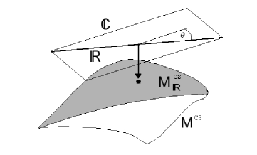
Figure 4.1: The local moduli space $\mathcal{M}_{\mathbb{R}}=\mathcal{M}_{\mathbb{R}}^{\rm cs}\times\mathbb{R}$ in $\mathcal{M}^{\rm cs}\times\mathbb{C}\simeq\mathcal{M}^{\rm cs}\times H^{(3,0)}$.

In fact the proper starting point is not $\mathcal{M}^{\rm cs}_{\mathbb{R}}$ but rather $\mathcal{M}_{\mathbb{R}}=\mathcal{M}_{\mathbb{R}}^{\rm cs}\times\mathbb{R}$ which is the local product of the moduli space of real complex structure deformations of a Calabi-Yau orientifold times the real dilaton direction. The $N=2$ analog of $\mathcal{M}_{\mathbb{R}}$ is the extended moduli space $\hat{\mathcal{M}}^{\rm cs}=\mathcal{M}^{\rm cs}\times\mathbb{C}$ where $\mathbb{C}$ is the complex line normalizing $\Omega$. The corresponding modulus can be identified with the complex dilaton [122]. The orientifold projection fixes the phase of the complex dilaton (it projects out the four-dimensional $B_{2}$) to be $\theta$ and thus reduces $\mathbb{C}$ to $\mathbb{R}$ (figure 4.1). The local geometry of $\mathcal{M}_{\mathbb{R}}$ is encoded in the variations of the real and imaginary part of the normalized holomorphic three-form $C\Omega$. This form naturally defines an embedding

$$E:\mathcal{M}_{\mathbb{R}}\rightarrow V\times V^{*}=\ H^{3}_{+}(\mathbb{R})\times H^{3}_{-}(\mathbb{R})\ .$$ (4.51)

where $V=H^{3}_{+}(\mathbb{R})$ and we used the intersection form $\big{<}\alpha,\beta\big{>}=\int\alpha\wedge\beta$ on $H^{3}(Y)$ to identify $V^{*}\cong H^{3}_{-}(\mathbb{R})$. $V\times V^{*}$ naturally admits a symplectic form $\mathcal{W}$ and an indefinite metric $\mathcal{G}$ defined as

$$\mathcal{W}((\alpha_{+},\alpha_{-}),(\beta_{+},\beta_{-}))=\big{<}\alpha_{+},\beta_{-}\big{>}-\big{<}\beta_{+},\alpha_{-}\big{>}\ ,$$

$$\mathcal{G}((\alpha_{+},\alpha_{-}),(\beta_{+},\beta_{-}))=\big{<}\alpha_{+},\beta_{-}\big{>}+\big{<}\beta_{+},\alpha_{-}\big{>}\ ,$$ (4.52)

where $\alpha_{\pm},\beta_{\pm}\in H^{3}_{\pm}(\mathbb{R})$.

Now we construct $E$ in such a way that $\mathcal{M}_{\mathbb{R}}$ is a Lagrangian submanifold of $V\times V^{*}$ with respect to $\mathcal{W}$ and its metric is induced from $\mathcal{G}$, i.e.

$$E^{*}(\mathcal{W})=0\ ,\qquad E^{*}(\mathcal{G})=g$$ (4.53)

where

$$\tfrac{1}{2}g=dD\otimes dD+G_{KL}dq^{K}\otimes dq^{L}\$$ (4.54)

is the metric on $\mathcal{M}_{\mathbb{R}}$ as determined in (3.75). As we are going to show momentarily $E$ is given by

$$E(q^{\hat{K}})=2\,\big{(}{\mathcal{U}},-e^{2D}{\mathcal{\hat{U}}}\big{)}\ ,$$ (4.55)

where ${\mathcal{U}}+i\,{\mathcal{\hat{U}}}=C\Omega$, $q^{\hat{K}}=(e^{-D},q^{K})$ and $\Omega$ is evaluated at $q^{K}\in\mathcal{M}^{\rm cs}_{\mathbb{R}}$. Additionally $E$ satisfies

$$\mathcal{G}(E(q^{\hat{K}}),E(q^{\hat{K}}))=4\ ,$$ (4.56)

for all $q^{K}$. This implies that the image of all points in $\mathcal{M}_{\mathbb{R}}$ have the same distance from the origin. Later on we will show that this translates into the no-scale condition (4.50).

Let us first show that the $E$ given in (4.55) indeed satisfies (4.53) and (4.56). The explicit calculation is straightforward and essentially included in the calculation presented in section 4.1.2. In order to connect with section 4.1.2 let us first recall how we applied the map (4.4) to extract the chiral data of the $N=1$ moduli space. We started with a special Kähler manifold $\mathcal{M}^{\rm sk}$ with metric determined in terms of a holomorphic prepotential $\mathcal{F}(Z)$. Next we assumed that the $N=2$ theory with quaternionic space $\mathcal{M}^{\rm Q}$ constructed via the local c-map (4.2) allows a reduction to $N=1$. Accordingly the section $\Omega(z)=Z^{\hat{K}}\alpha_{\hat{K}}-\mathcal{F}_{\hat{K}}\beta^{\hat{K}}$ fulfills equation (3.98) for some basis

$$(\alpha_{k},\beta^{\lambda})\in H^{3}_{+}\ ,\qquad(\alpha_{\lambda},\beta^{k})\in H^{3}_{-}\ .$$ (4.57)

Using this basis we found the kinetic potential $\tilde{K}(L,l)$ given in (4.42), which explicitly depends on the prepotential $\mathcal{F}$. It encodes the metric on $\tilde{\mathcal{M}}^{\rm Q}\subset\mathcal{M}^{\rm Q}$ via the Kähler potential (4.16). On the other hand, equation (4.15) defines the complex structure on $\tilde{\mathcal{M}}^{\rm Q}$.

These steps can be translated into the language of this section. Namely, choosing the basis (4.57) to expand the map $E$ defined in (4.55) one finds

$$E(q^{\hat{K}})\ =\ \big{(}2l^{k}\alpha_{k}+\tfrac{1}{4}\tilde{K}_{L^{\lambda}}\beta^{\lambda},2L^{\lambda}\alpha_{\lambda}+\tfrac{1}{4}\tilde{K}_{l^{k}}\beta^{k}\big{)}\ ,$$ (4.58)

where $l^{k},L^{\lambda}$ and $\tilde{K}_{L^{\lambda}},\tilde{K}_{l^{k}}$ are functions of $q^{\hat{K}}$ as given in (4.38) and (4.43). We define coordinates $u^{\hat{K}}=(2l^{k},\tfrac{1}{4}\tilde{K}_{L^{\lambda}})$ on $V$ and coordinates $v_{\hat{K}}=(\tfrac{1}{4}\tilde{K}_{l^{k}},-2L^{\lambda})$ on $V^{*}$. In these coordinates the first two conditions in (4.53) simply read

$$E^{*}(du^{\hat{K}}\wedge dv_{\hat{K}})=0\ ,\qquad E^{*}(du^{\hat{K}}\otimes dv_{\hat{K}})=g\ .$$ (4.59)

From section 4.1.2 we further know that $\tilde{K}_{L^{\kappa}},\tilde{K}_{l^{k}}$ are derivatives of a kinetic potential $\tilde{K}$ and thus we can evaluate $du^{\hat{K}}$ and $dv_{\hat{K}}$ in terms of $l^{k},L^{\kappa}$. Inserting the result into (4.59) the second equation can be rewritten as

$$\tfrac{1}{2}g\ =\ \tfrac{1}{4}\tilde{K}_{l^{k}l^{l}}\,dl^{k}\otimes dl^{l}-\tfrac{1}{4}\tilde{K}_{L^{\kappa}L^{\lambda}}\,dL^{\kappa}\otimes dL^{\lambda}\ ,$$ (4.60)

while the first equation is trivially fulfilled due to the symmetry of $\tilde{K}_{l^{k}l^{l}}$ and $\tilde{K}_{L^{\kappa}L^{\lambda}}$. This metric is exactly the one appearing in the action (4.1.2) when using (4.41). Expressing $g$ in coordinates $e^{D},q^{K}$ leads to (4.54), as we have already checked by going from (4.1.2) to (4.1.2) above. Furthermore, inserting (4.58) into (4.56) it exactly translates into the no-scale condition (4.49), which was shown in section 4.1.2 to be equivalent to (3.96).

We have just shown that $\mathcal{M}_{\mathbb{R}}$ is a Lagrangian submanifold of $V\times V^{*}$. Identifying $T^{*}V\cong V\times V^{*}$ we conclude that $\mathcal{M}_{\mathbb{R}}$ can be obtained as the graph $(\alpha(u),u)$ of a closed one-form $\alpha$. This implies that we can locally find a generating function $K^{\prime}:V\rightarrow\mathbb{R}$ such that $\alpha=dK^{\prime}$. In local coordinates $(v_{\hat{K}},u^{\hat{K}})$ this amounts to

$$v_{\hat{K}}(u)=\frac{\partial K^{\prime}}{\partial u^{{\hat{K}}}}$$ (4.61)

such that

$$-L^{\kappa}(u)=2\,\frac{\partial K^{\prime}(u)}{\partial\tilde{K}_{L^{\kappa}}}\ ,\quad\tilde{K}_{l^{k}}(u)=2\,\frac{\partial K^{\prime}(u)}{\partial l^{k}}\ .$$ (4.62)

These equations are satisfied if we define $K^{\prime}$ in terms of $\tilde{K}$ as

$$2K^{\prime}\ =\ \tilde{K}(L(u),l)-\tilde{K}_{L^{\kappa}}(u)\,L^{\kappa}(u)\ ,$$ (4.63)

which is nothing but the Legendre transform of $\tilde{K}$ with respect to $L^{\kappa}$. Later on we show that the function ${2}K^{\prime}$ is identified with the Kähler potential $K$ given in (3.95).

In order to do that, we now extend our discussion to the full moduli space $\tilde{\mathcal{M}}^{\rm Q}$ including the scalars $\zeta^{\hat{K}}=(\xi^{k},\tilde{\xi}_{\kappa})$ parameterizing the three-form $\hat{C}_{3}$ in $H^{3}_{+}(\mathbb{R})$. Locally one has

$$\tilde{\mathcal{M}}^{\rm Q}=\mathcal{M}_{\mathbb{R}}\times H^{3}_{+}(\mathbb{R})\ .$$ (4.64)

The tangent space at a point $p$ in $\tilde{\mathcal{M}}^{\rm Q}$ can be identified as

$$T_{p}\tilde{\mathcal{M}}^{\rm Q}\cong H^{3}_{+}(\mathbb{R})\oplus H^{3}_{+}(\mathbb{R})\cong H^{3}_{+}(\mathbb{R})\otimes\mathbb{C}\ ,$$ (4.65)

where the first isomorphism is induced by the embedding $E$ given in (4.55). This is a complex vector space and thus $\tilde{\mathcal{M}}^{\rm Q}$ admits an almost complex structure $I$. In components it is given by

$$I(\partial_{q^{\hat{K}}})=(\partial u^{\hat{L}}/\partial q^{\hat{K}})\,\partial_{\zeta^{\hat{L}}}\ ,\qquad I((\partial u^{\hat{L}}/\partial q^{\hat{K}})\,\partial_{\zeta^{\hat{L}}})=-\partial_{q^{\hat{K}}}\ ,$$ (4.66)

where we have used that $I$ is induced by the embedding map $E$. One can show that the almost complex structure $I$ is integrable, since

$$dw^{\hat{K}}=du^{\hat{K}}+id\zeta^{\hat{K}}=(\partial u^{\hat{L}}/\partial q^{\hat{K}})dq^{\hat{K}}+id\zeta^{\hat{K}}\ ,$$ (4.67)

are a basis of $(1,0)$ forms and $w^{\hat{K}}=u^{\hat{K}}+i\zeta^{\hat{K}}$ are complex coordinates on $\tilde{\mathcal{M}}^{\rm Q}$. Using the definition of $u^{\hat{K}}$ one infers that as expected $w^{\hat{K}}=(N^{k},T_{\kappa})$. Moreover, one naturally extends the metric $g$ on $T\mathcal{M}_{\mathbb{R}}$ to a hermitian metric on $T\tilde{\mathcal{M}}^{\rm Q}$. The corresponding two-form is then given by

$$\tilde{\omega}(\partial_{\zeta^{\hat{L}}},\partial_{q^{\hat{K}}})=g(I\partial_{\zeta^{\hat{L}}},\partial_{q^{\hat{K}}})\ ,\qquad\tilde{\omega}(\partial_{\zeta^{\hat{K}}},\partial_{\zeta^{\hat{L}}})=\tilde{\omega}(\partial_{q^{\hat{K}}},\partial_{q^{\hat{L}}})=0\ .$$ (4.68)

Using the definition (4.66) of the almost complex structure and equation (4.53), one concludes that $\tilde{\omega}$ is given by

$$\tilde{\omega}=dv_{\hat{K}}\wedge d\zeta^{\hat{K}}=2i\frac{\partial^{2}K^{\prime}}{\partial w^{\hat{K}}\partial\bar{w}^{\hat{L}}}dw^{\hat{K}}\wedge d\bar{w}^{\hat{L}}\ ,$$ (4.69)

where for the second equality we applied (4.61) and expressed the result in coordinates $w^{\hat{K}}=u^{\hat{K}}+i\zeta^{\hat{K}}$. Note that $K^{\prime}$ is a function of $u^{\hat{K}}$ only, such that derivatives with respect to $w^{\hat{K}}$ translate to ones with respect to $u^{\hat{K}}$. Equation (4.69) implies that $K^{\rm Q}=2K^{\prime}$ is indeed the correct Kähler potential for the moduli space $\tilde{\mathcal{M}}^{\rm Q}$.

So far we restricted ourselves to type IIA orientifolds. However, by using the mirror map (3.5.2) one easily translates the above construction to IIB setups. In the IIB case the real manifold started with is simply the local product $\mathcal{M}^{B}_{\mathbb{R}}=\mathcal{M}^{\rm ks}_{\mathbb{R}}\times\mathbb{R}$, where $\mathcal{M}^{\rm ks}_{\mathbb{R}}$ is a real slice in the complexified Kähler cone $\mathcal{M}^{\rm ks}$ and $\mathbb{R}$ parameterizes the four-dimensional dilaton direction. $\mathcal{M}^{\rm ks}_{\mathbb{R}}$ is locally spanned by the fields $v^{\alpha}$ and $b^{a}$ introduced in section 3.3. Once again we aim to find the embedding map $E$

$$E:\mathcal{M}^{B}_{\mathbb{R}}\rightarrow V\times V^{*}\ .$$ (4.70)

In order to be more explicit we distinguish $O3/O7$ and $O5/O9$ setups and define

$$E_{O3/7}(q^{\hat{K}})\ =\ 2\,({\mathcal{E}},\ e^{2D_{B}}{\mathcal{\hat{E}}})\ ,\qquad E_{O5/9}(q^{\hat{K}})\ =\ 2\,({\mathcal{\hat{E}}},\ e^{2D_{B}}{\mathcal{E}})\ ,$$ (4.71)

where ${\mathcal{E}}+i{\mathcal{\hat{E}}}=e^{-\phi}e^{-B+iJ}$ and $q^{{\hat{A}}}=(e^{-D_{B}},v^{\alpha},b^{a})$. Correspondingly we need to set

$$V_{O3/7}=H^{ev}_{+}\ ,\quad V_{O3/7}^{*}=H^{ev}_{-}\qquad V_{O5/9}=H^{ev}_{-}\ ,\quad V_{O5/9}^{*}=H^{ev}_{+}\ ,$$ (4.72)

where we have abbreviated

$$H^{ev}_{+}=H^{(0,0)}_{+}\oplus H^{(1,1)}_{-}\oplus H^{(2,2)}_{+}\ ,\qquad H^{ev}_{-}=H^{(1,1)}_{+}\oplus H^{(2,2)}_{-}\oplus H^{(3,3)}_{+}\ .$$ (4.73)

Given a vector space $V$ of even forms, the identification of $V^{*}$ with the respective cohomology groups is done by using the intersection form $\big{<}\cdot,\cdot\big{>}$ defined in (3.50). To check that $E_{O3/7}$ and $E_{O5/9}$ are defined correctly, one proceeds in full analogy to the type IIA case. Once again, the calculation simplifies considerably by using the existence of the kinetic potentials (4.23) and (4.31).

Let us summarize our results. We constructed the metric and complex structure of the Kähler manifold $\tilde{\mathcal{M}}^{\rm Q}\subset\mathcal{M}^{\rm Q}$ by specifying a map

$$E:\mathcal{M}_{\mathbb{R}}\rightarrow V\times V^{*}\ ,$$ (4.74)

where $\mathcal{M}_{\mathbb{R}}$ parameterizes the real four-dimensional dilaton direction times certain deformations of the Calabi-Yau orientifold. $V$ is an appropriately chosen vector space

$$V_{IIA}=H^{odd}_{+}\ ,\qquad V_{IIB}=H^{ev}_{\pm}\ ,$$ (4.75)

where $H^{odd}_{+}=H^{3}_{+}$ and $H^{ev}_{\pm}$ is given in (4.73). More explicitly $E$ takes the form

$$E(q^{\hat{K}})=2\,\big{(}\rho,-\hat{\rho}/\Phi_{A,B}\big{)}\ ,$$ (4.76)

where $\Phi_{A,B}(\rho)$ is given in (3.49), (3.58) and $\rho=({\mathcal{U}},{\mathcal{E}},{\mathcal{\hat{E}}})$ depending on the orientifold setup. In order to evaluate $\Phi_{A,B}(\rho)=e^{-2D}$ we use the definition of the four-dimensional dilaton (3.39). Since $\mathcal{M}_{\mathbb{R}}$ is embedded as a Lagrange submanifold in $V\times V^{*}$ it can be locally given by the graph of the one-form $dK^{\prime}$. Moreover, since $E$ induces the metric on $\mathcal{M}_{\mathbb{R}}$ and a complex structure on $\mathcal{M}_{\mathbb{R}}\times V$ the function $2K^{\prime}$ is nothing but the Kähler potential on the local moduli space $\tilde{\mathcal{M}}^{\rm Q}=\mathcal{M}_{\mathbb{R}}\times V$. Thus, the difficulty is to find the map $E$ or, by recalling (4.61), the functional dependence $\hat{\rho}(\rho)$. This non-linear map

$$\rho\ \mapsto\ \hat{\rho}(\rho)\ ,$$ (4.77)

lies at the heart of Hitchins approach to extract the geometry of even and odd forms on six-manifolds [83, 76]. One may thus hope to generalize Calabi-Yau orientifolds to non-Calabi-Yau orientifolds [118].

Chapter 5 Calabi-Yau orientifolds with NS-NS and R-R background fluxes

In this chapter we redo the reduction of type IIB and type IIA on Calabi-Yau orientifolds by additionally allowing for non-trivial R-R and NS-NS background fluxes. As we will show, these fluxes result in non-trivial potentials for the supergravity fields and can lead to charged scalars or massive tensors.

We first discuss the two type IIB setups. In section 5.1 we show that in orientifolds with $O3/O7$ planes fluxes introduce a superpotential only. More intriguingly, we point out in section 5.2 that $O5/O9$ setups with background flux in general admit a superpotential as well as a massive linear multiplet. Thus, additionally to the kinetic terms studied in section 4.1.1 we find $D-$terms and a direct mass term for a linear multiplet [39, 78]. In both IIB orientifold cases the induced potentials depend only on some but not all bulk moduli fields in the theory. In order to find potentials for the remaining moduli one has to take non-perturbative contributions into account. In [42] it was argued that certain D-instantons induce corrections to the superpotential. To gain a better understanding of these corrections is subject of various recent work [44, 47]. In section 5.4 we do only a very moderate step and check if the resulting leading order superpotentials are holomorphic in the bulk coordinates. Assuming a generic form of such a superpotential one might achieve that all bulk fields are stabilized in the vacuum [35, 44, 47].

In type IIA orientifolds the situation is slightly different. As we show in section 5.3 generic NS-NS and R-R background fluxes induce a superpotential which depends on all bulk moduli of the theory. Hence, appropriately chosen background fluxes could stabilize all geometric moduli in type IIA orientifolds. Additionally, one can attempt to include corrections due to non-perturbative effects. A brief discussion of superpotential contributions due to world-sheet or D-instantons can be found in section 5.4.

5.1 $O3/O7$ orientifolds: GVW superpotential

In this section we study $O3/O7$ orientifolds by also allowing background three-form fluxes $H_{3}$ and $F_{3}$ on the Calabi-Yau manifold [13, 17, 18, 20, 39]. The Bianchi identities together with the equations of motion imply that $H_{3}$ and $F_{3}$ have to be harmonic three-forms. In orientifold compactifications they are further constrained by the orientifold projection. From (3.20) we see that for the projection given in (3.10) they both have to be odd under $\sigma^{*}$ and hence are parameterized by elements of $H^{(3)}_{-}(Y)$. It is convenient to combine the two three-forms into a complex $G_{3}$ according to

$$G_{3}=F_{3}-\tau H_{3}\ ,\qquad\tau=C_{0}+ie^{-\phi}\ .$$ (5.1)

$G_{3}$ can be explicitly expanded into a symplectic basis of $H^{(3)}_{-}$ as

$$G_{3}=m^{\hat{k}}\alpha_{\hat{k}}-e_{\hat{k}}\beta^{\hat{k}}\ ,\qquad\hat{k}=0,\ldots,h^{(1,2)}\ ,$$ (5.2)

with $2(h^{(1,2)}_{-}+1)$ complex flux parameters

$$m^{\hat{k}}=m^{\hat{k}}_{F}-\tau m^{\hat{k}}_{H}\ ,\qquad e_{\hat{k}}=e_{\hat{k}}^{F}-\tau e_{\hat{k}}^{H}\ .$$ (5.3)

However, in the following we do not need this explicit expansion and express our results in terms of $G_{3}$.

The reduction of the IIB theory is performed by replacing

$$d\hat{B}_{2}\ \rightarrow\ d\hat{B}_{2}+H_{3}\ ,\qquad d\hat{C}_{2}\ \rightarrow\ d\hat{C}_{2}+F_{3}\ ,$$ (5.4)

in the field-strengths (2.28). $H_{3}$ and $F_{3}$ are the background value of the field strengths $\hat{F}_{3}$ and $\hat{H}_{3}$ but do not effect $\hat{F}_{5}$ since the only possible terms would be of the form $H_{3}\wedge C_{2}$ or $B_{2}\wedge F_{3}$ but both $C_{2}$ and $B_{2}$ are projected out by the orientifold projection. The only effect of non-trivial background fluxes is the appearance of a potential $V$. It is manifestly positive semi-definite and found to be [17, 20, 27, 29]

$$V=e^{K}\Big{(}\int\Omega\wedge\bar{G}_{3}\int\bar{\Omega}\wedge G_{3}+G^{k{l}}\int\chi_{k}\wedge G_{3}\int\bar{\chi}_{l}\wedge\bar{G}_{3}\Big{)}\ ,$$ (5.5)

where $K$ is given in (3.46), $\chi_{k}$ is a basis of $H^{(2,1)}_{-}$ defined in (3.23) and the background flux $G_{3}$ is defined in (5.1). The details of the computation of $V$ can be found in [20, 39].

Strictly speaking the additional term $\mathcal{L}^{(4)}_{\text{top}}\sim\int_{Y}H_{3}\wedge F_{3}$ arises in the Kaluza-Klein reduction. However, consistency of the compactifications requires its cancellation against Wess-Zumino like couplings of the orientifold planes to the R-R flux [20].

Finally, one checks that the potential (5.5) can be derived from a superpotential $W$ via the expression given in (3.41) with vanishing $D$-term $D_{\kappa}=0$. For orientifolds with $c^{a}=b^{a}=0$ $W$ was shown to be [15, 17, 20, 27, 29]

$$W(\tau,z^{k})=\int_{Y}\Omega\wedge G_{3}\ .$$ (5.6)

This continues to be the correct superpotential also if $c^{a}$ and $b^{a}$ are in the spectrum [39], which is due to the fact that $K^{\rm Q}$ satisfies the no-scale condition (3.51). This ends our analysis for $O3/O7$ setups. Surprisingly, for $O5/O9$ orientifolds the computation is more involved and forces us to once more apply and extend the linear multiplet techniques developed in chapter 4.

5.2 $O5/O9$ orientifolds: Gaugings and the massive linear multiplet

We now turn to the effective action of $O5/O9$ orientifolds with background fluxes. In order to detect the changes due to this non-trivial background, we proceed as in the $O3/O7$ case and first evaluate the field strengths (2.28) including the possibility of background three-form fluxes $H_{3}$ and $F_{3}$. Since $\hat{B}_{2}$ and hence $H_{3}$ is odd it is again parameterized by $H^{(3)}_{-}$ while $\hat{C}_{2}$ and $F_{3}$ are even and therefore parameterized by $H^{(3)}_{+}$. As a consequence the explicit expansions of the background fluxes $H_{3}$ and $F_{3}$ are given by

$$H_{3} = m^{k}_{H}\alpha_{k}-e_{k}^{H}\beta^{k}\ ,\qquad k=1,\ldots,h^{(2,1)}_{-}\ ,$$

$$F_{3} = m_{F}^{\hat{\kappa}}\,\alpha_{\hat{\kappa}}-e^{F}_{\hat{\kappa}}\,\beta^{\hat{\kappa}}\ ,\qquad\hat{\kappa}=0,\ldots,h^{(2,1)}_{+}\ ,$$ (5.7)

where the $(m^{k}_{H},e_{k}^{H})$ are $2h^{(2,1)}_{-}$ constant flux parameters determining $H_{3}$ and $(m_{F}^{\hat{\kappa}},e^{F}_{\hat{\kappa}})$ are $2h^{(2,1)}_{+}+2$ constant flux parameters corresponding to $F_{3}$. Inserting (3.24), (3.26) and (5.2) into (2.28) we obtain

$$\hat{H}_{3} = db^{a}\wedge\omega_{a}+m^{k}_{H}\alpha_{k}-e_{k}^{H}\beta^{k}\ ,\qquad\hat{F}_{3}\ =\ dC_{2}+dc^{\alpha}\wedge\omega_{\alpha}+F_{3}\ ,$$

$$\hat{F}_{5} = dD_{2}^{a}\wedge\omega_{a}+\tilde{F}^{k}\wedge\alpha_{k}-\tilde{G}_{k}\wedge\beta^{k}+d\rho_{a}\wedge\tilde{\omega}^{a}$$

$$-db^{a}\wedge C_{2}\wedge\omega_{a}-c^{\alpha}db^{a}\omega_{a}\wedge\omega_{\alpha}\ ,$$

where we defined

$$\tilde{F}^{k}=dV^{k}-m^{k}_{H}C_{2}\ ,\qquad\tilde{G}_{k}=dU_{k}-e_{k}^{H}C_{2}\ .$$ (5.9)

As in section 3.3 the self-duality condition on $\hat{F}_{5}$ is imposed by a Lagrange multiplier [24] and we eliminate $D^{a}_{2}$ and $U_{k}$ by inserting their equations of motion into the action. After Weyl rescaling the four-dimensional metric with a factor $\mathcal{K}/6$ the ${N}=1$ effective action reads

$$S^{(4)}_{O5/O9} = \int-\tfrac{1}{2}R*\mathbf{1}-G_{\kappa\lambda}\;dz^{\kappa}\wedge*d\bar{z}^{\lambda}-G_{\alpha\beta}\;dv^{\alpha}\wedge*dv^{\beta}-G_{ab}\;db^{a}\wedge*db^{b}$$

$$-\tfrac{e^{2D}}{6}\mathcal{K}\,G_{\alpha\beta}\;dc^{\alpha}\wedge*dc^{\beta}-\tfrac{e^{-2D}}{24}\mathcal{K}\,dC_{2}\wedge*dC_{2}-\tfrac{1}{4}dC_{2}\wedge(\rho_{a}db^{a}-b^{a}d\rho_{a})$$

$$-dD\wedge*dD-\tfrac{3e^{2D}}{8\mathcal{K}}G^{ab}(d\rho_{a}-\mathcal{K}_{ac\alpha}c^{\alpha}db^{c})\wedge*(d\rho_{b}-\mathcal{K}_{bd\beta}c^{\beta}db^{d})-V*\mathbf{1}$$

$$+\tfrac{1}{4}\text{Re}\;\mathcal{M}_{kl}\;\tilde{F}^{k}\wedge\tilde{F}^{l}+\tfrac{1}{4}\text{Im}\;\mathcal{M}_{kl}\;\tilde{F}^{k}\wedge*\tilde{F}^{l}+\tfrac{1}{4}e_{k}(dV^{k}+\tilde{F}^{k})\wedge C_{2}\ ,$$

where

$$V =\frac{18i\ e^{4\phi}}{\mathcal{K}^{2}\int\Omega\wedge\bar{\Omega}}\left(\int\Omega\wedge F_{3}\int\bar{\Omega}\wedge F_{3}+G^{\kappa\lambda}\int\chi_{\kappa}\wedge F_{3}\int\bar{\chi}_{\lambda}\wedge F_{3}\right)$$ (5.11)

$$-\tfrac{9\,e^{2\phi}}{\mathcal{K}^{2}}\Big{[}m^{k}_{H}\,(\text{Im}\mathcal{M})_{kl}\,m^{l}_{H}+\big{(}e_{k}^{H}-(m_{H}\text{Re}\mathcal{M})_{k}\big{)}\big{(}\text{Im}\mathcal{M}\big{)}^{-1kl}\big{(}e_{l}^{H}-(m_{H}\text{Re}\mathcal{M})_{l}\big{)}\Big{]}\ .$$

The derivation of this potential can be found in ref. [39].

The action (5.2) has the standard one-form gauge invariance $V^{k}\to V^{k}+d\Lambda^{k}_{0}$ but due to the modification in (5.9) also a modified (Stückelberg) two-form gauge invariance given by

$$C_{2}\to C_{2}+d\Lambda_{1}\ ,\qquad V^{k}\to V^{k}+m^{k}_{H}\Lambda_{1}\ .$$ (5.12)

Thus for $m^{k}_{H}\neq 0$ one vector can be set to zero by an appropriate gauge transformation. This is directly related to the fact that (5.2) includes mass terms proportional to $m^{k}_{H}$ for $C_{2}$ arising from (5.9). In this case gauge invariance requires the presence of Goldstone degrees of freedom which can be ‘eaten’ by $C_{2}$. Finally note that the last term in (5.2) also includes a standard $D=4$ Green-Schwarz term $F^{k}\wedge C_{2}$.

5.2.1 Vanishing magnetic fluxes $m^{k}_{H}=0$

The next step is to show that $S^{(4)}_{O5/O9}$ is consistent with the constraints of $N=1$ supergravity. However, due to the possibility of $C_{2}$ mass terms this is not completely straightforward. A massive $C_{2}$ is no longer dual to a scalar but rather to a vector. We find it more convenient to keep the massive tensor in the spectrum and discuss the $N=1$ constraints in terms of a massive linear multiplet. Before doing so, let us first discuss the situation $m^{k}_{H}=0$ where $\tilde{F}^{l}=F^{l}$ holds. In this case the $C_{2}$ remains massless and can be dualized to a scalar field $h$ which together with the dilaton $\phi$ combines to form a chiral multiplet $(\phi,h)$. Using the standard dualization procedure (see section 2.3) one obtains the effective action (3.38) plus the potential $V$ given in (5.11) evaluated at $m^{k}_{H}=0$. Furthermore, due to electric NS-NS fluxes the scalar $h$ is gauged and we have to replace in (3.38)

$$dh\quad\rightarrow\quad Dh=dh-e_{k}^{H}V^{k}\ .$$ (5.13)

Hence, $h$ couples non-trivially to the gauge fields as a direct consequence of the Green-Schwarz coupling $F^{k}\wedge C_{2}$ in (5.2). In the dualized action the scalar $h$ then is charged under the $U(1)$ gauge transformation $h\to h+e_{k}^{H}\Lambda_{0}^{k}$ with $V^{k}\to V^{k}+d\Lambda_{0}^{k}$. Note that the gauge charges are set by the electric fluxes.

The Kähler potential (3.56) with chiral coordinates (3.54) and the gauge-couplings (3.61) remain unchanged for the theory with $m^{k}_{H}=0$. However, due to the non-trivial electric NS-NS fluxes the covariant derivative of $h$ given in (5.13) translates into the covariant derivative $DS=dS-ie_{k}V^{k}$. It remains to cast the potential $V$ given in (5.11), evaluated at $m^{k}_{H}=0$, into the standard $N=1$ supergravity form (3.41). From eq. (5.13) we see that the axion is charged and as a consequence we expect a non-vanishing $D$-term in the potential. Recall the general formula for the $D$-term [116]

$$K_{I\bar{J}}\bar{X}^{\bar{J}}_{k}=i\partial_{I}D_{k}\ ,$$ (5.14)

where $X^{I}$ is the Killing vector of the $U(1)$ gauge transformations defined as $\delta M^{I}=\Lambda^{k}_{0}X_{k}^{J}\partial_{J}M^{I}$. Inserting (3.56) and (3.54) we obtain

$$D_{k}=-e_{k}^{H}\,\frac{\partial K}{\partial\bar{S}}=3\,e_{k}^{H}\,e^{\phi}\mathcal{K}^{-1}\ .$$ (5.15)

Using also (3.59) we arrive at the $D$-term contribution to the potential

$$\tfrac{1}{2}(\text{Re}\;f)^{-1\ kl}D_{k}D_{l}=-\tfrac{9}{\mathcal{K}^{2}}e^{2\phi}\;e_{k}^{H}\,(\text{Im}\;\mathcal{M})^{-1\ kl}\,e_{l}^{H}\ ,$$ (5.16)

which indeed reproduces the last term in (5.11) for $m^{k}_{H}=0$.

The first term in (5.11) arises from the superpotential

$$W=\int_{Y}\Omega\wedge F_{3}\ ,$$ (5.17)

which follows from a calculation analog to the $O3/O7$ case [39]. It is interesting that for this class of orientifolds the RR-flux $F_{3}$ results in a contribution to the superpotential while the NS-flux $H_{3}$ contributes instead to a $D$-term.

5.2.2 Non-vanishing magnetic fluxes $m^{k}_{H}\neq 0$

Let us now turn to the case where both electric and magnetic fluxes are non-zero and the two-form $C_{2}$ is massive. In this case $C_{2}$ is dual to a massive vector or equivalently the massive linear multiplet is dual to massive vector multiplet. Here we do not discuss this duality but instead show how the couplings of a massive linear multiplet is consistent with the action (5.2) [78].

In section 4.1.1 we already examined the kinetic terms and couplings for the $O5/O9$ theory in the presence of one tensor multiplet $L=(\phi,C_{2})$. We found that they are determined in terms of the generalized Kähler potential and the function $F$ both given in (4.25). Let us now briefly discuss the situation of a massive linear multiplet coupled to $N=1$ vector- and chiral multiplets. For simplicity we discuss the situation in flat space and do not couple the massive linear multiplet to supergravity. However, we expect our results to generalize to the supergravity case. More details can be found in [117, 78].

As we already said, a linear multiplet $L$ contains a real scalar (also denote by $L$) and the field strength of a two-form $C_{2}$ as bosonic components. However, it does not contain the two-form itself which instead is a member of the chiral ‘prepotential’ $\Phi$ defined as

$$L=D\Phi+\bar{D}\bar{\Phi}\ ,\qquad\bar{D}\Phi=0\ .$$ (5.18)

This definition solves the constraint (4.6) (in flat space). The kinetic term for $L$ (or rather for $\Phi$) is given in (4.7) and a mass-term can be added via the chiral integral

$$\mathcal{L}_{m}=\tfrac{1}{4}\int d^{2}\theta\Big{[}f_{kl}(N)(W^{k}-2im^{k}_{H}\Phi)(W^{l}-2im^{l}_{H}\Phi)+2e_{k}^{H}(W^{k}-im^{k}_{H}\Phi)\Phi\Big{]}+{\rm h.c.}\ ,$$ (5.19)

where $W^{k}=-\tfrac{1}{4}\bar{D}^{2}DV^{k}$ are the chiral field strengths supermultiplets of the vector multiplets $V^{k}$ and $f_{kl}(N)$ are the gauge kinetic function which can depend holomorphically on the chiral multiplets $N$. $(m^{k}_{H},e_{k}^{H})$ are constant parameters which will turn out to correspond to the flux parameters defined in (5.2). The Lagrangian (5.19) is invariant under the standard one-form gauge invariance $V^{k}\to V^{k}+\Lambda_{0}^{k}+\bar{\Lambda}_{0}^{k}$ ($\Lambda_{0}^{k}$ are chiral superfields) which leaves both $W^{k}$ and $\Phi$ invariant. In addition (5.19) has a two-form gauge invariance corresponding to (5.12) given by

$$\Phi\to\Phi+\tfrac{i}{8}\bar{D}^{2}D\Lambda_{1}\ ,\qquad V^{k}\to V^{k}+m^{k}_{H}\Lambda_{1}\ ,$$ (5.20)

where $\Lambda_{1}$ now is a real superfield. From (5.20) we see that one entire vector multiplet can be gauged away and thus plays the role of the Goldstone degrees of freedom which are ‘eaten’ by the massive linear multiplet.

In components one finds the bosonic action

$$\mathcal{L}_{m}=-\tfrac{1}{2}\text{Re}f_{kl}\;\tilde{F}^{k}\wedge*\tilde{F}^{l}-\tfrac{1}{2}\text{Im}f_{kl}\;\tilde{F}^{k}\wedge\tilde{F}^{l}+\tfrac{1}{4}e_{k}(dV^{k}+\tilde{F}^{k})\wedge C_{2}-V*\mathbf{1}\ ,$$ (5.21)

where $\tilde{F}^{l}$ is defined exactly as in (5.9) and the potential $V$ receives two distinct contributions

$$V=\tfrac{1}{2}\,(\text{Re}f)^{-1kl}D_{k}D_{l}+2\,m^{k}_{H}\text{Re}f_{kl}\,m^{l}_{H}\,L^{2}\ ,\qquad D_{k}=\big{(}e_{k}^{H}+2\,\text{Im}f_{kl}\,m^{l}_{H}\big{)}\,L\ .$$ (5.22)

The first term arises from eliminating the $D$-terms in the $U(1)$ field strength $W^{k}$ while the second term is a ‘direct’ mass term for the scalar $L$. Inserting the $D$-term yields a second contribution to the mass term and one obtains altogether

$$V = \tfrac{1}{2}\big{[}\big{(}e_{k}^{H}+2\text{Im}f_{kp}\,m^{p}\big{)}(\text{Re}f)^{-1kl}\big{(}e_{l}^{H}+2\text{Im}f_{lr}\,m^{r}\big{)}+4m^{k}_{H}\,\text{Re}f_{kl}\,m^{l}_{H}\big{]}L^{2}\ .\qquad$$ (5.23)

Using (4.26) and (3.59) this precisely agrees with the second term in the potential (5.11).

As before the first term in (5.11) can be derived from the superpotential (5.17). This ends our discussion of type IIB orientifolds in a general NS-NS and R-R flux background. As we have seen, switching on fluxes yields a potential for only part of the moduli fields. This changes in IIA orientifolds to which we will turn now.

5.3 $O6$ orientifolds: Flux superpotentials

In this section we derive the effective action of type IIA orientifolds in the presence of background fluxes. For standard $N=2$ Calabi-Yau compactifications of type IIA a similar analysis is carried out in refs. [26, 40]. In order to do so we need to start from the ten-dimensional action of massive type IIA supergravity which differs from the action (2.18) in that the two-form $\hat{B}_{2}$ is massive. In the Einstein frame it is given by [125]

$$S^{(10)}_{MIIA} = \int-\tfrac{1}{2}\hat{R}*\mathbf{1}-\tfrac{1}{4}d\hat{\phi}\wedge*d\hat{\phi}-\tfrac{1}{4}e^{-\hat{\phi}}\hat{H}_{3}\wedge*\hat{H}_{3}-\tfrac{1}{2}e^{\frac{3}{2}\hat{\phi}}\hat{F}_{2}\wedge*\hat{F}_{2}$$ (5.24)

$$-\tfrac{1}{2}e^{\frac{1}{2}\hat{\phi}}\hat{F}_{4}\wedge*\hat{F}_{4}-\tfrac{1}{2}e^{\frac{5}{2}\hat{\phi}}\,(m^{0})^{2}*\mathbf{1}+\mathcal{L}_{\rm top}\ ,$$

where

$$\mathcal{L}_{\rm top} = -\tfrac{1}{2}\Big{[}\hat{B}_{2}\wedge d\hat{C}_{3}\wedge d\hat{C}_{3}\ -(\hat{B}_{2})^{2}\wedge d\hat{C}_{3}\wedge d\hat{C}_{1}+\tfrac{1}{3}(\hat{B}_{2})^{3}\wedge(d\hat{C}_{1})^{2}$$ (5.25)

$$-\tfrac{m^{0}}{3}(\hat{B}_{2})^{3}\wedge d\hat{C}_{3}+\tfrac{m^{0}}{4}(\hat{B}_{2})^{4}\wedge d\hat{C}_{1}+\tfrac{(m^{0})^{2}}{20}(\hat{B}_{2})^{5}\Big{]}\ ,$$

and the field strengths are defined as

$$\hat{H}_{3}=d\hat{B}_{2}\ ,\quad\hat{F}_{2}=d\hat{C}_{1}+m^{0}\hat{B}_{2}\ ,\quad\hat{F}_{4}=d\hat{C}_{3}-\hat{C}_{1}\wedge\hat{H}_{3}-\tfrac{m^{0}}{2}(\hat{B}_{2})^{2}\ .$$ (5.26)

Compared to the analysis of the previous section we now include non-trivial background fluxes of the field strengths $F_{2}$, $H_{3}$ and $F_{4}$ on the Calabi-Yau orientifold. We keep the Bianchi identity and the equation of motion intact and therefore expand $F_{2}$, $H_{3}$ and $F_{4}$ in terms of harmonic forms compatible with the orientifold projection. From (3.62) we infer that $F_{2}$ is expanded in harmonic forms of $H^{2}_{-}(Y)$, $H_{3}$ in harmonic forms of $H^{3}_{-}(Y)$ and $F_{4}$ in harmonic forms of $H^{4}_{+}(Y)$. Explicitly the expansions read

$$H_{3}\,=\,q^{\lambda}\alpha_{\lambda}-p_{k}\,\beta^{k}\ ,\quad F_{2}\,=\,-m^{a}\omega_{a}\ ,\quad F_{4}\,=\,e_{a}\,\tilde{\omega}^{a}\ ,$$ (5.27)

where $(q^{\lambda},p_{k})$ are $h^{(2,1)}+1$ real NS flux parameters while $(e_{a},m^{a})$ are $2h^{1,1}_{-}$ real RR flux parameters. The harmonic forms $(\alpha_{\lambda},\beta^{k})$ are the elements of the real symplectic basis of $H^{3}_{-}$ introduced in (3.97). The basis $\tilde{\omega}^{a}$ of $H^{(2,2)}_{+}$ is defined to be the dual basis of $\omega_{a}$ while the basis $\tilde{\omega}^{\alpha}$ denotes a basis of $H^{(2,2)}_{-}$ dual to $\omega_{\alpha}$.

Inserting (3.66), (3.72) and (5.27) into (5.26) we arrive at

$$\hat{H}_{3} = db^{a}\wedge\omega_{a}+q^{\lambda}\alpha_{\lambda}-p_{k}\,\beta^{k}\ ,\qquad\qquad\hat{F}_{2}=(m^{0}b^{a}+m^{a})\,\omega_{a}\ ,$$ (5.28)

$$\hat{F}_{4} = dC_{3}+dA^{\alpha}\wedge\omega_{\alpha}+d\xi^{k}\wedge\alpha_{k}-d\tilde{\xi}_{\lambda}\wedge\beta^{\lambda}+\big{(}b^{a}m^{b}-\tfrac{1}{2}m^{0}b^{a}b^{b}\big{)}\,\mathcal{K}_{abc}\tilde{\omega}^{c}+e_{a}\,\tilde{\omega}^{a}\ ,$$

where we have used $\omega_{a}\wedge\omega_{b}=\mathcal{K}_{abc}\,\tilde{\omega}^{c}$. Now we repeat the KK-reduction of the previous section using the modified field strength (5.28) and the action (5.24) instead of (2.18). This results in

$$S^{(4)}=S^{(4)}_{O6}-\int\tfrac{g}{2}\,dc_{3}\wedge*dc_{3}+{h}\,dc_{3}+U*\mathbf{1}\ ,$$ (5.29)

where $S^{(4)}_{O6}$ is given in (3.75). $c_{3}$ is the four-dimensional part of the ten-dimensional three-form $\hat{C}_{3}$ defined in (3.72) and its couplings to the scalar fields are given by

$$g=e^{-4\phi}\left(\tfrac{\mathcal{K}}{6}\right)^{3}\ ,\qquad h=e_{a}b^{a}+\tilde{\xi}_{\lambda}q^{\lambda}-\xi^{k}p_{k}+\tfrac{1}{2}\text{Re}\mathcal{N}_{0{\hat{a}}}\,m^{\hat{a}}\ ,$$ (5.30)

where we denoted $m^{\hat{a}}=(m^{0},m^{a})$. The potential term $U$ of (5.29) is given by

$$U=\tfrac{9}{\mathcal{K}^{2}}e^{2\phi}\int_{Y}H_{3}\wedge*H_{3}-\tfrac{18}{\mathcal{K}^{2}}e^{4\phi}\text{Im}\mathcal{N}_{{\hat{a}}{\hat{b}}}\,m^{\hat{a}}m^{\hat{b}}+\tfrac{27}{\mathcal{K}^{3}}e^{4\phi}G^{ab}(e_{a}-\text{Re}\mathcal{N}_{a{\hat{a}}}\,m^{\hat{a}})(e_{b}-\text{Re}\mathcal{N}_{b{\hat{b}}}\,m^{\hat{b}})\ .$$ (5.31)

The matrix $\mathcal{N}_{{\hat{a}}{\hat{b}}}(t,\bar{t})$ is defined to be the corresponding part of the $N=2$ gauge-coupling matrix (B.21) restricted to $\tilde{\mathcal{M}}^{\rm SK}$ by applying (3.76) and (3.34).

In four space-time dimensions $c_{3}$ is dual to a constant which plays the role of an additional electric flux $e_{0}$ in complete analogy with the situation in $N=2$ discussed in [26]. Eliminating $c_{3}$ in favor of $e_{0}$ by following [26] or [85] the potential takes the form [41]

$$V=\tfrac{9}{\mathcal{K}^{2}}e^{2\phi}\int H_{3}\wedge*H_{3}-\tfrac{18}{\mathcal{K}^{2}}e^{4\phi}(\tilde{e}_{\hat{a}}-\mathcal{N}_{{\hat{a}}{\hat{c}}}\,m^{\hat{c}})(\text{Im}\mathcal{N})^{-1\,{\hat{a}}{\hat{b}}}(\tilde{e}_{\hat{b}}-\bar{\mathcal{N}}_{{\hat{b}}{\hat{c}}}\,m^{\hat{c}})\ ,$$ (5.32)

where we introduced the shorthand notation $\tilde{e}_{\hat{a}}=(e_{0}+\xi_{\lambda}q^{\lambda}-\xi^{\hat{k}}p_{\hat{k}},e_{a})$ and $m^{\hat{a}}=(m^{0},m^{a})$. Note that in the presence of NS flux one can absorb $e_{0}$ by shifting the fields $\xi,\tilde{\xi}$. This corresponds to adding an integral form to $C_{3}$ as carefully discussed in [85]. However, for the discussion of mirror symmetry it is more convenient to keep the parameter $e_{0}$ explicitly in the action.

In order to establish the consistency with $N=1$ supergravity one needs to rewrite $V$ given in (5.32) in terms of (3.41) or in other words we need express $V$ in terms of a superpotential $W$ and appropriate $D$-terms. From (5.29) we infer that turning on fluxes does not charge any of the fields and therefore all $D$-terms have to vanish. In [41] it was checked that the potential (5.32) can be entirely expressed in terms of the superpotential

$$W\ =\ W^{\rm Q}(N,T)+W^{\rm K}(t)\ ,$$ (5.33)

where

$$W^{\rm Q}(N^{k},T_{\lambda}) = \int_{Y}\Omega_{\rm c}\wedge H_{3}\ =\ -2N^{k}p_{k}-iT_{\lambda}q^{\lambda}\ ,$$ (5.34)

$$W^{\rm K}(t^{a}) = e_{0}+\int_{Y}J_{\rm c}\wedge F_{4}-\tfrac{1}{2}\int_{Y}J_{\rm c}\wedge J_{\rm c}\wedge F_{2}-\tfrac{1}{6}m^{0}\int_{Y}J_{\rm c}\wedge J_{\rm c}\wedge J_{\rm c}\ ,$$

$$= e_{0}+e_{a}t^{a}+\tfrac{1}{2}\mathcal{K}_{abc}m^{a}t^{b}t^{c}-\tfrac{1}{6}m^{0}\mathcal{K}_{abc}t^{a}t^{b}t^{c}\ ,$$

and $\Omega_{\rm c}$ and $J_{\rm c}$ are defined in (3.102). Using the definitions (3.50) and (3.104) of the skew-symmetric products $\big{<}\cdot,\cdot\big{>}$ for even and odd forms $W$ is rewritten as

$$W=\big{<}e^{J_{\rm c}},F\big{>}+\big{<}\Omega_{\rm c},H_{3}\big{>}\ ,\qquad F=m^{0}-F_{2}-F_{4}+F_{6}\ ,$$ (5.35)

where we have defined $F_{6}$ via $e_{0}=\int_{Y}F_{6}$. We see that the superpotential is the sum of two terms. $W^{\rm Q}$ depends on the NS fluxes $(p_{k},q^{\lambda})$ of $H_{3}$ and the chiral fields $N^{k},T_{\lambda}$ parameterizing the space $\tilde{\mathcal{M}}^{\rm Q}$. $W^{\rm K}$ depends on the RR fluxes $(e_{\hat{a}},m^{\hat{b}})$ of $F_{2}$ and $F_{4}$ (together with $m^{0}$ and $e_{0}$) and the complexified Kähler deformations $t^{a}$ parameterizing $\mathcal{M}^{\rm SK}$. We see that contrary to the type IIB case both types of moduli, Kähler and complex structure deformations appear in the superpotential suggesting the possibility that all moduli can be fixed in this set-up. This was resently shown to be the case in refs. [80, 79].

Let us end this section by comparing the R-R superpotentials of type IIA and type IIB orientifolds. Recall that for both IIB orientifold setups R-R fluxes induce superpotentials (5.6) and (5.17) holomorphic in the complex structure deformations $z$. Hence, we compare

$$W_{A}(t)=\big{<}e^{J_{\rm c}},F\big{>}\ ,\qquad W_{B}(z)=\big{<}\Omega,F_{3}\big{>}\ ,$$ (5.36)

where the skew-products are defined in (3.50) and (3.104). As just discussed $F$ depends on $2h^{(1,1)}_{-}+2$ RR fluxes $(e_{\hat{a}},m^{\hat{a}})$. To count the flux parameters labeling $F_{3}$ recall that it transforms differently in the two IIB orientifolds. $F_{3}$ sits in $H^{3}_{-}(\tilde{Y})$ and is determined in terms of $2h^{(2,1)}_{-}+2$ real flux parameters for the $O3/O7$ case and sits in $H^{3}_{+}(\tilde{Y})$ depending on $2h^{(2,1)}_{+}+2$ real flux parameters for the $O5/O9$ case. Therefore, the number of flux parameters matches when choosing mirror involutions satisfying (3.5). Exchanging [126]

$$e^{J_{\rm c}}(t)\ \leftrightarrow\ \Omega(z)\ ,\qquad F\ \leftrightarrow\ F_{3}\ ,$$ (5.37)

as in equation (3.108) the two superpotentials $W_{A}(t)$ and $W_{B}(z)$ get identified. In $N=2$ the mirror identification of the complex structure moduli space $\mathcal{M}^{\rm cs}$ with the complexified Kähler moduli space $\mathcal{M}^{\rm ks}$ can be used to calculate world-sheet instanton corrections to $\mathcal{M}^{\rm ks}$. It would be interesting to generalize this to $N=1$ orientifold theories which allow additionally for non-oriented world-sheets as discussed at the end of section 3.4. In addition to world-sheet instantons also certain D-instantons induce correction terms to the superpotential. We will end this chapter by a few comments on their generic structure.

5.4 D-instanton corrections to the superpotentials

Let us close this chapter by briefly discussing possible D-instanton corrections to the superpotentials (5.6), (5.17) and (5.33). They can arise from wrapping $D(p-1)$-branes around $p$-cycles $\Sigma_{p}$ [104]. In addition to corrections of the Kähler potential D-instantons induce extra superpotential terms [42]. These depend on brane moduli as well as bulk fields and found recent phenomenological application in moduli stabilization [35, 44, 47]. It would be interesting to fully incorporate these effects and to understand the additional contributions due to non-orientable world-volumes. First steps into this direction are done in the recent works [44, 47]. In this section we will take only a very moderate step and apply the calibration conditions to show that the D-brane action becomes linear in the bulk fields. This ensures holomorphicity of the induces superpotential terms when expressed in the proper Kähler variables of the respective orientifold setup.

To make this more precise, recall that any correlation function is weighted by the string-frame world-volume action of the wrapped Euclidean $D(p-1)$-branes and thus includes a factor $e^{-S_{D(p-1)}}$ where

$$S_{D(p-1)}=i\mu_{p}\,\int_{\mathcal{W}_{p}}\Big{(}d^{p}\lambda\ e^{-\hat{\phi}}\sqrt{\det\big{(}{\varphi^{*}(\hat{g}+\hat{B}_{2})+\ell F}\big{)}}-i\varphi^{*}\Big{(}\sum_{q}\hat{C}_{q}\wedge e^{-\hat{B}_{2}}\Big{)}\wedge e^{\ell F}\Big{)}\ .$$ (5.38)

where $\ell=2\pi\alpha^{\prime}$. This is the Euclidean analog of the Dirac-Born-Infeld action (3.1) plus the Chern-Simons action (3.2). $\mathcal{W}_{p}$ is the world-volume of the $D(p-1)$-brane and $\varphi^{*}$ is the pull-back of the map $\varphi$ which embeds $\mathcal{W}_{p}$ into Calabi-Yau orientifold $Y$, $\varphi:\mathcal{W}_{p}\hookrightarrow Y$. We have chosen the R-R charge $\mu_{p}$ equal to the tension since the wrapped $D(p-1)$-branes must be BPS in order to preserve $N=1$ supersymmetry. In fact, as we already discussed in section (3.1) there are additional condition arising from the requirement that the $Dp$-branes preserves the same supersymmetry that is left intact by the orientifold projections. This in turn implies that $O3/O7$ orientifolds can admit corrections from $D3$ instantons, $O5/O9$ setups from $D1$ and $D5$ instantons and $O6$ setups from $D2$ instantons. Moreover, these have to be calibrated with respect to the same forms as the internal parts of the orientifold planes.

The calibration conditions for Euclidean $D(p-1)$-branes in a Calabi-Yau manifold have been derived in refs. [104, 105]. Let us first apply their results to type IIA orientifolds with $O6$ planes. Recall that the unbroken supercharge has to be some linear combination $\epsilon=a^{+}\epsilon_{+}+a^{-}\epsilon_{-}$ of the two covariantly constant spinors $\epsilon_{+}$ and $\epsilon_{-}$ of the original $N=2$ supersymmetry. Let us denote the relative phase of $a^{+}$ and $a^{-}$ by $a^{-}/a^{+}=-ie^{i\theta_{D2}}$ while the absolute magnitude can be fixed by the normalization of $\Omega$. As forms $J$ and $\Omega$ have to obey the condition

$$J\wedge J\wedge J=\tfrac{3i}{2}e^{-2U}\Omega\wedge\bar{\Omega}\$$ (5.39)

at every point in the moduli space. Note however, that $J$ depends on Kähler structure deformations $v^{a}$ while $\Omega$ is a function of the complex structure deformations $q^{K}$. Hence, $e^{U}$ is a non-trivial function of $v^{a}$ and $q^{K}$ and from $\int J^{3}=\frac{3i}{2}e^{-2U}\int\Omega\wedge\bar{\Omega}$ one infers

$$e^{U}=\sqrt{2}\,e^{\frac{1}{2}(K^{\rm K}-K^{\text{cs}})}\ ,$$ (5.40)

where Kähler potential $K^{\rm K}(t)$ is given in (3.87) while $K^{\text{cs}}(q)$ is the restriction of the Kähler potential (2.11) to the real slice $\mathcal{M}^{\rm cs}_{\mathbb{R}}$. The existence of $\epsilon$ imposes constraints on the map $\varphi$. These BPS conditions read [104, 105]

$$\varphi^{*}(\Omega)\ =\ e^{U+i\theta_{D2}}\sqrt{\det\big{(}{\varphi^{*}(\hat{g}+\hat{B}_{2})+\ell F_{2}}\big{)}}d^{3}\lambda\ ,\qquad\varphi^{*}J_{\rm c}+i2\pi\alpha^{\prime}F_{2}\ =\ 0\ ,$$ (5.41)

where $J_{\rm c}$ is given in (3.67). The second condition in (5.41) enforces $\varphi^{*}(J)=0$ as well as $\varphi^{*}\hat{B}_{2}+\ell F_{2}=0$, such that the first equation simplifies to

$$\varphi^{*}\text{Re}(e^{-i\theta_{D2}}\Omega)\ =\ e^{U}\sqrt{\det\big{(}\varphi^{*}\hat{g}\big{)}}d^{3}\lambda\ ,\qquad\varphi^{*}\text{Im}(e^{-i\theta_{D2}}\Omega)\ =\ 0\ ,$$ (5.42)

where we have used that the volume element on $\mathcal{W}_{3}$ is real. For vanishing $F$ these conditions coincide with those displayed in equation (3.5). Even in the general case (5.41) and (5.42) imply that the Euclidean $D2$ branes have to wrap special Lagrangian cycles in $Y$, which are calibrated with respect to $\text{Re}(e^{-U-i\theta_{D2}}\Omega)$. On the other hand, recall that the orientifold planes are located at the fixed points of the anti-holomorphic involution $\sigma$ in $Y$ which are special Lagrangian cycles calibrated with respect to $\text{Re}(e^{-U-i\theta}\Omega)$ as was argued in eqs. (3.18) and (3.19). Thus, in order for the D-instantons to preserve the same linear combination of the supercharges as the orientifold, we have to demand $\theta_{D2}=\theta$. Using this constraint and inserting the calibration conditions (5.42) back into (5.38) one finds

$$S_{D2}=i\mu_{3}\,\int_{\mathcal{W}_{3}}\big{(}\varphi^{*}\big{[}2\text{Re}(C\Omega)\big{]}-i\varphi^{*}(\hat{C}_{3})\big{)}\ =\ \,\int_{\mathcal{W}_{3}}\varphi^{*}\Omega_{\rm c}\ ,$$ (5.43)

where $C=\frac{1}{2}e^{-\phi-i\theta}e^{-U}$ was defined in eqs. (3.89), (2.22) and $\Omega_{\rm c}$ is given in (3.102). The coefficients of $\Omega_{\rm c}$ expanded in a basis of $H^{3}_{+}(Y)$ are exactly the $N=1$ Kähler coordinates $(N^{k},T_{\lambda})$ introduced in (3.4.3). As a consequence the instanton action (5.43) is linear and thus holomorphic in these coordinates which shows that $D2$-instantons can correct the superpotential. Explicitly such corrections can be obtained by evaluating appropriate fermionic 2-point functions which are weighted by $e^{-S_{D2}}$ [43]. Applying (5.43) and keeping only the lowest term in the fluctuations of the instanton one obtains corrections of the form

$$W_{D3}\propto e^{-\int_{\Sigma_{3}}\Omega_{\rm c}}\ ,$$ (5.44)

where $\Sigma_{3}$ is the three-cycle wrapped by the $D2$ instanton.

This result can be lifted to M-theory by embedding Calabi-Yau orientifolds into compactifications on special $G_{2}$ manifolds. In this case the $D2$ instantons correspond to membranes wrapping three-cycles in the $G_{2}$ space which do not extend in the dilaton direction [43, 81]. The embedding of IIA orientifolds into $G_{2}$ manifolds and the comparison of the respective effective actions is the subject of section 6.2.

Let us next extend this observation to IIB orientifolds. For simplicity we set $F=0$ for these cases, since brane fluxes would correct the Kähler coordinates as discussed e.g. in [100]. Hence, the calibration conditions for the respective D$(p-1)$-instantons read [105]

$$\varphi^{*}\big{(}e^{-B_{2}+iJ}\big{)}_{p}=e^{i\theta_{D(p-1)}}\sqrt{\det{\varphi^{*}(\hat{g}+\hat{B}_{2})}}\ d^{p}\lambda\ ,\qquad p=2,4,6\ ,$$ (5.45)

where $\big{(}e^{-B_{2}+iJ}\big{)}_{p}$ denotes the $p$-form in the sum over even forms. In order that these instantons preserve the same supersymmetry as the orientifold planes we furthermore have to set $\theta_{D(p-1)}=\theta_{O(p+3)}$, where $\theta_{O(p+3)}$ is given in (3.12). Multiplying (5.45) by $e^{-\phi}$ and comparing real and imaginary parts we find

$$\varphi^{*}{\mathcal{E}}_{4}=e^{-\phi}\sqrt{\det{\varphi^{*}(\hat{g}+\hat{B}_{2})}}\ d^{4}\lambda\ ,$$ (5.46)

where ${\mathcal{E}}_{4}$ is the four-form in ${\mathcal{E}}$ defined in (3.43) and we have only displayed the equation for $D3$ instantons. Furthermore, by comparing (5.38) and (3.43) one finds that $\int_{\mathcal{W}_{p}}\varphi^{*}{\mathcal{A}}$ exactly reproduces the Chern-Simons action, since the vectors in the expansions of the R-R forms $C_{p}$ vanish when the pulled back to $\mathcal{W}_{p}\subset Y$. Hence, together with (5.46) we conclude that the instanton actions take the form

$$S_{D3}=i\mu_{4}\int_{\mathcal{W}_{4}}\varphi^{*}{\mathcal{E}}_{4}-i\varphi^{*}{\mathcal{A}}=-i\mu_{4}\,T_{\alpha}\,\int_{\mathcal{W}_{4}}\varphi^{*}\tilde{\omega}^{\alpha}\ ,$$ (5.47)

where the definition of $T_{\alpha}$ is given in (3.42). This shows that also in type IIB orientifolds the $N=1$ Kähler coordinates defined in (3.42) and (3.53) linearize the instanton actions. By a similar reasoning as in the IIA case this ensures holomorphicity of instanton induced superpotentials in these coordinates.

Chapter 6 Embedding into M- and F-theory

In this chapter we discuss the embedding of type IIA and type IIB orientifolds into compactifications of M- and F-theory. Let us first review the basic idea, by briefly introducing F- and M-theory in the limit needed for our considerations.

F-theory provides a geometrical interpretation of the non-perturbative $Sl(2,\mathbb{Z})$ symmetry (3.52) of type IIB string theory. Under this symmetry the complex dilaton $\tau$ transforms in a non-trivial manner and can be interpreted as the complex structure modulus of a two-dimensional torus. In [69] this idea was put forward in arguing for a natural interpretation in terms of a twelve-dimensional F-theory. Compactifying this theory on a two-torus gives back type IIB in ten dimensions. However, in going to lower dimensions, this torus can be fibered over the internal manifold. Compactification of F-theory on such elliptically fibered manifolds $Y_{n+2}\rightarrow B_{n}$ is defined to be type IIB string theory compactified on the base $B_{n}$, with a complex dilaton field $\tau$ varying over the internal manifold. One interesting case is when $Y_{4}$ is a elliptically fibered Calabi-Yau fourfold with base $B_{3}$. It was shown in [70] that in a special limit which corresponds to a weak coupling limit of type IIB string theory the two-fold cover of $B_{3}$ is a Calabi-Yau manifold. Furthermore, the compactification on $B_{3}$ corresponds to an orientifold compactification with $O7$ planes and $D7$ branes, which are located at points where the torus fibers become singular. This limit is called the orientifold limit

$$\text{F-theory}\ /\ Y_{4}\quad\xrightarrow[\text{limit}]{\text{\quad orientifold\quad}}\quad\text{Type IIB}\ /\ \mathcal{O}Y_{6}\ .$$ (6.1)

Section 6.1 is devoted to check this correspondence for the effective bulk actions of the two theories. However, since there is no known effective action for F-theory we will take a detour over M-theory compactified on $Y_{4}$. We compare the resulting three-dimensional effective action with the $D=3$ action obtained by compactifying the $O3/O7$ orientifold action on a circle. Later on we lift the correspondence to $D=4$ and compare it with (6.1).

In section 6.2 we discuss the embedding of Type IIA orientifolds into M-theory. Recall that type IIA supergravity can be obtained by compactifying 11-dimensional supergravity (the low energy limit of M-theory) on a circle. Correspondingly the $D=4,N=2$ theories arising in Calabi-Yau compactifications are lifted as

$$\text{Type IIA}\ /\ Y_{6}\quad\cong\quad\text{M-theory}\ /\ S^{1}\times Y_{6}\ .$$ (6.2)

Hence, the immediate question is to find some analog for the orientifold compactifications. In order to do that, one has to identify appropriate manifolds which upon compactification of M-theory (understood as 11-dimensional supergravity) yield a four-dimensional $N=1$ theory. Recalling that the number of supersymmetries is related to the number of covariantly constant spinors, the only possible candidates are seven-manifolds with structure group or holonomy $G_{2}$. This implies that the reduction of the $SO(7)$ spinor representation yields one singlet, which in the case of $G_{2}$ holonomy is furthermore covariantly constant with respect to the Levi-Cevita connection. It was argued in [81] that for a special class of $G_{2}$ manifolds $X$ the resulting four-dimensional theory coincides with the one of IIA Calabi-Yau orientifolds. Schematically one has

$$\text{Type IIA}\ /\ \mathcal{O}Y_{6}\quad\cong\quad\text{M-theory}\ /\ X\ .$$ (6.3)

In section 6.2 we verify this conjecture for a certain limit of the two theories. This enables us to match the $N=1$ characteristic functions determined in section 3.4.3 for IIA orientifolds with the one obtained for $G_{2}$ compactifications on $X$. As we will show, this includes the Kähler potential, the gauge-couplings as well as the flux superpotentials. In ref. [41] only part of the orientifold superpotentials were found to have an origin in an M-theory compactification on a manifold with $G_{2}$ holonomy. As we will show, the remaining terms are due to a non-trivial fibration of a manifold with $G_{2}$ structure introduced in [131, 132].

6.1 F-theory and $O3/O7$ orientifolds

In this section we discuss the embedding of $O3/O7$ orientifolds into a F-theory compactification, which corresponds to the limit (6.1). To analyze the two theories on the level of the effective bulk actions we start by compactifying M-theory on a Calabi-Yau four-fold. When shrinking the volume of the elliptic fiber the M-theory compactification on $Y_{4}$ is equivalent to an F-theory compactification on $Y_{4}$. We only perform this limit at the very end and rather compare the two theories in three dimensions. In order to do that we first briefly review compactifications of eleven-dimensional supergravity on Calabi-Yau fourfolds following [22, 34]. We determine the effective action and characteristic functions encoding the supergravity theory. Next we compactify the four-dimensional effective action of $O3/O7$ orientifolds to three dimensions on a circle. We are then in the position to show, that the characteristic data of the two three-dimensional theories coincide if we choose a Calabi-Yau fourfold of the form

$$Y_{4}=(Y\times T^{2})/\hat{\sigma}\ ,$$ (6.4)

where $Y$ is a Calabi-Yau threefold and $\hat{\sigma}=(\sigma,-1,-1)$. The involution $\hat{\sigma}$ acts as a holomorphic isometric involution on $Y$ and inverts both coordinates on $T^{2}$. Note that $Y_{4}$ generically admits singularities if $\sigma$ has a non-trivial fix-point set. These have to be smoothed out which yields additional moduli in the theory. The analog on the orientifold are moduli corresponding to D-branes and orientifold planes. However, since we only restricted to the bulk fields we will also freeze moduli arising in the process of smoothing out $Y_{4}$ defined in (6.4). Having matched the three-dimensional theories we comment on the lift to $D=4$. Finally, we also include a brief discussion on the lift of orientifold three-form flux $G_{3}$ to four-form flux $G_{4}$.

M-theory compactified on a Calabi-Yau fourfold

Let us start by summarizing compactification of M-theory on a Calabi-Yau fourfold by following the analysis of [22, 34]. The low energy effective action of 11d supergravity is given by [71]

$$S^{(11)}=\int-\tfrac{1}{2}R*\mathbf{1}-\tfrac{1}{4}F_{4}\wedge*F_{4}-\tfrac{1}{12}C_{3}\wedge F_{4}\wedge F_{4}\ ,$$ (6.5)

where $F_{4}=dC_{3}$ is the field strength of $C_{3}$. The three-form $C_{3}$ together with the eleven-dimensional metric are the only bosonic fields in the low energy description of M-theory. Recall that the action (6.5) is given to lowest order in $\kappa_{11}$. One-loop corrections associated to the sigma model anomaly of a $M5$-brane contribute additional terms to (6.5) and induce a $C_{3}$ tadpole term $-\frac{\chi(Y_{4})}{24}$ [133, 134]. This contribution can be canceled by considering setups with a certain number of background $M3$-branes or switched on background fluxes. However, for the moment we keep our analysis simple in sticking to the action (6.5) without extra source terms.

The fields of the three-dimensional theory arise from the expansion of the eleven-dimensional supergravity fields into harmonic forms. For a Calabi-Yau fourfold $Y_{4}$, the only non-vanishing cohomologies are given by

$$H^{0}(Y_{4}) = H^{(0,0)}\ ,\qquad H^{2}(Y_{4})\ =\ H^{(1,1)}\ ,\qquad H^{3}(Y_{4})\ =\ H^{(2,1)}\oplus H^{(1,2)}\ ,$$

$$H^{4}(Y_{4}) = H^{(4,0)}\oplus H^{(3,1)}\oplus H^{(2,2)}\oplus H^{(1,3)}\oplus H^{(0,4)}\ ,$$ (6.6)

with their Hodge duals $H^{5}$, $H^{6}$ and $H^{8}$. Let us extract the spectrum obtained by expansion into harmonic basis forms of these cohomologies. This is done in analogy to the case of type II compactifications discussed in chapter 2. The deformations of the metric of the fourfold respecting the Calabi-Yau condition split into two sets: $h^{(1,1)}(Y_{4})$ real scalar Kähler structure deformations $M^{\mathcal{A}}(x)$ and $h^{(3,1)}(Y_{4})$ complex structure moduli $Z^{\mathcal{K}}(x)$. Similar to (2.5) and (2.7) for Calabi-Yau threefolds they parameterize the expansions

$$J_{F}\ =\ M^{\mathcal{A}}(x)e_{\mathcal{A}}\ ,\qquad\delta g_{{\bar{\imath}}{\bar{\jmath}}}=-\frac{1}{3||\Omega||^{2}}\bar{\Omega}_{F\,{\bar{\imath}}}^{\ \ \ klm}Z^{\mathcal{K}}(x)\Phi_{\mathcal{K}\,klm{\bar{\jmath}}}$$ (6.7)

where $J_{F}$ and $\Omega_{F}$ are the Kähler form and the holomorphic $(4,0)$-form on the Calabi-Yau fourfold. The harmonic forms $e_{\mathcal{A}},\mathcal{A}=1,\ldots,h^{(1,1)}(Y_{4})$ form a basis of $H^{(1,1)}(Y_{4})$, while $\Phi_{\mathcal{K}},\mathcal{K}=1,\ldots,h^{(3,1)}(Y_{4})$ form a basis of $H^{(3,1)}(Y_{4})$. Also $C_{3}$ is expanded into harmonic forms via the Kaluza-Klein Ansatz

$$C_{3}=A^{\mathcal{A}}(x)\wedge e_{\mathcal{A}}+N^{I}(x)\,\Psi_{I}+\bar{N}^{I}(x)\,\bar{\Psi}_{I}\ ,$$ (6.8)

where $A^{\mathcal{A}}(x)$ are vectors and $N^{I}(x)$ are complex scalars in three dimensions. The harmonic forms $\Psi_{I},\bar{\Psi}_{I},I=1,\ldots h^{(2,1)}$ define a basis of $H^{3}(Y_{4})$, which can be chosen to obey

$$\partial_{Z^{\mathcal{K}}}\Psi_{I}=A_{\mathcal{K}I}^{\ \ \ J}\Psi_{J}\ ,\qquad\partial_{\bar{Z}^{\mathcal{K}}}\Psi_{I}=B_{\bar{\mathcal{K}}I}^{\ \ \ \bar{J}}\bar{\Psi}_{J}\ ,$$ (6.9)

where $A_{\mathcal{K}I}^{\ \ \ J}$ and $B_{\bar{\mathcal{K}}I}^{\ \ \ \bar{J}}$ are model dependent functions of $Z$ and $\bar{Z}$. Differentiating these equations with respect to $Z^{\mathcal{K}}$ and $\bar{Z}^{\mathcal{L}}$ and comparing $\partial_{Z^{\mathcal{K}}}\partial_{\bar{Z}^{\mathcal{L}}}\Psi_{I}$ with $\partial_{\bar{Z}^{\mathcal{L}}}\partial_{Z^{\mathcal{K}}}\Psi_{I}$ we extract the consistency conditions

$$\partial_{\bar{Z}^{\mathcal{K}}}A_{\mathcal{L}I}^{\ \ \ J}=B_{\bar{\mathcal{K}}I}^{\ \ \ \bar{L}}\,\bar{B}_{\mathcal{L}\bar{L}}^{\ \ \ J}\ ,\qquad\partial_{\bar{Z}^{\mathcal{K}}}\bar{B}_{\mathcal{L}\bar{I}}^{\ \ \ J}=A_{\bar{\mathcal{K}}\bar{I}}^{\ \ \ \bar{L}}\bar{B}_{\mathcal{L}\bar{L}}^{\ \ \ J}\ .$$ (6.10)

In summary, the bosonic part of the $D=3,N=2$ supergravity spectrum obtained by compactification on a Calabi-Yau fourfold is displayed in table 6.1.

gravity multiplet	1	$g^{(3)}_{pq}$
vector multiplets	$h^{(1,1)}$	$(M^{\mathcal{A}},A^{\mathcal{A}})$
chiral multiplets	$h^{(3,1)}+h^{(2,1)}$	$Z^{\mathcal{K}}$, $N^{I}$

Table 6.1: $D=3,N=2$ spectrum for M-theory on a Calabi-Yau fourfold.

Also the calculation of the three-dimensional low energy effective action is similar to the analysis performed in chapter 2. The field strength $F_{4}=dC_{3}$ is evaluated by using (6.8) and (6.9) as

$$F_{4}=dA^{\mathcal{A}}\wedge e_{\mathcal{A}}+DN^{I}\Psi_{I}+D\bar{N}^{I}\bar{\Psi}_{I}\ ,$$ (6.11)

with

$$DN^{I}=dN^{I}+(N^{J}A_{\mathcal{K}J}^{\ \ \ I}+\bar{N}^{J}B_{\mathcal{K}\bar{J}}^{\ \ \ I})dZ^{\mathcal{K}}\ ,\qquad D\bar{N}^{I}=\overline{DN^{I}}$$ (6.12)

Inserting (6.7), (6.11) and (6.8) and performing the standard Weyl rescaling the effective action takes the form [22]

$$S^{(3)}_{F} = \int-\tfrac{1}{2}R-G_{\mathcal{K}\mathcal{L}}\,dZ^{\mathcal{K}}\wedge*dZ^{\mathcal{L}}-\tfrac{1}{2}d\ln\mathcal{V}\wedge*d\ln\mathcal{V}-\tfrac{1}{2}G_{\mathcal{A}\mathcal{B}}\,dM^{\mathcal{A}}\wedge*dM^{\mathcal{B}}$$ (6.13)

$$-\tfrac{1}{2}\mathcal{G}_{I\bar{J}}\ DN^{I}\wedge*D\bar{N}^{J}-\tfrac{1}{2}\mathcal{V}^{2}\,G_{\mathcal{A}\mathcal{B}}\ dA^{\mathcal{A}}\wedge dA^{\mathcal{B}}$$

$$+\tfrac{i}{4}d_{\mathcal{A}I\bar{J}}\ dA^{\mathcal{A}}\wedge(N^{I}D\bar{N}^{J}-\bar{N}^{I}DN^{J})\ ,$$

where $G_{\mathcal{K}\mathcal{L}}$, $\mathcal{G}_{I\bar{J}}$ and $G_{\mathcal{A}\mathcal{B}}$ are the metrics on $H^{4}$, $H^{3}$ and $H^{2}$ respectively and will be discussed in turn. Let us first comment on the complex structure and Kähler structure deformations. The higher-dimensional analog of (2.11) is the metric $G_{\mathcal{K}\mathcal{L}}$ on the space of complex structure deformations of $Y_{4}$. It is Kähler and takes the form

$$G_{\mathcal{K}\bar{\mathcal{L}}}=\partial_{Z^{\mathcal{K}}}\partial_{\bar{Z}^{\mathcal{L}}}K^{\rm cs}_{F}\ ,\qquad K^{\rm cs}_{F}=-\ln\big{[}\int_{Y_{4}}\Omega_{F}\wedge\bar{\Omega}_{F}\big{]}\ .$$ (6.14)

In analogy to (2.15) and (2.17) we define on the space of $(1,1)$-forms intersection numbers $d_{\mathcal{A}\mathcal{B}\mathcal{C}\mathcal{D}}$ and a metric $G_{\mathcal{A}\mathcal{B}}$ via

$$d_{\mathcal{A}\mathcal{B}\mathcal{C}\mathcal{D}}=\int_{Y_{4}}e_{\mathcal{A}}\wedge e_{\mathcal{B}}\wedge e_{\mathcal{C}}\wedge e_{\mathcal{D}}\ ,\qquad G_{\mathcal{A}\mathcal{B}}=\frac{1}{2\mathcal{V}}\int_{Y_{4}}e_{\mathcal{A}}\wedge*e_{\mathcal{B}}\ ,$$ (6.15)

where $\mathcal{V}=\frac{1}{4!}\int J_{F}\wedge J_{F}\wedge J_{F}\wedge J_{F}$ is the volume of the Calabi-Yau four-fold.

In contrast to a Calabi-Yau threefold the four-dimensional manifold $Y_{4}$ admits a third non-trivial cohomology $H^{3}(Y_{4})$ with metric $G_{I\bar{J}}$. It has non-vanishing intersections $d_{\mathcal{A}I\bar{J}}$ with $H^{2}$ such that

$$d_{\mathcal{A}I\bar{J}}=i\int_{Y_{4}}e_{\mathcal{A}}\wedge\Psi_{I}\wedge\bar{\Psi}_{J}\ ,\qquad\mathcal{G}_{I\bar{J}}=\frac{1}{4\mathcal{V}}\int_{Y_{4}}\Psi_{I}\wedge*\bar{\Psi}_{J}=-\frac{\,M^{\mathcal{A}}d_{\mathcal{A}I\bar{J}}}{4\mathcal{V}}\ ,$$ (6.16)

where we have used $*\bar{\Psi}_{I}=-iJ_{F}\wedge\bar{\Psi}_{I}$ in order to evaluate the last equality. However, in general $\mathcal{G}_{I\bar{J}}$ as well as $d_{\mathcal{A}I\bar{J}}$ depend on the complex structure deformations $Z^{\mathcal{K}}$, since their definition involves the forms $\Psi_{I}(Z,\bar{Z})$. Hence, by using (6.9) we obtain differential equations for $d_{\mathcal{A}I\bar{J}}$ and $\mathcal{G}_{I\bar{J}}$, which read

$$\partial_{Z^{\mathcal{K}}}d_{\mathcal{A}I\bar{J}}=A_{\mathcal{K}I}^{\ \ \ K}\,d_{\mathcal{A}K\bar{J}}\ ,\qquad\partial_{Z^{\mathcal{K}}}\mathcal{G}_{I\bar{J}}=A_{\mathcal{K}I}^{\ \ \ K}\,\mathcal{G}_{K\bar{J}}\ .$$ (6.17)

Having determined the effective action (6.13) we can now proceed in two ways. Either we dualize the vectors $A^{\mathcal{A}}$ into scalars $P_{\mathcal{A}}$ and combine them into chiral multiplets $T_{\mathcal{A}}=(M^{\mathcal{A}},P_{\mathcal{A}})$. The Kähler potential of this $D=3,N=2$ theory was determined in [22]. It takes the form

$$K_{F}(Z,N,T)=-\ln\Big{[}\int_{Y_{4}}\Omega_{F}\wedge\bar{\Omega}_{F}\Big{]}-3\ln\mathcal{V}(T,N)\ ,$$ (6.18)

where $\mathcal{V}(T,N)$ is the volume of $Y_{4}$, which depends implicitly on the Kähler coordinates. This is indeed analog to the situation in type IIB orientifolds with $O3/O7$ planes. However, in section 4.1.1 we explored a way around this implicit definition by changing to the dual picture. In $D=4$ this amounts to by keeping linear multiplets $(L^{\alpha},D^{\alpha}_{2})$ in the spectrum, which allows to give $K$ as an explicit function of $L^{\alpha}$. As we will review momentarily, this is equivalently true for the $D=3$ theory (6.13) and amounts to keeping the vector multiplets $(M^{\mathcal{A}},A^{\mathcal{A}})$ in the spectrum [34].

General $D=3,N=2$ supergravity theories with vector and chiral multiplets are discussed e.g. in [34]. To avoid a detailed review of their results we make contact with section 4.1 by observing that the effective action (4.10) for chiral and linear multiplets in $D=4$ can be translated to $D=3$ chiral-vector setups by replacing $dD_{2}^{\mathcal{A}}$ with $dA^{\mathcal{A}}$. Using these identifications, one compares (4.10) with (6.13) to find

$$L^{\mathcal{A}}=\frac{M^{\mathcal{A}}}{\mathcal{V}}\ ,\qquad\tilde{K}_{L^{\mathcal{A}}L^{\mathcal{B}}}=-\tfrac{1}{2}\,\mathcal{V}^{2}\,G_{\mathcal{A}\mathcal{B}}\ .$$ (6.19)

The kinetic potential for the vector multiplet $(L^{\mathcal{A}},A^{\mathcal{A}})$ is found to be [34]

$$\tilde{K}(L,N,Z)=-\ln\Big{[}\int_{Y_{4}}\Omega_{F}\wedge\bar{\Omega}_{F}\Big{]}+\ln\big{(}d_{\mathcal{A}\mathcal{B}\mathcal{C}\mathcal{D}}L^{\mathcal{A}}L^{\mathcal{B}}L^{\mathcal{C}}L^{\mathcal{D}}\big{)}+L^{\mathcal{A}}\zeta_{A}$$ (6.20)

with

$$\zeta^{R}_{A}=\tfrac{1}{2}d_{AI\bar{J}}\bar{N}^{I}N^{J}+\omega_{AIJ}N^{I}N^{J}+\omega_{A\bar{I}\bar{J}}\bar{N}^{I}\bar{N}^{J}\ .$$ (6.21)

The functions $\omega_{A\bar{I}\bar{J}}(Z,\bar{Z})$ obey

$$\partial_{\bar{Z}^{\mathcal{K}}}\omega_{\mathcal{A}\bar{I}\bar{J}}=B_{\bar{\mathcal{K}}I}^{\ \ \ \bar{K}}d_{\mathcal{A}J\bar{K}}\ ,$$ (6.22)

but are otherwise unconstraint. It is now straight forward to check, that the effective action determined in terms of $\tilde{K}(L,N,Z)$ is indeed equivalent to (6.13) up to a total derivative [34]. This ends our review of the M-theory compactification. In order to compare (6.26) with the $O3/O7$ orientifold data, we first have to compactify the orientifold theory to three dimensions.

The $O3/O7$ orientifolds in three-dimensions

Let us now compactify the four-dimensional $O3/O7$ orientifold theory determined by (3.37) on a circle $S^{1}$. In order to do that we partly follow [22], where general compactifications of $D=4,N=1$ theories are discussed. Due to the fact that $D=4$ chiral multiplets reduce to $D=3$ multiplets we turn our attention to the vectors $V^{\kappa}$ with kinetic terms (3.32). In three dimensions vectors are dual to scalars and for four supercharges the dynamics can be encoded by a Kähler or kinetic potential. The Kaluza-Klein reduction is performed by choosing the Ansatz

$$g^{(4)}_{\mu\nu}=\left(\begin{array}[]{cc}g^{(3)}_{pq}+r^{2}A_{p}^{0}A_{q}^{0}&r^{2}A_{q}^{0}\\ r^{2}A_{p}^{0}&r^{2}\end{array}\right)\ ,\qquad V^{\kappa}_{\mu}=(A^{\kappa}_{p}+A^{0}_{p}\,n^{\kappa},n^{\kappa})\ ,$$ (6.23)

where $A^{0}_{p},\ A^{\kappa}_{p},\ p=1,2,3$ are vectors and $n^{\kappa}$ as well as $r$ (the radius of $S^{1}$) are scalars in three dimensions. The resulting $D=3$ theory posses chiral multiplets $(z^{k},\tau,G^{a},T_{\alpha})$ and vector multiplets $(A^{0},r)$ and $(A^{\kappa},n^{\kappa})$. Next we dualize the vectors $A^{\kappa}$ into scalars $\tilde{n}_{\kappa}$ by the standard Lagrange multiplier method (see section 2.3). However, we keep the vector multiplet $(A^{0},r)$ and denote $L={r}^{-1}$. The scalars $\tilde{n}_{\kappa}$ and $n^{\kappa}$ combine into complex scalars $D_{\kappa}$ via [92, 22]

$$D_{\kappa}=-f_{\kappa\lambda}(z)\,n^{\lambda}+i\,\tilde{n}_{\kappa}\ ,$$ (6.24)

where $f_{kl}(z)$ are the gauge-couplings of the $O3/O7$ theory given in (3.61). One next inserts the Ansatz (6.23) into the $D=4$ orientifolds action (3.37) and performs a Weyl rescaling to obtain a $D=3$ effective action with standard Einstein-Hilbert term. Using the definition of $D_{\kappa}$ this action is encoded by a kinetic potential

$$\tilde{K}_{3}=-\ln\Big{[}\int_{Y}\Omega\wedge\bar{\Omega}\Big{]}+K^{k}(\tau,G,T)+\ln(L)+L\zeta^{R}\ ,$$ (6.25)

where $K^{k}(\tau,G,T)$ and $\zeta^{R}$ are given in (3.47) and (6.27). Replacing the chiral multiplets $T_{\alpha}$ by vector multiplets $(A^{\alpha},L^{\alpha})$ we apply (4.23) to rewrite the kinetic potential as

$$\tilde{K}_{3}=-\ln\Big{[}\int_{Y}\Omega\wedge\bar{\Omega}\Big{]}-\ln\big{(}-i(\tau-\bar{\tau})\big{)}+\ln(\mathcal{K}_{\alpha\beta\gamma}L^{\alpha}L^{\beta}L^{\gamma})+\ln(L)+L^{\alpha}\zeta^{R}_{\alpha}+L\zeta^{R}\ ,$$ (6.26)

where

$$\zeta^{R}_{\alpha}=-\frac{i}{2(\tau-\bar{\tau})}\ \mathcal{K}_{\alpha bc}(G-\bar{G})^{b}(G-\bar{G})^{c}\ ,\quad\zeta^{R}=-\tfrac{1}{2}(D_{k}+\bar{D}_{k})(\text{Re}f_{kl})^{-1}(D_{k}+\bar{D}_{k})\ .$$ (6.27)

The function $\zeta^{R}_{\alpha}=\zeta_{\alpha}+\bar{\zeta}_{\alpha}$ was already given in (4.21). $\tilde{K}_{3}$ fully encodes the dynamics of the chiral multiplets $z^{k},\tau,G^{a},D_{k}$ and the vector multiplets $(A^{\alpha},L^{\alpha})$ and $(A,L)$ in three-dimensions. This enables us to compare the orientifold theory with the M-theory compactification discussed at the beginning of this section.

F-theory embedding of $O3/O7$ orientifolds

In order to discuss the F-theory embedding of the $O3/O7$ bulk orientifold theory, we restrict to the simple fourfolds defined in (6.4). Working on these manifolds the $\hat{\sigma}$ invariant cohomologies split as

$$H^{2}(Y_{4}) = H^{2}_{+}(Y)\oplus H^{2}_{+}(T^{2})\ ,\qquad H^{3}(Y_{4})\ =\ H^{3}_{+}(Y)\oplus\big{(}H^{2}_{-}(Y)\wedge H^{1}_{-}(T^{2})\big{)}$$

$$H^{4}(Y_{4}) = H^{4}_{+}(Y)\oplus\big{(}H^{3}_{-}(Y)\wedge H^{1}_{-}(T^{2})\big{)}\oplus\big{(}H^{2}_{+}(Y)\wedge H^{2}_{+}(T^{2})\big{)}\ ,$$ (6.28)

where $H^{q}_{\pm}(Y)$ are the cohomology groups of $Y$ introduced in (3.21) and we denote by $H^{1}_{-}(T^{2}),\ H^{2}_{+}(T^{2})$ the cohomologies of $T^{2}$. We denote a basis of the $T^{2}$-cohomologies by $\alpha^{(1,0)},\alpha^{(0,1)}\in H^{1}_{-}(T^{2})$ and $\operatorname{vol}(T^{2})\in H^{2}_{+}(T^{2})$. We next analyze the spectrum and couplings of the three-dimensional theory (6.13) on the manifolds (6.4). Let us start with the complex structure deformations $Z^{\mathcal{K}}$. From (6.1) one concludes, that the only $(3,1)$-forms in $H^{4}(Y_{4})$ arise from the cohomology $H^{(2,1)}_{-}(Y)\wedge H^{(1,0)}_{-}(T^{2})$ and $H^{(3,0)}_{-}(Y)\wedge H^{(0,1)}_{-}(T^{2})$. Hence we set

$$Z^{\mathcal{K}}\equiv(\tau,\ z^{k})\ ,\qquad\mathcal{K}=0,\ldots,h^{2,1}_{-}(Y)\ .$$ (6.29)

This is consistent with the fact that in F-theory the complex dilaton $\tau$ becomes the complex structure modulus of the torus fiber of the fourfold $Y_{4}$ given in (6.4). Hence, we will set $\alpha^{(1,0)}=dq-\tau dp$ and lift $\tau$ to one of the complex structure deformations of $Y_{4}$. Moreover, in the orientifold limit the complex structure deformations of the orientifold $z^{k}$ are the complex structure deformations of the base of $Y_{4}$. On (6.4) also the holomorphic four-form $\Omega_{F}$ splits as $\Omega_{F}=\Omega\wedge\alpha^{(1,0)}$, such that

$$\ln\Big{[}\int_{Y_{4}}\Omega_{F}\wedge\bar{\Omega}_{F}\Big{]}=\ln\Big{[}-i\int_{Y}\Omega\wedge\bar{\Omega}\Big{]}+\ln\big{[}-i(\tau-\bar{\tau})\big{]}\ ,$$ (6.30)

where we have used $\int_{T^{2}}dq\wedge dp=1$.

The Kähler structure deformations of $Y_{4}$ assembled into the vector multiplets $(M^{\mathcal{A}}/\mathcal{V},A^{\mathcal{A}})=(L^{\mathcal{A}},A^{\mathcal{A}})$. These split under the decomposition (6.1) into one modulus parameterizing the torus volume and $h^{(1,1)}_{+}$ Kähler structure deformations of $Y/\sigma$. In three dimensions this has an obvious counterpart in the orientifold theory, since an additional Kähler modulus $L=r^{-1}$ arose from the compactification on $S^{1}$. This leads us to identify

$$L^{\mathcal{A}}\equiv(L,L^{\alpha})\ ,\qquad A^{\mathcal{A}}\equiv(A^{0},A^{\alpha})\ ,\qquad\mathcal{A}=0,\ldots,h^{1,1}_{+}(Y)\ .$$ (6.31)

Note that this implies that one matches the volume modulus of $T^{2}$ with the inverse radius $L=r^{-1}$ of the $S^{1}$. Also the corresponding intersection numbers (6.15) split on the manifolds (6.4) as

$$d_{\mathcal{A}\mathcal{B}\mathcal{C}\mathcal{D}}\rightarrow d_{0\alpha\beta\gamma}\ ,$$ (6.32)

with all other intersections vanishing. Here we have chosen $e_{0}=\text{vol}(T^{2})$ to be the invariant volume form of $T^{2}$. This implies that in the kinetic potential (6.20) the logarithm involving $L^{\alpha}$ splits as

$$\ln\big{(}d_{\mathcal{A}\mathcal{B}\mathcal{C}\mathcal{D}}L^{\mathcal{A}}L^{\mathcal{B}}L^{\mathcal{C}}L^{\mathcal{D}}\big{)}=\ln L+\ln\big{(}\mathcal{K}_{\alpha\beta\gamma}L^{\alpha}L^{\beta}L^{\gamma}\big{)}\ ,$$ (6.33)

where we have identified $d_{0\alpha\beta\gamma}=\mathcal{K}_{\alpha\beta\gamma}$, being the intersections of $H^{2}_{+}(Y)$.

Finally, the remaining chiral multiplets $N^{I}$ and the orientifold fields $G^{a},D_{\lambda}$ have to be matched

$$N^{I}\equiv(G^{a},D_{\lambda})\ ,\qquad I=1,\ldots,h^{(1,1)}_{-}(Y)+h^{(2,1)}_{+}(Y)\ .$$ (6.34)

Once again, this is consistent with the split (6.1) of $H^{3}(Y_{4})$. The intersection numbers $d_{AI\bar{J}}$ given in (6.16) decompose as

$$d_{\mathcal{A}I\bar{J}}\rightarrow d_{0\kappa\lambda}\ ,d_{\alpha ab}\ ,$$ (6.35)

while all other intersections vanish. Note however, that in general $d_{\mathcal{A}I\bar{J}}$ depends on the complex structure moduli $Z^{\mathcal{K}}$ and a naive identification $d_{\alpha ab}\cong\mathcal{K}_{\alpha ab}$ can only be true up to a complex structure dependent part. To extract this dependence we can proceed in two ways. Either we compare the two kinetic potentials (6.20) and (6.26) to determine $d_{\mathcal{A}I\bar{J}}$ as well as $\omega_{\mathcal{A}IJ}$ and check if the equations (6.17), (6.22) and (6.10) are obeyed. However, we choose a different route and look for simple solutions of the consistency conditions (6.10). Having determined $A_{\mathcal{K}I}^{\ \ \ J}$ and $B_{\bar{\mathcal{K}}I}^{\ \ \ \bar{J}}$ we are in the position to solve (6.17), (6.22) to determine $d_{\mathcal{A}I\bar{J}}$ and $\omega_{\mathcal{A}I\bar{J}}$.

To construct a simple solution to (6.10) we start with a holomorphic functions $f_{IJ}(Z)$, which can arise e.g. as gauge couplings of a supersymmetric theory. In terms of $f_{IJ}$ the equations (6.10) are solved by

$$A_{\mathcal{K}I}^{\ \ \ J}=-(\text{Re}f)^{-1\,JK}\,\partial_{Z^{\mathcal{K}}}f_{KI}\ ,\qquad B_{\bar{\mathcal{K}}I}^{\ \ \ \bar{J}}=(\text{Re}f)^{-1\,JK}\,\partial_{\bar{Z}^{\mathcal{K}}}\bar{f}_{KI}\ .$$ (6.36)

Relevant for the orientifold embedding are the two special cases

$$f_{\kappa\lambda}(Z^{k})=f_{\kappa\lambda}(z^{k})\ ,\qquad f_{00}(Z^{0})=-i\tau\ ,$$ (6.37)

where $f_{\kappa\lambda}$ are the gauge-couplings of the orientifold given in (3.61) and $-i\tau$ are the gauge-couplings of a gauge-theory on space-time filling $D3$ branes (see for example [31]). Not to surprisingly, these are exactly the right functions to match the kinetic potentials (6.20) and (6.26). Namely, consistent with (6.17) and (6.22) we identify

$$d_{0\kappa\lambda}=\omega_{0\kappa\lambda}=(\text{Re}f)^{\kappa\lambda}\ ,\qquad d_{\alpha ab}=\omega_{\alpha ab}=\frac{1}{\tau-\bar{\tau}}\mathcal{K}_{\alpha ab}\ ,$$ (6.38)

where $\mathcal{K}_{\alpha ab}$ are the intersections on $Y$, which are independent of $\tau$ and $z^{k}$. Equations (6.30), (6.33) and (6.38) imply that the kinetic potential of the M-theory compactification reduces to the one for $O3/O7$ orientifolds on the Calabi-Yau fourfold (6.4).

The final step is to lift this correspondence to four dimensions. On the orientifold side this simply amounts to performing the decompactification limit $L_{0}=r_{0}^{-1}\rightarrow 0$, where $r_{0}$ arises in $r_{0}+r(x)$ as the background radius. Of course, the resulting theory coincides with the $D=4$ orientifold theory, if identifying the correct four-vectors. More subtle is the lift of the M-theory compactification, which is known as the F-theory limit. It amounts to shrinking the volume of the two-torus (identified in (6.31) with $L_{0}$) on an elliptically fibered Calabi-Yau fourfold. However, for the simple manifold (6.4) this limes is rather straightforward and coincides with the decompactification limit for the orientifold.

In addition to the bulk theory one can allow for non-trivial four-form background flux $G_{4}=\big{<}dC_{3}\big{>}$ on $Y_{4}$. The theory will be changed by a non-vanishing potential, which is obtained from the Gukov-Vafa-Witten superpotential $\int\Omega_{F}\wedge G_{4}$. In order to relate it to the $O3/O7$ orientifold three-form flux $G_{3}$ given in (5.1) one locally writes [16, 19, 20]

$$G_{4}=-\frac{G_{3}\wedge\alpha^{(0,1)}}{\tau-\bar{\tau}}+h.c.\ .$$ (6.39)

This implies that the Gukov-Vafa-Witten superpotential reduces as

$$\int_{Y_{4}}\Omega_{F}\wedge G_{4}=\int_{Y}\Omega\wedge G_{3}\ ,$$ (6.40)

which coincides with the orientifold superpotential found in (5.6).

This ends our discussion of the F-theory embedding of $O3/O7$ orientifolds. Their are many directions for further research. It would be desirable to include $D7$ branes into the setup, which correspond to certain singularities on the Calabi-Yau fourfold. The naive fourfold given (6.4) is only valid in the regime were moduli for D-branes and orientifold branes are frozen. F-theory compactifications provide powerful tools to approach regimes where these fields are included [44]. A second issue is to discuss moduli stabilization in those setups, resent results [47] suggest that all moduli can be stabilized in F-theory compactifications by including fluxes and non-perturbative corrections.

6.2 Type IIA orientifolds and special $G_{2}$ manifolds

In this section we discuss the relationship between the type IIA Calabi-Yau orientifolds considered so far and $G_{2}$ compactifications of M-theory. In refs. [81] it was argued that for a specific class of $G_{2}$ compactifications $X$, type IIA orientifolds appear at special loci in their moduli space. More precisely, these $G_{2}$ manifolds have to be such that they admit the form

$$X\ =\ (Y\times S^{1})/{\hat{\sigma}}\ ,$$ (6.41)

where $Y$ is a Calabi-Yau threefold and $\hat{\sigma}=(\sigma,-1)$ is an involution which inverts the coordinates of the circle $S^{1}$ and acts as an anti-holomorphic isometric involution on $Y$. $\sigma$ and $\hat{\sigma}$ can have a non-trivial fix-point set and as a consequence $X$ is a singular $G_{2}$ manifold. In terms of the type IIA orientifolds the fix-points of $\sigma$ are the locations of the $O6$ planes in $Y$ and as we already discussed earlier cancellation of the appearing tadpoles require the presence of appropriate $D6$-branes. In this paper we froze all excitation of the $D6$-branes and only discussed the effective action of the orientifold bulk. In terms of $G_{2}$ compactification this corresponds to the limit where $X$ is smoothed out and all additional moduli arising in this process are frozen.

The purpose of this section is to check the embedding of type IIA orientifolds into $G_{2}$ compactifications of M-theory at the level of the $N=1$ effective action. For orientifolds the effective action was derived in sections 3 and 4 and so as a first step we need to recall the effective action of M-theory (or rather eleven-dimensional supergravity) on smooth $G_{2}$ manifolds [82, 43, 83, 84, 85].

The bosonic part of the eleven-dimensional supergravity theory was already given in equation (6.5). It encodes the dynamic of the bosonic components $g_{11}$ and $C_{3}$ of the supergravity multiplet. As in the reduction on Calabi-Yau manifolds one chooses the background metric to admit a block-diagonal form

$$ds^{2}=ds^{2}_{4}(x)+ds^{2}_{G_{2}}(y)\ ,$$ (6.42)

where $ds^{2}_{4}$ and $ds^{2}_{G_{2}}$ are the line elements of a Minkowski and a $G_{2}$ metric, respectively. The Kaluza-Klein Ansatz for the three-form $C_{3}$ reads

$$C_{3}=c^{i}(x)\,\phi_{i}+A^{\alpha}(x)\wedge\omega_{\alpha}\ ,\qquad i=1,\ldots,b^{3}(X)\ ,\quad\alpha=1,\ldots,b^{2}(X)$$ (6.43)

where $c^{i}$ are real scalars and $A^{\alpha}$ are one-forms in four space-time dimensions. The harmonic forms $\phi_{i}$ and $\omega_{\alpha}$ span a basis of $H^{3}(X)$ and $H^{2}(X)$, respectively. The $G_{2}$ holonomy allows for exactly one covariantly constant spinor which can be used to define a real, harmonic and covariantly constant three-form $\Phi$. The deformation space of the $G_{2}$ metric has dimension $b^{3}(X)=\dim H^{3}(X,\mathbb{R})$ and can be parameterized by expanding $\Phi$ into the basis $\phi_{i}$ [135]

$$\Phi=s^{i}(x)\,\phi_{i}\ .$$ (6.44)

One combines the real scalars $s^{i}$ and $c^{i}$ into complex coordinates according to

$$S^{i}=c^{i}+is^{i}\ ,$$ (6.45)

which form the bosonic components of $b^{3}(X)$ chiral multiplets. In addition the effective four-dimensional supergravity features $b^{2}(X)$ vector multiplets with the $A^{\alpha}$ as bosonic components. Due to the $N=1$ supersymmetry, the couplings of these multiplet are again expressed in terms of a Kähler potential $K_{G_{2}}$, gauge-kinetic coupling functions $f_{G_{2}}$ and a (flux induced) superpotential $W_{G_{2}}$. Let us discuss these functions in turn.

The Kähler potential was found to be [43, 83, 84, 85]

$$K_{G_{2}}\ =\ -3\ln\big{(}\tfrac{1}{\kappa^{2}_{11}}\tfrac{1}{7}\int_{X}\Phi\wedge*\Phi\big{)}\ ,$$ (6.46)

where $\frac{1}{7}\int\Phi\wedge*\Phi=\text{vol}(X)$ is the volume of the $G_{2}$ manifold $X$. The associated Kähler metric is given by

$$\partial_{i}\bar{\partial}_{{\bar{\jmath}}}K_{G_{2}}\ =\ \tfrac{1}{4}\text{vol}(X)^{-1}\int_{X}\phi_{i}\wedge*\phi_{j}\ ,\qquad\partial_{i}K_{G_{2}}\ =\ \tfrac{i}{2}\text{vol}(X)^{-1}\int_{X}\phi_{i}\wedge*\Phi\ ,$$ (6.47)

and obeys the no-scale type condition

$$(\partial_{i}K_{G_{2}})\,K_{G_{2}}^{i{\bar{\jmath}}}\,(\partial_{{\bar{\jmath}}}K_{G_{2}})=7\ .$$ (6.48)

The holomorphic gauge coupling functions $f_{G_{2}}$ arise from the couplings of $C_{3}$ in (6.5). At the tree level they are linear in $S^{i}$ and read [43, 84]

$$(f_{G_{2}})_{\alpha\beta}=\tfrac{i}{2\kappa_{11}^{2}}\,S^{i}\int_{X}\phi_{i}\wedge\omega_{\alpha}\wedge\omega_{\beta}\ .$$ (6.49)

Finally, non-vanishing background flux $G_{4}$ of $F_{4}=dC_{3}$ induces a scalar potential which via (3.41) can be expressed in terms of the superpotential [127, 128, 85]

$$W_{G_{2}}\ =\ \tfrac{1}{4\kappa_{11}^{2}}\int_{X}\big{(}\tfrac{1}{2}C_{3}+i\Phi)\wedge G_{4}\ .$$ (6.50)

(The factor $1/2$ ensures holomorphicity of $W_{G_{2}}$ in the coordinates $S^{i}$ and compensates the quadratic dependence on $C_{3}$ [85].)

In order to compare the low energy effective theory of $G_{2}$ compactifications with the one of the orientifold we first have to restrict to the special $G_{2}$ manifolds $X$ introduced in (6.41). This can be done by analyzing how the cohomologies of $X$ are related to the ones of $Y$. As in equation (3.63) we consider the splits $H^{p}(Y)=H^{p}_{+}\oplus H^{p}_{-}$ of the cohomologies into eigenspaces of the involution $\sigma$. Working on the $G_{2}$ manifold $X$ given in (6.41) we thus find the $\hat{\sigma}$-invariant cohomologies

$$\begin{array}[]{cclcrcl}H^{2}(X)&=&H^{2}_{+}(Y)\ ,&&H^{3}(X)&=&H^{3}_{+}(Y)\oplus\big{[}H^{2}_{-}(Y)\wedge H_{-}^{1}(S^{1})\big{]}\ ,\Big{.}\\ H^{5}(X)&=&H^{4}_{-}(Y)\wedge H_{-}^{1}(S^{1})\ ,&&H^{4}(X)&=&H^{4}_{+}(Y)\oplus\big{[}H^{3}_{-}(Y)\wedge H_{-}^{1}(S^{1})\big{]}\ ,\end{array}$$ (6.51)

where $H^{2}(X)$ and $H^{5}(X)$ as well as $H^{3}(X)$ and $H^{4}(X)$ are Hodge duals. $H_{-}^{1}(S^{1})$ is the one-dimensional space containing the odd one-form of $S^{1}$. The split of $H^{3}(X)$ induces a split of the $G_{2}$-form $\Phi$ which is most easily seen by introducing locally an orthonormal basis $(e^{1},\ldots,e^{7})\in\Lambda^{1}(X)$ of one-forms. In terms of this basis one has [135, 83, 131]

$$\Phi\ =\ J_{M}\wedge e^{7}+\text{Re}\Omega_{M}\ ,\qquad*\Phi=\tfrac{1}{2}J_{M}\wedge J_{M}+\text{Im}\Omega_{M}\wedge e^{7}\ ,$$ (6.52)

where

$$J_{M}=e^{1}\wedge e^{2}+e^{3}\wedge e^{4}+e^{5}\wedge e^{6}\ ,\quad\Omega_{M}=(e^{1}+ie^{2})\wedge(e^{3}+ie^{4})\wedge(e^{5}+ie^{6})\ .$$ (6.53)

Applied to the manifold (6.41) we may interpret $e^{7}=dy^{7}$ as being the odd one-form along $S^{1}$. Since $\Phi$ is required to be invariant under $\hat{\sigma}$ and $\sigma$ is anti-holomorphic the decomposition (6.52) implies

$$\hat{\sigma}^{*}J_{M}=-J_{M}\ ,\qquad\hat{\sigma}^{*}\Omega_{M}=\bar{\Omega}_{M}\ .$$ (6.54)

In terms of the basis vectors $e^{1},\ldots,e^{6}$ this is ensured by choosing $e^{4},e^{5},e^{6}$ to be odd and $e^{1},e^{2},e^{3}$ to be even under $\sigma$. We see that $J_{M}$ and $\Omega_{M}$ satisfy the exact same conditions as the corresponding forms of the orientifold (c.f. (3.14), (3.16)) and thus have to be proportional to $J$ and $C\Omega$ used in section 3.4. In order to determine the exact relation it is necessary to fix their relative normalization. The relation between $J_{M}$ and the Kähler form $J$ in the string frame can be determined from the relation of the respective metrics. Reducing eleven-dimensional supergravity to type IIA supergravity in the string frame requires the line element (6.42) of the eleven-dimensional metric to take the form

$$ds^{2}=e^{-{2\hat{\phi}}/{3}}ds_{4}^{2}(x)+e^{-{2\hat{\phi}}/{3}}g_{(s)\,ab}\,dy^{a}dy^{b}+e^{{4\hat{\phi}}/{3}}(dy^{7})^{2}\ ,$$ (6.55)

where $a,b=1,\ldots,6$. The factors $e^{\hat{\phi}}$ of the ten-dimensional dilaton are chosen such that the type IIA supergravity action takes the standard form with $g_{(s)}$ being the Calabi-Yau metric in string frame (see e.g. [4]). Consequently we have to identify

$$J_{M}=e^{-{2\hat{\phi}}/{3}}J\ .$$ (6.56)

Similarly, using (6.53) we find that the normalization of $\Omega_{M}$ is given by

$$J_{M}\wedge J_{M}\wedge J_{M}=\frac{3i}{4}\,\Omega_{M}\wedge\bar{\Omega}_{M}\ .$$ (6.57)

Integrating over $Y$ and using (6.56), (3.87) and (2.11) we obtain

$$\Omega_{M}=e^{-\hat{\phi}-i\theta}e^{\frac{1}{2}(K^{\text{cs}}-K^{\rm K})}\,\Omega=\sqrt{8}C\Omega\ ,$$ (6.58)

where $C$ is given in (3.89). The phase $e^{i\theta}$ drops out in (6.57) such that we can choose it as in (3.16) in order to fulfill (6.54). Inserting $J_{M}$ and $\Omega_{M}$ into equation (6.54) one arrives at

$$\Phi=J\wedge d\tilde{y}^{7}+\sqrt{8}\text{Re}(C\Omega)\ ,$$ (6.59)

where we defined $d\tilde{y}^{7}=e^{-\frac{2\hat{\phi}}{3}}dy^{7}$. The form $d\tilde{y}^{7}$ is normalized such that $\int_{S^{1}}d\tilde{y}^{7}=2\pi R$ where the metric (6.55) was used and $R$ is the $\phi$-independent radius of the internal circle. We also set $\kappa^{2}_{10}=\kappa_{11}^{2}/2\pi R=1$ henceforth. Using (6.59), (6.52) and (3.89) we calculate

$$\tfrac{1}{\kappa^{2}_{11}}\,\tfrac{1}{7}\int\Phi\wedge*\Phi=e^{-\frac{4\hat{\phi}}{3}}\,\tfrac{1}{6}\int J\wedge J\wedge J\ ,$$ (6.60)

which equivalently can be obtained by applying the split $\text{vol}(X)=\text{vol}(Y)\cdot\text{vol}(S^{1})$ of the $G_{2}$ volume when evaluated in the metric (6.55). Inserting (6.60) into (6.46) using (3.89) we obtain

$$K_{G_{2}}\ =\ -\ln\Big{[}\tfrac{1}{6}\int_{Y}J\wedge J\wedge J\Big{]}-2\ln\Big{[}2\int_{Y}\text{Re}(C\Omega)\wedge*_{6}\text{Re}(C\Omega)\Big{]}\ .$$ (6.61)

Thus we find exactly the Kähler potential $K$ of the type IIA orientifold as given in (3.101).

In order to compare the gauge kinetic functions and the superpotential we also need to identify the Kähler coordinates of the two theories. $C_{3}$ splits under the decomposition (6.51) of the cohomologies as

$$C_{3}=\hat{B}_{2}\wedge d\tilde{y}^{7}+\sqrt{2}\hat{C}_{3}\ ,$$ (6.62)

where $\hat{B}_{2}$ is an odd two-form on $Y$ and $\hat{C}_{3}$ an even three-form on $Y$. Combining (6.59) and (6.62) using (3.102) one finds

$$S^{i}\phi_{i}\ =\ C_{3}+i\Phi\ =\ J_{\rm c}\wedge d\tilde{y}^{7}+\sqrt{2}\,\Omega_{\rm c}\ .$$ (6.63)

As discussed after (3.102) the coefficients arising in the expansions of $J_{\rm c}$ and $\Omega_{\rm c}$ into the basis $(\alpha_{k},\beta^{\lambda})$ of $H^{3}_{+}(Y)$ and $\omega_{a}$ of $H^{2}(Y)$ are exactly the orientifold coordinates and therefore we have to identify $S^{a}\cong t^{a}$ and $S^{K}\cong(N^{k},T_{\lambda})$. With this information at hand, it is not difficult to show that the gauge-kinetic couplings (6.49) coincide with (3.85). One splits $\phi_{a}=\omega_{a}\wedge d\tilde{y}^{7}$ and obtains

$$(f_{G_{2}})_{\alpha\beta}=\tfrac{i}{2}S^{a}\int_{Y}\omega_{a}\wedge\omega_{\alpha}\wedge\omega_{\beta}\ \sim it^{a}\mathcal{K}_{a\alpha\beta}=(f_{OY})_{\alpha\beta}\ ,$$ (6.64)

where the precise factor depends on the normalization of the gauge fields.

It remains to compare the flux induced superpotentials (6.50) with (5.33). Using the cohomology splits (6.51) and (6.62) the background flux splits accordingly as $G_{4}=H_{3}\wedge d\tilde{y}^{7}+\sqrt{2}F_{4}$. Inserted into (6.50) using (6.63) we arrive at

$$W_{G_{2}}=\tfrac{1}{\sqrt{8}}\int_{Y}J_{\rm c}\wedge F_{4}+\tfrac{1}{\sqrt{8}}\int_{Y}\Omega_{\rm c}\wedge H_{3}$$ (6.65)

Compared to (5.33) the superpotential $W_{G_{2}}$ only includes terms proportional to the fluxes $H_{3}$ and $F_{4}$. An interesting question is to identify the remaining terms in (5.33) which are likely to arise once manifolds with $G_{2}$ structure (instead of $G_{2}$ holonomy) are considered. The term due to $F_{2}$ arises in compactifications on fibered $G_{2}$ manifolds $X\rightarrow Y$ [131, 132]. In our case we restrict to circle fibrations over the quotient $Y/\sigma$, where $Y$ is a Calabi-Yau manifold. We introduce the projection $\pi:X\rightarrow Y$. The metric on such a manifold takes the form

$$g_{G_{2}}=\alpha\otimes\alpha+\pi^{*}g\ ,$$ (6.66)

where $g$ is the metric on $Y$ and $d\alpha=\pi^{*}F_{2}$. This implies that $X$ has not anymore $G_{2}$ holonomy but rather $G_{2}$ structure with $d\Phi=F_{2}\wedge J$ being not closed. Following [136] this induces a superpotential term of the form

$$W=\int_{X}(dC_{3}+id\Phi)\wedge(C_{3}+i\Phi)+\ldots=\int_{Y}F_{2}\wedge J_{\rm c}\wedge J_{\rm c}+\ldots\ ,$$ (6.67)

where $\Phi$ and $C_{3}$ are given in (6.59) and (6.62) with $d\tilde{y}^{7}=\alpha$ and $dC_{3}=\hat{B}_{2}\wedge F_{2}+\ldots$. This reproduces exactly the $F_{2}$ superpotential term (5.34) in type IIA orientifolds. It remains to reveal the origin the superpotential term linear in $m^{0}$. Unfortunately, this is less straightforward and is likely to involve more general $G_{2}$ manifolds [137]. It would be nice to make this more explicit and to point out the relation to the Scherk-Schwarz constructions of massive IIA supergravity.

Chapter 7 Conclusions

In this work we determined the low energy effective action for type IIB and type IIA Calabi-Yau orientifolds in the presence of background fluxes. In our analysis we did not specify a particular Calabi-Yau manifold but merely demanded that it admits an isometric involution $\sigma$. Furthermore, in order to preserve $N=1$ supersymmetry $\sigma$ was chosen to be a holomorphic map in type IIB and an anti-holomorphic map in type IIA. Depending on the explicit action of $\sigma$ on the holomorphic three-form $\Omega$, we analyzed three distinct cases: (1) orientifolds with $O3/O7$-planes, (2) orientifolds with $O5/O9$-planes and (3) orientifolds with $O6$-planes. For each case we calculated the characteristic functions of the corresponding $N=1$ supergravity theories and discussed their generic properties.

In chapter 3 we restricted to the case where background fluxes are absent and no potential is generated. We computed the effective action by a Kaluza-Klein analysis valid in the large volume limit and determined the chiral variables, the Kähler potentials and the gauge kinetic functions for all three setups. We found that the moduli space of the $N=1$ theory inherits a product structure $\tilde{\mathcal{M}}^{\rm SK}\times\tilde{\mathcal{M}}^{Q}$ from the underlying $N=2$ theory obtained by ordinary Calabi-Yau compactification of type II theories. $\tilde{\mathcal{M}}^{\rm SK}$ is a special Kähler manifold parameterized by the complex structure deformations in type IIB and by the complexified Kähler deformations in type IIA. For type IIB orientifolds the second component $\tilde{\mathcal{M}}^{Q}$ is parameterized by the periods of the complex even form ${\mathcal{E}}-i\,{\mathcal{A}}$ for setups with $O3/O7$ planes and by the periods of ${\mathcal{\hat{E}}}-i\,{\mathcal{A}}$ for setups with $O5/O9$. The form ${\mathcal{E}}+i\,{\mathcal{\hat{E}}}=e^{-\hat{\phi}}\,e^{-\hat{B}_{2}+iJ}$ comprises of the complexified Kähler deformations while ${\mathcal{A}}$ is a sum of the even R-R forms defined in (3.43). On the other hand, for type IIA orientifolds with $O6$ planes $\tilde{\mathcal{M}}^{\rm Q}$ is spanned by the periods of the complex three-form $\Omega_{\rm c}=C_{3}+2i\text{Re}C\Omega$ containing the complex structure deformations of the Calabi-Yau orientifold. $\tilde{\mathcal{M}}^{\rm Q}$ is a Kähler submanifold inside the quaternionic manifold with a Kähler potential encoding the dynamics of the even/odd forms of the respective orientifold setup. Finally we showed that in the large volume – large complex structure limit one finds mirror symmetric effective actions if one compares type IIA and type IIB supergravity compactified on mirror manifolds and in addition chooses a set of ‘mirror involutions’. For $\tilde{\mathcal{M}}^{K}$ mirror symmetry amounts to a truncated versions of $N=2$ mirror symmetry in that it still relates two holomorphic prepotentials. In this case the corrections computed by mirror symmetry are likely to be analogous to the situation in $N=2$. For $\tilde{\mathcal{M}}^{Q}$ the situation is more involved since the geometry of the moduli space changes drastically. Nevertheless we were able to show that mirror symmetry holds in the large volume - large complex structure limit. However, understanding the nature of the corrections computed by mirror symmetry appear to be more involved and certainly deserves further study. It is interesting to note that mirror symmetry can be understood as an exchange of the odd form $\Omega_{\rm c}$ with the even forms ${\mathcal{E}}+i\,{\mathcal{A}}$ or ${\mathcal{\hat{E}}}+i\,{\mathcal{A}}$ in accord with [126]. Two choices of special coordinates in $\Omega_{\rm c}$ single out the corresponding orientifold setup on the mirror side. It would be desirable to reveal the origin of this mapping and finally to generalize it to non-Calabi-Yau compactifications.

In chapter 4 we presented a more detailed investigation of the $N=1$ moduli space of Calabi-Yau orientifold compactifications. The special Kähler manifold $\tilde{\mathcal{M}}^{\rm SK}$ inherits its geometrical structure directly from $N=2$, such that we focused on the Kähler manifold $\tilde{\mathcal{M}}^{Q}$ inside the quaternionic space. It turned out that the definition of the Kähler coordinates as well as the no-scale type conditions on $\tilde{\mathcal{M}}^{\rm Q}$ can be more easily understood in terms of the ‘dual’ formulation where some chiral multiplets of the Calabi-Yau orientifold are replaced by linear multiplets. After a brief review of $N=1$ supergravity with several linear multiplets we reformulated all three orientifold setups by dualizing a certain set of chiral multiplets. The transformation into linear multiplets corresponds to a Legendre transformation of the Kähler potential and coordinates. The new kinetic potential of $O3/O7$ and $O5/O9$ orientifolds takes a particularly simple form induced from a tree-level prepotential. In contrast for $O6$ orientifolds it is given in terms of a generic prepotential satisfying the orientifold constrains and generically includes correction corresponding to world-sheet instantons in type IIB. For orientifolds with $O6$ planes the Legendre transform was essential to make contact with the underlying $N=2$ special geometry. As a byproduct we determined an entire new class of no-scale Kähler potentials which in the chiral formulation can only be given implicitly as the solution of some constraint equation. We closed this chapter by giving an explicit construction of the Kähler manifold $\tilde{\mathcal{M}}^{\rm Q}$ replacing the $N=2$ c-map. The space $\tilde{\mathcal{M}}^{\rm Q}$ was shown to admit a geometric structure similar to the one of the moduli space of supersymmetric Lagrangian submanifolds [75]. This also provides the ground for a more general investigation of non-Calabi-Yau orientifolds. Namely, we found that the Kähler potential of $\tilde{\mathcal{M}}^{\rm Q}$ is the logarithm of Hitchins functional for a generalized complex sixfold evaluated for the simple even and odd forms associated to the orientifold setup.

In chapter 5 we repeated the Kaluza-Klein compactification by additionally allowing for non-trivial background fluxes. In the $O3/O7$ case the background fluxes induce a non-trivial scalar potential which is determined in terms of a superpotential previously given in [15, 17, 20, 27]. We also included the scalar fields $(b^{a},c^{a})$ arising from the two type IIB two-forms $B_{2}$ and $C_{2}$. We showed that in this case the potential is unmodified which can be traced to the no-scale property of the Kähler potential. For orientifolds with $O5/O9$ planes the influence of background fluxes is more involved. This is due to the fact that the space-time two-form $C_{2}$ arising in the expansion of the RR field $\hat{C}_{2}$ remains in the spectrum. It combines with the dilaton into a linear multiplet, which only if it is massless can be dualized to a chiral multiplet. However, generic NS three-form background fluxes render this form massive. We therefore first restricted our attention to the case were the mass term vanishes which occurs if the magnetic fluxes arising from the NS three-form $H_{3}$ are set to zero. In the resulting chiral description the axion dual to $C_{2}$ is gauged with the gauge charges set by the electric fluxes. The scalar potential now consists of two distinct contributions. The term which depends on the RR fluxes arising from $F_{3}$ is obtained from a (truncated) superpotential of the previous case whereas the second contribution depends on the electric fluxes of $H_{3}$ and arises from $D$-terms which are present due to the gauged isometry. Finally, we also analyzed non-vanishing magnetic fluxes in the NS sector which can be described by an $N=1$ theory including a massive linear multiplet coupled to vector and chiral multiplets. In this case the scalar potential additionally includes a direct mass term for the scalar in the linear multiplet which is neither a $D$- nor an $F$-term. For type IIA orientifolds all background fluxes induce a superpotential $W$ which depends on all geometrical moduli. It splits into the sum of two terms with one term depending on the RR fluxes and the complexified Kähler form $J_{c}$ while the second term features the NS fluxes and $\Omega_{\rm c}$. Both terms are expected to receive non-perturbative corrections from world-sheet- and D-brane instantons. We showed that for supersymmetric type IIA and type IIB instantons the respective actions are linear in the chiral coordinates and thus can result in holomorphic corrections to $W$.

In the last chapter 6 we analyzed the embedding of type IIB and type IIA orientifolds into F- and M-theory compactifications. Orientifolds with $O3/O7$-planes can be obtained as a limit of F-theory compactified on elliptically fibered Calabi-Yau fourfolds [69, 70]. To check this correspondence on the level of the effective action we took a sideway by first compactifying M-theory on a Calabi-Yau fourfold. This yields a three-dimensional $N=2$ supergravity theory determined in terms of the characteristic data of the Calabi-Yau fourfold. Restricting to a specific fourfold this effective theory can be compared to the one obtained by compactifying the effective action of $O3/O7$ orientifolds on a circle to $D=3$. We determined simple solutions to the fourfold consistency conditions for which we found perfect matching between the orientifold and M-theory compactifications. This correspondence can be lifted to $D=4$ where the M-theory on the elliptically fibered fourfold descends to an F-theory compactification. In our analysis we neglected contributions due to singularities of the Calabi-Yau fourfold. Smoothed out they yield additional moduli, which are identified with $D7$ or $O7$ moduli in the orientifold limit. In a next step one can attempt to include these into the analysis and later deform away from the orientifold limes. Non-trivial fibrations appear if the orientifold charges are not canceled locally and the F-theory picture becomes essential. Finally we also discussed the embedding of type IIA orientifolds into a specific class of $G_{2}$ compactification of M-theory. Neglecting the contributions arising from the singularities of the $G_{2}$ manifold we were able to show agreement between the low energy effective actions. Comparing the superpotentials we only discovered the terms which are due to four-form flux from in M-theory. However, relaxing the condition of $G_{2}$ holonomy we were able to identify one of the remaining terms as corresponding to a non-trivial fibration of a $G_{2}$ structure manifold. It remains to identify the counterpart of the orientifold superpotential term cubic in the complexified Kähler moduli. This term is propotional to the mass parameter of massive IIA supergravity and plays the essential role in moduli stabilization.

Let us end our conclusions with some directions for further research. Firstly, it would be desirable to include D-brane matter fields into the orientifold setups. For type IIB setups with $D3$ and $D7$ branes this was done, for example, in refs. [31, 100]. An important task is to extend these results to type IIA orientifolds with space-time filling $D6$ branes. The knowledge of the full effective action enables to perform a calculation of soft supersymmetry breaking terms of semi-realistic D-brane scenarios.

As already mentioned, a generalization to non-Calabi-Yau orientifolds is of particular interest [118]. Orientifolds allow for consistent $D=4$ Minkowski or Anti-de Sitter vacua for which the internal manifold possesses non-trivial torsion. As we have argued, the orientifold projections specify a Kähler submanifold in the quaternionic $N=2$ moduli space with geometry encoded by special even and odd forms. The Kähler potential is Hitchins functional truncated by the projection. A similar analysis is likely to apply to orientifolds of generalized complex manifolds as introduced in [76].

Brane worlds in orientifolds are a prominent arena for model building in particle physics and cosmology. However, finding a particular vacuum featuring the properties of our universe is a highly non-trivial task. One major step into this direction is to extract vacua with stabilized moduli fields. Assuming that this can be achieved, for example by background fluxes, one encounters a huge set of possible vacua labeled by different flux quantum numbers. In the pioneering paper [138] it was argued that a statistical analysis of this ‘landscape’ could lead a deeper understanding of the vacuum structure of string theory. These considerations were mostly applied to type IIB orientifolds and certain M-theory vacua. It is an interesting task to generalize this to type IIA orientifolds. For early time cosmology a wave-function for flux vacua could yield an interesting attempt to approach quantum cosmological questions within the framework of string theory [139]. It would be nice to relate these new developments in topological string theories to the results of $N=1$ flux compactifications. Surprisingly various similarities appear, which hint to at least a formal relation.

Chapter 8 Appendix

A Conventions

In this appendix we summarize our conventions.

• The coordinates of the four-dimensional Minkowski space-time are denoted by $x^{\mu},\mu=0,\ldots,3$. The corresponding metric is chosen to have signature $(-,+,+,+)$. The coordinates of the compact Calabi-Yau manifold $Y$ are denoted by $y^{i},\bar{y}^{\bar{\imath}},\ i,{\bar{\imath}}=1,2,3$.

• $p$-forms are expanded into a real basis according to

  $$A_{p}\ =\ \frac{1}{p!}\,A_{\mu_{1}\ldots\mu_{p}}dx^{\mu_{1}}\wedge\ldots\wedge dx^{\mu_{p}}\ .$$ (A.1)

• $(p,q)$-forms are expanded into a complex basis as

  $$A_{p,q}=\frac{1}{p!q!}A_{i_{1}\ldots i_{p}{\bar{\imath}}_{1}\ldots{\bar{\imath}}_{q}}dy^{i_{1}}\wedge\ldots\wedge dy^{i_{p}}\wedge d\bar{y}^{{\bar{\imath}}_{1}}\wedge\ldots\wedge d\bar{y}^{{\bar{\imath}}_{q}}\ .$$ (A.2)

• The exterior derivative is defined as

  $$dA_{p}=\frac{1}{p!}\partial_{\mu}A_{\mu_{1}\ldots\mu_{p}}dx^{\mu}\wedge dx^{\mu_{1}}\wedge\ldots\wedge dx^{\mu_{p}}\ .$$ (A.3)

• The field strength of a $p$-form $F_{p+1}=dA_{p}$ is given by

  $$F_{\mu_{1}\ldots\mu_{p+1}}=(p+1)\,\partial_{[\mu_{1}}A_{\mu_{2}\ldots\mu_{p+1}]}\ .$$ (A.4)

• The inner product for real forms is defined by using the Hodge-$*$ operator. In components we have

  $$\int F_{p}\wedge*F_{p}=\frac{1}{p!}\int F_{\mu_{1}\ldots\mu_{p}}F^{\mu_{1}\ldots\mu_{p}}*\mathbf{1}\ ,$$ (A.5)

  where $*\mathbf{1}=d^{d}x\,\sqrt{-g}$ is the $d$-dimensional measure.

• The Hodge-$*$ satisfies $**F_{p}=(-1)^{p(d-p)+\kappa}F_{p}$, where $\kappa=1$ for Lorentzian signature and $\kappa=0$ for Euclidean signature.

• Let $\sigma_{1}$ and $\sigma_{2}$ be an orientiation preserving and an orientation reversing map $\sigma_{1,2}:M\rightarrow M$, where $M$ is an $n$-dimensional manifold. Then one finds for a $n$-form $\omega$ on $M$ that

  $$\int_{\sigma_{1}(M)}\omega=\int_{M}\sigma_{1}^{*}(\omega)\ ,\qquad\int_{\sigma_{2}(M)}\omega=-\int_{M}\sigma_{2}^{*}(\omega)\ .$$ (A.6)

  However, if we choose $\omega_{M}=*\mathbf{1}$ to be the canonical volume form of $M$ then $\omega_{\sigma_{1}(M)}=\sigma_{1}^{*}(\omega_{M})$ and $\omega_{\sigma_{2}(M)}=-\sigma_{2}^{*}(\omega_{M})$, such that

  $$\int_{\sigma_{1,2}(M)}\omega_{\sigma_{1,2}(M)}=\int_{M}\sigma_{1,2}^{*}(\omega_{M})\ .$$ (A.7)

B N=2 supergravity and special geometry

In this appendix we briefly summarize the $N=2$ special geometry of the Calabi-Yau moduli space. A more detailed discussion can be found, for example, in refs. [89, 88, 141, 93, 140]. A special Kähler manifold $\mathcal{M}$ is a Hodge-Kähler manifold (with line bundle $\mathcal{L}$) of real dimension $2n$ with associated holomorphic flat $Sp(2n+2,\mathbb{R})$ vector bundle $\mathcal{H}$ over $\mathcal{M}$. Furthermore there exists a holomorphic section $\Omega(z)$ of $\mathcal{L}$ such that

$$K(z,\bar{z})=-\ln i\big{<}\Omega(z),\bar{\Omega}(\bar{z})\big{>}\ ,\qquad\big{<}\Omega,\partial_{z^{K}}\Omega\big{>}=0\ ,\qquad K=1,\ldots n\ ,$$ (B.8)

where $K$ is the Kähler potential of $\mathcal{M}$ and $\big{<}\cdot,\cdot\big{>}$ is the symplectic product on the fibers. This is precisely what one encounters in the moduli space of the complex structure deformations of a Calabi-Yau manifold with $\Omega$ being the holomorphic three-form. In this case one is lead to set $n=h^{(2,1)}$ and identify the fibers of the associated $Sp$-bundle with $H^{3}(Y,\mathbb{C})$. The symplectic product is given by the intersections on $H^{3}(Y,\mathbb{C})$ as

$$\big{<}\alpha,\beta\big{>}=\int_{Y}\alpha\wedge\beta\ .$$ (B.9)

The Kähler covariant derivatives of $\Omega$ are denoted by $\chi_{K}$ as explicitly given in (2.10). In terms of the symplectic basis $(\alpha_{\hat{K}},\beta^{\hat{K}})$ introduced in (2.4) both $\Omega$ and $\chi_{K}$ enjoy the expansion

$$\Omega=Z^{\hat{K}}\,\alpha_{\hat{K}}-\mathcal{F}_{\hat{K}}\,\beta^{\hat{K}}\ ,\qquad\chi_{K}=\chi^{\hat{L}}_{K}\,\alpha_{\hat{L}}-\chi_{{\hat{L}}|K}\,\beta^{\hat{L}}\ .$$ (B.10)

The holomorphic functions $Z^{\hat{K}}(z)$ and $\mathcal{F}_{\hat{K}}(z)$ are called the periods of $\Omega$, while $\chi^{\hat{L}}_{K}(z,\bar{z})$ and $\chi_{{\hat{L}}|K}(z,\bar{z})$ are the periods of $\chi_{K}$. In terms of $Z^{\hat{K}},\mathcal{F}_{\hat{K}}$ the Kähler potential (B.8) can be rewritten as in (2.11).

For every special Kähler manifold there exists a complex matrix $\mathcal{M}_{{\hat{K}}{\hat{L}}}(z,\bar{z})$ defined as

$$\mathcal{M}_{{\hat{K}}{\hat{L}}}=(\bar{\chi}_{{\hat{K}}|\bar{M}}\ \ \mathcal{F}_{\hat{K}})(\bar{\chi}^{\hat{L}}_{\bar{M}}\ \ Z^{\hat{L}})^{-1}\ ,$$ (B.11)

where $\chi^{{\hat{L}}}_{K}$ and $\chi_{{\hat{L}}|K}$ are given in (B.10). Furthermore, one extracts from (B.11) the identities

$$\mathcal{F}_{{\hat{K}}}=\mathcal{M}_{{\hat{K}}{\hat{L}}}Z^{\hat{L}}\ ,\qquad\chi_{{\hat{L}}|K}=\bar{\mathcal{M}}_{{\hat{L}}{\hat{M}}}\chi^{{\hat{M}}}_{K}\ ,$$ (B.12)

which can be used to rewrite (B.8) as

$$G_{M\bar{N}} = -2e^{K}\chi^{\hat{K}}_{M}\,\text{Im}\mathcal{M}_{{\hat{K}}{\hat{L}}}\,\bar{\chi}^{\hat{L}}_{\bar{N}}\ ,\qquad 1\ =\ -2e^{K}Z^{\hat{K}}\,\text{Im}\,\mathcal{M}_{{\hat{K}}{\hat{L}}}\,\bar{Z}^{\hat{L}}\ ,$$ (B.13)

$$0 = -2\bar{\chi}^{\hat{K}}_{\bar{M}}\,\text{Im}\,\mathcal{M}_{{\hat{K}}{\hat{L}}}\,\bar{Z}^{\hat{L}}\ .$$

If one assumes that the Jacobian matrix $\partial_{z^{L}}\big{(}Z^{K}/Z^{0}\big{)}$ is invertible $\mathcal{F}_{\hat{K}}$ is the derivative of a holomorphic prepotential $\mathcal{F}$ with respect to the periods $Z^{\hat{K}}$. It is homogeneous of degree two and obeys

$$\mathcal{F}=\tfrac{1}{2}Z^{\hat{K}}\mathcal{F}_{{\hat{K}}}\ ,\qquad\mathcal{F}_{\hat{K}}=\partial_{Z^{\hat{K}}}\mathcal{F}\ ,\qquad\mathcal{F}_{{\hat{K}}{\hat{L}}}=\partial_{Z^{\hat{K}}}\mathcal{F}_{{\hat{L}}}\ ,\qquad\mathcal{F}_{{\hat{L}}}=Z^{\hat{K}}\mathcal{F}_{{\hat{K}}{\hat{L}}}\ ,$$ (B.14)

which implies that $\mathcal{F}_{{\hat{K}}{\hat{L}}}(Z)$ is invariant under rescalings of $Z^{\hat{K}}$. Notice that $\mathcal{F}$ is only invariant under a restricted class of symplectic transformations and thus depends on the choice of symplectic basis.

The complex matrix $\mathcal{M}_{{\hat{K}}{\hat{L}}}$ defined in (B.11) can be rewritten in terms of the periods $Z^{\hat{K}}$ and the matrix $\mathcal{F}_{{\hat{K}}{\hat{L}}}(Z)$ as

$$\mathcal{M}_{{\hat{K}}{\hat{L}}}=\overline{\mathcal{F}}_{{\hat{K}}{\hat{L}}}+2i\frac{(\text{Im}\;\mathcal{F})_{{\hat{K}}{\hat{M}}}Z^{\hat{M}}(\text{Im}\;\mathcal{F})_{{\hat{L}}{\hat{N}}}Z^{\hat{N}}}{Z^{\hat{N}}(\text{Im}\;\mathcal{F})_{{\hat{N}}{\hat{M}}}Z^{\hat{M}}}\ .$$ (B.15)

Whenever the Jacobian matrix $\partial_{z^{L}}\big{(}Z^{K}/Z^{0}\big{)}$ is invertible the $Z^{\hat{K}}$ can be viewed as projective coordinates of $\mathbb{P}_{h^{(2,1)}+1}$. Going to a special gauge, i.e. fixing the Kähler transformations (2.14), one introduces special coordinates $z^{K}$ by setting $z^{K}=Z^{K}/Z^{0}$. Due to the homogeneity of $\mathcal{F}$ it is possible to define a holomorphic prepotential $f(z)$ which only depends on the special coordinates as

$$\mathcal{F}(Z)=(Z^{0})^{2}f(z)\ .$$ (B.16)

In terms of $f$ the Kähler potential given in (B.8) reads

$$K\ =\ -\ln i|Z^{0}|^{2}\big{[}2(f-\bar{f})-(\partial_{K}\,f+\partial_{\bar{K}}\bar{f})(z^{K}-\bar{z}^{K})\big{]}\ .$$ (B.17)

A special example of the situation just discussed is the moduli space spanned by the complexified Kähler deformations $t^{A}$ introduced in (2.22). These fields can be interpreted as special coordinates on a special Kähler manifold $\mathcal{M}^{\rm SK}(t,\bar{t})$ [89]. The Kähler potential of the metric $G_{AB}$ given in (2.15) is of the form (B.17) with

$$f(t)=-\tfrac{1}{6}\mathcal{K}_{ABC}t^{A}t^{B}t^{C}\ .$$ (B.18)

Furthermore, inserting (B.18) into (B.15) using (B.16) one determine the gauge-couplings $\mathcal{N}_{{\hat{A}}{\hat{B}}}(t,\bar{t})$ to be

$$\text{Re}\mathcal{N} = \ \ \left(\begin{array}[]{cc}-\frac{1}{3}\mathcal{K}_{ABC}b^{A}b^{B}b^{C}&\frac{1}{2}\mathcal{K}_{ABC}b^{B}b^{C}\\ \frac{1}{2}\mathcal{K}_{ABC}b^{B}b^{C}&-\mathcal{K}_{ABC}b^{C}\end{array}\right)\ ,$$ (B.21)

$$\text{Im}\mathcal{N} = -\frac{\mathcal{K}}{6}\left(\begin{array}[]{cc}1+4G_{AB}b^{A}b^{B}&-4G_{AB}b^{B}\\ -4G_{AB}b^{B}&4G_{AB}\end{array}\right)\ ,$$ (B.24)

$$(\text{Im}\mathcal{N})^{-1} = -\frac{6}{\mathcal{K}}\left(\begin{array}[]{cc}1&b^{A}\\ b^{A}&\frac{1}{4}G^{AB}+b^{A}b^{B}\end{array}\right)\ ,$$ (B.27)

where $G_{AB}$ is given in (2.15).

C Supergravity with several linear multiplets

In this appendix we briefly discuss the dualization of several massless linear multiplets to chiral multiplets. We only discuss the bosonic component fields and do not include possible couplings to vector multiplets. Our aim is to extract the Kähler potential for the $N=1,D=4$ supergravity theory with all linear multiplets replaced by chiral ones. Let us begin by recalling the effective action for a set of linear multiplets $(L^{\lambda},D^{\lambda}_{2})$ couplet to chiral multiplets $N^{k}$. It takes the form

$$\mathcal{L} = -\tfrac{1}{2}R*\mathbf{1}-\tilde{K}_{N^{k}\bar{N}^{l}}\,dN^{k}\wedge*d\bar{N}^{l}+\tfrac{1}{4}\tilde{K}_{L^{\kappa}L^{\lambda}}\,dL^{\kappa}\wedge*dL^{\lambda}$$ (C.28)

$$+\tfrac{1}{4}\tilde{K}_{L^{\kappa}L^{\lambda}}\,dD^{\kappa}_{2}\wedge*dD^{\lambda}_{2}-\tfrac{i}{2}\,dD^{\lambda}_{2}\wedge\big{(}\tilde{K}_{L^{\lambda}N^{k}}\,dN^{k}-\tilde{K}_{L^{\lambda}\bar{N}^{k}}\,d\bar{N}^{k}\big{)}\ ,$$

where $\tilde{K}(L,N,\bar{N})$ is a function of the scalars $L^{\lambda}$ and the chiral multiplets $N^{k}$. The kinetic potential $\tilde{K}$ is the analog of the Kähler potential in the sense that it encodes the dynamics of the linear and chiral multiplets. In order to dualize the linear multiplets $(L^{\lambda},D^{\lambda}_{2})$ into chiral multiplets $(L^{\lambda},\tilde{\xi}_{\lambda})$ one replaces $dD_{2}^{\lambda}$ by the form $D_{3}^{\lambda}$ and adds the term

$$\mathcal{L}\to\mathcal{L}+\delta\mathcal{L}\ ,\qquad\delta\mathcal{L}\ =\ -2\tilde{\xi}_{\lambda}\,dD^{\lambda}_{3}\ =\ -2D_{3}^{\lambda}\wedge d\tilde{\xi}_{\lambda}\ ,\$$ (C.29)

where $\tilde{\xi}_{\lambda}(x)$ is a Lagrange multiplier. Eliminating $\tilde{\xi}_{\lambda}$ one finds that $dD^{\lambda}_{3}=0$ such that locally $D_{3}^{\lambda}=dD_{2}^{\lambda}$ as required. Alternatively one can consistently eliminate $D^{\lambda}_{3}$ by inserting its equations of motion

$$*D_{3}^{\kappa}=4\tilde{K}^{L^{\kappa}L^{\lambda}}\Big{(}d\tilde{\xi}_{\lambda}+\tfrac{i}{4}\big{(}\tilde{K}_{L^{\lambda}N^{k}}\,dN^{k}-\tilde{K}_{L^{\lambda}\bar{N}^{k}}\,d\bar{N}^{k}\big{)}\Big{)}$$ (C.30)

back into the Lagrangian (C.28). The resulting dual Lagrangian takes the form

$$\mathcal{L} = -\tfrac{1}{2}R*\mathbf{1}-\tilde{K}_{N^{k}\bar{N}^{l}}\,dN^{k}\wedge*d\bar{N}^{l}+\tfrac{1}{4}\tilde{K}_{L^{\kappa}L^{\lambda}}\,dL^{\kappa}\wedge*dL^{\lambda}$$

$$+4\tilde{K}^{L^{\kappa}L^{\lambda}}\Big{(}d\tilde{\xi}_{\kappa}-\tfrac{1}{2}\text{Im}\big{(}\tilde{K}_{L^{\kappa}N^{l}}\,dN^{l}\big{)}\Big{)}\wedge*\Big{(}d\tilde{\xi}_{\lambda}-\tfrac{1}{2}\text{Im}\big{(}\tilde{K}_{L^{\lambda}N^{k}}\,dN^{k}\big{)}\Big{)}\ .$$

Since we intend to use these results in the effective action for Calabi-Yau orientifolds, we make a further simplification. We demand that the kinetic potential $\tilde{K}$ is only a function of $L^{\lambda}$ and the imaginary part of $N^{k}$, which we denote by $l^{k}=\text{Im}N^{k}$. This implies that all chiral fields $N^{k}$ admit a Peccei-Quinn shift symmetry acting on the real parts of $N^{k}$ as it is indeed the case for the orientifold setups. Thus the effective Lagrangian (C) simplifies to

$$\mathcal{L} = -\tfrac{1}{2}R*\mathbf{1}-\tfrac{1}{4}\tilde{K}_{l^{k}l^{l}}\,dN^{k}\wedge*d\bar{N}^{l}+\tfrac{1}{4}\tilde{K}_{L^{\kappa}L^{\lambda}}\,dL^{\kappa}\wedge*dL^{\lambda}$$

$$+4\tilde{K}^{L^{\kappa}L^{\lambda}}\Big{(}d\tilde{\xi}_{\kappa}+\tfrac{1}{4}\tilde{K}_{L^{\kappa}l^{l}}\,d\,\text{Re}N^{l}\Big{)}\wedge*\Big{(}d\tilde{\xi}_{\lambda}+\tfrac{1}{4}\tilde{K}_{L^{\lambda}l^{k}}\,d\,\text{Re}N^{k}\Big{)}\ .$$

This $N=1$ Lagrangian is written completely in terms of chiral multiplets and therefore can be derived from a Kähler potential when choosing appropriate complex coordinates $N^{k}$ and $T_{\lambda}=(L^{\lambda},\tilde{\xi}_{\lambda})$. As we will see in a moment, a direct calculation yields that this Kähler potential is the Legendre transform of $\tilde{K}$ with respect to the scalars $L^{\kappa}$. It takes the form

$$K(T,N)=\tilde{K}(L,N-\bar{N})-2(T_{\kappa}+\bar{T}_{\kappa})L^{\kappa}$$ (C.33)

where $L^{\kappa}(N,T)$ is a function of the complex fields $N^{k},T_{\lambda}$. This dependence is implicitly given via the definition of the coordinates $T_{\lambda}$

$$T_{\lambda}=i\tilde{\xi}_{\lambda}+\tfrac{1}{4}\tilde{K}_{L^{\lambda}}\ .$$ (C.34)

However, in order to calculate the Kähler metric, one only needs to determine the derivatives of $L^{\kappa}(N,T)$ with respect to $N^{k},T_{\lambda}$. They are obtained by differentiating (C.34) and simply read

$${\partial L^{\kappa}}/{\partial T_{\lambda}}=2\tilde{K}^{L^{\kappa}L^{\lambda}}\ ,\qquad{\partial L^{\kappa}}/{\partial N^{l}}=-\tfrac{1}{2i}\tilde{K}^{L^{\kappa}L^{\lambda}}\tilde{K}_{L^{\lambda}l^{l}}\ .$$ (C.35)

Using these identities one easily calculates the first derivatives of the Kähler potential (C.33) as

$$K_{T_{\alpha}}=-2L^{\alpha}\ ,\qquad K_{N^{A}}=\tfrac{1}{2i}\tilde{K}_{l^{A}}\ .$$ (C.36)

Applying the equations (C.35) once more when differentiating (C.36) one finds the Kähler metric

$$K_{T_{\alpha}\bar{T}_{\beta}} = -4\tilde{K}^{L^{\alpha}L^{\beta}}\ ,\quad K_{T_{\alpha}\bar{N}^{A}}\ =\ i\tilde{K}^{L^{\alpha}L^{\beta}}\tilde{K}_{L^{\beta}l^{A}}\ ,$$

$$K_{N^{A}\bar{N}^{B}} = \tfrac{1}{4}\tilde{K}_{l^{A}l^{B}}-\tfrac{1}{4}\tilde{K}_{l^{A}L^{\alpha}}\,\tilde{K}^{L^{\alpha}L^{\beta}}\,\tilde{K}_{L^{\beta}l^{B}}\ ,$$ (C.37)

with inverse

$$K^{T_{\alpha}\bar{T}_{\beta}} = -\tfrac{1}{4}\tilde{K}_{L^{\alpha}L^{\beta}}+\tfrac{1}{4}\tilde{K}_{l^{A}L^{\alpha}}\,\tilde{K}^{l^{A}l^{B}}\,\tilde{K}_{L^{\beta}l^{B}}\ ,$$

$$K^{T_{\alpha}\bar{N}^{B}} = -i\tilde{K}^{l^{A}l^{B}}\,\tilde{K}_{l^{A}L^{\alpha}}\ ,\quad K^{N^{A}\bar{N}^{B}}\ =\ 4\tilde{K}^{l^{A}l^{B}}\ .$$ (C.38)

Finally, one checks that $K(T,N)$ is indeed the Kähler potential for the chiral part of the Lagrangian (C). This is done by plugging in the definition of $T_{\kappa}$ given in (C.34) and the Kähler metric (C) into

$$\mathcal{L}=-\tfrac{1}{2}R*\mathbf{1}-K_{M^{I}\bar{M}^{J}}\ dM^{I}\wedge*d\bar{M}^{J}\ ,$$ (C.39)

where $M^{I}=(N^{k},T_{\lambda})$.

Bibliography

-
[1]
For a review see, for example,
H. P. Nilles, “Supersymmetry, Supergravity And Particle Physics,”
Phys. Rept. 110 (1984) 1;
W. Hollik, R. Rückl and J. Wess (eds.), “Phenomenological aspects of supersymmetry”, Springer Lecture Notes, 1992;
J. A. Bagger, “Weak-scale supersymmetry: Theory and practice,” arXiv:hep-ph/9604232;
S. P. Martin, “A supersymmetry primer,” arXiv:hep-ph/9709356;
J. Louis, I. Brunner and S. J. Huber, “The supersymmetric standard model,” arXiv:hep-ph/9811341, and references therein. - [2] A. Ashtekar and J. Lewandowski, “Background independent quantum gravity: A status report,” Class. Quant. Grav. 21, R53 (2004) [arXiv:gr-qc/0404018].
- [3] M. B. Green, J. H. Schwarz and E. Witten, “Superstring Theory”, Vol. 1& 2, Cambridge University Press, Cambridge, 1987.
- [4] J. Polchinski, “String Theory”, Vol. 1& 2, Cambridge University Press, Cambridge, 1998.
- [5] B. Zwiebach, “A first course in string theory”, Cambridge University Press, Cambridge, 2004.
-
[6]
For a review see, for example,
P. K. Townsend,
“Four lectures on M-theory,”
arXiv:hep-th/9612121;
J. H. Schwarz, “Lectures on superstring and M theory dualities,” Nucl. Phys. Proc. Suppl. 55B (1997) 1 [arXiv:hep-th/9607201];
A. Sen, “An introduction to non-perturbative string theory,” arXiv:hep-th/9802051;
N. A. Obers and B. Pioline, “U-duality and M-theory,” Phys. Rept. 318 (1999) 113 [arXiv:hep-th/9809039];
E. Kiritsis, “Supersymmetry and duality in field theory and string theory,” arXiv:hep-ph/9911525;
A. Sen, “An introduction to duality symmetries in string theory,” Prepared for Les Houches Summer School: Session 76: Euro Summer School on Unity of Fundamental Physics: Gravity, Gauge Theory and Strings, Les Houches, France, 30 Jul - 31 Aug 2001, and references therein. -
[7]
T. Kaluza,
“On The Problem Of Unity In Physics,”
Sitzungsber. Preuss. Akad. Wiss. Berlin (Math. Phys. ) 1921 (1921) 966;
O. Klein, “Quantum Theory And Five-Dimensional Theory Of Relativity,” Z. Phys. 37, 895 (1926) [Surveys High Energ. Phys. 5, 241 (1986)]. -
[8]
For a review see, for example, M. J. Duff, B. E. W. Nilsson and C. N. Pope,
“Kaluza-Klein Supergravity,”
Phys. Rept. 130 (1986) 1;
J. M. Overduin and P. S. Wesson, “Kaluza-Klein gravity,” Phys. Rept. 283 (1997) 303 [arXiv:gr-qc/9805018], and references therein. - [9] For a review see, for example, B. R. Greene, “String theory on Calabi-Yau manifolds,” arXiv:hep-th/9702155, and references therein.
- [10] A. Strominger, “Superstrings With Torsion,” Nucl. Phys. B 274, 253 (1986).
-
[11]
C. Bachas,
“A Way to break supersymmetry,”
arXiv:hep-th/9503030;
J. Polchinski and A. Strominger, “New Vacua for Type II String Theory,” Phys. Lett. B 388 (1996) 736 [arXiv:hep-th/9510227]. - [12] K. Becker and M. Becker, “M-Theory on Eight-Manifolds,” Nucl. Phys. B 477, 155 (1996) [arXiv:hep-th/9605053].
- [13] J. Michelson, “Compactifications of type IIB strings to four dimensions with non-trivial classical potential,” Nucl. Phys. B 495 (1997) 127 [arXiv:hep-th/9610151].
-
[14]
H. Verlinde,
“Holography and compactification,”
Nucl. Phys. B 580 (2000) 264
[arXiv:hep-th/9906182];
C. S. Chan, P. L. Paul and H. Verlinde, “A note on warped string compactification,” Nucl. Phys. B 581, 156 (2000) [arXiv:hep-th/0003236]. - [15] S. Gukov, C. Vafa and E. Witten, “CFT’s from Calabi-Yau four-folds,” Nucl. Phys. B 584, 69 (2000) [Erratum-ibid. B 608, 477 (2001)] [arXiv:hep-th/9906070].
- [16] K. Dasgupta, G. Rajesh and S. Sethi, “M theory, orientifolds and G-flux,” JHEP 9908 (1999) 023 [arXiv:hep-th/9908088].
- [17] T. R. Taylor and C. Vafa, “RR flux on Calabi-Yau and partial supersymmetry breaking,” Phys. Lett. B 474 (2000) 130 [arXiv:hep-th/9912152].
-
[18]
P. Mayr,
“On supersymmetry breaking in string theory and its realization in brane
worlds,”
Nucl. Phys. B 593 (2001) 99
[arXiv:hep-th/0003198];
P. Mayr, “Stringy world branes and exponential hierarchies,” JHEP 0011 (2000) 013 [arXiv:hep-th/0006204]. - [19] B. R. Greene, K. Schalm and G. Shiu, “Warped compactifications in M and F theory,” Nucl. Phys. B 584 (2000) 480 [arXiv:hep-th/0004103].
- [20] S. B. Giddings, S. Kachru and J. Polchinski, “Hierarchies from fluxes in string compactifications,” Phys. Rev. D 66 (2002) 106006 [arXiv:hep-th/0105097].
-
[21]
G. Curio, A. Klemm, D. Lüst and S. Theisen,
“On the vacuum structure of type II string compactifications on Calabi-Yau spaces with H-fluxes,”
Nucl. Phys. B 609 (2001) 3
[arXiv:hep-th/0012213];
G. Curio and A. Krause, “Four-flux and warped heterotic M-theory compactifications,” Nucl. Phys. B 602, 172 (2001) [arXiv:hep-th/0012152];
G. Curio, A. Klemm, B. Körs and D. Lüst, “Fluxes in heterotic and type II string compactifications,” Nucl. Phys. B 620 (2002) 237 [arXiv:hep-th/0106155]. -
[22]
M. Haack and J. Louis,
“Duality in heterotic vacua with four supercharges,”
Nucl. Phys. B 575 (2000) 107
[arXiv:hep-th/9912181];