$N=4$ Super Yang-Mills NMHV Loop Amplitude in Superspace

Abstract

Here we construct N=4 SuperYang-Mills 6 point NMHV loop amplitude (amplitudes with three minus helicities) as a full superspace form, using the $SU(4)_{R}$ anti-commuting spinor variables. Amplitudes with different external particle and cyclic helicity ordering are then just a particular expansion of this fermionic variable. We’ve verified this by explicit expansion obtaining amplitudes with two gluinos calculated before. We give results for all gluino $A(\Lambda^{-}\Lambda^{-}\Lambda^{-}\Lambda^{+}\Lambda^{+}\Lambda^{+})$and all scalar $A(\phi\phi\phi\phi\phi\phi)$scattering amplitudes. A discussion of using MHV vertex approach to obtain these amplitudes are given, which implies a possible simplification for general loop amplitudes.

I 1.Introduction

N=4 SuperYang-Mills one loop amplitudes have the special property of being cut constructible 1 2 , that is they are uniquely determined by their unitary cuts. It was shown in 1 that loop amplitudes can be written as a combination of scalar box integrals (for definition of the scalar box integral and scalar box function see appendix for 1 ) with rational coefficients. Therefore the calculation of one loop amplitude is reduced to determining the coefficients in front of these box integrals, which is done by analyzing the cuts of the amplitude and matching them with the cuts of the scalar box integrals. Unfortunately complication arises from the fact that some of the cuts are shared by more than one box integral. This was dramatically simplified in 3 by using generalized unitarity (quadruple cuts) cuts 4 to analyze the leading singularities which turns out to be unique in the box integrals.

Recently 5 it was shown by using Supersymmetric Ward Identity (SWI)6 one can derive N $=4$ SYM NMHV 6 point tree and loop amplitudes with gluinos or scalars from their pure gluonic partners. Since SWI corresponds to a transformation in superspace, one would guess this implies the existence of a full superspace amplitude while amplitudes with different external particle species are considered as different component of the superspace expansion. The simplest superspace amplitude was the MHV and $\overline{MHV}$ tree amplitude written down by Nair 7 . Since the work by Witten 8 which showed that perturbative N=4 SYM is dual to a particular string theory with super-twistor space as its target space, various new techniques have been developed to calculate N=4 SYM amplitudes more efficiently9 10 . The MHV vertex construction 10 , which uses MHV vertices as the basic building block of the scattering amplitudes, provides a convenient method to construct the amplitudes in superspace form. This was done for the NMHV tree amplitude in 11 . At loop level the valedictory of MHV vertex approach was proven to give the same result as that in field theory in 12 for MHV loop amplitudes, and 13 reproduces the relationship between the color leading amplitudes and sub-leading amplitudes. At this point it is natural to continue with MHV vertices to compute NMHV loop which would require three MHV vertices connected by three propagators, and this should give the full superspace form of the NMHV loop. At this point it is not clear how the correct scalar box functions [1] should arise in this formalism. One of the complication is for more than two fermionic delta functions (there is one for each MHV vertex), after the expansion in superspace there will be multiple spinor products that contain the off shell continuation spinor of the propagator, which takes different form with different external particle specie. Since these spinor products should be integrated over, the integrand for the gluonic amplitudes will be dramatically different from the ones with gluinos, implying one can only derive the box functions from the superspace expansion one term at a time and not in the original superspace full form.

In 5 the SWI identities were not used directly upon the coefficients in front of the box integrals for the gluonic amplitude, but rather the coefficients in front of a particular combination of box integrals, which originated from the three different cut channels 2 . To realize the superspace amplitude all one needs to observe is that for the six point amplitude the three channels from which the cuts were computed, the tree graphs on either side of the cuts always come in MHV and $\overline{MHV}$ pair. Since MHV and $\overline{MHV}$ tree can be written straight forwardly in superspace form, one naturally derives the six point one loop NMHV amplitude for all helicity configuration and external species as one superspace amplitude by fusing the two tree amplitude. In the following we present the amplitude in its full superspace form and confirm our result by explicitly expanding out the terms that give the correct amplitudes with two gluino obtained in 5 . We will also give a brief demonstration of how one could obtain the field theory result for the loop amplitude from the MHV vertex approach (CSW) 10 .

II 2. The Construction

The n point MHV and $\overline{MHV}$ tree level amplitudes have a remarkable simple form. For MHV tree 7 :

$$A(...j^{-}.....i^{-}...)_{tree}=\frac{\delta^{8}(\sum_{i=1}^{n}\lambda_{i}\eta_{i}^{A})}{\Pi^{n}_{i=1}<ii+1>}$$ (1)

where

$$\delta^{8}(\sum_{i=1}^{n}\lambda_{i}\eta_{i}^{A})=\frac{1}{2}\prod_{A=1}^{4}(\sum_{i=1}^{n}\lambda_{i}^{\alpha}\eta_{i}^{A})(\sum_{i=1}^{6}\lambda_{i\alpha}\eta_{i}^{A})$$ (2)

as for $\overline{MHV}$ tree:

$$A(...j^{+}.....i^{+}...)=\frac{\delta^{8}(\sum_{i=1}^{6}\widetilde{\lambda_{i}}\widetilde{\eta_{i}^{A})}}{\Pi^{6}_{i=1}[ii+1]}$$ (3)

Here we’ve omitted the energy momentum conserving delta function and the group theory factor. After expansion in the fermionic parameters $\eta_{i}^{A}$, one can obtain MHV amplitudes with different helicity ordering ($++---,+-+--$…etc) and different particle content.

We proceed to construct the full N=4 SYM NMHV 1-loop six point amplitudes by following the original gluonic calculation 2 , where the amplitude was computed from the cuts of the three channels $t_{123}$ $t_{234}$ $t_{345}$ $(t_{ijk}=(k_{i}+k_{j}+k_{l})^{2})$, except now the tree amplitudes across the cuts are written in supersymmetric form. We find that the propagator momentum integrals from which the various scalar box functions arise are the same for different external particles. Thus with the gluon amplitude already computed all we need to do is extract away the part of the gluon coefficient that came from the expansion of the two fermionic delta function, the remaining pre factor will be universal and has its origin from the denominator of eq.(1) and (3). The N=4 SYM 6 point NMHV loop amplitude for the gluonic case was given 2 as

$$A(...j^{-}.....i^{-}...)_{loop}=c_{\Gamma}[B_{1}W_{6}^{(1)}+B_{2}W_{6}^{(2)}+B_{3}W_{6}^{(3)}]$$ (4)

where $W_{6}^{(i)}$ contains particular combination of the two-mass-hard and one-mass box functions 1 . The full 6 point NMHV loop amplitude for any given set of external particle and helicity ordering are then given with the following coefficients :

$$B_{1}=\frac{\delta^{8}(\sum_{i=1}^{3}\widetilde{\lambda_{i}}\widetilde{\eta_{i}}-\widetilde{l_{1}}\widetilde{\eta_{1}}+\widetilde{l_{2}}\widetilde{\eta_{2}})\delta^{8}(\sum_{i=4}^{6}\lambda_{i}\eta_{i}-l_{2}\eta_{2}+l_{1}\eta_{1})}{t_{123}}B_{0}$$ (5)

$$+\frac{\delta^{8}(\sum_{i=1}^{3}\lambda_{i}\eta_{i}-l_{1}\eta_{1}+l_{2}\eta_{2})\delta^{8}(\sum_{i=4}^{6}\widetilde{\lambda_{i}}\widetilde{\eta_{i}}-\widetilde{l_{2}}\widetilde{\eta_{2}}+\widetilde{l_{1}}\widetilde{\eta_{1}})}{t_{123}}B_{0}^{{\dagger}}$$

$$B_{2}=\frac{\delta^{8}(\sum_{i=2}^{4}\widetilde{\lambda_{i}}\widetilde{\eta_{i}}-\widetilde{l_{1}}\widetilde{\eta_{1}}+\widetilde{l_{2}}\widetilde{\eta_{2}})\delta^{8}(\sum_{i=5}^{1}\lambda_{i}\eta_{i}-l_{2}\eta_{2}+l_{1}\eta_{1})}{t_{234}}B_{+}$$ (6)

$$+\frac{\delta^{8}(\sum_{i=2}^{4}\lambda_{i}\eta_{i}-l_{1}\eta_{1}+l_{2}\eta_{2})\delta^{8}(\sum_{i=5}^{1}\widetilde{\lambda_{i}}\widetilde{\eta_{i}}-\widetilde{l_{2}}\widetilde{\eta_{2}}+\widetilde{l_{1}}\widetilde{\eta_{1}})}{t_{234}}B_{+}^{\dagger}$$

$$B_{3}=\frac{\delta^{8}(\sum_{i=3}^{5}\widetilde{\lambda_{i}}\widetilde{\eta_{i}}-\widetilde{l_{1}}\widetilde{\eta_{1}}+\widetilde{l_{2}}\widetilde{\eta_{2}})\delta^{8}(\sum_{i=6}^{2}\lambda_{i}\eta_{i}-l_{2}\eta_{2}+l_{1}\eta_{1})}{t_{345}}B_{-}$$ (7)

$$+\frac{\delta^{8}(\sum_{i=3}^{5}\lambda_{i}\eta_{i}-l_{1}\eta_{1}+l_{2}\eta_{2})\delta^{8}(\sum_{i=6}^{2}\widetilde{\lambda_{i}}\widetilde{\eta_{i}}-\widetilde{l_{2}}\widetilde{\eta_{2}}+\widetilde{l_{1}}\widetilde{\eta_{1}})}{t_{345}}B_{-}^{\dagger}$$

where we define :

$$B_{0}=i\frac{1}{[12][23]<45><56><1|K_{123}|4><3|K_{123}|6>}$$ (8)

and

$$B_{+}=B_{0}|_{j\rightarrow j+1}\;B_{-}=B_{0}|_{j\rightarrow j-1}$$ (9)

with $<A|K_{ijk}|B>=[Ai]\langle iB\rangle+[Aj]\langle jB\rangle+[Ak]\langle kB\rangle$. Each coefficient is expressed in two terms, this corresponds to the assignment of helicity for the propagators $l_{1}$ and $l_{2}$ which for specific assignments will reverse the MHV and $\overline{MHV}$ nature of the two tree amplitude across the cut (fig-1). The presence of the loop momenta seems perplexing at this point since all loop momenta should have been integrated out to give the box functions. As we will see on a case by case basis this comes as a blessing. The actual expansion for a particular set of helicity ordering and external particles contains multiple terms, the presence of loop momentum forces one to regroup the terms such that the loop momentum forms kinematic invariants, it is after this regrouping that one obtains previous known results.

The amplitudes for different external particles are computed as an expansion in the $SU(4)_{R}$ anti-commuting fermionic variables $\eta$. Choosing particular combinations following 14

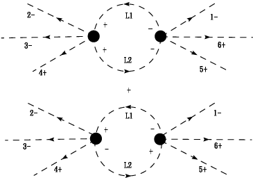
Figure 1: Here we show for a particular case of the gluonic NMHV loop amplitude, different assignment of helicity for the propagators will change the MHV or $\overline{MHV}$ nature of each vertex. In the upper graph the propagators has the same helicity on each vertex while in the lower they are opposite. This result in a MHV vertex on the left for the upper graph and an $\overline{MHV}$ vertex on the left for the lower graph. In practice one has to sum these two possibilities which is the reason we have two terms in eq.(5)-(7)

$$g_{i}^{-}=\eta^{1}_{i}\eta^{2}_{i}\eta^{3}_{i}\eta^{4}_{i},\;\phi^{AB}_{i}=\eta^{A}_{i}\eta^{B}_{i},\;\Lambda^{1-}_{i}=-\eta^{2}_{i}\eta^{3}_{i}\eta^{4}_{i},\;\Lambda^{2-}_{i}=-\eta^{1}_{i}\eta^{3}_{i}\eta^{4}_{i}$$ (10)

$$\qquad\Lambda^{3-}_{i}=-\eta^{1}_{i}\eta^{2}_{i}\eta^{4}_{i},\qquad\Lambda^{4-}_{i}=-\eta^{1}_{i}\eta^{2}_{i}\eta^{3}_{i},\qquad\Lambda^{A+}_{i}=\eta^{A}_{i},\qquad g_{i}^{+}=1$$

The superscript represents which flavor the particle carries, in the N=4 multiplet there are four gluinos and six scalars. Corresponding combination in the $\widetilde{\eta}$ follows:

$$g_{i}^{+}=\widetilde{\eta^{1}_{i}}\widetilde{\eta^{2}_{i}}\widetilde{\eta^{3}_{i}}\widetilde{\eta^{4}_{i}},\;\phi^{AB}_{i}=\widetilde{\eta^{C}_{i}}\widetilde{\eta^{C}_{i}},\;\Lambda^{1+}_{i}=-\widetilde{\eta^{2}_{i}}\widetilde{\eta^{3}_{i}}\widetilde{\eta^{4}_{i}},\;\Lambda^{2+}_{i}=-\widetilde{\eta^{1}_{i}}\widetilde{\eta^{3}_{i}}\widetilde{\eta^{4}_{i}}$$ (11)

$$\qquad\Lambda^{3+}_{i}=-\widetilde{\eta^{1}_{i}}\widetilde{\eta^{2}_{i}}\widetilde{\eta^{4}_{i}},\qquad\Lambda^{4+}_{i}=-\widetilde{\eta^{1}_{i}}\widetilde{\eta^{2}_{i}}\widetilde{\eta^{3}_{i}},\qquad\Lambda^{A-}_{i}=\widetilde{\eta^{A}_{i}},\qquad g^{-}_{i}=1$$

Thus a particular term in the expansion corresponds to a particular assignment of the fermionic variables to the external particle and results in an amplitude with a particular set of external particle specie and helicity ordering. In the next two section we show by expanding eq.(5),(6),(7) and following the above dictionary one can recover the amplitudes containing two same color gluino with different helicity ordering computed in 5 .

II.1 2.1 $B_{1}$ Coefficient $\Rightarrow$ $t_{123}$ cut

First we look at the $t_{123}$ cut which correspond to the $B_{1}$ coefficient. For the purely gluonic amplitude $A(g_{1}^{-}g_{2}^{-}g_{3}^{-}|g_{4}^{+}g_{5}^{+}g_{6}^{+})$ (we use a bar to indicate the cut ), we have only one particle assignment for the loop propagators:

$$l_{1}=g^{+}\;,l_{2}=g^{+}$$ (12)

Here the assignment of helicity is labelled with respect to the $\overline{MHV}$ vertex. Therefore we get only contribution from the first term in eq.(5), the expansion from the delta function gives $\langle\l_{1}l_{2}\rangle^{4}[l_{1}l_{2}]^{4}=(l_{1}-l_{2})^{8}=t_{123}^{4}$ and therefore $B_{1}=t_{123}^{3}B_{0}$ which matches eq.(5.4) in 5 .

For the two gluino amplitudes first we look at $A(\Lambda^{-}_{1}g_{2}^{-}g_{3}^{-}|\Lambda^{+}_{4}g_{5}^{+}g_{6}^{+})$ from the delta function expansion the we have helicity assignments :

$$l_{1}=\Lambda^{+}\;l_{2}=g^{+}\;,\;+(\;exchage\;between\;l_{1}\;and\;l_{2}\;)$$ (13)

Again only the first term in eq.(5) gives contribution :

$$\langle l_{1}l_{2}\rangle^{3}[l_{1}l_{2}]^{3}([1l_{1}]\langle l_{1}4\rangle-[1l_{2}]\langle l_{2}4\rangle)=t_{123}^{3}\langle 1|K_{123}|4\rangle$$ (14)

Note that only when the external gluino carry the same flavor will this term contribute. Since in 5 the two gluino amplitude was derived using N=1 SWI, the two gluinos carry the same flavor. Thus we have

$$B_{1}(\Lambda^{-}_{1}g_{2}^{-}g_{3}^{-}|\Lambda^{+}_{4}g_{5}^{+}g_{6}^{+})=i\frac{t_{123}^{2}\langle 1|K_{123}|4\rangle}{[12][23]<45><56><1|K_{123}|4><3|K_{123}|6>}$$ (15)

This is exactly the result of 5 . Other non-cyclic permutations of two gluino amplitude calculated in 5 at this cut do not change the assignment of the propagators thus the amplitude remains the same form apart from the labelling of the position of the two gluinos.

II.2 2.2 $B_{2}$ Coefficient $\Rightarrow$$t_{234}$ cut

For this cut with different helicity assignment of the propagators, contribution can arise from both terms. Propagators with the same helicities (here we mean they are both plus or minus regardless of the specie) get its contribution from one term while the rest from the other, this is why $B_{2}$ was split in two terms in the original computation of the gluon amplitude 2 . We deal with the same helicity first since there is only one way of assigning propagators.

$B_{2}(\Lambda^{-}_{1}|g_{2}^{-}g_{3}^{-}\Lambda^{+}_{4}|g_{5}^{+}g_{6}^{+})_{samehelicity}=0$ since there is no way of assigning same helicity particles to the propagators.

For $B_{2}(g_{1}^{-}|\Lambda^{-}_{2}g_{3}^{-}\Lambda^{+}_{4}|g_{5}^{+}g_{6}^{+})_{samehelicity}$ we have

$$l_{1}=g^{-}\;l_{2}=g^{-}$$ (16)

this receives contribution from the second term in eq.(6) which is $\langle 23\rangle^{3}\langle 43\rangle[56]^{4}$ thus giving

$$B_{2}(g_{1}^{-}|\Lambda^{-}_{2}g_{3}^{-}\Lambda^{+}_{4}|g_{5}^{+}g_{6}^{+})_{samehelicity}=(\frac{\langle 23\rangle^{3}\langle 43\rangle[56]^{4}}{t_{234}})B_{+}^{{\dagger}}$$ (17)

For $B_{2}(g_{1}^{-}|\Lambda^{-}_{2}g_{3}^{-}g_{4}^{+}|\Lambda^{+}_{5}g_{6}^{+})_{samehelicity}$ we have

$$l_{1}=g^{-}\;l_{2}=\Lambda^{-}\;,+\;(exchange\;between\;l_{1},l_{2})$$ (18)

This gives contribution $\langle 23\rangle^{3}[56]^{3}(\langle 3l_{1}\rangle[l_{1}6]-\langle 3l_{2}\rangle[l_{2}6])=\langle 23\rangle^{3}[56]^{3}\langle 3|K_{234}|6\rangle$ giving

$$B_{2}(g_{1}^{-}|\Lambda^{-}_{2}g_{3}^{-}g_{4}^{+}|\Lambda^{+}_{5}g_{6}^{+})_{samehelicity}=(\frac{\langle 23\rangle^{3}[56]^{3}\langle 3|K_{234}|6\rangle}{t_{234}})B_{+}^{{\dagger}}$$ (19)

Now we move to configurations with different helicity. For $B_{2}(\Lambda^{-}_{1}|g_{2}^{-}g_{3}^{-}\Lambda^{+}_{4}|g_{5}^{+}g_{6}^{+})_{DiffHelicity}$ we have :

$$l_{1}=\Lambda^{+}\;l_{2}=g^{-}\;,l_{1}=\Lambda^{-}\;l_{2}=\phi\;,+\;(exchange\;between\;l_{1},l_{2})$$ (20)

For fix flavored $\Lambda_{4}^{+}$ and $\Lambda_{1}^{-}$ we have to sum up all possible flavors for the internal gluino. This gives a contribution of

$$[1l_{1}]^{3}[l_{1}l_{2}]\langle 4l_{2}\rangle^{3}\langle l_{1}l_{2}\rangle-3[l_{1}l_{2}][l_{2}4][l_{1}4]^{2}\langle l_{1}l_{2}\rangle\langle l_{2}1\rangle\langle l_{1}1\rangle^{2}$$ (21)

$$+3[l_{1}l_{2}][l_{1}4][l_{2}4]^{2}\langle l_{1}l_{2}\rangle\langle l_{1}1\rangle\langle l_{2}1\rangle^{2}$$

$$-[1l_{2}]^{3}[l_{1}l_{2}]\langle 4l_{2}\rangle^{3}\langle l_{1}l_{2}\rangle=t_{123}(\langle 1|l_{1}-l_{2}|4\rangle)^{3}=t_{123}\langle 1|K_{123}|4\rangle^{3}$$

Therefore

$$B_{2}(\Lambda^{-}_{1}|g_{2}^{-}g_{3}^{-}\Lambda^{+}_{4}|g_{5}^{+}g_{6}^{+})_{DiffHelicity}=\frac{\langle 1|K_{123}|4\rangle^{3}}{t_{123}^{3}}B_{+}$$ (22)

For $B_{2}(g_{1}^{-}|\Lambda^{-}_{2}g_{3}^{-}\Lambda^{+}_{4}|g_{5}^{+}g_{6}^{+})_{DiffHelicity}$ we have:

$$l_{1}=g^{-}\;l_{2}=g^{+}\;,l_{1}=\Lambda^{+}\;l_{2}=\Lambda^{-}\;,l_{1}=\phi\;l_{2}=\phi\;,\;+\;(exchange\;between\;l_{1},l_{2})$$ (23)

Here whether or not $\Lambda_{4}^{+}$ and $\Lambda_{1}^{-}$ carry the same flavor will effect the number of ways one can assign flavor to the internal gluino and scalar. For the same flavor we have

$$-([4l_{1}]\langle l_{1}1\rangle-[4l_{2}]\langle l_{2}1\rangle)^{3}([2l_{1}]\langle l_{1}1\rangle-[2l_{2}]\langle l_{2}1\rangle)=-(\langle 4|K_{234}|1\rangle)^{3}(\langle 2|K_{234}|1\rangle)$$ (24)

Thus

$$B_{2}(g_{1}^{-}|\Lambda^{-}_{2}g_{3}^{-}\Lambda^{+}_{4}|g_{5}^{+}g_{6}^{+})_{DiffHelicity}=(\frac{-(\langle 4|K_{234}|1\rangle)^{3}(\langle 2|K_{234}|1\rangle)}{t_{234}})B_{+}$$ (25)

For $B_{2}(g^{-}_{1}|\Lambda_{2}^{-}g_{3}^{-}g_{4}^{+}|\Lambda^{+}_{4}g^{+}_{6})_{Diffhelicity}$ we have :

$$l_{1}=g^{-}\;l_{2}=\Lambda^{+}\;,l_{1}=\Lambda^{-}\;l_{2}=\phi\;,\;+\;(exchange\;between\;l_{1},l_{2})$$ (26)

This gives contribution :

$$-\langle 1l_{1}\rangle^{3}\langle 15\rangle[l_{1}4]^{3}[42]+3\langle 1l_{1}\rangle^{2}[l_{1}4]^{2}\langle 1l_{2}\rangle[l_{2}4][42]\langle 15\rangle$$ (27)

$$-3\langle 1l_{2}\rangle^{2}[l_{2}4]^{2}\langle 1l_{1}\rangle[l_{1}4][42]\langle 15\rangle+\langle 1l_{1}\rangle^{3}\langle 15\rangle[l_{1}4]^{3}[42]$$

$$=-(\langle 4|K_{234}|1\rangle)^{3}[42]\langle 15\rangle$$

Thus

$$B_{2}(g^{-}_{1}|\Lambda_{2}^{-}g_{3}^{-}g_{4}^{+}|\Lambda^{+}_{4}g^{+}_{6})_{Diffhelicity}=\frac{-(\langle 4|K_{234}|1\rangle)^{3}[42]\langle 15\rangle}{t_{234}}B_{+}$$ (28)

Adding eq.(17),(19),(22),(25) and (28) together gives the $B_{2}$ coefficient of the gluino anti-gluino pair amplitudes computed in 5 . Coefficients for the next cut can be calculated in similar way, we’ve checked it gives the same result as that derived in 5 .

It is straight forward to compute amplitudes that involve more than one pair of gluino or scalar. The new amplitudes are :

$$A(g^{-}g^{+}\Lambda^{+}\Lambda^{-}\Lambda^{-}\Lambda^{+})\;,A(g^{-}g^{+}\phi\phi\phi\phi)\;,A(\phi\phi\phi\phi\phi\phi)\;A(\Lambda^{-}\Lambda^{-}\Lambda^{-}\Lambda^{+}\Lambda^{+}\Lambda^{+})\;,$$ (29)

$$A(\Lambda^{-}\Lambda^{+}\phi\phi\phi\phi)\;,A(\Lambda^{-}\Lambda^{-}\Lambda^{+}\Lambda^{+}\phi\phi)\;,A(\Lambda^{-}\Lambda^{+}\phi g^{-}g^{+}g^{+})$$

Complication arises for these amplitudes because non-gluon particles carry less superspace variables and increase the amount of spinor combination. Luckily with the specification of the flavor for the external particles, the propagators are restricted to take certain species. This is discussed in detail in the next section where we calculate the all gluino and all scalar amplitude.

III 3. Amplitudes with all gluinos and all scalars

Here we present N=4 SYM NMHV loop amplitudes with all gluino and all scalars. These amplitudes were derived from explicit expansion of eq.(5)-(7). Since scalars and gluinos carry less fermionic parameters as seen in eq.(10)(11), the spinor product that arises from the fermionic delta function becomes complicated. The final coefficient should not contain the off shell propagator spinor, thus one can use this as a guideline to group the spinor products to form kinematic invariant terms. With specific flavors this also restrict the possible species for propagators.

III.1 3.1 $A(\Lambda_{1}^{\emph{1}+}\Lambda_{2}^{\emph{2}+}\Lambda_{3}^{\emph{3}+}\Lambda_{4}^{\emph{1}-}\Lambda_{5}^{\emph{2}-}\Lambda_{6}^{\emph{3}-})$

For the six gluino amplitude we look at amplitudes with all three positive helicity gluino carrying different flavor. The negative helicities also carry different flavor and is the same set as the positive. For $t_{123}$ the flavors of the internal particles are uniquely determined.

$$l_{1}=\Lambda^{-}\;l_{2}=g^{+}\;,\;l_{1}=\Lambda^{+}\;l_{2}=\phi\;,\;+exchange$$ (30)

This gives

$$B_{1}(\Lambda_{1}^{\emph{1}+}\Lambda_{2}^{\emph{2}+}\Lambda_{3}^{\emph{3}+}|\Lambda_{4}^{\emph{1}-}\Lambda_{5}^{\emph{2}-}\Lambda_{6}^{\emph{3}-})=(\langle 1|K_{123}|5\rangle\langle 2|K_{123}|6\rangle\langle 3|K_{123}|4\rangle$$ (31)

$$+\langle 1|K_{123}|4\rangle\langle 2|K_{123}|5\rangle\langle 3|K_{123}|6\rangle+\langle 1|K_{123}|6\rangle\langle 2|K_{123}|4\rangle\langle 3|K_{123}|5\rangle)B_{0}^{{\dagger}}$$

Next we look at $t_{345}$ cut. The propagator assignment with same helicity (the definition of same or different helicity again follows that of the previous paragraph ) would be :

$$l_{1}=g^{-}\;l_{2}=\Lambda^{-}\;,\;+exchange\;propagator$$ (32)

this gives

$$B_{3}(\Lambda_{1}^{\emph{1}+}\Lambda_{2}^{\emph{2}+}|\Lambda_{3}^{\emph{\emph{3}}+}\Lambda_{4}^{\emph{1}-}\Lambda_{5}^{\emph{2}-}|\Lambda_{6}^{\emph{3}-})_{SameHelicity}=\langle 45\rangle^{2}[12]^{2}\{\langle 34\rangle[61]\langle 5|K_{345}|2\rangle$$ (33)

$$+\langle 34\rangle[62]\langle 5|K_{345}|1\rangle+\langle 35\rangle[61]\langle 4|K_{345}|2\rangle+\langle 35\rangle[62]\langle 4|K_{345}|1\rangle\}B_{-}^{{\dagger}}$$

There are two ways of assigning different helicity propagators

$$l_{1}=g^{-}\;l_{2}=\Lambda^{+}\;,\;orl_{1}=\Lambda^{-}\;l_{2}=\phi\;,\;+\;exchange$$ (34)

Note however for the present set of flavors, there is no consistent way of assigning flavors when the propagators are a gluon and a gluino. Thus we are left with the gluino scalar possibility with it’s flavor uniquely determined.

$$B_{3}(\Lambda_{1}^{\emph{1}+}\Lambda_{2}^{\emph{2}+}|\Lambda_{3}^{\emph{3}+}\Lambda_{4}^{\emph{1}-}\Lambda_{5}^{\emph{2}-}|\Lambda_{6}^{\emph{3}-})_{DiffHelicity}=\langle 16\rangle\langle 62\rangle[43][35]\langle 6|K_{345}|3\rangle t_{345}B_{-}$$ (35)

Luckily there is no need to compute $B_{2}$ coefficients since it is related to $B_{3}$ by symmetry.

III.2 3.2 $A(\phi_{1}\phi_{2}\phi_{3}\phi_{4}\phi_{5}\phi_{6})$

The power of deriving amplitudes from a superspace expansion is that one can rule out certain amplitudes just by inspection. Amplitudes with more than two scalars carrying the same color vanishes since there is no way of assigning the correct fermionic variables. Here we look at six scalar amplitude all carrying different flavor. This should be the simplest amplitude since the flavor carried by the internal particle is uniquely determined. We give the result for cut $t_{123}$ while the other cuts are related by symmetry.

$$B_{1}(\phi_{1}\phi_{2}\phi_{3}\phi_{4}\phi_{5}\phi_{6})=\{(\langle 12\rangle[56]\langle 3|K_{123}|4\rangle+\langle 12\rangle[64]\langle 3|K_{123}|5\rangle+\langle 12\rangle[45]\langle 3|K_{123}|6\rangle$$ (36)

$$+\langle 31\rangle[56]\langle 2|K_{123}|4\rangle+\langle 31\rangle[64]\langle 2|K_{123}|5\rangle+\langle 31\rangle[45]\langle 2|K_{123}|6\rangle$$

$$+\langle 23\rangle[56]\langle 1|K_{123}|4\rangle+\langle 23\rangle[64]\langle 1|K_{123}|5\rangle+\langle 23\rangle[45]\langle 1|K_{123}|6\rangle)^{2}\}B_{0}$$

$$+complex\;conjugate.$$

IV 4. A brief discussion on the MHV vertex approach

As discussed in the introduction, the straight forward way to compute amplitudes in superspace is the generalization of the MHV vertex 10 approach. It is also of conceptual interest to see if this approach actually works for the NMHV loop amplitude. Here we give a brief discussion of the extension.

The MHV vertex approach was shown to be successful 12 in constructing the n point MHV loop amplitude. This is partly due to the similarity between the cut diagrams 1 originally used to compute the amplitude and the MHV vertex diagram, so that one can use a dispersion type integral to reconstruct the box functions from it’s discontinuity across the branch cut. For the NMHV loop amplitude, one requires three propagator for the three MHV vertex one-particle-irreducible(1PI) diagram and two propagators for the one-particle-reducible(1PR) diagram (fig-2)13 .

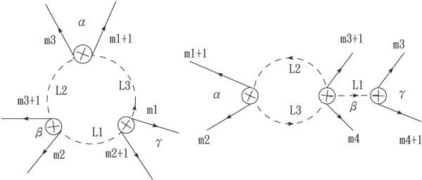
Figure 2: MHV diagrams for NMHV loop amplitude, includes the one-particle-irreducible and one-particle-reducible graph. The $m_{i}$s label external momenta that are adjacent to the propagator. For the first graph we need to integrate over all three propagators, while only $L_{2}$ $L_{3}$ are integrated in the second. One also needs to sum over all possible ways of assigning external momenta to the vertices

We would then encounter the following integration:

$$\frac{1}{\prod_{i=1}^{n}\langle ii+1\rangle}\int\frac{d^{4}L_{1}}{L_{1}^{2}}\frac{d^{4}L_{2}}{L_{2}^{2}}\frac{d^{4}L_{3}}{L_{3}^{2}}\delta(P_{\alpha}+L_{2}-L_{3})\delta(P_{\beta}+L_{3}-L_{1})\delta(P_{\gamma}+L_{1}-L_{2})$$ (37)

$$\int d^{8}\eta_{l_{1}}d^{8}\eta_{l_{2}}d^{8}\eta_{l_{3}}\frac{\delta^{8}(\Theta_{1})\delta^{8}(\Theta_{2})\delta^{8}(\Theta_{3})\langle m_{2}m_{2}+1\rangle\langle m_{1}m_{1}+1\rangle\langle m_{3}m_{3}+1\rangle}{\langle l_{2}l_{1}\rangle\langle l_{3}l_{2}\rangle\langle l_{1}l_{3}\rangle\langle l_{1}m_{2}+1\rangle\langle m_{2}l_{1}\rangle\langle l_{2}m_{3}+1\rangle\langle m_{3}l_{2}\rangle\langle l_{3}m_{1}+1\rangle\langle m_{1}l_{3}\rangle}$$

$$+\frac{\delta(L_{1}-P_{\gamma})}{\prod_{i=1}^{n}\langle ii+1\rangle}\int\frac{d^{4}L_{2}}{L_{2}^{2}}\frac{d^{4}L_{3}}{L_{3}^{2}}\delta(P_{\alpha}+L_{3}-L_{2})\delta(P_{\beta}+L_{2}+L_{1}-L_{3})\int d^{8}\eta_{l_{1}}d^{8}\eta_{l_{2}}d^{8}\eta_{l_{3}}$$

$$\times\frac{\delta^{8}(\Theta_{1})\delta^{8}(\Theta_{2})\delta^{8}(\Theta_{3})\langle m_{2}m_{2}+1\rangle\langle m_{1}m_{1}+1\rangle\langle m_{3}m_{3}+1\rangle\langle m_{4}m_{4}+1\rangle}{L_{1}^{2}\langle l_{3}l_{2}\rangle^{2}\langle m_{1}l_{2}\rangle\langle l_{2}m_{1+1}\rangle\langle l_{3}m_{2}+1\rangle\langle m_{2}l_{3}\rangle\langle l_{1}m_{3}+1\rangle\langle m_{3}l_{1}\rangle\langle l_{1}m_{4}+1\rangle\langle m_{4}l_{1}\rangle}$$

where for the first term

$$\Theta_{1}=\sum_{i=\alpha}\eta_{i}\lambda_{i}+l_{2}\eta_{l_{2}}-l_{3}\eta_{l_{3}}$$ (38)

$$\Theta_{2}=\sum_{i=\beta}\eta_{i}\lambda_{i}+l_{3}\eta_{l_{3}}-l_{1}\eta_{l_{1}}$$

$$\Theta_{3}=\sum_{i=\gamma}\eta_{i}\lambda_{i}+l_{1}\eta_{l_{1}}-l_{2}\eta_{l_{2}}$$

for the second term

$$\Theta_{1}=\sum_{i=\alpha}\eta_{i}\lambda_{i}-l_{2}\eta_{l_{2}}+l_{3}\eta_{l_{3}}$$ (39)

$$\Theta_{2}=\sum_{i=\beta}\eta_{i}\lambda_{i}+l_{1}\eta_{l_{1}}+l_{2}\eta_{l_{2}}-l_{3}\eta_{l_{3}}$$

$$\Theta_{3}=\sum_{i=\gamma}\eta_{i}\lambda_{i}-l_{1}\eta_{l_{1}}$$

$\alpha$$\beta$$\gamma$ labels the external momenta assigned to the three MHV vertex and the $l_{i}$s are the off shell continuation spinor following the CSW prescription 10 . We can reorganize the delta functions to reproduce the overall momentum conservation. For the first term in eq.(37) we have

$$\delta(P_{\alpha+\beta+\gamma})\delta(P_{\beta+\gamma}+L_{3}-L_{2})\delta(P_{\gamma}+L_{1}-L_{2})$$ (40)

For the second term

$$\delta(P_{\alpha+\beta+\gamma})\delta(P_{\alpha}+L_{2}-L_{3})$$

If we integrate the last delta function away in the first term and combine with the 1PR graphs, it is equivalent to using two MHV vertex to construct NMHV tree amplitude on one side of the two remaining propagator, namely this combines vertex $\gamma$ and $\beta$ through propagator $L_{1}$. To see this note that the momentum conserving delta function forces $L_{1}$ propagator to carry the correct momentum as it would for the CSW method and the $\frac{1}{P_{L_{1}}^{2}}$ is present in the integral measure in the first place. This would obviously affect the off shell spinor in the following way.

$$l_{1}=L_{1}\widetilde{\eta}\rightarrow(L_{2}-P_{\gamma})\widetilde{\eta}$$ (41)

This simply fixes the off shell spinor to be computed from the correct momentum as the CSW method. Thus we have come to a two propagator integral with two tree level amplitude on both side constructed from the CSW method. This is exactly the picture one would have if one apply the standard cut, except the propagators are off shell instead of on shell. For higher number of MHV vertices this can be applied straight forward, by integrating the momentum conserving propagator one at a time one can reduce the number of propagators until one arrive at the standard cut picture. As shown in 12 one can then proceed to recast the two propagator integral into a dispersion integral which computes the discontinuity across the cut of the integrand, by using the cut constructibility of N=4 SYM loop amplitudes, one can reconstruct the box function and it’s coefficient. However there is one subtlety. In the original standard cut one has to analyze every cut channel, and then disentangle the information since more than one box integral share the same cuts. If we follow the CSW prescription we can always reduce the loop diagrams down to two propagator one loop diagrams with a MHV vertex on one side of the two propagators. Thus this implies if the CSW approach is valid at one loop, then the full loop amplitude should be able to be reconstructed from the cuts of a subgroup of two propagator diagrams which always have a MHV vertex on one side of the cut.

This construction makes the connection between MHV vertex and $\overline{MHV}$ loop amplitude more transparent. $\overline{MHV}$ loop are just the parity transformation of the MHV loop, where one simply take the complex conjugate of the MHV loop:

$$A(\overline{MHV})_{loop}=A(\overline{MHV})_{tree}\sum_{i=1}^{n}\sum_{r=1}^{[n/2]-1}(1-\frac{1}{2}\delta_{\frac{n}{2}},r)F^{2me}_{n:r;i}$$ (42)

It’s derivation from MHV vertex is as follows. In 15 it was shown that using MHV vertices one can reconstruct the $\overline{MHV}$ tree amplitude in it’s complex conjugate spinor form. Since by integrating out one loop propagator corresponds to using MHV vertex to construct NMHV tree amplitude, one can proceed in a specific manner to reduce the number of loop propagators down to two with two $\overline{MHV}$ tree on both side. Since from 15 the two $\overline{MHV}$ tree amplitudes on both side is expressed in complex conjugate form, following exactly the same lines in 12 one can reproduce eq.(43).

V 5. Conclusion

In this paper we constructed the 6 point NMHV loop amplitude for N=4 SuperYang-Mills in a compact form using its cut constructible nature. The expansion with respect to the fermionic parameter gives amplitudes with different particle content and helicity ordering. To extend further to higher point NMHV loops one may have to resolve to the MHV vertex approach since the tree level amplitudes on both side of the cut in general will not be in simple MHV and $\overline{MHV}$ combination. We also give a general discussion on how to proceed with the MHV vertex construction for higher than MHV loop(more than two negative helicities). The fact that it reproduces the two propagator picture for any one loop diagram combined with earlier results that have reproduced the MHV loop12 and the relationship between the leading order and sub leading order amplitudes13 , gives a strong support for the CSW approach beyond tree level.

VI 6. Acknowledgements

It is a great pleasure to thank Warren Siegel for suggesting the question, Gabriele Travaglini, L. J. Dixon and Freddy Cachazo for their useful comments.

References

- (1) Z. Bern, L. J. Dixon, D. C. Dunbar and D. A. Kosower, Nucl. Phys. B 425, 217 (1994) [arXiv:hep-ph/9403226].
- (2) Z. Bern, L. J. Dixon, D. C. Dunbar and D. A. Kosower, Nucl. Phys. B 435, 59 (1995) [arXiv:hep-ph/9409265].
- (3) R. Britto, F. Cachazo and B. Feng, arXiv:hep-th/0412103.
- (4) Z. Bern, L. J. Dixon and D. A. Kosower, Nucl. Phys. B 513, 3 (1998) [arXiv:hep-ph/9708239]. Z. Bern, L. J. Dixon and D. A. Kosower, JHEP 0408, 012 (2004) [arXiv:hep-ph/0404293]. Z. Bern, V. Del Duca, L. J. Dixon and D. A. Kosower, Phys. Rev. D 71, 045006 (2005) [arXiv:hep-th/0410224].
- (5) S. J. Bidder, D. C. Dunbar and W. B. Perkins, arXiv:hep-th/0505249.
- (6) M. T. Grisaru, H. N. Pendleton and P. van Nieuwenhuizen, Phys. Rev. D 15, 996 (1977).
- (7) V. P. Nair, Phys. Lett. B 214, 215 (1988).
- (8) E. Witten, Commun. Math. Phys. 252, 189 (2004) [arXiv:hep-th/0312171].
- (9) R. Britto, F. Cachazo and B. Feng, Nucl. Phys. B 715, 499 (2005) [arXiv:hep-th/0412308]. R. Britto, B. Feng, R. Roiban, M. Spradlin and A. Volovich, Phys. Rev. D 71, 105017 (2005) [arXiv:hep-th/0503198]. R. Britto, F. Cachazo, B. Feng and E. Witten, Phys. Rev. Lett. 94, 181602 (2005) [arXiv:hep-th/0501052].
- (10) F. Cachazo, P. Svrcek and E. Witten, JHEP 0409, 006 (2004) [arXiv:hep-th/0403047].
- (11) G. Georgiou, E. W. N. Glover and V. V. Khoze, JHEP 0407, 048 (2004) [arXiv:hep-th/0407027].
- (12) A. Brandhuber, B. Spence and G. Travaglini, Nucl. Phys. B 706, 150 (2005) [arXiv:hep-th/0407214].
- (13) M. x. Luo and C. k. Wen, Phys. Lett. B 609, 86 (2005) [arXiv:hep-th/0410118]. M. x. Luo and C. k. Wen, JHEP 0411, 004 (2004) [arXiv:hep-th/0410045].
- (14) G. Georgiou, E. W. N. Glover and V. V. Khoze, JHEP 0407, 048 (2004) [arXiv:hep-th/0407027].
- (15) J. B. Wu and C. J. Zhu, JHEP 0407, 032 (2004) [arXiv:hep-th/0406085]. J. B. Wu and C. J. Zhu, JHEP 0409, 063 (2004) [arXiv:hep-th/0406146].