Also at ]Landau Institute of Theoretical Physics.

Harmonic measure of critical curves

Abstract

Fractal geometry of critical curves appearing in 2D critical systems is characterized by their harmonic measure. For systems described by conformal field theories with central charge $c\leqslant 1$, scaling exponents of the harmonic measure have been computed by B. Duplantier [Phys. Rev. Lett. 84, 1363 (2000)] by relating the problem to boundary two-dimensional gravity. We present a simple argument connecting the harmonic measure of critical curves to operators obtained by fusion of primary fields, and compute characteristics of the fractal geometry by means of regular methods of conformal field theory. The method is not limited to theories with $c\leqslant 1$.

Introduction.

Two-dimensional (2D) statistical models typically exhibit stochastic curves, such as external perimeters of critical clusters in the Potts model or fluctuating loops in models of Refs. [nienhuis, –kondevhenley, ]. In the critical regime these curves are fractal. Different phases of loop models exhibit two distinct types of critical curves: dilute and dense. Dilute curves are simple while dense curves have infinitely many double points at which they touch but do not intersect. There exists a duality relation between the two types, in particular, the external perimeter of a dense curve is a dilute curve duplantier . Despite of a long history of studying critical phenomena, inquiries into the stochastic geometry of the critical curves are relatively recent. Traditional conformal field theory (CFT) cft concentrates on correlations of local fields and essentially leaves their relation to geometrical objects, such as critical curves, unclear. B. Duplantier, in a seminal paper duplantier , found the harmonic multifractal spectrum of critical curves arising in critical systems with the central charge $c\leqslant 1$ (see Eqs. (9, 8)). His method used an intriguing connection between CFT and 2D boundary quantum gravity. More recently, the stochastic Loewner evolution approach was successfully used for the same purpose slepeople . Both methods are interesting and powerful, but somewhat foreign to traditional CFT approach and not obviously susceptible to generalizations.

In this letter we show that geometrical properties of dilute critical curves are naturally linked to correlation functions of primary fields and can be studied within the regular framework of CFT, not limited to theories with $c\leqslant 1$. Our arguments may also shed some light on the boundary quantum gravity itself.

Harmonic measure of critical curves.

A basic characteristic of simple curves is the harmonic measure ahlfors . It has a simple electrostatic interpretation. Consider a closed curve $\gamma$ made of a conducting material and carrying a total electric charge of one. Harmonic measure of any part of the curve is the charge of this part. In what follows we will pick a point of interest $z_{0}$ on the curve and consider a disc of a small radius $r$ centered at $z_{0}$ as is in the Figure. It surrounds a small part of the curve, and we define $\mu(r)$ to be harmonic measure of this part.

If a curve is a closed loop lying entirely in the bulk (i.e. it does not touch the system boundaries), all its points are statistically identical. We can also consider the case when a curve emerges from a boundary, and the case when a curve has one or both dangling ends in the bulk. The latter is achieved by inserting into the system a small isolated boundary (almost a puncture) so that the curve ends on this boundary. Statistics of harmonic measure is different in the following three cases duplantier depicted in the Figure: (i) bulk, if $z_{0}$ lies in the bulk and is not an endpoint; (ii) boundary, if $z_{0}$ is a point where $\gamma$ is connected with the system boundary; (iii) extremity, if $z_{0}$ is a dangling endpoint of $\gamma$ in the bulk. More generally one may consider $n$ curves emanating from the boundary, or $n$ curves meeting at a point in the bulk. The bulk and extremity cases correspond to $n=2$ and $n=1$.

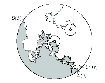
Figure 1: Harmonic measure of a critical curve evaluated in the bulk, on the system boundary, and at an extremity.

Let us define a conformal map $w(z)$ of the exterior of $\gamma$ to some standard domain. For a closed loop in the bulk it can be the exterior of a unit disc, while for a curve with both ends on the system boundary or a “sprout”, the upper half plane is more convenient. We normalize the map so that the point of interest $z_{0}$ is mapped onto itself, choose it to be the origin $z_{0}=0$, $w(0)=0$, and demand that $w^{\prime}(\infty)=1$. The moments of harmonic measure of dilute critical curves scale at small $r$ with non-trivial exponents. The relations $\mu(r)\sim|w(r)|\sim r|w^{\prime}(r)|$ follow from the definition of $\mu(r)$. Therefore, the scaling of the moments of $\mu(r)$ is determined by that of $|w^{\prime}(r)|$:

$$\prec\!\!|w^{\prime}(r)|^{h}\!\!\succ\;\sim\;r^{\Delta(h)},\quad r\rightarrow 0.$$ (1)

The notation $\prec\!\!\dots\!\!\succ$ stands for statistical average over the ensemble of critical curves. The notation $\langle\dots\rangle$ is reserved for correlators of CFT.

Harmonic measure and fluctuating geometry.

The scaling of the harmonic measure may be computed by considering CFT correlation functions. It is the easiest to start with a point where a curve $\gamma$ connects with the system boundary. We assume that the system occupies the interior of an annulus. The curve starts from the large circle at $z_{0}=0$, ending on the large circle at a point $L$.

The partition function $Z(0,L)$ restricted to configurations that contain a curve $\gamma$ connecting the points 0 and $L$, is given by the correlator of two appropriate boundary operators $\mathcal{B}$ changing boundary conditions cardyoperators . These operators create curves emanating from the boundary duplantiersaleur :

$$Z(0,L)/Z=\langle\mathcal{B}(0)\mathcal{B}(L)\rangle_{\mathbb{H}},$$ (2)

where $Z$ is the unrestricted partition function. The subscript of $\langle\dots\rangle$ refers to the domain of definition, in this case the upper half plane.

This correlator, as indeed any correlator containing two boundary operators $\mathcal{B}$, can be computed in two steps: In the first step we pick a particular realization of the curve $\gamma$. Within each realization, the curve $\gamma$ is the boundary separating two independent systems—the interior and the exterior of $\gamma$—with partition functions $Z^{\mathrm{int}}_{\gamma}$ and $Z^{\mathrm{ext}}_{\gamma}$, respectively. These are stochastic objects that depend on the fluctuating geometry of $\gamma$. At the second step we sum over the realizations of $\gamma$. We thus obtain

$$Z(0,L)=\prec\!\!Z^{\mathrm{int}}_{\gamma}Z^{\mathrm{ext}}_{\gamma}\!\!\succ.$$ (3)

We further insert an additional boundary primary operator $O_{h}(r)$ of conformal weight $h$ sufficiently close to 0, and a second copy $O_{h}(\infty)$. Both act as a source of harmonic measure. We thus consider the correlator

$$\langle O_{h}(r)\mathcal{B}(0)\mathcal{B}(L)O_{h}(\infty)\rangle_{\mathbb{H}}.$$ (4)

Since we are only interested in the $r$-dependence of the correlator, we can fuse together the distant primary fields: $\mathcal{B}(L)\times O_{h}(\infty)=\Psi(\infty)$. We therefore consider the $r$-dependence of a 3-point function

$$\langle O_{h}(r)\mathcal{B}(0)\Psi(\infty)\rangle_{\mathbb{H}},$$ (5)

and show that it yields the statistics of the harmonic measure.

Decomposing the upper half plane into the exterior and the interior of $\gamma$ as before, we can rewrite (4) as the average over the fluctuating geometry of $\gamma$:

$$\prec\!\!\langle O_{h}(r)O_{h}(\infty)\rangle^{\mathrm{ext}}_{\gamma}Z^{\mathrm{int}}_{\gamma}Z^{\mathrm{ext}}_{\gamma}\!\!\succ/Z$$ (6)

Here the domain of the definition of the correlator of primary fields is the exterior of $\gamma$. This correlator is statistically independent from the other two factors in the numerator of (6) in the limit $r\ll|L|$. We are left with the correlation function $\langle O_{h}(r)O_{h}(\infty)\rangle^{\mathrm{ext}}_{\gamma}$ of two primary fields of boundary CFT, further averaged over all configuration of the boundary $\gamma$. It is equal to the 3-point correlation function (5).

Now we apply the conformal transformation $w(z)$ which maps the exterior of $\gamma$ onto the upper half plane. Being a primary operator of conformal weight $h$, $O_{h}(r)$ transforms as $O_{h}\rightarrow O_{h}(w(r))|w^{\prime}(r)|^{h}$, while $O_{h}(\infty)$ does not change because of the normalization of $w(z)$. The transformation relates the correlation function in the exterior of $\gamma$ to a correlation function in the upper half plane: $\langle O_{h}(w(r))O_{h}(\infty)\rangle_{\gamma}^{\mathrm{ext}}=|w^{\prime}(r)|^{h}\langle O_{h}(w(r))O_{h}(\infty)\rangle_{\mathbb{H}}$. The latter does not depend on $r$, but rather on the size of the entire system.

Summing up, we obtain a scaling relation between the moments of the harmonic measure near the boundary and correlation functions of primary operators bernard :

$$\langle O_{h}(r)\mathcal{B}(0)\Psi(\infty)\rangle_{\mathbb{H}}\sim\;\prec\!\!|w^{\prime}(r)|^{h}\!\!\succ,\quad r\ll|L|.$$ (7)

This scaling relation is the main result of the paper. It allows us to reproduce the scaling of the harmonic measure upon identification of the operators $\mathcal{B}$.

The spectrum of the harmonic measure for CFTs with $c\leqslant 1$.

The scaling exponents of $\prec\!\!|w^{\prime}(r)|^{h}\!\!\succ$ in the bulk, near the boundary and near an extremity are denoted $\Delta_{\rm{bulk}}(h),$ $\Delta(h)$ and $\Delta_{\rm{extr}}(h)$, respectively. If we parametrize the central charge of the critical system by $c=1-6\big{(}\sqrt{4/\kappa}-\sqrt{\kappa/4}\big{)}^{2}$ where $0<\kappa\leqslant 4$ for dilute and $\kappa>4$ for dense critical curves, then the exponents obtained in duplantier read

$$\Delta_{\rm{extr}} =-h/2+\Delta\kappa/8,\quad\Delta_{\rm{bulk}}=\Delta_{\rm{extr}}+\Delta/2$$ (8)

The boundary exponent happens to be identical to the dressed gravitational dimension. This is the dimension of a primary field on a random surface, which dimension on a flat space is $h$. They are connected by equation KPZ

$$\frac{\Delta(\Delta-\gamma_{\rm{string}})}{1-\gamma_{\rm{string}}}=h,\quad 1-\gamma_{\rm{string}}=\frac{4}{\kappa}.$$ (9)

In order to derive these results along the lines presented above, we must identify the operators creating critical curves. In what follows this result and its generalizations to the case of $n$ curves meeting at the same point, will appear in a compact form in Eqs. (15, 18) in terms of the charges of relevant operators.

Levels of a Gaussian field.

The relation between critical curves and boundary CFT is most transparent in the case when they are dense ($\kappa>4$) upon representation as level lines of a Gaussian field nienhuis ; cft ; kawai . Below we discuss this representation and find the operators representing dense critical curves. The duality then implies that the corresponding operators for the dilute curves are obtained by simple continuation to $\kappa\leqslant 4$.

A $c\leqslant 1$ CFT in an annulus $D$ is described by a real compactified Bose field $\varphi(z,\bar{z})$. In the normalization where the radius of compactification is equal to $1$, so that $\varphi\simeq\varphi+2\pi,$ the classical action reads kondev :

$$S=\frac{g}{4\pi}\int_{D}|\nabla\varphi|^{2}+i\frac{e_{0}}{2\pi}\int_{\partial D}K\varphi+\int_{D}e^{2i\varphi}.$$ (10)

Here $K$ is the geodesic curvature of each component of the system boundary and the stiffness $g$ and the “charge” $e_{0}$ are related to $\kappa$ as $g=4/\kappa,\,e_{0}=1-4/\kappa$. The last term in the action (10) represents the marginal part of a $2\pi$-periodic locking potential.

We impose the boundary condition

$$\partial_{n}\varphi|_{\partial D}=0,$$ (11)

where the derivative is normal to the boundary. The real field $\varphi$ is the sum of a holomorphic and an antiholomorphic parts and a real zero-mode $\phi_{0}$:

$$\varphi(z,\bar{z})=\phi(z)+\overline{\phi(z)}+\phi_{0}.$$ (12)

The fields $\phi(z)$ and $\overline{\phi(z)}$ are glued together on the boundary by the condition (11) which reads $\partial_{l}\phi(z)=\partial_{l}\overline{\phi(z)}$, where $\partial_{l}$ is tangential derivative. Both parts can be considered as one holomorphic field on a torus (Schottky double) obtained by gluing the annulus to its reflected copy along the boundaries. The “dual” Bose field $\tilde{\varphi}(z,\bar{z})=(4/i\kappa)(\phi(z)-\overline{\phi(z)})$ is related to $\varphi$ through Cauchy-Riemann conditions.

The gradient $J=\nabla\varphi(z,\bar{z})$ is therefore the current. It is conserved. On the boundary $|z|=1$ the boundary condition (11) then means that no vector current flows through the system boundary $J_{n}|_{\partial D}=0$.

Fluctuating loops.

The critical curves have a simple interpretation in terms of the Bose field. They are the level lines $\mathrm{Re}\,\varphi(z,\bar{z})=k\pi$ of the height function $\mathrm{Re}\,\varphi(z,\bar{z})$. The level lines are non-intersecting plane loops which are identified with boundaries of critical clusters in the Potts model, or lines in the $O(n)$ model [nienhuis, –kondevhenley, ]. In this formulation, statistical models represented by CFTs with $c\leqslant 1$ can be seen as a gas of fluctuating loops. The boundary condition ensures that the loops cannot cross the system boundaries and, furthermore, that the system boundaries themselves are loops.

In the Hamiltonian formalism of radial quantization, the non-contractible loops $\cal C$ in the annulus represent coherent states propagating along the cylinder $\zeta=\log z$. Coherent states are defined by the condition $\varphi(z,\bar{z})|{\cal C},\phi_{0}\rangle=\phi_{0}|{\cal C},\phi_{0}\rangle$, $z\in{\cal C}.$ Contractible loops represent virtual states. The partition function with the action (10) can be seen as the overlap of the boundary coherent states.

A normalization of $\varphi$, customary in the CFT literature, fixes $g=\frac{1}{2}$ and introduces the notation $\alpha_{+}=\sqrt{4/\kappa},\,\alpha_{-}=-\sqrt{\kappa/4},\,2\alpha_{0}=\alpha_{+}+\alpha_{-}$ cft . The radius of compactification is then ${\cal R}=\sqrt{8/\kappa}=\sqrt{2}\alpha_{+}$. Below we proceed in the physical normalization, where ${\cal R}=1$.

Primary operators.

In terms of the Bose field the primary operators read

$$\mathcal{O}^{(e,m)}(z,\bar{z})=e^{ie\varphi(z,\bar{z})}e^{m\tilde{\varphi}(z,\bar{z})},$$ (13)

where $e$ and $m$ are “electric” and “magnetic” charges.

The holomorphic weight of this operator is $h(\alpha)=\alpha^{2}-2\alpha\alpha_{0},$ where $\alpha=-\frac{1}{2}(e\alpha_{-}+m\alpha_{+})$ is the holomorphic charge. The antiholomorphic charge of (13) is $\bar{\alpha}=-\frac{1}{2}(e\alpha_{-}-m\alpha_{+})$. It is also customary to label the primary operators and their holomorphic charges by two numbers $r,s$ using the Kac table $\alpha_{r,s}=\frac{1}{2}(1-r)\alpha_{+}+\frac{1}{2}(1-s)\alpha_{-}.$ Here $r=1+m$, $s=1+e$.

The magnetic operator with $e=0,\,m=1$ introduces a defect line on which the value of the field $\varphi$ changes by the compactification length $2\pi$. The electric operator with $e=1,\,m=0$ picks up a phase difference $2\pi$ while going around the magnetic operator. A general $\mathcal{O}^{(e,m)}$ is the composition of the two.

Operators representing critical curves duplantier ; cardyoperators ; duplantiersaleur .

The magnetic operator with charge $m$, applied at the boundary, changes the values of $\varphi$ by $\pi m$ (since one can go from one side of the operator to the other by half of a full turn): ${\cal O}^{(0,m)}(0)\varphi(x)=(\varphi(x)+m\pi\theta(x)){\cal O}^{(0,m)}(0)$, where $\theta(x)$ is the step function and $x$ is the coordinate along the boundary. Thus, it is a boundary condition changing operator. In particular, ${\cal O}^{(0,1)}(0)$ changes the boundary condition by half the compactification length, just as a cluster wall does, so it produces a critical curve emanating from the system boundary at $x=0$ in the direction normal to the boundary. This is, therefore, the previously mentioned operator $\mathcal{B}$. It happens to be degenerate on level 2 and is placed in the Kac table as $\Psi_{2,1}$. We can insert two such operators on the external boundary of the annulus and the other two on the central puncture in order to connect the boundaries with two curves. These curves then divide the annulus into two domains, each having the topology of a disc.

Similarly, the boundary operator ${\cal O}^{(0,n)}\equiv\Psi_{n+1,1}$ is degenerate on level $n+1$ and produces $n$ curves. Its holomorphic charge is $\alpha_{n+1,1}=-\frac{n}{2}\alpha_{+}$.

Pinning operator.

This operator creates $n$ curves emanating from a point in the bulk, that is, from a puncture. The puncture, as any internal system boundary, carries the electric charge $-e_{0}$. The combination of this charge and the magnetic charge associated with the creation of ${n}$ curves identifies the bulk pinning operator as ${\cal O}^{(-e_{0},{n}/2)}$ with the conformal charge $\alpha_{1+n/2,4/\kappa}\equiv\alpha_{\frac{n}{2},0}=-\frac{{n}}{4}\alpha_{+}+\alpha_{0}.$ In the Kac classification it is the field $\Psi_{\frac{n}{2},0}$.

Screening operators.

The bulk magnetic operator with the double magnetic charge ${\cal O}^{(0,2)}$ cuts a loop and changes the direction of each part by $\pm\pi$ giving rise to a new loop representing a virtual state. This operator must be marginal, which is the origin of the relation between the stiffness and the screening charge $e_{0}+g=1$. Another marginal (i.e. screening) operator ${\cal O}^{(2,0)}$ represents the marginal part of the locking potential in (10).

Boundary exponents.

We argued that the curve-creating operator $\mathcal{B}$ in (7) is $\Psi_{2,1}$. Therefore, (7) reads

$$\langle O_{h}(r)\Psi_{2,1}(0)\Psi(\infty)\rangle_{\mathbb{H}}\sim\;\prec\!\!|w^{\prime}(r)|^{h}\!\!\succ,$$ (14)

where the holomorphic charge of $O_{h}$ is $\alpha_{h}=\alpha_{0}-\sqrt{\alpha_{0}^{2}+h}$ and that of $\Psi(\infty)$ is $2\alpha_{0}-\alpha_{h}-\alpha_{2,1}$ (the choice of dual charges is made unique by $\Delta(0)=0$.)

On the other hand, the scaling behavior of this correlator is easily computed by regular means of Coulomb gas technique cft . It scales as $r^{2\alpha_{h}\alpha_{2,1}}$. The comparison yields the result (9) written in a suggestive form:

$$\Delta(h)=2\alpha_{h}\alpha_{2,1}, \alpha_{h} =\alpha_{0}-\sqrt{\alpha_{0}^{2}+h}$$ (15)

where string susceptibility $\gamma_{\rm{string}}=1-4\alpha_{2,1}^{2}$.

An immediate generalization of this formula $\Delta^{(n)}=2\alpha_{h}\alpha_{n+1,1}=n\Delta$ can be obtained by replacing $\Psi_{2,1}$ by $\Psi_{n+1,1}$ in (14). It describes the harmonic measure of ${n}$ curves reaching the system boundary at one point.

Bulk exponents.

Similar arguments yield the value of the bulk exponents. Let points $0$ and $L$ lie in the bulk and consider a bulk correlator

$$\langle O_{h^{\prime}}(r)\Psi_{1,0}(0)\Psi_{1,0}(L)O_{h^{\prime}}(\infty)\rangle.$$ (16)

The fields $\Psi_{1,0}$ ensure the existence of a closed curve $\gamma$ connecting $0$ and $L$. In the limit $r\ll|L|$ and because we are only interested in the $r$-behavior, we can fuse $\Psi_{1,0}(L)\times O_{h^{\prime}}(\infty)=\Psi(\infty)$ where the charge of $\Psi$ is $2\alpha_{0}-\alpha_{h^{\prime}}-\alpha_{1,0}$, and consider instead a 3-point function $\langle O_{h^{\prime}}(r)\Psi_{1,0}(0)\Psi(\infty)\rangle$.

As in the boundary case, we argue that this correlator equals $\prec\!\!\langle O_{h^{\prime}}(r)O_{h^{\prime}}(\infty)\rangle_{\gamma}^{\textrm{ext}}\!\!\succ$ up to a normalization. We transform it into a correlator in a disc exterior via a map $w(z)$ which takes $\gamma$ to a unit circle centered at $-i$ such that $O_{h^{\prime}}(r)\to|w^{\prime}(r)|^{2h^{\prime}}O_{h^{\prime}}(w(r)).$ The difference with the boundary case is that $O_{h^{\prime}}$ is now a bulk field in the presence of a circular boundary. We therefore fuse $O_{h^{\prime}}(w(r))$ with its image inside the disc (approximately at $w^{*}(r)$) and take the leading non-trivial fusion product $(w(r)-w^{*}(r))^{h-2h^{\prime}}O_{h}(0)$. Here $O_{h}$ is a primary field of weight $h$. We determine $h$ through the neutrality condition $2\alpha_{h^{\prime}}+(2\alpha_{0}-\alpha_{h})=2\alpha_{0}$, yielding $\alpha_{h}=2\alpha_{h^{\prime}}$.

Since $r$ is small, $w(r)-w^{*}(r)\sim r|w^{\prime}(r)|$. Summing up, we give the scaling behavior of the original correlator:

$$\langle O_{h^{\prime}}(r)\Psi_{1,0}(0)\Psi(\infty)\rangle\sim r^{h-2h^{\prime}}\prec\!\!|w^{\prime}(r)|^{h}\!\!\succ.$$ (17)

On the other hand, scaling behavior of this correlator at small $r$ is easily found by regular CFT means: it scales as $r^{4\alpha_{h^{\prime}}\alpha_{1,0}}$. We thus obtain

$$\Delta_{\rm{bulk}}(h)=2h^{\prime}-h+4\alpha_{h^{\prime}}\alpha_{1,0},$$ (18)

which coincides with the result given in Eq. (8).

A replacement $\Psi_{1,0}\to\Psi_{\frac{n}{2},0}$ in (16) produces $n$ curves emanating from a given bulk point. Their scaling exponents are obtained by replacing $\alpha_{1,0}\to\alpha_{\frac{n}{2},0}$ in (18)

$$\Delta_{\rm{bulk}}^{(n)}(h)=-h/2+\alpha_{h}(2\alpha_{n/2,0}-\alpha_{0}).$$ (19)

If $n$ is even it gives a bulk exponent for the case when $n/2$ curves are passing through one point. The case $n=1$ yields the extremity exponent $\Delta_{\rm{extr}}(h)$ of a single dangling end in the bulk (8).

Discussion

The method of computing the statistics of the harmonic measure, discussed here, is amenable to generalizations. For instance, one can compute multipoint correlation functions. Another generalization is for curves generated by conformal field theories with $c>1$ kondev ; kondevhenley . In particular, it has been shown in BGLW that SU$(2)_{k}$ - Wess-Zumino-Witten model generates critical curves identical to those generated by its coset $\text{su}(2)_{k}\oplus\text{su}(2)_{1}/\text{su}(2)_{k+1}$ — a unitary minimal model with $\kappa=4\frac{k+2}{k+3}$. Its substitution into Eqs. (9, 8) gives the scaling of the harmonic measure for this case.

We benefitted from discussions with P. Di Francesco, B. Duplantier, L. Kadanoff, and I. Kostov. Our special thanks to P. Oikonomou who made the picture and to N. Yufa for her help. This work was supported in part by the NSF under DMR-0220198 (PW). EB, IG and PW were supported by NSF MRSEC Program under DMR-0213745. IG was supported by the Alfred P. Sloan Foundation and the Research Corporation.

References

- (1) B. Nienhuis, in Phase Transitions and Critical Phenomena, edited by C. Domb (Academic Press, 1987), vol. 11.
- (2) J. Kondev, Int. J. Mod. Phys. B 11, 153 (1997).
- (3) J. Kondev, C. L. Henley, Nucl. Phys. B 464, 540 (1996).
- (4) B. Duplantier, Phys. Rev. Lett. 84, 1363 (2000); in Fractal geometry and applications, Proc. Sympos. Pure Math. 72, part 2, Amer. Math. Soc., 2004.
- (5) P. Di Francesco, P. Mathieu, D. Senechal, Conformal Field Theory, Springer, 1999.
- (6) G. F. Lawler, O. Schramm, W. Werner, Acta Math. 187, 237 (2001); 187, 275 (2001); Ann. Inst. Henri Poincaré PR 38, 109 (2002).
- (7) V. G. Knizhnik, A. M. Polyakov and A. B. Zamolodchikov, Mod. Phys. Lett. A3, 819 (1988).
- (8) L. V. Ahlfors, Conformal invariants, McGraw-Hill, 1973.
- (9) J. L. Cardy, Nucl. Phys. B 240, 514 (1984); B 324, 581 (1989).
- (10) B. Duplantier, H. Saleur, Phys. Rev. Lett. 57, 3179 (1986); H. Saleur, B. Duplantier, Phys. Rev. Lett. 58, 2325 (1987); B. Duplantier, I. K. Kostov, Nucl. Phys. B 340, 491 (1990).
- (11) Arguments relying on the stochastic Loewner evolution, somewhat similar to ours, can be identified in M. Bauer, D. Bernard, Commun. Math. Phys. 239, 493 (2003).
- (12) J. Schulze, Nucl. Phys. B 489, 580 (1997); S. Kawai, J. Phys. A 36, 6875 (2003).
- (13) E. Bettelheim, I. A. Gruzberg, A. W. W. Ludwig, P. Wiegmann, arXiv:hep-th/0503013.