Curvature as a remedy
or Discretizing gravity in warped dimensions

Abstract:

The attempt to discretize gravity in flat space is foiled by the appearance of strongly interacting long wave-length longitudinal modes. In this paper we show how the introduction of sites with different scales, or equivalently curvature in the bulk, ameliorate all the problems encountered in flat space associated with long wave-length modes. However, as one could expect, all such problem resurface once the mode’s wave-length is smaller than the bulk curvature.

AdSpics

1 Introduction

It is an old dream in particle physics that the high-energy behavior of our theories is unified and regulated through the disclosure of extra dimensions. An interesting twist to this dream was offered in recent years and is known as De-construction. It was shown that one can fabricate gauge theories in any dimension greater than 4, starting with many copies of the same gauge group in 4 spacetime dimensions [1]. Any higher-dimensional gauge theory has a dimension-full coupling and therefore grow strong in the UV. This construction, supplemented with an UV completion for the non-linear sigma model describing the link fields (e.g. a linear sigma model, or dynamic symmetry breaking), offers a complete description of the physics at all scales due to the asymptotically free nature of gauge theories in 4-d. Shortly after, people attempted the de-construction of spin-2 particles [2, 3, 4, 5, 6]. The construction seemed like a straight forward extension of the gauge theory case, and indeed at the linear level the low-energy physics behaves as if a genuine extra dimension has emerged. At the same time, the minimal moose construction of [8] elucidated the peculiar behavior of 4-d massive gravity and traced it back to the lack of a kinetic term for the scalar longitudinal mode in the absence of coupling to the transverse part of the metric. This realization immediately attaches a large question mark to any attempt of de-constructing gravity. The build up of an extra dimension can always be thought of as involving many interacting massive spin-2 particles in 4-d. Therefore, any problems one encounters with massive particles will inevitably hide in the background of any dimensional extension. And indeed, as shown in [9], the same problems of massive gravity are the origin of strong non-local interactions of the longitudinal modes which render the low-energy degrees of freedom behaves nothing like an extra dimension. While it is true that the linear analysis reveals the Kaluza-Klein spectrum, this is certainly not an extra gravitational dimension.

Pinpointing the origin of the ailment is often the first step towards finding a cure. In [9], the authors trace the problem to the lack of a kinetic term for the scalar longitudinal mode $\phi$ in the absence of coupling to the transverse metric. In the notation of [9], there is a mixing term of the form,

$$\mathcal{L}\supset\sum_{j}\frac{1}{a^{2}}\partial_{\mu}(h^{j+1}-h^{j})\partial^{\mu}\phi^{j}$$ (1)

where $i$ index the discrete extra dimension. After summation by parts and diagonalization of the mixing term with the kinetic term for $h_{\mu\nu}$ one does generate a kinetic term,

$$\partial_{\mu}\frac{(\phi^{j+1}-\phi^{j})}{a^{2}}\partial^{\mu}\frac{(\phi^{j+1}-\phi^{j})}{a^{2}}$$ (2)

Therefore it is $\psi=\partial_{y}\phi/a$ which is the propagating degree of freedom and not $\phi$ itself. This leads to non-local interactions and strongly interacting long wave-length modes. Now that we understand the source of the problem it is easier to conceive of a solution. Notice that had we had a scale factor in front of the mixing term before integrating by parts there is a hope for a remedy. Starting with,

$$\mathcal{L}\supset f(y)\partial_{\mu}\partial_{y}h\partial^{\mu}\frac{\phi}{a}$$ (3)

then when integrating by parts we will generate two terms,

$$\mathcal{L}\supset\partial_{\mu}h\left(f(y)\partial_{y}+\partial_{y}f(y)\right)\partial^{\mu}\phi$$ (4)

If the healthy part $(\partial_{y}f(y))\phi$ dominates over $f(y)\partial_{y}\phi$ we would expect all the non-local behavior to disappear and the dangerous amplitudes to be regulated. To get a better intuition into this condition it is instructive to have a lattice interpretation of it. The condition then reads,

$$\left|\frac{\phi_{j+1}-\phi_{j}}{\phi_{j}}\right|\ll\left|\frac{f_{j+1}-f_{j}}{f_{j}}\right|\hskip 14.22636ptor\hskip 14.22636pt\left|\frac{\phi_{j+1}}{\phi_{j}}\right|\ll\left|\frac{f_{j+1}}{f_{j}}\right|$$ (5)

As long as the longitudinal modes vary much slower than the scale factor does, they will have a healthy kinetic term. In particular if the number of sites is large (so the size of the space is large compared with the lattice spacing), the low energy modes are well spread over the extra-dimension and change very little over one lattice-length. Condition (5) is then easily satisfied. However, as the extra-dimension shrinks and becomes comparable to the curvature, even the low energy modes will change more rapidly than the scale factor over one lattice-length. This is the intuition which we will try to make precise in the rest of the paper.

The paper is organized as follows: In section 2 we analyze a 2-site model as a prelude for constructing an extra dimension. Section 4 contains the general many-sites model. The flat extra dimension case and its demise are reviewed in section 5. We then construct an extra dimension with an AdS profile in section 6 and investigate the long wave-length modes behavior. We conclude in section 7.

2 A 2-Site Model

Before we plunge into a complicated many site model, it is very illuminating to consider a simple 2-site model. Furthermore, it is instructive to contrast it with a 2-site gauge theory model for the differences sharply point to the difficulties with gravity. To begin with, let’s imagine we have two massive gauge theories, represented pictorially in figure 1. The lagrangian describing the two theories is,

$$\mathcal{L}=\sum_{i=1,2}-\frac{1}{4g_{i}^{2}}F_{i,\mu\nu}F^{\mu\nu}_{i}+f_{i}^{2}A_{i,\mu}A^{\mu}_{i}$$ (6)

As expounded upon in [1] it is convenient to introduce the longitudinal modes as separate fields by performing the broken gauge transformations and promoting those into a field. The lagrangian is then recast in the form,

$$\mathcal{L}=\sum_{i=1,2}-\frac{1}{4g_{i}^{2}}F_{i,\mu\nu}F^{\mu\nu}_{i}+f_{i}^{2}(D_{\mu}U_{i})^{\dagger}(D^{\mu}U_{i})$$ (7)

where,

$$D^{\mu}U_{i}=\partial^{\mu}U_{i}+iU_{i}A^{\mu}_{i}$$ (8)

As usual, the longitudinal polarizations are described by a non-linear $\sigma$-model with a pion decay constant $f_{i}$. The second step in figure 1 of linking the two theories is achieved by simply charging $U_{2}$ with $A^{\mu}_{1}$ on the left so that, $D^{\mu}U_{2}=\partial^{\mu}U_{2}+iU_{2}A^{\mu}_{2}-iA^{\mu}_{1}U_{2}$. The importance of this two site example stems from two points it serves to illustrate regarding the prospects of adding many more sites and building a dimension. First, in the limit where we decouple the transverse theories from the longitudinal polarizations ($g_{i}\rightarrow 0$, keeping $f_{i}$’s fixed), each theory makes sense entirely by itself. Second, glancing at the kinetic terms for the link fields $U_{i}$, we notice that $U_{2}$ has a linear coupling to $A^{\mu}_{1}$ which in turn as a linear coupling to $U_{1}$. Adding many more sites, we might worry that distance link fields will nonetheless couple strongly to each other through this mixing. Moreover, if we choose different decay constants $f_{i}$, what ensures us that local excitations on one site will not sense the strong coupling regime on the other site (which could be much lower). This is not unjustified, for as we will see below, this mixing is the origin of the non-local interactions in the case of gravity. With gauge theories, however, this mixing is a misimpression and can be removed by a simple gauge fixing choice (such as the $R_{\xi}$ gauges). This is why it is possible to deconstruct gauge theories on $AdS_{5}$ for example, [7].

Figure 1: Two separate massive gauge theories can be linked to form a chain. Each of the chain’s components is a healthy theory and makes sense all by itself

Let’s move on and consider a two-site model for gravity. We begin with two sites, each describing a massive spin-2 particle. We expand the metric about flat space, but allow for the possibility of different scales on the separate sites,

$$g_{i,\mu\nu}=f_{i}^{2}(\eta_{\mu\nu}+h_{i,\mu\nu})$$ (9)

For concreteness, we will take $f_{1}\geq f_{2}$ in all that follows. The action, which we will write in full glory only once and use a schematic form henceforth, is given by,

$$\mathcal{S} = \sum_{i=1,2}M^{2}f_{i}^{2}\int d^{4}x_{i}\left(\frac{1}{4}\partial_{\mu}h_{i}^{\nu\rho}\partial^{\mu}h_{i,\nu\rho}-\frac{1}{4}\partial_{\mu}h_{i}\partial^{\mu}h_{i}+\frac{1}{2}\partial_{\mu}h_{i}\partial_{\nu}h_{i}^{\mu\nu}-\frac{1}{2}\partial_{\mu}h_{i}^{\nu\rho}\partial_{\nu}h_{i,\rho}^{\mu}\right.$$

$$+ \left.\frac{m^{2}f^{2}_{i}}{4}\left(h^{2}_{i}-h_{i,\mu\nu}h^{\mu\nu}_{i}\right)\right)$$

As usual, the Fierz-Pauli form of the mass term is chosen to guarantee the absence of any ghost-like polarizations. Following the gauge theory example, it is convenient to introduce the longitudinal polarizations by performing the broken diffeomorphism and promoting it into a field $h_{i,\mu\nu}\rightarrow h_{i,\mu\nu}-\nabla_{\mu}\pi_{i,\nu}-\nabla_{\nu}\pi_{i,\mu}$. The lagrangian is now invariant under the transformations,

$$h_{i,\mu\nu} \rightarrow h_{i,\mu\nu}-\nabla_{\mu}\epsilon_{i,\nu}-\nabla_{\nu}\epsilon_{i,\mu}$$ (11)

$$\pi_{i,\mu} \rightarrow \pi_{i,\mu}+\epsilon_{i,\mu}$$ (12)

The longitudinal polarizations can be further decomposed into a vector-like and scalar-like polarizations,

$$\pi_{\mu}=A_{\mu}+\partial_{\mu}\phi$$ (13)

As shown in [1], the vector modes form a simple $U(1)$ gauge theory which is perfectly healthy and well-behaved. The interesting sector is the scalar $\phi$ and we will concentrate on it for the rest of the paper. The mass term generates a kinetic term for $A_{\mu}$ in the usual form $F_{\mu\nu}^{2}$, however, there is no corresponding kinetic term for $\phi$. It does however, couple linearly to the transverse modes and the relevant term in the lagrangian is,

$$\mathcal{L} \supset \sum_{i=1,2}M^{2}m^{2}f_{i}^{4}\left(h_{i,\mu\nu}-\partial_{\mu}\partial_{\nu}\phi_{i}\right)\left(\eta^{\mu\nu}\eta^{\alpha\beta}-\eta^{\mu\alpha}\eta^{\nu\beta}\right)\left(h_{i,\alpha\beta}-\partial_{\alpha}\partial_{\beta}\phi_{i}\right)$$

$$\supset \sum_{i=1,2}M^{2}m^{2}f_{i}^{4}\left(h_{i}\Box\phi_{i}-h_{i,\mu\nu}\partial^{\mu}\partial^{\nu}\phi_{i}\right)$$

We are omitting higher-order terms and in particular $(\Box\phi)^{3}$ to avoid clutter. Those are of course important and lead to the growing amplitudes which mark the breakdown of the effective theory. We will spell all of these in details later on, but for now it is only their existence which is important and not the precise form.

As clearly illustrated in [1] the fact that $\phi$ doesn’t have a kinetic term of its own is the origin of all the peculiarities of massive gravity and we wish to expand upon this point no more.

Figure 2: Two separate massive gravity theories linked together

At this stage we would like to link the two sites and investigate the behavior of the resulting theory. As in the gauge case this can be done by charging the pions of the second site under the diffeomorphism of the first site, and we relegate the details of this step into section 3. The part of the lagrangian which is of interest to us is,

$$\mathcal{L} \supset M^{2}m^{2}f_{1}^{2}\left(h_{1}\Box\phi_{1}-h_{1,\mu\nu}\partial^{\mu}\partial^{\nu}\phi_{1}\right)$$

$$+ M^{2}m^{2}f_{2}^{2}\left((h_{2}-h_{1})\Box\phi_{2}-(h_{2,\mu\nu}-h_{1,\mu\nu})\partial^{\mu}\partial^{\nu}\phi_{2}\right)$$

Unlike the gauge theory, this mixing between the scalar and transverse modes cannot be eliminated by any gauge choice. In order to diagonalize the kinetic term we must perform a Weyl transformation as in [8, 9]. However, before we proceed any further we would like to formulate 3 questions on which the prospects of extending this two-site model into a chain hinge:

1. One might worry that coupling site-1 to site-2, which has a lower scale, will render the strong coupling scale on site-1 lower as well. In particular, an experimentalist on site-1 (a source on site-1) might discover the strong coupling scale to be much lower than expected. If this is indeed the case, we have no right to claim that a many-site model mimics AdS in any way. We will show this not to be the case.

2. Can we understand what goes wrong when $f_{1}=f_{2}$? Extrapolating to a many-site model this is the flat extra dimension case.

3. Can we understand the behavior of long wave-length modes in the many-site model, through this two-site model?

To answer the first question we will show that both the strong coupling scale, encountered when performing scattering experiments, and the Vainshtein radius where the effective theory breaks down around heavy sources, are as expected for scales on site-1. This is actually fairly trivial to see. We begin by canonically normalizing our fields,

$$h_{i,\mu\nu} \rightarrow Mf_{i}h_{i,\mu\nu}$$ (16)

$$\phi_{i} \rightarrow Mm^{2}f_{i}^{3}\phi_{i}$$ (17)

The mixing term (2) takes the form (to avoid clutter we abbreviate the Fierz-Pauli form and present the trace part only),

$$\mathcal{L} \supset h_{1}\Box\phi_{1}+(h_{2}-\epsilon h_{1})\Box\phi_{2}$$

$$= h_{1}\Box(\phi_{1}-\epsilon\phi_{2})+h_{2}\Box\phi_{2}\hskip 28.45274pt\epsilon=\frac{f_{2}}{f_{1}}$$

and the source terms for each site are,

$$\mathcal{L}_{source}=\frac{1}{f_{1}M}T^{\mu\nu}_{1}h_{1\mu\nu}+\frac{1}{f_{2}M}T^{\mu\nu}_{2}h_{2\mu\nu}$$ (19)

The mixing between the transverse $h_{i}$ and the longitudinal $\phi_{i}$ is eliminated by a Weyl re-scaling,

$$h_{1,\mu\nu} \rightarrow h_{1,\mu\nu}-\eta_{\mu\nu}(\phi_{1}-\epsilon\phi_{2})$$ (20)

$$h_{2,\mu\nu} \rightarrow h_{2,\mu\nu}-\eta_{\mu\nu}\phi_{2}$$ (21)

The resulting longitudinal modes theory is given schematically by,

$$\mathcal{L} \supset (\phi_{1}-\epsilon\phi_{2})\Box(\phi_{1}-\epsilon\phi_{2})+\phi_{2}\Box\phi_{2}+\frac{1}{f_{1}M}T_{1}(\phi_{1}-\epsilon\phi_{2})+\frac{1}{f_{2}M}T_{2}\phi_{2}$$

$$+ \frac{1}{f_{1}^{5}m^{4}M}(\Box\phi_{1})^{3}+\frac{1}{f_{2}^{5}m^{4}M}(\Box\phi_{2})^{3}+\ldots$$

It is clear that it is $\phi_{1}^{\prime}=\phi_{1}-\epsilon\phi_{2}$ and $\phi_{2}^{\prime}=\phi_{2}$ which propagate and couple to the sources on site-1 and site-2, respectively. This is important. Had we started off with $\phi_{1}$ coupling directly to the source on site-1, we would end up with $\phi_{2}^{\prime}$ having direct coupling to site-1 and that would lower all the scales. The interaction terms (such as the trilinear coupling in equation 2), will now involve couplings between $\phi_{1}^{\prime}$ and $\phi_{2}^{\prime}$, but those are all suppressed by powers of $\epsilon$. A scattering experiment on site-1 will be dominated by the trilinear coupling $(\Box\phi_{1}^{\prime})^{3}/(f_{1}m^{4}M)$ which give rise to the usual divergent amplitude,

$${\cal A}\quad=\quad\parbox{85.35826pt}{ \fmfgraph*(30,30) \fmfleft{p1,p2} \fmfright{q1,q2} \fmf{dashes}{p1,pl} \fmf{dashes}{p2,pl} \fmf{dashes}{pl,pr} \fmf{dashes}{pr,q1} \fmf{dashes}{pr,q2} \fmfv{l=$\phi_{1}^{\prime}$,l.a=120,l.d=.03w}{p1} \fmfv{l=$\phi_{1}^{\prime}$,l.a=-120,l.d=.03w}{p2} \fmfv{l=$\phi_{1}^{\prime}$,l.a=60,l.d=.03w}{q1} \fmfv{l=$\phi_{1}^{\prime}$,l.a=-60,l.d=.03w}{q2} }\quad\sim\quad\frac{E^{10}}{\Lambda^{10}_{1}}$$ (23)

where $\Lambda_{1}=f_{1}(m^{4}M)^{1/5}$ which correspond to the local scale on site-1. But, there are other types of experiments one can perform. As Vainshtein showed [12], the effective theory describing massive gravity breaks down around heavy sources at a much lower scale than $\lambda_{1}$. Since the longitudinal mode couples to the trace of the energy-momentum tensor, a massive source $M_{s1}$ on site-1 sets up a potential that at linear level goes as,

$$V^{(1)}(r)\sim\hskip 28.45274pt\parbox{85.35826pt}{ \fmfgraph*(30,20) \fmfleft{pl} \fmfright{pr} \fmf{dashes}{pl,pr} \fmfv{decoration.shape=circle,decoration.filled=hatched,decoration.size=.07width}{pl} }\quad\quad\sim\frac{M_{s1}}{M}\frac{1}{r}$$ (24)

The leading correction comes from the trilinear coupling and to first order it contributes,

$$V^{(2)}(r)\sim\hskip 28.45274pt\parbox{85.35826pt}{ \fmfgraph*(30,20) \fmfleft{p1,p2} \fmfright{pr} \fmf{dashes}{p1,pl} \fmf{dashes}{p2,pl} \fmf{dashes}{pl,pr} \fmfv{decoration.shape=circle,decoration.filled=hatched,decoration.size=.07width}{p1} \fmfv{decoration.shape=circle,decoration.filled=hatched,decoration.size=.07width}{p2} }\quad\quad\sim\left(\frac{M_{s1}}{f_{1}M}\right)^{2}\frac{1}{\Lambda^{5}_{1}}\frac{1}{r^{6}}$$ (25)

The radius at which this correction becomes comparable to the linear contribution is simply,

$$r_{V}=\left(\frac{M_{s1}}{f_{1}M}\right)^{1/5}\frac{1}{\Lambda_{1}}$$ (26)

Which, for heavy sources, is much lower than the strong coupling scale $\Lambda_{1}$. This is the Vainshtein result. Notice that all the scales are as expected for an observer located on site-1. One is justified in worrying that heavy sources on site-2 might lower the Vainshtein scale through mixing terms such as $\epsilon(\Box\phi_{1}^{\prime})^{2}(\Box\phi_{2}^{\prime})/(f_{1}m^{4}M)$. This is possible, and could happen when considering second order contributions. However, it is fairly easy to see that as long as,

$$\frac{M_{s2}}{M_{s1}}\ll\frac{f_{2}}{f_{1}}$$ (27)

all such contributions are suppressed. This is a more precise version of condition 5, involving a bound on the sources, rather than field amplitudes. These considerations lend credence to the possibility of extending this two-site model into an extra dimension with a varying scale factor.

It is also evident that mixing is maximal when $\epsilon=1$ which spells disaster for a flat chain. Since $\phi_{2}$ mixes maximally with $h_{1}$ which in turn mixes with $\phi_{1}$ which mixes with $h_{0}$ etc. very distant sites will be strongly correlated and non-locality is sure to emerge. It is simple enough to see the form of the mixing terms when we consider many-sites model,

$$\mathcal{L}\supset h_{1}\Box(\phi_{1}-\epsilon\phi_{2})+h_{2}\Box(\phi_{2}-\epsilon\phi_{3})+\ldots=\sum_{i}h_{i}\Box(\phi_{i}-\epsilon\phi_{i+1})+\frac{1}{f_{i}^{5}m^{4}M}(\Box\phi_{i})^{3}$$ (28)

Where, for the purpose of illustration we have included the trilinear coupling which leads to divergent amplitudes. The important point is that while it is $\phi_{i}$ which interacts the combination that receives a kinetic term is,

$$\psi_{i}=A_{ij}\phi_{j}\hskip 28.45274ptA=\left(\begin{array}[]{ccccc}\ddots&\ddots&\hfill\hfil&\hfill\hfil&\hfill\hfil\\ 1&-\epsilon&0&\hfill\hfil&\hfill\hfil\\ 0&1&-\epsilon&0&\hfill\hfil\\ \hfill\hfil&0&1&-\epsilon&0\\ \hfill\hfil&\hfill\hfil&\hfill\hfil&\ddots&\ddots\\ \end{array}\right)$$ (29)

Since it is $\phi_{j}$ which appears in interactions we better express it in terms of $\psi_{i}$ through the inverse of $A$,

$$A^{-1}=\left(\begin{array}[]{ccccc}\ddots&\ddots&\hfill\hfil&\hfill\hfil&\hfill\hfil\\ 1&\epsilon&\epsilon^{2}&\epsilon^{3}&\epsilon^{4}\\ 0&1&\epsilon&\epsilon^{2}&\epsilon^{3}\\ \hfill\hfil&0&1&\epsilon&\epsilon^{2}\\ \hfill\hfil&\hfill\hfil&\hfill\hfil&\ddots&\ddots\\ \end{array}\right)$$ (30)

Which makes the non-local nature of the interactions clear when $\epsilon=1$. In contrast when $\epsilon$ is small, long wave-length modes where neighboring sites are correlated have perfectly local interactions. The rest of this paper is just a rephrasing of these arguments in the continuum form.

3 Many Sites Model

A theory describing many interacting spin-2 particles may be represented graphically using the moose notation shown in figure (3), as in [9]. Each of the sites is endowed with its own metric $g_{\mu\nu}$ and accompanying diffeomorphism. Diffeomorphism-invariant interaction terms require link fields $Y_{j}^{\mu}(x_{j})$ that can be thought of as an embedding of site $j$ onto site $j+1$. In other words $Y_{j}^{\mu}(x_{j})$ takes a point in site $j$ and maps it to a point $Y_{j}^{\mu}$ in site $j+1$. It transforms as a coordinate on site $j+1$ and is a useful object since it acts as a comparator allowing us to compare fields on site $j+1$ to those on site $j$. Applying it to the metric on site $j+1$, we can map it to a neighboring site $j$.

$$G^{j+1}_{\mu\nu}=\frac{\partial Y_{j}^{\alpha}}{\partial x_{j}^{\mu}}\frac{\partial Y_{j}^{\beta}}{\partial x_{j}^{\nu}}g^{j+1}_{\alpha\beta}$$ (31)

This is simply the induced metric and it transforms as a scalar under site $j+1$’s diffeomorphism and as a rank-2 tensor under site $j$’s diffeomorphism.

Using the link field we can now build interactions between arbitrary sites respecting each one’s diffeomorphism. If our goal is to build a real discretized dimension, large differences between the field value at neighboring points should cost energy. This is the purpose of the gradient term in field theory. We need to subtract from the Lagrangian the discrete analog of the gradient kinetic term. However, the different sites can have completely different scales. We would not want to pay energy for simply a difference in scales among the sites, which motivates the following comparison term between the sites,

$$\Delta_{\mu\nu}^{j}=\frac{1}{a}\left({\left({\frac{{f_{j}}}{{f_{j+1}}}}\right)^{2}G_{\mu\nu}^{j+1}-g_{\mu\nu}^{j}}\right).$$ (32)

where $f_{j}$ is the scale factor on site $j$. If one is uncomfortable with the appearance of the ratio of scales, this can be relegated to the definition of the mapping $Y_{j}^{\mu}$.

Figure 3: A flat moose

In the case of flat space the scale doesn’t vary among the sites and we simply recover the case considered previously. The two ways to combine this object into a scalar quadratic in the metric for use in the lagrangian are clearly $\Delta^{2}$ and $\Delta_{\mu\nu}\Delta^{\mu\nu}$. The usual Fierz-Pauli form is required to avoid the propagation of a ghost (see [9]).

$$\mathcal{S} = \mathcal{S}_{site}+\mathcal{S}_{link}$$ (33)

$$= \int{d^{4}x}\sum\limits_{j}{\sqrt{-g_{\mu\nu}^{j}}M^{2}\left\{{-R[g_{\mu\nu}^{j}]+\frac{1}{4}\left({\Delta_{j}^{2}-\Delta_{\mu\nu}^{j}\Delta_{j}^{\mu\nu}}\right)}\right\}}$$ (34)

If anything is to go wrong with this model, experience from the flat profile and massive gravity cases show it would be the longitudinal modes. To analyze the behavior of the longitudinal modes, unitary gauge is inappropriate and we consider small fluctuations about the identity mapping,

$$Y_{j}^{\mu}=x_{j}^{\mu}+\pi_{j}^{\mu}(x)$$ (35)

The induced metric (31) to linear order in $\pi_{j}^{\mu}(x)$ is given by

$$G^{j+1}_{\mu\nu}=g^{j+1}_{\mu\nu}+\nabla^{j+1}_{\mu}\pi^{j}_{\nu}+\nabla^{j+1}_{\nu}\pi^{j}_{\mu}+\mathcal{O}(\pi^{2})\cdots$$ (36)

where covariant derivatives and lowering of the indices on $\pi^{j}_{\mu}$ use $g^{j+1}_{\mu\nu}$ with any profile factor included. This is the form of an infinitesimal coordinate transformation $x^{\prime}=x+\epsilon(x)$ where $g^{\prime}_{\mu\nu}=g_{\mu\nu}+\nabla_{\mu}\epsilon_{\nu}+\nabla_{\nu}\epsilon_{\mu}$ and is what maintains general covariance on each site since $\pi^{\prime}_{\mu}=\pi_{\mu}-\epsilon_{\mu}$. It is also convenient to introduce a $U(1)$ gauge redundancy and decompose the longitudinal modes into a vector and scalar parts,

$$\pi_{\mu}=A_{\mu}+\nabla_{\mu}\phi$$ (37)

From the structure of $G^{j+1}_{\mu\nu}$ or from the transformation properties we enforce on our fields it is clear $\pi_{\mu}$ only appears with derivatives and has no mass term. Therefore $\phi$ can only appear with two derivatives and has no kinetic term. As remarked above, the Fierz-Pauli choice guarantees the absence of any term of the form $(\Box\phi)^{2}$ which will inevitably lead to a propagating ghost.

4 The general profile lagrangian

Let’s now consider a theory space where the different sites can have different scales and expand each site’s metric about flat space,

$$g^{j}_{\mu\nu}=f_{j}^{2}\eta_{\mu\nu}+f_{j}h^{j}_{\mu\nu}$$ (38)

where $f_{j}$ is the local scale factor, which is $e^{-k(ja)}$ to get 5D AdS. The power of $f_{j}$ in front of $h^{j}_{\mu\nu}$ is of course arbitrary and is chosen so that the resulting kinetic 4D term for $h^{j}$ will have no factors of $f$. Everything with 4D $\mu\nu$ indices is raised with the common background metric, in this case $\eta_{\mu\nu}$. The comparison term becomes

$$\Delta_{\mu\nu}^{j}=\frac{1}{a}\left({\frac{{f_{j}^{2}}}{{f_{j+1}^{2}}}G_{\mu\nu}^{j+1}-g_{\mu\nu}^{j}}\right)$$ (39)

We want to keep careful track of our factors of $f$ that appear in $\Delta_{\mu\nu}$, $\sqrt{-g_{\mu\nu}}$, and raising and lowering indices, so from here down, we’ll use the background site metric $\bar{g}_{\mu\nu}(=\eta_{\mu\nu})$ to raise and lower the indices.

$$G_{\mu\nu}^{j+1}=f_{j+1}^{2}\left(\bar{g}_{\mu\nu}+\bar{\nabla}_{\mu}\pi_{\nu}+\bar{\nabla}_{\nu}\pi_{\mu}\right)+f_{j+1}h_{\mu\nu}^{j+1}+\mathcal{O}(\pi^{2})\cdots$$ (40)

It is a notational monstrosity to work with the discrete index so we convert to the continuum langauge where

$$a\sum_{j}\rightarrow\int dy\hskip 28.45274pt\frac{M^{2}}{a}\rightarrow M^{3}_{5D}\hskip 28.45274pt\frac{h_{j+1}-h_{j}}{a}\rightarrow\partial_{y}h(y)$$ (41)

The differences along the chain are regular (as opposed to covariant) derivatives and integration by parts will explicitly deal with the factors of $f(y)$ that come from $\sqrt{-g_{\mu\nu}}$ even though in the continuum language the covariant derivatives in the direction of the extra dimension made this task easy. The continuum langauge is more of a pneumonic than a formal limit since we want to keep $a$ finite. With these replacements we have,

$$\Delta_{\mu\nu}(y)=f^{2}\left({\left({\partial_{y}\frac{{h_{\mu\nu}}}{f}}\right)+\frac{2}{a}\bar{\nabla}_{\mu}\bar{\nabla}_{\nu}\phi}\right)$$ (42)

Taking the action (34) and the field definitions (37-36), expanding to quadratic order, and ignoring the $A_{\mu}$ vector modes,

$$\mathcal{S}=\int{d^{4}xdy\sqrt{-\bar{g}_{\mu\nu}}M_{5D}^{3}} \left\{\frac{1}{8}\partial_{\mu}h^{\nu\rho}\partial^{\mu}h_{\nu\rho}-\frac{1}{8}\partial_{\mu}h\partial^{\mu}h+\frac{1}{4}\partial_{\mu}h\partial_{\nu}h^{\mu\nu}-\frac{1}{4}\partial_{\mu}h^{\nu\rho}\partial_{\nu}h_{\rho}^{\mu}\right.\hfill$$

$$\left.+\frac{{f^{4}}}{8}\left[{\left({\partial_{y}\frac{h}{f}}\right)^{2}-\left({\partial_{y}\frac{{h^{\mu\nu}}}{f}}\right)\left({\partial_{y}\frac{{h_{\mu\nu}}}{f}}\right)}\right]\right.\hfill$$

$$\left.+\frac{{f^{4}}}{{2a}}\left[{\left({\partial^{2}\phi}\right)\left({\partial_{y}\frac{h}{f}}\right)-\left({\partial_{\mu}\partial_{\nu}\phi}\right)\left({\partial_{y}\frac{{h^{\mu\nu}}}{f}}\right)}\right]+\mathcal{O}(3)\cdots\right\}.$$

The quadratic piece in $h_{\mu\nu}$ is precisely what one obtains when starting with the 5-d AdS lagrangian for the graviton. This last line’s factors of $f$ came from a careful counting in the hopping term, explicitly $\sqrt{-g_{\mu\nu}}\Delta_{\mu\nu}\left({g^{\mu\nu}g^{\sigma\rho}-g^{\mu\sigma}g^{\nu\rho}}\right)\Delta_{\sigma\rho}$. It is a kinetic mixing term between $h_{\mu\nu}$ and $\phi$, and to remove it, we change variables

$$h_{\mu\nu}\to h_{\mu\nu}+\psi\hskip 28.45274pt\frac{1}{{af}}\partial_{y}\left({f^{4}\phi}\right)\to\psi$$ (44)

This is a linearized Weyl re-scaling for $h_{\mu\nu}$ and gives $\psi$ a healthy kinetic term making it a propagating field. The first two lines involving only $h_{\mu\nu}$ don’t change, and the action becomes

$$\mathcal{S}=\int{d^{4}xdyM_{5D}^{3}}\left\{{\mathcal{L}(h)+\frac{3}{4}\partial_{\mu}\psi\partial^{\mu}\psi+\frac{3}{2}f^{4}\left({\partial_{y}\frac{\psi}{f}}\right)^{2}-\frac{3}{4}f^{4}\left({\partial_{y}\frac{h}{f}}\right)\left({\partial_{y}\frac{\psi}{f}}\right)+\mathcal{O}(3)\cdots}\right\}$$ (45)

Since it is $\phi$ and not $\psi$ which forms the higher-order interactions, it is instructive to invert the operator.

$$\phi(y)=\frac{a}{f(y)^{4}}\int_{y}f(y^{\prime})\psi(y^{\prime})dy^{\prime}$$ (46)

Obviously, this field redefinition has no effect at the linear level (like any invertible field redefinition), which is why naively it seems like an extra dimension as emerged. The problematic low-energy non-local interactions found in [9] come about because $\phi=a\int\psi dy$, and it is $\phi$, not $\psi$ that comes into the higher-order interaction terms in the expansion (36).

We want to count the factors of $a$ and $f$ that appear in the higher order terms. There’s a factor of $1/a^{2}$ in front of the terms that come from $\Delta^{2}-\Delta_{\mu\nu}\Delta^{\mu\nu}$. Each time you create a derivative, you absorb a factor of $a$, but $\Box\phi$ never absorbs derivatives, and since it’s massless, it always comes with a $1/a$. The whole term comes with $f^{4}$ purely from the $\sqrt{-\bar{g}_{\mu\nu}}$ and each $h_{\mu\nu}$ and $\psi$ needs one in it’s denominator.

5 Problems with flat profile

A flat profile has $f(y)=1$ and as shown in [9, 10], the most dangerous interaction is the cubic coupling $(\Box\phi)^{3}/a^{2}$. Let us briefly review the failure of the flat moose to generate an extra dimension. If we consider a long wave-length mode $\psi_{R}(x)$ in an the extra dimension of size $R$ and using equation (46) to find $\phi$, it is straightforward to derive the effective action for $\psi_{R}(x)$ from (45),

$$\int d^{4}xM_{5D}^{3}R\left(-\psi_{R}\Box\psi_{R}-R^{3}a(\Box\psi_{R})^{3}\right)$$ (47)

Inspecting the $\phi\phi\rightarrow\phi\phi$ scattering in flat space one finds the same growth with energy as in 23. This scattering amplitude grows strongly with energy and the effective theory breaks down at energies $E\sim\Lambda$, where,

$$\Lambda^{10}=\frac{M^{3}_{5D}}{a^{2}R^{5}}$$ (48)

It is tempting to try and take the limit $a\rightarrow 0$, but this is impossible. The heaviest KK mode of the lattice oscillates with wavelength of order $a$ and has a mass $m_{n}\propto 1/a$, which grows faster than the cutoff as $a\rightarrow 0$. For the effective theory to make any sense, the cutoff $\Lambda$ needs to be above the heaviest mode. Notice also that the size of the mode $R$ is in the denominator of equation (48) and therefore it is the largest modes which are most dangerous. In particular the cutoff of the theory is much lower than the genuine 5-d theory $M_{5D}$. The low energy degrees of freedom are simply not the longitudinal modes of a genuine extra dimension as their strongly non-local interactions indicate.

6 AdS Profile

The profile that generates a 5D AdS background is $f(y)=exp(-ky)$ for which equation (46) becomes

$$\phi(y)=ae^{4ky}\int_{y}e^{-ky}\psi(y^{\prime})dy^{\prime}=ae^{4ky}\frac{1}{k}e^{-ky}\left(\psi(y)+\frac{1}{k}\frac{d\psi}{dy}+\frac{1}{k^{2}}\frac{d^{2}\psi}{dy^{2}}+\ldots\right)$$ (49)

Whereas in the flat moose case the integral over the long wave-length modes scaled as the size of the modes, the curved moose regulates the integral through the introduction of the curved profile. It is clear that any mode with a wave-length much bigger compared to the radius of curvature $1/k$ is such that,

$$\phi(x,y)=\frac{ae^{3ky}\psi(x,y)}{k}$$ (50)

This already looks promising. The interaction is no longer spread over the entire space, but is rather local. We have been a little sloppy regarding the way this integral scales. To illustrate this point consider the integral over $exp(-ky)$ and recall that this integral is just an approximation for a discrete sum,

$$\int e^{-ky}dy\approx\sum_{i}ae^{-ika}=\frac{a}{1-e^{-ka}}$$ (51)

Indeed, when $ka$ is not too large $exp(-ka)\approx 1-ka$ and the integral scales as $1/k$. However, when $ka\gg 1$, the integral scales as the lattice spacing $a$. This is simply the statement that you can only be as sensitive as your lattice spacing. With this in mind, let’s then try to calculate the same amplitude as before for the case of an AdS profile function $f(y)=exp(-ky)$. The troublesome interaction term is $f^{4}(\Box\phi)^{3}/a^{2}$. If we consider a mode of size $R$ which extends all the way to $y$ in the bulk, then using equation (46) once more we can write the effective action for a long wave-length mode compared with the curvature $1/k$,

$$\int d^{4}xM_{5D}^{3}\left(R\psi_{R}\Box\psi_{R}+\frac{a}{k^{4}}e^{5ky}(\Box\psi_{R})^{3}\right)$$ (52)

It is easy to compute the same $\phi\phi\rightarrow\phi\phi$ scattering amplitude as before. The same growth with energy is present but the cutoff is different,

$$\Lambda = \left(\frac{M_{5D}^{3}R^{3}}{(ka)^{2}}\right)^{1/10}ke^{-ky}=(Mm^{4})^{1/5}e^{-ky}(ka)^{5}(kR)^{3}$$

$$< (Mm^{4})^{1/5}e^{-ky}\left(\frac{R}{a}\right)^{3}$$

where we have used $M_{5D}^{3}=M^{2}m$. The first thing to note about this expression is the appearance of the exponential factor $e^{-ky}$. This is as one would expect in AdS, because all dimension-full quantities scale with their position along the extra dimension, and in our case it is the effective cutoff on each brane. It is tempting to try and raise the cutoff by taking $ka$ to be very large, but as discussed earlier the integral in equation (49) then scales as $a$ and not $1/k$. The cutoff is therefore bounded from above. In addition, note that at least formally, the $a\rightarrow 0$ limit is healthy because while the heaviest mode in the theory grows as $1/a$, so does the cutoff as long as we keep $ka$ fixed. This is precisely in accord with our initial intuition. However, this is not a healthy limit because the effective theory on each site makes very little sense once $1/a$ is greater than the 4-D Planck scale on each site. If we desire the effective cutoff on each brane to be as high as $Me^{-ky}$, which is the quantum gravity scale, we see that there is a bound on how localized the mode can be,

$$R>\left(\frac{M}{k}\right)^{8/3}a$$ (54)

This bound might seem surprising at first as $M$ appears in the numerator, but it is simply a reflection of the fact that the cutoff $\Lambda$ scale as $M^{1/5}$. To keep the theory healthy $k$ must be chosen appropriately so all the modes are accommodated.

The above might leave the impression that any profile will do as long as curvature is present. However, as pointed out earlier, it is the fact that the integral in equation (46) goes as the curvature $1/k$ that is responsible for the healthiness of the lone wave-length modes (in contrast to the flat case where it goes like the size of the mode). If the profile is not monotonically decreasing and has a large flat part to it this is no longer true! When considering a profile such as shown in figure (4) it is clear that localized modes on either side of the well are still healthy (the integral in equation (46) still goes as the local curvature scale). However, those modes which have support over the flat region will necessarily develop the same ailments as modes in flat space. This is simply due to the fact that the healthy part of the kinetic term is proportional to $\partial_{y}f(y)$ which vanishes.

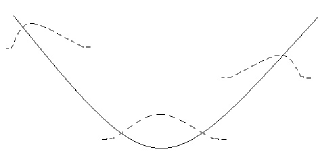
Figure 4: A non-monotone profile. Localized modes in a curved region still have a healthy kinetic term. Modes which can sense the flatness of the well, however, develop the same problems one encounters in the flat Moose case.

The above arguments were mostly qualitative and aimed for an intuitive understanding of the prospects of discretizing AdS space. A more quantitative analysis involving a numerical study of the eigen-modes, their localization and interactions can be found in [13]

7 Conclusions

The ailments of a flat chain is a result of the maximal mixing between the neighboring modes which lead to strong correlations between distant sites. The introduction of a scale difference between the sites acts as a coupling which suppresses the mixing and renders the long wave-length theory healthy. While it is true that the strong coupling scale is lower than expected in the continuum theory (i.e. $M\exp(-ky)$), there is a precise sense in which the effective theory at long distances resembles that of a genuine extra dimension, albeit curved.

Acknowledgments: We thank Nima Arkani-Hamed and Lisa Randall for inspiring this project and providing helpful guidance throughout this work. We gratefully acknowledge Shiyamala Thambyahpillai and Jesse Thaler for helpful discussion.

References

- [1] N. Arkani-Hamed, A. G. Cohen and H. Georgi, Phys. Rev. Lett. 86, 4757 (2001) [arXiv:hep-th/0104005].
- [2] M. Alishahiha, Phys. Lett. B 517, 406 (2001) [arXiv:hep-th/0105153].
- [3] M. Bander, Phys. Rev. D 64, 105021 (2001) [arXiv:hep-th/0107130].
- [4] A. Sugamoto, Prog. Theor. Phys. 107, 793 (2002) [arXiv:hep-th/0104241].
- [5] A. Sugamoto, Grav. Cosmol. 9, 91 (2003) [arXiv:hep-th/0210235].
- [6] N. Kan and K. Shiraishi, Class. Quant. Grav. 20, 4965 (2003) [arXiv:gr-qc/0212113].
- [7] L. Randall, Y. Shadmi and N. Weiner, JHEP 0301, 055 (2003) [arXiv:hep-th/0208120].
- [8] N. Arkani-Hamed, H. Georgi and M. D. Schwartz, Annals Phys. 305, 96 (2003) [arXiv:hep-th/0210184].
- [9] N. Arkani-Hamed and M. D. Schwartz, Phys. Rev. D 69, 104001 (2004) [arXiv:hep-th/0302110].
- [10] M. D. Schwartz, Phys. Rev. D 68, 024029 (2003) [arXiv:hep-th/0303114].
- [11] L. Randall and R. Sundrum, Phys. Rev. Lett. 83, 3370 (1999) [arXiv:hep-ph/9905221].
- [12] A. I. Vainshtein, Phys. Lett. B 39, 393 (1972).
- [13] L. Randall,, M. D. Schwartz, and S. Thambyapillai arXiv:hep-th/0507102.