Observational manifestations of anomaly inflow

Abstract

In theories with chiral couplings, one of the important consistency requirements is that of the cancellation of a gauge anomaly. In particular, this is one of the conditions imposed on the hypercharges in the Standard Model. However, anomaly cancellation condition of the Standard Model looks unnatural from the perspective of a theory with extra dimensions. Indeed, if our world were embedded into an odd-dimensional space, then the full theory would be automatically anomaly free. In this paper we discuss the physical consequences of anomaly non-cancellation for effective 4-dimensional field theory. We demonstrate that in such a theory parallel electric and magnetic fields get modified. In particular, this happens for any particle possessing both electric charge and magnetic moment. This effect, if observed, can serve as a low energy signature of extra dimensions. On the other hand, if such an effect is absent or is very small, then from the point of view of any theory with extra dimensions it is just another fine-tuning and should acquire theoretical explanation.

1 Introduction

In particle physics there is a number of well-established principles (four-dimensional Lorentz invariance, renormalizability, gauge symmetries, etc.), which are believed to underlie a consistent quantum field theory. All these principles are built into the Standard Model (SM) and its great experimental success is a major justification for their validity. However, in continuing search for the consistent description of an emerging physics beyond the Standard Model, one often tries to ease some of these criteria. It is then important to make sure that such modifications do not contradict to the observable data, as well as to find observable signatures of a new model.

Since 1950s [1], one uses the gauge symmetry as a main principle for constructing interactions between elementary particles. It is known, however, that in theories with chiral couplings (i.e. when left and right-handed fermions have different charges with respect to a gauge group), one may encounter a situation when the classically conserved gauge current acquires an anomalous divergence at one loop. It is known that such anomalies destroy consistency of the theory, making it non-unitary [2]. In the Standard Model, where the couplings of fermions are chiral, charges of all particles can be chosen to ensure the absence of all gauge anomalies [7]. It may happen, however, that anomaly-free theory looks like an anomalous one below certain energy scale. An example of such a theory would be an electroweak theory at the energy scale below the mass of top-quark. Then anomaly is canceled by means of Wess-Zumino like terms [8].

Among many possible extensions of the Standard Model there are theories with extra dimensions. Their main idea is that our 4-dimensional physics is embedded into a theory in a higher-dimensional space. The Standard Model fields are then realized as zero modes of a higher-dimensional ones. (An example is given by an approach, often dubbed brane-world models, where zero modes of both matter and gauge fields are localized on the 4-dimensional defect, called brane [9, 10]). Once our 4-dimensional world is just a low-energy sector of a bigger theory, the anomaly analysis changes drastically. For example, if a full theory is anomaly free (say, it is formulated in an odd number of space-time dimensions, where all interactions are vector-like), then one has no reason to expect separate anomaly cancellation for the brane fields (for an explicit example of a brane-world theory with an anomaly on the brane, see [11]). If the theory on the brane is anomalous, then there is a specific type of brane-bulk interaction. It is described by Chern-Simons-like terms in the low-energy effective action in the bulk. These terms are not gauge invariant in the presence of a brane. Therefore, they generate currents, flowing to the brane and thus ensuring the gauge invariance of the full theory. Such mechanism is known for a long time and is often called anomaly inflow [12, 13]. It is quite general and appears in many (physically very distinct) problems: in quantum Hall effect [14, 15], in various field theories with solitonic objects in them (see e.g. [17, 18, 19]), in string and M-theory [20, 21, 22, 23]. Thus, in the brane-world models a number of questions arises:

1. Can one distinguish between a purely 4-dimensional anomaly-free theory, and a theory (also anomaly-free!) in which anomaly is canceled by a small inflow from extra dimensions? What new observable effects appear in the latter situation?

2. Is it possible to discriminate at low-energies between two different completions of anomalous 4-dimensional effective theory: the one, where anomaly is canceled by inflow from higher dimensions and purely 4-dimensional one, where at higher energies there exist additional particles, which ensure anomaly cancellation (c.f. [8]).

3. For generic values of hypercharges the minimal Standard Model is anomalous. However, for any hypercharges, electrodynamics is still vector-like. Can this anomaly nevertheless be observed if this anomalous theory is embedded into a consistent higher-dimensional one?

4. What are experimental constraints for the parameters describing anomaly mismatch? Can the above observations serve as tests in the search for extra dimensions?

In this paper we will attempt to answer the questions 1–3. The question 4 will be addressed in our next paper [24]. We would like to note also that in this paper (as well as in the subsequent paper [24]) we study only gauge anomalies. The global chiral anomalies in brane-worlds and corresponding complicated vacuum structure of gauge fields has been discussed in [25].

We consider a theory on a brane, which is anomalous, while the bulk effective action possesses a Chern-Simons-like term, responsible for an inflow current. A naive answer to the question (1) then would seem to be the following: as anomaly means gauge current non-conservation, one could expect that particles escape from the brane to extra dimensions. This would look like a loss of unitarity from a purely 4-dimensional point of view, however higher-dimensional unitarity would still be preserved. Anomalous current then is simply a flow of such zero-mode particles into the bulk. However, this answer is incorrect. Indeed, phenomenologically acceptable brane-world scenario must have a mass gap between zero modes and those in the bulk for both fermions and non-Abelian gauge fields [26, 27]. Alternatively, the rate of escape of the matter from a brane must be suppressed in some way (see e.g. [28]). As a result, the low-energy processes on the brane simply cannot create an excitation, propagating in the bulk. If no matter can escape the brane (or flow onto it) – what is then an inflow current, which should be non-zero even for weak fields causing anomaly in four-dimensional theory? One seems to be presented with a paradox.

We show that in reality the inflow current by its nature is a vacuum or non-dissipative current. What we mean by that is the following. Usually in electrodynamics one needs to create particles from a vacuum to generate an electric current. Such a process is only possible if the available energy is larger than the mass of the particles in the bulk. Therefore, weak electric fields on the brane cannot induce a current, carried by the bulk modes. However, anomaly inflow current is different. First, it is perpendicular to the field, does not perform a work and thus is not suppressed by the mass of a particle in the bulk. Second, such a current is not carried by any real particles excited from the vacuum, being rather a collective effect, resulting from a rearrangement of the Dirac sea. This simple observation is in fact very important. Essentially, it means that anomaly inflow is a very special type of brane-bulk interaction.

Namely, we show that in the presence of parallel magnetic and electric fields the latter changes as if photon had acquired mass. As a result the spatial distribution of an electric field changes, in particular it appears outside the plates of the capacitor. Similarly, an electric field of an point-like electric charge changes from Coulomb to Yukawa, when the charge is placed in a magnetic field. The dynamics of the screening of electric charge happens to be quite peculiar and can be shown to lead to the temporary appearance of dipole moment of elementary particles.

At first, we conduct our analysis in $U(1)$ gauge theory with the chiral couplings to a matter. One example of such a theory would be an electrodynamics, where left and right-handed particles have different electric charges. The masses of such particles can then be generated only via the Higgs mechanism with a charged Higgs field, which means that a photon in such a theory becomes massive. A different example is a theory, where axial current comes from a neutrino with a small electric charge. In such theory photon would remain massless.

Then we analyze the version of the Standard Model where electric charges of electron and proton differ. We show that although low-energy electrodynamics in this theory is vector-like, there exist effects, similar to those, described above.

We would like to stress again that in the theories with extra dimensions there is no immediate reason to expect that four-dimensional anomaly is so small as it follows already from present experimental constraints on the corresponding parameters. The effects which would follow from the existence of an anomaly inflow are observable, but quite peculiar. They do not change drastically physical content of the theory and can be ruled out or constrained only experimentally. Thus in those brane-world scenarios, in which higher-dimensional theory is automatically anomaly free, we are facing yet another fine-tuning puzzle.

For distinctness we will often refer to a simple brane-world: the fermions in the background of a kink, realizing a 4-dimensional brane, embedded into a 5-dimensional space as in [9] (although main effects are believed to be model-independent). We localize gauge fields in a spirit of [30, 28, 31, 32], introducing an exponential warp-factor. Such warp-factor can arise dynamically because of the fermionic zero modes [33]. Zero modes of both types of fields are separated by mass gaps from the corresponding bulk modes.

The paper is organized as follows. We begin section 2 with describing a model of chiral electrodynamics, embedded into a 5-dimensional $U(1)$ theory and analyze the microscopic structure of the inflow and details of anomaly cancellation. Next, we turn in Section 3 to the question of possible extensions of the Standard Model, such that it would admit an anomaly. We consider one-parameter family of such modifications, with the free parameter being the difference of (absolute values of) electric charges of proton and electron. In such model particles also acquire an anomalous dipole moment. We discuss it in the Section 3.3. We conclude with a discussion of future extensions of this work and some speculations.

Finally, we would like to stress that in this paper we conducted analysis on the level of classical equations of motion. We discuss some aspects of quantum theory and the validity of our approach in 4.

2 Anomalous electrodynamics and its observational
signatures.

2.1 5-dimensional electrodynamics in the background of a kink

We start our analysis considering in this section the simplest model which nevertheless catches main effects we are interested in. Namely, we will discuss a four-dimensional $U(1)$ theory with anomalous chiral couplings to the fermions. Such a theory suffers from a gauge anomaly, meaning that on the quantum level its unitarity is lost [3, 2, 7, 4]. Thus it cannot describe physics of a 4-dimensional world. However, if one thinks about such an anomalous theory as living on a brane, embedded in a 5-dimensional theory, situation changes. Five-dimensional theory is anomaly-free (all couplings there are vector-like) and therefore there should exist a special type of interaction (anomaly inflow [12, 13]) between the theories on the brane and in the bulk, which ensures the unitarity and consistency of the total system. Below we demonstrate this mechanism in details.

For definiteness we will illustrate our steps by using a concrete model of localization of both fermions and gauge fields. Consider the following theory:

$$S=-\frac{1}{4\,\mathbf{e}^{2}}\int d^{5}x\,\Delta(x^{4})F_{ab}^{2}+\int d^{5}x\,\sum_{f=1}^{2}\bar{\Psi}_{f}(x)\Bigl{(}i{\mathop{\hbox to0.0pt{$\displaystyle D$\hss}{\,\mbox{\large/}}}\nolimits}_{f}+m_{f}(x^{4})\Bigr{)}\Psi_{f}(x)\>.$$ (2.1)

Here $\,\mathbf{e}$ is a five-dimensional charge, with the dimensionality of $(\mathrm{length})^{\frac{1}{2}}$. There are two fermions $\Psi_{1,2}$, interacting with the gauge fields with the different charges: ${\mathop{\hbox to0.0pt{$\displaystyle D$\hss}{\,\mbox{\large/}}}\nolimits}_{f}=\mathop{\hbox to0.0pt{$\displaystyle\partial$\hss}{\mbox{\large/}}}+\frac{\,\mathbf{e}_{f}}{\,\mathbf{e}}\mathop{\hbox to0.0pt{$\displaystyle A$\hss}{\,\mbox{\large/}}},\,\,\mathbf{e}_{1}\neq\,\mathbf{e}_{2}$. The fermionic mass terms $m_{1}(x^{4})=-m_{2}(x^{4})$ have a “kink-like” structure in the direction $x^{4}$, realizing the brane: $m_{1}(x^{4}\to\pm\infty)\to\pm m_{\psi}$. As it is well-known (see e.g. [9]), in this model one has chiral fermion zero modes localized on the brane and a continuous spectrum in the bulk, separated from the zero mode by the mass gap $m_{\psi}$. Localization of the zero mode of gauge field is achieved by introduction of a warp-factor $\Delta(x^{4})$. Whenever $\int dx^{4}\Delta(x^{4})$ is convergent the system has a zero mode with the constant profile in the 5th direction. Warp-factor $\Delta(x^{4})$ looks like an $x^{4}$ dependent coupling constant in the action (2.1), getting infinite as $|x^{4}|\to\infty$. The lattice study of [32] has confirmed that the perturbative and non-perturbative analysis of (2.1) give the same result for the zero mode up to the energies of the order of the mass gap, at least for $2+1\to 1+1$ reduction. We will assume that this is the case for $4+1\to 3+1$. Depending on the warp-factor, the spectrum of gauge field may be discrete or continuous with or without the mass gap between the zero and bulk modes [30, 28, 31]. We will often use $\Delta(x^{4})=e^{-2M\left|x^{4}\right|}$ in which case the zero mode is separated from the bulk continuum by the mass gap $M$ [31]. The nature of the warp-factor $\Delta(x^{4})$ is not essential here, it can originate from that of the metric or can arise dynamically, coming from fermionic zero modes [33].

A low-energy effective action for the gauge fields of the theory (2.1) will contain terms, describing interaction between the brane and the bulk:

$$S_{\text{5d}}=-\frac{1}{4\,\mathbf{e}^{2}}\int d^{5}x\,\Delta(x^{4})\,F^{2}_{ab}+S_{{\textsc{cs}}}+S_{{\mathrm{z.m}}}\,.$$ (2.2)

The origin of two last terms is the following. The computation of the fermionic path integral of our theory is separated into the determinant of the 5-dimensional bulk modes of the fermions and that of the 4-dimensional chiral fermionic zero modes. In the former case one can show (essentially repeating the computations of [34]), that after integrating out the non-zero modes of the fermions, the 5-dimensional effective action of the model (2.1) acquires an additional contribution of Chern-Simons type

$$S_{\textsc{cs}}=\frac{1}{4}\int dx^{5}\,\kappa(x^{4})\epsilon^{abcde}A_{a}F_{bc}F_{de}\,.$$ (2.3)

Compared to the usual case [34, 35], Chern-Simons term in models like (2.1) acquires additional factor $\kappa(x^{4})$. It is proportional to the difference of the charges of the five-dimensional fermions and depends on the profile of the domain wall. In the limit of an infinitely thin wall and the large fermionic mass gap $\kappa(x^{4})=\kappa_{0}\mathop{\mathrm{missing}}{sign}(x^{4})$. Below we sketch the derivation of this function.

Terms like (2.3) generically appear in the theories with anomaly inflow [13, 17, 21, 22, 23, 18, 19]. In situations with more than one extra dimension an effective action will have similar structure, with the fifth coordinate being suitably chosen radial coordinate. Such terms can also appear for non-Abelian fields.

Evaluating of the determinant of the 4-dimensional Dirac operator in the background of the gauge field (and, possibly, Higgs field, see below), we get $S_{\mathrm{z.m}}$. Let us denote the 4-dimensional charges of the left and right-handed fermionic zero modes as $e_{L}/e$ and $e_{R}/e$. They are proportional to their 5-dimensional counterparts $\,\mathbf{e}_{1}$ and $\,\mathbf{e}_{2}$ and thus $e_{L}\neq e_{R}$. As a result $S_{\mathrm{z.m}}$ is not gauge invariant. The manifestation of this fact is the anomalous divergence of the gauge current at one-loop level:

$$\partial_{\mu}\langle j^{\mu}_{\mathrm{z.m}}\rangle=\frac{e_{R}^{3}-e_{L}^{3}}{16\pi^{2}e^{3}}\epsilon^{\mu\nu\lambda\rho}F_{\mu\nu}F_{\lambda\rho}\,\delta(x^{4})\,,\qquad\text{where}\quad\langle j^{\mu}_{\mathrm{z.m}}\rangle\equiv\frac{\delta S_{\mathrm{z.m}}}{\delta A_{\mu}}\>.$$ (2.4)

The action (2.3) is also non-gauge invariant, and the variations of these two terms cancel each other (as we will demonstrate below). Divergence of the current (2.4) is proportional to the transversal profile of the fermion zero modes. In this paper we will be interested in the characteristic energy scales much less than the mass gap of the gauge fields $M$, which is in turn much less than the fermionic mass gap: $M\ll m_{\psi}$. Therefore the profile of the fermion zero mode can be approximated by the delta-function $\delta(x^{4})\approx 2m_{\psi}e^{-m_{\psi}|x^{4}|}$, which appears in eq. (2.4).

Equations of motion coming from the action (2.2) are:

$$\frac{1}{\,\mathbf{e}^{2}}\partial_{b}\Bigl{(}\Delta(x^{4})F^{\mu b}\Bigr{)}=J^{\mu}_{\textsc{cs}}+\langle j_{\mathrm{z.m}}^{\mu}\rangle,\qquad a,b=0,\dots,4$$ (2.5)

and

$$\frac{1}{\,\mathbf{e}^{2}}\Delta(x^{4})\partial_{\mu}F^{4\mu}=J^{4}_{\textsc{cs}},\qquad\mu=0,\dots,3.$$ (2.6)

In the right hand side of eq. (2.5) there is a current of the zero modes $j_{\mathrm{z.m}}^{\mu}$ (we will omit brackets $\langle\dots\rangle$ from now on). The variation of the effective action $S_{\mathrm{z.m}}$ with respect to the $A_{4}$ is equal to zero.

The current $J_{\textsc{cs}}$ in the right hand side of eqs. (2.5)–(2.6) is defined via

$$J^{a}_{\textsc{cs}}(x^{a})=\frac{\delta S_{\textsc{cs}}}{\delta A_{a}}=\frac{3}{4}\kappa(x^{4})\epsilon^{abcde}F_{bc}(x^{a})F_{de}(x^{a})+\frac{1}{2}\kappa^{\prime}(x^{4})\delta^{a}_{\mu}\epsilon^{\mu\nu\lambda\rho}A_{\nu}F_{\lambda\rho},\quad\kappa^{\prime}(x^{4})=\frac{d\kappa(x^{4})}{dx^{4}}\>.$$ (2.7)

Note that in the right hand side of eq. (2.7) there is a term, proportional to the derivative of $\kappa(x^{4})$. This term is non-zero only in the vicinity of the brane (as $\kappa^{\prime}(x^{4})$ is proportional to the delta-function of $x^{4}$). Thus, essentially it corresponds to the modification of definition of the brane current $j^{\mu}_{\mathrm{z.m}}$ (2.4). This additional term is responsible for making anomaly of the zero modes gauge invariant [17, 18], as the inflow current (2.4) is always gauge invariant in the $U(1)$ case. Thus, terms proportional to $\kappa^{\prime}(x^{4})$ correspond to the local counterterms, shifting between the covariant and consistent anomalies [36]. In what follows we will always consider covariant anomaly of the brane modes and ignore terms in the bulk, proportional to the $\kappa^{\prime}(x^{4})$. The Chern-Simons current $J^{a}_{\textsc{cs}}$ is a non-dissipative one as it does not perform a work due to its antisymmetric structure. In addition to that it does not depend on the mass of the fermions in the bulk and hence is not suppressed by the mass gap. If a gauge field has four-dimensional components with $\epsilon^{\mu\nu\lambda\rho}F_{\mu\nu}F_{\lambda\rho}\neq 0$, there exists a current $J^{4}_{\textsc{cs}}$, flowing onto the brane from the extra dimension [13].

Trivial consequence of eqs. (2.5)–(2.6) is

$$\partial_{a}J_{\textsc{cs}}^{a}+\partial_{\mu}j_{\mathrm{z.m}}^{\mu}=\frac{1}{\,\mathbf{e}^{2}}\partial_{a}\partial_{b}F^{ab}=0\>.$$ (2.8)

It means that if coefficients in front of the $S_{\textsc{cs}}$ and $S_{\mathrm{z.m}}$ were not correlated, by virtue of (2.4) the solutions of eq. (2.8) would be field configurations with $\epsilon^{\mu\nu\lambda\rho}F_{\mu\nu}F_{\lambda\rho}=0$. However, to preserve the gauge-invariance in the action (2.2) the divergences of currents in the left hand side of (2.8) should be equal. From the definition (2.7) one can see that

$$\partial_{a}J^{a}=\frac{3}{4}\kappa^{\prime}(x^{4})\epsilon^{\mu\nu\lambda\rho}F_{\mu\nu}F_{\lambda\rho}=\frac{3}{2}\kappa_{0}\epsilon^{\mu\nu\lambda\rho}F_{\mu\nu}F_{\lambda\rho}\delta(x^{4})\>.$$ (2.9)

Comparing (2.9) with eq. (2.4) we can choose the coefficient of $\kappa_{0}$ of the function $\kappa(x^{4})$ so that the current $J_{\textsc{cs}}$ cancels the anomalous divergence of the current $j_{\mathrm{z.m}}^{\mu}$ and make the theory (2.2) consistent and gauge-invariant. Namely

$$\kappa(x^{4})=\kappa_{0}\mathop{\mathrm{missing}}{sign}(x^{4}),\quad\text{where}\quad\kappa_{0}\equiv\frac{e_{L}^{3}-e_{R}^{3}}{24\pi^{2}e^{3}}\>.$$ (2.10)

Microscopical calculations of $\kappa(x^{4})$ confirm that this is indeed the case.

The relation between 5-dimensional fields $F_{\mu\nu}$, entering eqs. (2.5)–(2.6) and the 4-dimensional ones is given by:

$$\frac{1}{e^{2}}\text{{F}}_{\mu\nu}=\frac{1}{\,\mathbf{e}^{2}}\int^{\infty}_{-\infty}dx^{4}\Delta(x^{4})F_{\mu\nu}\>.$$ (2.11)

Here $e$ is a four-dimensional $U(1)$ coupling constant, related to the 5-dimensional one via

$$\frac{1}{e^{2}}=\frac{1}{\,\mathbf{e}^{2}}\,\int dx^{4}\Delta(x^{4})$$ (2.12)

(to see that, one should substitute $F_{\mu\nu}$, independent on the 5th coordinate, into the kinetic term in (2.2) and integrate over $x^{4}$). Field $\text{{F}}_{\mu\nu}$ satisfies the 4-dimensional Maxwell equations $\partial_{\nu}\text{{F}}^{\mu\nu}=e^{2}\text{{j}}^{\mu}$ with the current in the right hand side given by:

$$\text{{j}}^{\mu}=\int^{\infty}_{-\infty}dx^{4}\,\left(j^{\mu}_{\mathrm{z.m}}+J^{\mu}_{\textsc{cs}}-\partial_{4}\Bigl{(}\Delta(x^{4})F^{\mu 4}\Bigr{)}\right)\>.$$ (2.13)

This current is conserved: $\partial_{\mu}\,\text{{j}}^{\mu}=0$ as a consequence of eqs. (2.6) and (2.8).

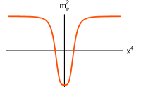
Figure 1: Profile of the mass of the Higgs field.

In the theory (2.1) fermionic zero modes on the brane are massless. To make this model more realistic, we should add mass to these zero modes as well. The only way to make the electro-dynamics anomalous is to take left and right moving fermions with different electric charges. Thus one can only introduce a mass term via the Higgs mechanism with an electrically charged Higgs field, i.e. to add the following term to the bulk Lagrangian (2.1):

$$S_{\phi}=\int d^{5}x\left[\bigl{|}D_{a}\phi\bigr{|}^{2}-m_{\phi}^{2}(x^{4})|\phi|^{2}-\frac{\lambda}{4}|\phi|^{4}+f\bar{\Psi}_{1}\Psi_{2}\phi+\mathrm{h.c.}\right]\>,$$ (2.14)

where $D_{\mu}\phi=i\partial_{\mu}\phi+(\frac{e_{L}}{e}-\frac{e_{R}}{e})A_{\mu}\phi$ and the Higgs mass $m_{\phi}^{2}(x^{4})$ is negative at $x^{4}=0$ and tends to the positive constant in the bulk, as $|x^{4}|\to\infty$ (Figure 1). Thus Higgs field has a non-trivial profile $\phi(x^{4})$, with $\phi(0)\neq 0$ and $\phi(x^{4})\to 0$ at $x^{4}\to\pm\infty$. So the symmetry is restored far from the domain wall. The Higgs mass far from the brane is taken to be large, so that the scalar is localized on a brane. The Higgs field has an expectation value, which on the brane is $\langle\phi(0)\rangle\sim v$ (we take the scalar’s self-coupling $\lambda$ to be large, so that Higgs mass $m_{H}$ is much bigger than $fv$ – Yukawa mass of the fermions on the brane). As the Higgs field is charged, the photon should acquire mass for $x^{4}\approx 0$). To determine it exactly one needs to find the spectrum of the theory with action given by the sum of (2.1) and (2.14), but for us it is only important that $m^{2}_{\gamma}\sim\kappa_{0}^{2}$, where parameter $\kappa_{0}$ was defined in (2.10). In Section 3 we will analyze the consequences of anomaly inflow in the Standard Model, where Yukawa mass of the fermions does not necessarily lead to the massive photon.

Dynamics of the Higgs field $\phi$ simplifies in the limit of the large (compared to the energy scale of the processes on the brane) VEV $v$. In this limit it is convenient to work in the unitary gauge, in which the phase of the Higgs field is fixed (e.g. via $\phi=|\phi|$). In the regions of space where the gauge field has non-trivial $F_{\mu\nu}$, it is impossible to have $|\phi|=\mathrm{const}$ [37]. However, variations of the $|\phi(x^{a})|-v$ are suppressed by the Higgs’s VEV, we can neglect them and take $\phi=v=\mathrm{const}$ on the brane. Now the vector field is massive and longitudinal component becomes a physical degree of freedom. From equations of motion one can obtain the following condition on the field $A_{a}(x^{a})$:

$$\partial_{a}\bigl{(}m^{2}_{\gamma}(x^{4})A^{a}\bigr{)}+\partial_{\mu}j^{\mu}_{\mathrm{z.m}}+\partial_{a}J^{a}_{\textsc{cs}}=0\>.$$ (2.15)

Eq. (2.15) is just an expression of the gauge invariance of the total action. Divergences of $j_{\mathrm{z.m}}$ and $J_{\textsc{cs}}$ precisely cancel each other (2.8). Therefore eq. (2.15) implies that

$$\partial_{a}\bigl{(}m^{2}_{\gamma}(x^{4})A^{a}\bigr{)}=0\>.$$ (2.16)

Once we have added the mass to the zero mode fermions, we can integrate them out and obtain effective action $S_{\mathrm{z.m}}$ (2.2), written in unitary gauge. The variation of this action with respect to $A_{\mu}$ gives gauge invariant current [8]:

$$j^{\mu}_{{\mathrm{z.m}}}=3\kappa_{0}\epsilon^{\mu\nu\lambda\rho}\frac{\phi^{*}\overleftrightarrow{D}_{\nu}\phi}{v^{2}}F_{\lambda\rho}\delta(x^{4})\>.$$ (2.17)

We will often call this current the D’Hoker-Farhi current denote it $j^{\mu}_{\textsc{df}}$. In the unitary gauge eq. (2.17) becomes

$$j^{\mu}_{{\textsc{df}}}=3\kappa_{0}\epsilon^{\mu\nu\lambda\rho}A_{\nu}F_{\lambda\rho}\delta(x^{4})\>.$$ (2.18)

This current has a divergence, equal to that of the Chern-Simons current ($\partial_{\mu}j^{\mu}_{\textsc{df}}=-\partial_{a}J^{a}_{\textsc{cs}}$):

$$\partial_{\mu}j^{\mu}_{\textsc{df}}=\frac{3}{2}\kappa_{0}\epsilon^{\mu\nu\lambda\rho}F_{\mu\nu}(x^{\mu},x^{4})F_{\lambda\rho}(x^{\mu},x^{4})\delta(x^{4})\>.$$ (2.19)

A purpose of this work is to explore in details this anomaly cancellation mechanism. Namely, what constitutes the inflow? Zero modes of fermions are confined to the brane and cannot propagate in the bulk, while bulk modes are massive and cannot be excited at low energies. Another question is whether 4-dimensional observer can distinguish between an anomaly-free, intrinsically 4-dimensional theory and 5-dimensional (anomaly-free!) brane-world theory, in which a very small anomaly of the 4-dimensional fermions on the brane is canceled by an inflow from the bulk.

2.2 Anomalous electric field of a capacitor

As we have seen, on the microscopic level anomaly inflow is a collective effect of reorganization of the Dirac see of the massive fermions in the bulk in the presence of a field configuration with non-zero $\epsilon^{\mu\nu\lambda\rho}F_{\mu\nu}(x^{a})F_{\lambda\rho}(x^{a})|_{x^{4}=0}\sim(\vec{E}\cdot\vec{H})$.

The simplest way to obtain non-zero $\vec{E}\cdot\vec{H}$ is to choose both $E$ and $H$ to be parallel to each other and constant (in $x^{\mu}$) in some region on the brane. We realize such fields by two parallel infinite plates in the vacuum, separated in the direction $x^{1}$ by the distance $2d$ – a capacitor with initial charge densities $\pm\sigma_{0}$ on plates, placed in the magnetic field. Magnetic field is created by an (infinite in the $x$-direction) solenoid with the radius $R$.

Before these fields are turned on, the vacuum structure on the classical level is unchanged and there is no difference with non-anomalous theory. Also, the effects of anomaly are controlled by the parameter $\kappa_{0}$, which is naturally assumed to be very small. That is why the most natural setup to study the anomaly inflow is qualitatively the following. We assume that the vacuum current is zero and an electric field is equal to its value for non-anomalous theory. Then we turn on a parallel magnetic field and expect that small (perturbative in $\kappa_{0}$) inflow currents start to change the charge distribution on the brane trying to compensate the anomalous field configuration. According to this picture, in Section 2.2.1 we will choose initial condition describing the absence of anomalous vacuum structure and will consider an initial stage of inflow (linear in time) perturbatively, in the first order in $\kappa_{0}$.

We will see, however, that this naive approach does not work and perturbation theory breaks down. Therefore, we will have to study the full non-linear equations non-perturbatively in $\kappa_{0}$. Then, as we will show in Section 2.2.2, a non-analytic in $\kappa_{0}$ static solution exists. The properties of this solution will define the main observable effect of the anomaly inflow, studied in the present paper. It is, nevertheless, instructive to study the dynamical problem to understand qualitatively how this state is formed. As we will see in Section 2.2.3, from the 4-dimensional point of view the picture of the inflow given by perturbation theory is qualitatively correct and knowing the non-perturbative static solution one can define it properly.

2.2.1 Linear stage of anomaly inflow: naive perturbative treatment

As in general we expect the parameter $\kappa_{0}$ to be extremely small, we will try to solve the Maxwell equations (2.5)–(2.6) by perturbation theory in $\kappa_{0}$. To find linear in time corrections to the fields at $t=0$, we should specify the initial values of all fields. Our initial conditions should satisfy the Gauss constraint

$$\frac{1}{\,\mathbf{e}^{2}}\Bigl{(}\partial_{z}\bigl{(}\Delta(z)E^{z}\bigr{)}+\Delta(z)\mathop{\mathrm{div}}\vec{E}\Bigr{)}=J^{0}_{\textsc{cs}}+j_{\textsc{df}}^{0}+\sigma_{0}\delta(z)\Bigl{(}\delta(x+d)-\delta(x-d)\Bigr{)}\>,$$ (2.20)

where $J^{0}_{\textsc{cs}}$ and $j^{0}_{\textsc{df}}$ are expressed in terms of components $F_{ab}$ and are both proportional to the $\kappa_{0}$ (c.f. (2.7) and (2.18) correspondingly). Because we have added a charged Higgs field (2.14) and the electrodynamics became massive, specifying initial values of $F_{ab}$ is not enough and one should also set values of the gauge potential at $t=0$. We choose all but $A_{\theta}$ components $A_{a}$ initially equal to zero (see Appendix A for details). The time derivatives of $A_{a}$ can then be extracted knowing electric fields at $t=0$ and using condition (2.16). In this paper we restrict our analysis only to such initial conditions. In general initial conditions on the vector field $A_{a}$ will depend on how one turns on electric and magnetic fields. Corresponding analysis (similar to that of [38]) will be presented elsewhere.

In addition to these initial condition we will choose as a zeroth approximation such configuration of electromagnetic fields $F_{ab}$ that $J^{0}_{\textsc{cs}}\bigr{|}_{t=0}=0$. The reason for that is as follows: from (2.7) one has $J^{0}_{\textsc{cs}}=\frac{3}{4}\kappa(z)F_{xz}H^{x}$. In the absence of anomaly $F_{xz}$ would be equal to zero for our configuration of charges. Therefore, it is natural to assume that initially $F_{xz}$ is equal to zero in the full theory as well. Initial conditions $J^{0}_{\textsc{cs}}=0$ and $j^{0}_{\textsc{df}}=0$ mean that we should prepare an electric field configuration, satisfying 5-dimensional Gauss constraint in the theory with $\kappa_{0}=0$ (we will mark these fields by the symbol ⁽⁰⁾). Then we find (perturbative) corrections to these fields due to anomalous current and analyze effects arising on the initial (linear) stage of inflow. The details of the computations can be found in Appendix A.1, here we only quote the main results.

With our choices for the fields $F_{ab}^{(0)}$, initially only time component of the D’Hoker-Farhi current changes with time (see Appendix A.1):

$$\partial_{t}j^{0}_{\textsc{df}}(x^{\mu})\biggr{|}_{t=0}\hskip-4.30554pt=-6\kappa_{0}E_{x}^{(0)}(x,z)H_{x}^{(0)}(r,z)\delta(z)\>,$$ (2.21)

If the theory were purely four-dimensional, eq. (2.21) would have described the rate of anomalous particle production, essentially the measure of non-unitarity of the theory. In the 5-dimensional brane-world the interpretation of eq. (2.21) is quite different. Namely, one should not think about the inflow current, as “bringing particles to the brane”. This is obvious as all the light (zero mass) particles are confined to the brane and do not propagate in the bulk, while the fermions, which live in the bulk are too massive to be excited at low energies. Thus, inflow current (2.7) is essentially a vacuum current – redistribution of the particle density without actual creation of the charge carriers. This fact can be checked by the direct microscopic computations of the vacuum average of $\left\langle{0}\right|J_{\textsc{cs}}^{z}\left|{0}\right\rangle$ in the full theory (2.1). The divergence $\partial_{a}J_{\textsc{cs}}^{a}$ is non-zero only in the position of the brane $z=0$ and thus modifies the charge density only there (which is reflected by the delta-function in eq. (2.21)). One may think of the effect of the vacuum current as of a dielectric susceptibility of the vacuum of four-dimensional theory, embedded in the 5-dimensional space-time.

Notice, that since there is no $J^{0}_{\textsc{cs}}$, eq. (2.21) means that the total electric charge density changes with time. If the charge density changes in the finite volume on the brane, this leads to the change of both $E^{x}$ and $E^{z}$. (If initial field $E^{x}$ and $H^{x}$ uniformly filled all the brane and were localized in $z$ direction, then the appearance of the anomalous density would not lead to the change of the $x$ component of the electric field. The change in $E^{z}$ would be unobservable, since this field is antisymmetric in $z$ and so $\int dz\,\Delta(z)E^{z}=0$). For the case when $\vec{E}\cdot\vec{H}$ is non-zero only in the finite volume on the brane we explicitly find the change in $E^{x}$ by solving Maxwell equations (2.5)–(2.6):

$$E_{x}^{(1)}(x^{a})=-6\,\mathbf{e}^{2}\frac{\kappa(z)}{\Delta(z)}E_{z}^{(0)}(x,z)H^{(0)}_{x}(r,z)t+{\cal O}(t^{2})\>.$$ (2.22)

Now one can see that our perturbation theory approach has a problem. Indeed, although $E_{x}^{(1)}$ is proportional to $\kappa_{0}$, it grows in $z$ as $\frac{1}{\Delta(z)}$ while $E_{x}^{(0)}$ decays as $|z|\to\infty$. The correction term (2.22) becomes larger than $E_{x}^{(0)}$ at $|z|\sim-\frac{\log\kappa_{0}}{M}$. Eq. (2.22) gives correction to the 5-dimensional electric field. The corresponding 4-dimensional field is obtained via (2.11). As shown in Appendix A.1, the integral in (2.11) is saturated at $|z|\sim Mx^{2}$ where characteristic $|x|\gg\frac{1}{M}$. Therefore in the physically relevant region

$$E_{x}^{(1)}>E_{x}^{(0)}\quad\text{for}\quad|z|\gtrsim-\frac{\log\kappa_{0}}{M}\>.$$ (2.23)

Thus, we see that the naive form of perturbation theory does not work. It means that something was wrong with our qualitative picture of the inflow and that we have to study full equations non-perturbatively.

2.2.2 Analysis of a static solution

We have seen in the previous section that effects, caused by anomaly inflow are non-perturbative. As the full system of non-linear Maxwell equations is too complicated to solve exactly, we will compute a static solution. This means that we do not study how anomaly inflow modifies the initial fields, but rather describe a final state of the inflow. We will consider the simplest case: a capacitor with infinite plates, when these equations are reduced to the $2+1$ ones. Below we will only sketch the computations, for details reader should refer to Appendix B. We will return to the perturbation theory in the Section 2.2.3.

For static solution we can describe the electric field in terms of the electro-static potential $\Phi$: $E_{i}=-\partial_{i}\Phi$, $E_{z}=-\partial_{z}\Phi$. Then the Gauss constraint can be re-written as (see Appendix B for details):

$$\partial_{z}\Bigl{(}\Delta(z)\partial_{z}\Phi\Bigr{)}+\Delta(z)\nabla^{2}\Phi=\frac{36\,\mathbf{e}^{4}\kappa_{0}^{2}}{r^{2}\Delta(z)}\Bigl{(}F_{r\theta}^{2}+F_{x\theta}^{2}+F_{\theta z}^{2}\Bigr{)}\Phi+\,\mathbf{e}^{2}q(x)\delta(z)+j^{0}_{\textsc{df}}\>,$$ (2.24)

where $\nabla^{2}$ is a 3-dimensional Laplacian in the coordinates $x,r,\theta$. Components $F_{r\theta},\,F_{x\theta}\,F_{z\theta}$ can all be expressed via single function $A_{\theta}$ (because we choose all the gauge connection to be $\theta$ independent). The Maxwell equation (2.5) for $\mu=\theta$ becomes then an equation for $A_{\theta}$:

$$\partial_{z}\Bigl{(}\Delta(z)\partial_{z}A_{\theta}\Bigr{)}+\Delta(z)\nabla^{2}A_{\theta}=\frac{36\,\mathbf{e}^{4}\kappa_{0}^{2}\Phi}{r^{2}\Delta(z)}\Bigl{(}\partial_{x}A_{\theta}\,\partial_{x}\Phi+\partial_{z}A_{\theta}\partial_{z}\Phi+\partial_{r}A_{\theta}\partial_{r}\Phi\Bigr{)}\>.$$ (2.25)

We will analyze this solution as follows. First, we notice that if the right hand side of eq. (2.25) were identically zero, then there would be a solution $F_{r\theta}=rH^{x}$, $H^{x}=\mathrm{const}\equiv\text{{H}}_{0}$, $F_{x\theta}=F_{\theta z}=0$. Then one can easily find an explicit solution of eq. (2.24) (under these assumptions Gauss law becomes identical to that of the $2+1$ dimensional case with the point-particle as the source). After that we show that corrections to the found solutions of eqs. (2.24)–(2.25) due to the non-zero right hand side of (2.25) are of the order $\kappa_{0}^{2}$. Note, that potentially the first terms in the right hand sides of both (2.24) and (2.25) can be non-perturbative, as they are proportional to the $\frac{1}{\Delta(z)}$. This is precisely why the naive perturbation theory of the Section 2.2.1 did not work.

After the Fourier transform in $x,r,\theta$-directions: ($\nabla\to i\vec{p}$) and a substitution $\Phi=\frac{\psi_{p}(z)}{\sqrt{\Delta(z)}}$ equation (2.24) becomes

$$(\hat{H}+p^{2})\psi_{p}(z)=-\,\mathbf{e}^{2}q_{0}\delta(z)\>,$$ (2.26)

where operator $\hat{H}$ does not depend on $p$:

$$\hat{H}=-\partial_{z}^{2}+\Bigl{(}36\,\mathbf{e}^{4}\kappa_{0}^{2}\text{{H}}_{0}^{2}\,e^{4M|z|}+M^{2}-2M\delta(z)\Bigr{)}\>.$$ (2.27)

Let us denote the eigen-function of (2.27) by $\psi_{n}(z)$ and its eigen-values by $m_{n}^{2}$: $\hat{H}\psi_{n}(z)=m_{n}^{2}\psi_{n}(z)$. One can show (see Appendix B) that

$$m_{0}^{2}=12\kappa_{0}\,\mathbf{e}^{2}\text{{H}}_{0}M+{\cal O}(\kappa_{0}^{2}\log\kappa_{0})\approx 12\kappa_{0}e^{2}\text{{H}}_{0}\quad\text{and}\quad m_{n}^{2}>M^{2}\quad\text{for}\quad n>0$$ (2.28)

(recall that $e^{2}$ is a four-dimensional coupling constant (2.12)). Notice that $m_{0}$ depends only on the four-dimensional quantities (electro-magnetic coupling constant $e^{2}$ and the magnetic field $\text{{H}}_{0}$ measured by a 4-dimensional observer)! The eigen-function for the eigen-value $m_{0}^{2}$ is given by

$$\psi_{0}(z)=\frac{m_{0}}{\sqrt{2\pi M}}K_{\nu}\left(\tfrac{m_{0}^{2}}{4M^{2}}\,e^{2M|z|}\right)\quad\text{where}\quad\nu=\frac{1}{2}\sqrt{1-\frac{m_{0}^{2}}{M^{2}}}.$$ (2.29)

Here $K_{\nu}(u)$ is a modified Bessel function of the second kind and $c_{0}$ is a normalization constant. The solution of eq. (2.24) can be easily found for any charge distribution $q(x)$. For the point-particle in the uniform magnetic field an electrostatic potential, created by the particle will be of the Yukawa form:

$$\Phi(x,r,z)=\frac{q_{0}}{4\pi}\frac{e^{-m_{0}\sqrt{x^{2}+r^{2}}}}{\sqrt{x^{2}+r^{2}}}\chi_{0}(z)\>,$$ (2.30)

where the mass $m_{0}$ depends on the anomaly coefficient and the magnetic field $H^{x}$ (2.28). The profile of the solution (2.30) in the $z$ direction $\chi_{0}(z)$ is proportional to $\psi_{0}(z)$ (see also Appendix B):

$$\chi_{0}(z)\equiv\frac{\psi_{0}(z)\psi_{0}(0)}{\sqrt{\Delta(z)}}\approx\frac{m_{0}}{\sqrt{6\pi\Delta(z)}}K_{\nu}(\tfrac{m_{0}^{2}}{4M^{2}}e^{2M|z|})\>,$$ (2.31)

(where in the last equality we assumed that $m_{0}\ll M$). Function $\chi_{0}(z)$ is sharply localized in the region

$$|z|\lesssim\frac{1}{M}\log\frac{2M}{m_{0}}=\frac{1}{2M}\log\frac{M^{2}}{3\,e^{2}\kappa_{0}\text{{H}}_{0}}\>.$$ (2.32)

Indeed, asymptotics of the Bessel function $K_{\nu}(u)$ is $\frac{e^{-u}}{\sqrt{2\pi u}}$ for $u\gg 1$, therefore outside the specified region potential $\Phi$ decays as an exponent $e^{-\Delta(z)}$. Thus, the function $\Phi(x,z)$ exponentially decays in $z$ direction on the scale proportional to the $M^{-1}$ and depending on $\kappa_{0}$ (potentially very small) only logarithmically, while the scale $m_{0}^{-1}$ of the exponential decay of the potential in the $x$ direction does not depend on $M$ and is proportional to the $\sqrt{\kappa_{0}}$. As a result $m_{0}\ll M$ for any physically plausible values of magnetic field $\text{{H}}_{0}$. Notice, that the function $K_{\nu}(u)$ is non-regular for small $u$ and the same is true for $\chi_{0}(z)$ as a function of $\kappa_{0}$.

Now it is easy to show that equation (2.25) for $A_{\theta}$ only gives small corrections to the constant magnetic field $\text{{H}}_{0}$. Indeed, the right hand side of eq. (2.25) is proportional to the $\kappa_{0}^{2}$. In case of eq. (2.24) such term was non-perturbative, because it was divided by $\Delta(z)$ and thus could get arbitrarily large as $|z|\to\infty$. In the case at hand, however, the right hand side is proportional to the $\frac{\kappa_{0}^{2}\Phi(x,r,z)}{\Delta(z)}$. As $\Phi$ decays in $z$ much faster than $\Delta(z)$, this term is always small and therefore all the corrections to the $A_{\theta}(r)=\frac{1}{2}r^{2}H^{x}$ are of the order $\kappa_{0}^{2}$. Similarly, there are corrections to the $\Phi(x,r,z)$, which are of the order ${\cal O}(\kappa_{0})$ due to the presence of D’Hoker-Farhi term $j^{0}_{\textsc{df}}$.

To summarize, we see from eq. (2.30) that anomaly inflow causes screening of an electric charge with the screening radius being $m_{0}^{-1}$. This means, that total amount of anomalous charge, which inflows on the brane is equal to an initial electric charge $q_{0}$ of a particle.

Similarly to eq. (2.30), in case of capacitor with infinite plates one can see that for $|x\pm d|\gg M^{-1}$ the expression $\Phi$ is given by an electro-static potential created by two infinite charged plates in 3 spatial dimensions for a massive electric field with the mass $m_{0}$:

$$\Phi(x,z)=\phi_{0}(x)\chi_{0}(z)=-\frac{\,\mathbf{e}^{2}{\sigma_{0}}}{2m_{0}}\left(e^{-m_{0}|x-d|}-e^{-m_{0}|x+d|}\right)\chi_{0}(z)$$ (2.33)

(i.e. $\partial_{x}^{2}\phi_{0}(x)-m_{0}^{2}\phi_{0}(x)=q(x)$). Constructing 4-dimensional electric field from (2.33) we get:

$$\boxed{\text{{E}}^{x}(x)=-\frac{\text{{E}}_{0}}{2}\left[\mathop{\mathrm{missing}}{sign}(x-d)e^{-m_{0}|x-d|}-\mathop{\mathrm{missing}}{sign}(x+d)e^{-m_{0}|x+d|}\right]}\>.$$ (2.34)

Here $\text{{E}}_{0}$ is a value of 4-dimensional field, which would be created between the plates of the capacitor in the theory without anomaly $\text{{E}}_{0}=\sigma_{0}e^{2}$. In the presence of anomaly distribution of an electric field changes. Inside a capacitor it diminishes:

$$\text{{E}}^{x}_{inside}=\text{{E}}_{0}e^{-m_{0}d}\cosh m_{0}x,\quad|x|<d\>,$$ (2.35)

but appears outside:

$$\text{{E}}^{x}_{outside}=\text{{E}}_{0}e^{-m_{0}(|x|-d)}(1-e^{-2md}),\quad|x|>d\>.$$ (2.36)

As one can see, inside the capacitor the field is smaller, than would be in the absence of anomaly, however, it appears outside the capacitor. If $\kappa_{0}$ is such that $m_{0}d\ll 1$, the field outside the capacitor (for $\frac{1}{M}\ll(x-d)\ll\frac{1}{m_{0}}$) is almost constant, given by

$$\text{{E}}^{x}_{outside}\approx 2\text{{E}}_{0}(m_{0}d)\>.$$ (2.37)

The expression (2.34) is the main result of this paper. It shows that effect of anomaly inflow leads to the drastic change of the electromagnetic fields on the brane. Namely, in the presence of magnetic field, the electric field behave as if photon has become massive, with the mass $m_{0}$ dependent on the magnetic field. The same is true for a point-like charge, placed in magnetic field (2.30). In particular, the electric field, created by an infinite capacitor, appears outside its plates (eq. (2.37)). As we will argue in our next paper [24], this effect can be used as a signature of extra dimensions.

2.2.3 Perturbative computations of the initial stage

Although we have already obtained a non-perturbative final state, we would still like to see how this solution is formed. Therefore let us come back to the dynamical problem. Although the naive perturbation theory did not work, the parameter $\kappa_{0}$ is very small, and it is natural to assume that if we will choose a more appropriate zeroth approximation, we can describe time-dependent effects of initial stage of anomaly inflow perturbatively. The results of the previous section explain why the naive perturbation theory of Section 2.2.1 did not work. Essentially, this is due to the fact that the solution in the bulk is non-perturbative in $\kappa_{0}$. Therefore, we will try to find a dynamic solution (linear in time), based on the non-perturbative zeroth approximation, derived from the static solution (2.33).

At first sight solution (2.33) differs drastically from electric fields of Section 2.2.1. For example, the component $E_{x}$ and a charge density distribution are symmetric with respect to an inversion $x\to-x$, while the correction $E_{x}^{(1)}$ to an electric field is anti-symmetric. This is due to the fact that the full (time-dependent) Maxwell equations do not possess such symmetry (unlike the equations for the static case). Thus, for example, the point particle can have a (time-dependent) dipole moment at initial stage of anomaly inflow (see below, Section 2.3), while such a dipole moment will be absent in the static solution (2.30). Additionally, static solution behaves as $e^{-\kappa_{0}\Delta(z)}$ for $|z|$ outside the region (2.32) around the brane, which is very different from the $z$ dependence of the fields $E_{x}^{(0)}$ and $E_{z}^{(0)}$ in Section 2.2.1, which had a power law decay (see [40]). However, we can still develop a perturbative (in time) expansions for electric fields. As a zeroth approximation we will take functions $E_{x}^{(0)}$ and $E_{z}^{(0)}$, whose profiles in $z$ direction is $\chi_{0}(z)$ and $\partial_{z}\chi_{0}(z)$ correspondingly (that is they go to zero exponentially fast for $|z|\gg\frac{1}{M}$), unlike functions $E_{x}^{(0)}$ and $E_{z}^{(0)}$ in the Section 2.2.1). Namely, we express $E_{z}^{(0)}$ and $E_{x}^{(0)}$ via a function $\Phi^{(0)}(x,z)$ such that $E_{z}^{(0)}=\partial_{z}\Phi^{(0)}(x,z)$ and $E_{x}^{(0)}=\partial_{x}\Phi^{(0)}(x,z)$. The function $\Phi^{(0)}(x,z)$ will be chosen in the form (2.33):

$$\Phi^{(0)}(x,z)=\phi^{(0)}(x)\chi_{0}(z)\quad\text{where}\quad\phi^{(0)}(x)=-\frac{\text{{E}}_{0}}{2}\Bigl{(}|x+d|-|x-d|\Bigr{)}\>,$$ (2.38)

where $\text{{E}}_{0}$ is a value of a 4-dimensional electric field between the plates of the capacitor. We stress that $\Phi^{(0)}(x,z)$ is just an auxiliary function, which is not related to the component $\Phi^{(0)}$ of the gauge field. The initial field $\phi^{(0)}(x)$ is created by an infinite capacitor in $3+1$ dimensions.

The reason for such a choice is the following. The relaxation time in the bulk is determined by the mass of the fermions there (fermionic mass gap). This mass is much larger than any other scale in our theory, therefore one can think that the bulk fermions form an incompressible fluid and have a relaxation time $\tau_{\psi}$ much faster than any time scale in the theory. Therefore the profile in $z$ direction settles over the time of turning on of a magnetic fields. As the magnetic field $H^{x}$ is already taken at its stationary value in our problem, we also take static profile in $z$-direction for the electric fields. On the contrary, the relaxation in $x$-direction is of the order $\tau_{x}\sim m_{0}^{-1}$, which is incomparably smaller than the afore-mentioned scale. The difference of these two scales justifies an ansatz (2.38). We will find corrections to the electric field (2.38) for the times $\tau_{\psi}\lll t\ll\tau_{x}$. The resulting expression has $z$ dependence of the form $\frac{\chi_{0}(z)}{\Delta(z)}$ (see Appendix A.2 for details). Thus, it will decay in the same region, as a full solution and a problems of the perturbation theory of the Section 2.2.1 are removed.

In the linear stage the result of the anomaly inflow is the following. The anomalous electric density appears between the plates of the capacitor:

$$\rho_{\scriptstyle{\textsc{anom}}}(t,x)=-6\,\kappa_{0}\text{{E}}_{0}\text{{H}}_{0}t,\quad|x|<d\>,$$ (2.39)

where $\text{{H}}_{0}$ is the value of magnetic field $H^{(0)}_{x}$ in the center of the solenoid. This means that the capacitor acquires anomalous electric charge, linearly changing with time. This implies an existence of the stationary 4-dimensional current $\text{{j}}^{x}(x)$, given by

$$\text{{j}}^{x}(x)=6\kappa_{0}t\text{{H}}_{0}\Phi^{(0)}(x,0)\>,$$ (2.40)

(where $\Phi^{(0)}$ is given by (2.38)). This picture has an apparent contradiction with causality, as a non-zero current $\text{{j}}^{x}$ instantaneously appears at spatial infinity at $t=0$. This is due to our choice of initial conditions: the magnetic field $H_{x}^{(0)}$ was turned on instantaneously in the whole space. In reality there is a transitional period, depending on the speed with which we are turning on magnetic field, and the current will appear at infinity only when magnetic field will reach it.

We see that in accord with our qualitative expectations, electric charge is initially accumulating in the region of space where initial $\vec{E}\cdot\vec{H}\neq 0$. Such a charge of course creates an electric field outside the plates of the capacitor. For $|x|>d$ and $r\ll R$ the electric field outside of the capacitor behaves as

$$\text{{E}}^{(1)}_{x}=-12\kappa_{0}e^{2}\,d\,\text{{E}}_{0}\text{{H}}_{0}\mathop{\mathrm{missing}}{sign}(x)t,\quad|x|>d\>.$$ (2.41)

Comparing correction $\text{{E}}^{(1)}_{x}$ with $\text{{E}}_{0}$, we see that the linear stage of anomaly inflow is valid for the time $t\ll\tau_{linear}$ where

$$\tau_{linear}\sim\frac{1}{12\kappa_{0}e^{2}\,d\,\text{{H}}_{0}}=\frac{1}{m_{0}(m_{0}d)}\>.$$ (2.42)

2.3 Anomalous field of elementary particles and dipole moment

We discussed in Section 2.2 the simplest possible way to create configuration of electro-magnetic field with parallel $E$ and $H$ and therefore observe effects of anomaly inflow. Actually, the electro-magnetic field created by any charged particles with spin has non-zero $\vec{E}\cdot\vec{H}$. As we will presently see, anomaly inflow in this case leads to an appearance of an anomalous dipole moment of the particle. To estimate this effect, we start from the quasi-classical expressions for electric and magnetic fields, created by a particle with an electric charge $e$ and magnetic moment $\mu=\frac{e}{m}$

$$\vec{E}=e\frac{\vec{r}}{r^{3}};\quad\vec{H}=\frac{3(\vec{\mu}\cdot\vec{r})\,\vec{r}-r^{2}\vec{\mu}}{r^{5}}\Rightarrow\vec{E}\cdot\vec{H}=\frac{2(\vec{\mu}\cdot\vec{r})e}{r^{6}}\>.$$ (2.43)

Thus, in the region of the space where expression (2.43) is non-zero, inflow current (analogous to that of Section 2.2) creates non-zero anomalous charge density $\rho$. Such density will be positive in one half of the ball, surrounding a particle, and negative in another one. As a result, the total charge of the particle does not change. However due to the inflow any particle acquires an anomalous electric dipole moment:

$$d_{\scriptstyle{\textsc{anom}}}\sim e{(\rho\,r_{c}^{3})}\,{r_{c}}$$ (2.44)

(here $r_{c}$ is a Compton radius of the particle, given by $r_{c}\sim\frac{1}{m}$ in our system of units). Charge density $\rho$ is given by (A.26) with electric and magnetic fields estimated by $E\sim\frac{e}{r_{c}^{2}}=e\,m^{2}$ and $H\sim\frac{e}{m\,r_{c}^{3}}=em^{2}$. Substituting all these values into eq. (2.44) we get:

$$\boxed{d_{\scriptstyle{\textsc{anom}}}\sim e^{3}\kappa_{0}\,t}\>,$$ (2.45)

i.e. as a consequence of anomaly inflow a particle acquires a dipole moment, which has the absolute value growing with time. Notice, however, that this result was obtained in perturbation theory as a linear in time approximation (Section 2.2.3). It is valid for $t\ll\tau_{particle}\sim\frac{1}{m_{0}}$ where $m_{0}$ is given by an analog of formula (2.28) for $H\sim em^{2}$:

$$m_{0}\sim m\sqrt{\kappa_{0}e^{3}}\>.$$ (2.46)

For times, much bigger that this characteristic time, field configuration around the particle approaches static solution. As it has already been discussed (see the beginning of the Section 2.2.3), static equations are symmetric with respect to inversion $\vec{x}\to-\vec{x}$, therefore, there cannot be any dipole moment for $t\gg\tau_{particle}$. Electric field configuration will be significantly modified from the usual Coulomb to Yukawa form (similar to (2.30)) at the distances larger than $m_{0}^{-1}$, with $m_{0}$ given by (2.46). This means that the electric charge of the particle gets completely screened and the total amount of an anomalous charge which appeared on the brane is equal to the charge of the particle.

3 The Standard Model with anomaly inflow

In this section we apply the logic of Section 2 to the Standard Model. Indeed, if the Standard Model fields are localized on a brane in a 5-dimensional world, there is no apparent reason to expect a separate anomaly cancellation for them. Let us try to see what kind of new effects we should expect for the Standard Model if 4-dimensional anomaly cancellation condition is not imposed and there is an inflow from extra dimensions. We will see that such effects do exist and discuss experimental restrictions for corresponding parameters. For simplicity we consider the electroweak $SU(2)\times U(1)$ theory with only one generation of fermions (the addition of extra generations does not change the analysis). The action for the $SU(2)$ and $U(1)$ gauge fields is similar to that in eq. (2.1). The warp-factor $\Delta(x^{4})$ is such that there is a zero mode, localized on the brane. We also add a Higgs $\phi$ field, which is an $SU(2)$ doublet. As in Section 2.1 its mass $m_{\phi}^{2}(x^{4})$ is negative at $x^{4}=0$ and tends to the positive constant in the bulk as $|x^{4}|\to\infty$ (Figure 1). Therefore it has a non-trivial profile $\phi(x^{4})$, with $\phi(0)\neq 0$ and $\phi(x^{4})\to 0$ at $x^{4}\to\pm\infty$. So the $SU(2)\times U(1)$ symmetry is broken down to $U(1)_{\textsc{em}}$ on the brane and restored far from it. Therefore the vector boson acquires mass $\text{{m}}(x^{4})$ which becomes zero at large $|x^{4}|$.

We also add fermions in the bulk, charged with respect to $SU(2)\times U(1)$. Their zero modes are localized on the brane with mass gap $m_{\psi}$ much larger than that of the gauge fields.

3.1 Charge difference of electron and proton and anomalies

We consider the extension of the Standard Model in which the $U(1)_{Y}$ hyper-current $j_{\scriptstyle{\textsc{y}}}^{\mu}$ becomes anomalous

$$\partial_{\mu}j_{\scriptstyle{\textsc{y}}}^{\mu}=\frac{\mathop{\mathrm{missing}}{Tr}[Y^{3}]}{16\pi^{2}}\epsilon^{\mu\nu\lambda\rho}{\cal F}_{\mu\nu}{\cal F}_{\lambda\rho}+\frac{\mathop{\mathrm{missing}}{Tr}[Y_{L}]}{16\pi^{2}}\epsilon^{\mu\nu\lambda\rho}\mathop{\mathrm{missing}}{Tr}G_{\mu\nu}G_{\lambda\rho}\>.$$ (3.1)

Here ${\cal F}_{\mu\nu}$ is a $U(1)_{\scriptstyle{\textsc{y}}}$ field strength of the $U(1)$ field $B_{\mu}$ (hyper-photon): ${\cal F}_{\mu\nu}=\partial_{\mu}B_{\nu}-\partial_{\nu}B_{\mu}$; $G^{\alpha}_{\mu\nu}$ is an $SU(2)$ non-Abelian field strength, $g^{\prime}$ and $g$ are $U(1)_{\scriptstyle{\textsc{y}}}$ and $SU(2)$ coupling constants correspondingly. The first term in (3.1) comes from the diagram Fig. 2b and is proportional to the sum of cubes of hypercharges of all particles. The hypercharges in the Standard Model are chosen in such a way that $\mathop{\mathrm{missing}}{Tr}[Y^{3}]=\mathop{\mathrm{missing}}{Tr}[Y_{L}]=\mathop{\mathrm{missing}}{Tr}[Y]=0$ [7]. We choose a one-parameter extensions of this model, in which $\frac{1}{6}\mathop{\mathrm{missing}}{Tr}[Y^{3}]=-\frac{1}{2}\mathop{\mathrm{missing}}{Tr}[Y_{L}]=\kappa_{0}$. The second term comes from the diagram Fig. 2a, with one $U(1)_{\scriptstyle{\textsc{y}}}$ and two $SU(2)$ vertices. Along with anomaly (3.1) there is also a non-conservation of $SU(2)$ current in the background $U(1)$ and $SU(2)$ fields (its coefficient is proportional to the same diagram as the second term in (3.1)):

$$D^{\mu}j_{\mu}^{\alpha}=\frac{\mathop{\mathrm{missing}}{Tr}[Y_{L}]}{8\pi^{2}}\epsilon^{\mu\nu\lambda\rho}G^{\alpha}_{\mu\nu}F_{\lambda\rho}\>.$$ (3.2)

Figure 2: Anomalous diagrams, describing the non-conservation of the $U(1)$ current in the presence of non-trivial $SU(2)$ background (a); or in a background of two $U(1)$ fields (b).

Recall that $U(1)_{\scriptstyle{\textsc{y}}}$ and $SU(2)$ fields, entering (3.1) and (3.2), are the fields above the electroweak symmetry breaking scale. At lower energies it is convenient to re-express these anomalies in terms of of electro-magnetic field $\gamma_{\mu}$ and neutral field $Z_{\mu}$, which can be obtained from the $U(1)$ and $SU(2)$ fields $B_{\mu}$ and $A_{\mu}^{3}$ via the rotation $\gamma_{\mu}=B_{\mu}\cos^{2}\theta_{w}+A^{3}_{\mu}\sin^{2}\theta_{w}$ and $Z_{\mu}=(A^{3}_{\mu}-B_{\mu})\cos\theta_{w}\sin\theta_{w}$. The electro-magnetic current $j_{\gamma}^{\mu}$ is given by $j^{\mu}_{\scriptstyle{\textsc{y}}}+j_{3}^{\mu}$ and neutral current $j_{{\textsc{z}}}^{\mu}=-\cot\theta_{w}j_{\scriptstyle{\textsc{y}}}^{\mu}+\tan\theta_{w}j^{\mu}_{3}$, where $j^{\mu}_{3}$ is the 3rd component of the $SU(2)$ triplet $j_{\alpha}^{\mu}$, $\alpha=1,2,3$. Using (3.1) and (3.2) one can easily see that (i) electro-magnetic current is conserved in the arbitrary background of electro-magnetic fields (as one expected, because the electrodynamics remains vector-like in our model); (ii) there is an anomalous $\gamma\gamma Z$ coupling

$$\partial_{\mu}j^{\mu}_{\textsc{z}}=-\frac{2\,\,N_{f}\,\kappa_{0}}{\pi^{2}\cos\theta_{w}\sin\theta_{w}}\vec{E}_{\gamma}\cdot\vec{H}_{\gamma}\>,$$ (3.3)

which implies the non-conservation of the neutral current in the parallel electric and magnetic fields ($N_{f}$ is the number of generations); (iii) another important consequence of the presence of $\gamma\gamma Z$ coupling is the non-conservation of the electro-magnetic current in the mixed electro-magnetic and $Z$-backgrounds:

$$\partial_{\mu}j_{\gamma}^{\mu}=-\frac{4\,N_{f}\,\kappa_{0}}{\pi^{2}\cos\theta_{w}\sin\theta_{w}}(\vec{E}_{\gamma}\cdot\vec{H}_{\textsc{z}}+\vec{E}_{\textsc{z}}\cdot\vec{H}_{\gamma})\>.$$ (3.4)

As we will see this leads to the effects similar to those, described in Sections 2.2–2.3.

3.2 Static electric field in a capacitor in a magnetic field

Consider again the setup of Section 2.2: place a capacitor in the strong magnetic field $\vec{H}$, such that electric field $\vec{E}$, created by the capacitor is in the same direction $x^{1}$. Our choice of hypercharges implies the non-conservation of $j^{\mu}_{\textsc{z}}$ current (3.3). This also means that there exist Chern-Simons terms in the bulk action, which ensure an anomaly inflow, canceling anomaly (3.3). Indeed, Chern-Simons term (2.3), originally written in terms of the hypercharge field $B_{\mu}$ and $SU(2)$ field $A^{a}_{\mu}$, can also be re-expressed in terms of electro-magnetic and Z-field and it creates a inflow of Z-current in the parallel electric and magnetic fields. This creates anomalous density of Z charge on the brane. This distribution of Z charge creates an anomalous Z field in the 5th direction and as a result inflow of electro-magnetic current to cancel an anomaly (3.4). Such an inflow creates anomalous distribution of electric charge on the brane and modifies electric field inside and outside the capacitor. Similarly to the case of electrodynamics (Section 2) we can find this static configuration of an electric field. It will be given by the same expression as in Section 2.2.2 (see Appendix C for details). As a result, distribution of an electric field inside and outside the capacitor is given by expressions (2.35)–(2.37), with $m_{0}$ proportional to the magnetic field $\text{{H}}_{0}$ and anomaly parameter $\kappa_{0}$:

$$\boxed{m_{0}^{2}=\frac{N_{f}e^{2}\text{{H}}_{0}}{\pi^{2}\cos\theta_{w}\sin\theta_{w}}\,\kappa_{0}}\>.$$ (3.5)

Notice, that this result does not depend on the mass scale of the extra dimension and would be true even for Planck scale $M$. It also does not depend on the mass of the Z boson $\text{{m}}_{\textsc{z}}$. This feature, as well as the result (3.5) itself, is valid only assuming that $\text{{m}}_{\textsc{z}}\ll M$. This can be understood as follows: anomalous density of Z charge creates electric Z field in the 5th direction. This field is, of course, decaying on the scales larger than $1/{\text{{m}}_{z}}$. However the inflow comes from the region (2.32) which is much smaller than $1/{\text{{m}}_{z}}$. As a result, in the leading order in ${\text{{m}}_{\textsc{z}}}/{M}$ mass of the Z boson does not modify the effect. For details see Appendix C.

3.3 Anomalous dipole moment

The consequence of anomaly (2.46) is the appearance of anomalous dipole moment of the particle (c.f. Section 2.3). Namely, a background with non-zero $\vec{E}_{\gamma}\cdot\vec{H}_{\textsc{z}}+\vec{E}_{\textsc{z}}\cdot\vec{H}_{\gamma}$ can be created around any particle which has a spin and also electric and $Z$-charges. Unlike the electro-magnetic case, $Z$-field, created by the particle, is short-ranged. In the physically interesting case of a particle, lighter than $Z$-boson (e.g. proton or electron), anomaly inflow is concentrated in the region smaller then Compton wave length of the particle and, therefore, it can not be treated quasi-classically. Therefore we will only give the order of magnitude estimate here. Compared to the analysis of Section 2.3 the result is suppressed by $(\frac{m}{\text{{m}}_{\textsc{z}}})^{2}$ :

$$d_{\scriptstyle{\textsc{anom}}}\sim\frac{N_{f}e^{2}\kappa_{0}}{\cos\theta_{w}\sin\theta_{w}}\left(\frac{m}{\text{{m}}_{\textsc{z}}}\right)^{2}\>t\>.$$ (3.6)

Again, this result does not depend on the parameters of the extra dimension, but in this case it depends on the mass of the particle and on $\text{{m}}_{\textsc{z}}$.

4 Discussion

In this paper we analyzed a brane-world scenario, when fields on the brane possess an anomaly, canceled by inflow from the bulk. We stress that in such setup there is no reason to require cancellation of anomaly separately on the brane. We show in a simple model of electrodynamics that inflow results in the concrete observational effects, even in the situation when the real escaping of the matter from the brane is not possible.

This logic can also be applied to the Standard Model (SM), if one considers it as an effective theory of some fundamental theory in higher-dimensional space-time. Anomaly cancellation condition which is usually assumed in SM becomes an unjustified fine-tuning and one should study the theory without it. Easing this condition leads (in the simplest case) to the one free parameter – electric charge difference of electron and proton. This is one more legitimate phenomenological parameter imposed onto the SM from the point of view of extra-dimensions. We show that with this parameter (called $\kappa$ in sections 3–3.3) being non-zero, the phenomenology of the Standard Model is modified in such a way as to admit an anomaly. It is interesting to note that this modification does not affect electrodynamics sector of the SM: even for different charges of electron and proton it remains non-anomalous.

The presence of anomaly inflow exhibits itself on a brane via a subtle mechanism, leading to the dynamical screening of an electric field in the presence of a parallel magnetic field, e.g the change of an electric field in a capacitor, placed in a magnetic field. Similarly, anomaly inflow leads to the screening and change with time of the electric charge of any elementary particle with electric charge and spin. the inflow, before the screened static solution is formed, such a particle acquires also anomalous dipole moment, which, however, disappears again in the final state, where the electric field is parity symmetric, but screened.

These effects would not be present if the theory were purely 4-dimensional, with anomaly canceled by addition of new (chiral) particles at higher energies. Thus the described effects can in principle serve as a signature of extra dimensions. Of course, there can exist other low-energy (as well as high-energy) effects, through which anomaly inflow exhibits itself. For example, one can show that photon, propagating in the magnetic field, would becomes massive, depending on its polarization. We plan to study other signatures of anomaly inflow elsewhere.

Radiative corrections.

Figure 3: A diagram potentially generating the photon mass in electroweak theory.

The analysis in this paper was conducted at the level of classical equations of motion. The natural question arises: to which extent this theory can be considered weakly coupled and radiative corrections can be neglected? A most sensible quantity seems to be the mass of the photon, which is constrained strongly by a number of different experiments. A simple power counting applied to a diagram, shown on Fig. 3, containing two triangles in the anomalous four-dimensional electroweak theory with a non-standard hypercharge choice, gives an order of magnitude of the photon mass $m_{\gamma}\sim e^{3}\Lambda_{c}\kappa_{0}$. Then, for an ultraviolet cutoff of the order of $1$ TeV one finds a very strong constraint on an anomaly coefficient $\kappa_{0}$. If the same consideration were true for our case, when the anomalous electroweak theory is coming from anomaly-free theory in 5 dimensions, the classical effects described in this paper would be subleading and non-observable. However, this is not the case because of the following reason. The same diagram, considered now in full 5-dimensional theory, where both massive and zero modes run in loops, does not lead to generation of the photon mass simply because the theory is free from anomalies and is gauge-invariant. On the language of the effective field theory, the insertion of triangular diagrams will not produce any irregularities, as any contribution coming from the Chern-Simons vertex is precisely canceled by the same process with an insertion of a D’Hoker-Farhi vertex.

Effective theory.

Our main result, given by eqs. (2.34), (3.5), does not depend on the mass scale of the 5th dimension $M$ and on the Higgs VEV. So, the effect stays even when these parameters are sent to infinity, in other words, when the only low energy particle residing in the spectrum is the photon. This can also be seen from eqs. (2.3) and (2.18), which do not contain any information about the heavy particles which generated them and are not suppressed by any cut-off. This may seemingly contradict to the usual logic behind effective field theories which is based on the conjecture (often known as “decoupling theorem” and proven for quite a general class of four-dimensional theories in [41]) that effects of massive fields on the renormalizable low-energy effective action only exhibit themselves in renormalization of charges and fields, while all additional interaction are suppressed by some positive power of $\left(\frac{E}{\Lambda_{c}}\right)$ (characteristic energy of processes over cut-off $\Lambda_{c}$). It is known, however, that the “decoupling theorem” does not always hold. In particular, it is not true in theories, leading to Chern-Simons [34] or D’Hoker-Farhi [8] interactions. In the latter case the low energy theory is non-renormalizable, which is true for our case as well. So, in addition to the Chern-Simons and the D’Hoker-Farhi term in the effective theory one must introduce infinitely many other terms and counterterms to remove divergences. To determine them one needs the knowledge of the fundamental theory. The construction of this type of theory goes beyond the scope of the present work.

The low energy description of our theory contains 5-dimensional terms (see e.g. action (2.2)). It would be interesting to construct a low-energy effective action entirely in terms of 4-dimensional fields. Naively, one could try to integrate over the massive modes of the field $A_{a}(x,z)$ in the action (2.2). However, as this work demonstrates, the Chern-Simons term in (2.2) cannot be treated perturbatively, therefore it is not clear how one can perform such an integration.

Fine-tuning of anomaly mismatch.

The idea of realization of the Standard Model on a brane is very popular and wide-spread nowadays. As we showed in this paper, any such model should either produce a mechanism, which prohibits the anomaly on the brane (due to symmetry reasons or dynamics) or incorporate it into the model. At the same time, it is known experimentally that (if non-zero) the charge difference between electron and proton is extremely small. As a result, one is presented with a novel type of a fine-tuned parameter and should try to find a reason for its existence. As it is usually the case, this fine-tuning can tell us something new about the physics beyond the Standard Model.

Certainly, the answers to the questions of anomalous Standard Model and fine-tuning of its anomaly coefficient will depend on various ingredients of the brane-world models: the higher-dimensional theory, the details of localization of the fields, etc. Therefore it is important to consider semi-realistic brane-worlds, where at least some sector of the Standard model (including gauge fields) is localized. A simple example of such sort was proposed in [11], where the $U(1)$ theory was localized on the vortex in six dimensions. In that model the fermionic content on the brane could have anomalous chiral couplings (while the theory in the bulk was always anomaly free). This theory can be considered as a particular realization of the scenario of section 2 and effects, similar to those, described in section 2.2, should be present there. One should notice also that its anomaly coefficient can be of the order of unity, as it should on general grounds. More realistic models should include non-Abelian fields localized which is rather non-trivial. In all these models it is important to analyze the question of anomaly (non)cancellation on the brane and the reason of the fine-tuning of corresponding parameters.

In string theory, being a theory with extra-dimensions, this question also arises. A popular approach there is to obtain the Standard Model fields on an intersection of various branes (see e.g. recent paper [42]). On the other hand, there are many examples in string/M theory with branes when world volume theory is anomalous and there is an inflow (see e.g. [21]). Again, there should be a special reason to have so exact anomaly cancellation for the Standard Model realized in this way. Anomaly analysis is usually very instructive in string theory and a string theoretical solution of this problem would be very interesting.

One should also apply this logic to any extension of the Standard Model (e.g. to the Minimal Supersymmetric Standard Model (MSSM)) appearing in a brane-world setup. In this case there could be more free parameters which may allow for some other phenomenological effects (e.g. non-zero electric charge of neutralinos).

Acknowledgments

We would like to thank I. Antoniadis, X. Bekaert, V. Cheianov, T. Damour, S. Dubovsky, J. Harvey, S. Khlebnikov, M. Libanov, J.-H. Park, S. Randjbar-Daemi, S. Shadchin for useful comments. The work A.B. and M.S. was supported by the Swiss Science Foundation. O.R. would like to acknowledge a partial support of the European Research Training Network contract 005104 ”ForcesUniverse” and also warm hospitality of Ecole Polytechnique Fédérale de Lausanne where a part of this work was done. A.B. would like to acknowledge the hospitality of Institut des Hautes Études Scientifiques.

Appendix A Perturbation theory in $\kappa_{0}$

To compute initial, linear in time, change of electromagnetic fields on the brane, one should specify values of the fields at $t=0$. As discussed at the beginning of Section 2.2.1, one should specify not only values of electromagnetic field (to be discussed below, in Sections A.1–A.2), but also initial values of gauge potential. In this paper we consider the following case.

$$A_{\theta}(r,z)\biggr{|}_{t=0}\hskip-4.30554pt=\int^{r}_{0}\hskip-1.99997ptdr\,rH^{x}(r,z);\qquad A^{a}\biggr{|}_{t=0}\hskip-4.30554pt=0\quad\forall\>a\neq\theta\>.$$ (A.1)

Values of the time derivative at $t=0$ can then be determined, knowing field strengths and using eq. (2.16). There are two non-zero derivatives:

$$\partial_{t}A_{x}\biggr{|}_{t=0}=E_{x}(x,z);\qquad\partial_{t}A_{z}\biggr{|}_{t=0}=E_{z}(x,z)\>.$$ (A.2)

Our initial conditions mean that at the initial moment the longitudinal component of the field is not excited. Indeed, at $t=0$ our field $A^{a}$ obeys: $A^{0}=0$ and $\mathop{\mathrm{div}}\vec{A}=0$ (we denote by $\mathop{\mathrm{div}}\vec{A}\equiv\partial_{x}A^{x}+\partial_{r}A^{r}+\frac{1}{r}\partial_{\theta}A^{\theta}+\partial_{z}A^{z}$), which means that it is transversal. Notice, that the condition (A.2) implies that transversality of $A^{a}$ will not hold for $t>0$. For these initial conditions the only non-zero component of the D’Hoker-Farhi current is

$$j^{r}\biggr{|}_{t=0}\hskip-4.30554pt=-6\kappa_{0}A_{\theta}(r,z)E_{x}(x,z);\qquad j^{0}_{\textsc{df}}=j^{x}_{\textsc{df}}=j^{\theta}_{\textsc{df}}\biggr{|}_{t=0}\hskip-4.30554pt=0\>.$$ (A.3)

A.1 Naive perturbation theory

First, we attempt to solve the Maxwell equations (2.5)–(2.6) by perturbation theory in $\kappa_{0}$. In addition to the initial condition (A.3), we take initial electric fields to satisfy Gauss constraints in the theory with $\kappa_{0}=0$ (see the discussion in the beginning of Section 2.2.1):

$$\partial_{z}\Bigl{(}\Delta(z)E^{z}_{(0)}\Bigr{)}+\Delta(z)\partial_{x}E^{x}_{(0)}=\sigma_{0}\delta(z)\Bigl{(}\delta(x+d)-\delta(x-d)\Bigr{)}\>.$$ (A.4)

We will mark such fields by the symbol ⁽⁰⁾. Our choice in particular imply that $J^{0}_{\textsc{cs}}|_{t=0}=0$. Although the zero mode of the gauge field has constant profile in fifth direction, the solution of (A.4) gives $E^{x}_{(0)}(x,z)$ and $E^{z}_{(0)}(x,z)$, both decaying at $|z|\to\infty$. The rate at which these fields decay depends on the warp-factor $\Delta(z)$. A solenoid creates non-zero field $H^{x}(r,z)$ as well as $F^{\theta z}(r,z)$, again, both decaying at infinity in $z$ (see [40] for details). According to the definition of the inflow current (2.7) such electric and magnetic fields generate the inflow current from the fifth direction:

$$J^{z}_{\textsc{cs}}=6\kappa(z)E_{x}^{(0)}(x,z)H_{x}^{(0)}(r,z)\>.$$ (A.5)

This current flows onto the brane from both sides in the $z$ direction. Two other non-zero components of the Chern-Simons current are

$$J^{x}_{\textsc{cs}}=-6\kappa(z)E_{z}^{(0)}(x,z)H_{x}^{(0)}(r,z),\quad J^{r}_{\textsc{cs}}=-6\kappa(z)F_{\theta z}^{(0)}(r,z)E_{x}^{(0)}(x,z)\>.$$ (A.6)

For our configuration of electric and magnetic fields the D’Hoker-Farhi current (2.18) satisfies the following property:

$$\partial_{t}j^{0}_{\textsc{df}}+\partial_{x}j^{x}_{\textsc{df}}=\partial_{r}j^{r}_{\textsc{df}}+\frac{1}{r}\partial_{\theta}j^{\theta}_{\textsc{df}}=\frac{1}{2}\partial_{\mu}j^{\mu}_{\textsc{df}}=-6\kappa_{0}E_{x}^{(0)}(x,z)H_{x}^{(0)}(r,z)\delta(z)\>.$$ (A.7)

This property suggests that the dynamics of the theory may be separated into two parts: dynamics in the directions $x,z$ and in $r,\theta$. We will see below that this is indeed the case at the initial stage of the process. For the initial conditions of Section 2.2.1, the anomaly of the D’Hoker-Farhi current is split equally between $\partial_{r}j^{r}_{\textsc{df}}$ and $\partial_{t}j^{0}_{\textsc{df}}$, both being equal to the right hand side of eq. (A.7). In particular

$$\partial_{t}j^{0}_{\textsc{df}}(x^{\mu})\biggr{|}_{t=0}\hskip-4.30554pt=-6\kappa_{0}E_{x}^{(0)}(x,z)H_{x}^{(0)}(r,z)\delta(z)\>,$$ (A.8)

i.e. we see that an electric charge is accumulating on the brane between the plates of the capacitor.

At initial stage of anomaly inflow, only electric fields appears in the left hand side of the Maxwell equations (2.5)– (2.6). The reason for that is the following. As we have shown, initially the total charge density grows linearly in time (A.8). Therefore, it creates electric field, also growing linearly in time. As a consequence of the Bianchi identities ($\partial_{t}F_{ij}^{(1)}=\partial_{i}E_{j}^{(1)}-\partial_{j}E_{i}^{(1)}$) all the magnetic components $F_{ij}^{(1)},F_{iz}^{(1)}={\cal O}(t^{2})$. Thus, if we keep only terms at most linear in time in these equations, we obtain:

$$\hphantom{-}\frac{1}{\,\mathbf{e}^{2}}\partial_{z}\Bigl{(}\Delta(z)E_{z}^{(1)}\Bigr{)}+\frac{1}{\,\mathbf{e}^{2}}\Delta(z)\bigl{(}\partial_{x}E_{x}^{(1)}+\partial_{r}E_{r}^{(1)}\bigr{)}=-j^{0}_{\textsc{df}}(x^{\mu},z)\delta(z)\>,$$ (A.9)

$$-\frac{1}{\,\mathbf{e}^{2}}\Delta(z)\partial_{t}E_{x}^{(1)}=6\kappa(z)E_{z}^{(0)}(x,z)H^{(0)}_{x}(r,z)\>,$$ (A.10)

$$-\frac{1}{\,\mathbf{e}^{2}}\Delta(z)\partial_{t}E_{r}^{(1)}=-j^{r}_{\textsc{df}}(x^{\mu},z)\delta(z)+6\kappa(z)E_{x}^{(0)}(x,z)F^{(0)}_{\theta z}(r,z)\>,$$ (A.11)

$$-\frac{1}{\,\mathbf{e}^{2}}\Delta(z)\partial_{t}E_{z}^{(1)}=-6\kappa(z)E_{x}^{(0)}(x,z)H^{(0)}_{x}(r,z)$$ (A.12)

All the gauge fields in the left hand side are of the order ${\cal O}(\kappa_{0})$, while those in the right hand side are of the zeroth order in $\kappa_{0}$ and are explicitly multiplied by $\kappa_{0}$. Eq. (A.10) gives

$$E_{x}^{(1)}(x^{a})=-6\,\mathbf{e}^{2}\frac{\kappa(z)}{\Delta(z)}E_{z}^{(0)}(x,z)H^{(0)}_{x}(r,z)t+{\cal O}(t^{2})\>,$$ (A.13)

and similarly from eq. (A.12)

$$E_{z}^{(1)}(x^{a})=6\,\mathbf{e}^{2}\frac{\kappa(z)}{\Delta(z)}E_{x}^{(0)}(x,z)H^{(0)}_{x}(r,z)t+{\cal O}(t^{2})\>.$$ (A.14)

We see that for any $\kappa_{0}$ the correction $E^{(1)}_{x}$ will become bigger than $E^{(0)}_{x}$ for large $|z|$, as $\Delta(z)\to 0$ for $|z|\to\infty$.

Notice, that solution (A.13) is a 5-dimensional electric field. To discuss the observational consequences, we should switch to the 4-dimensional fields, defined as in (2.11), namely

$$\frac{1}{e^{2}}\vec{\text{{E}}}(x^{\mu})=\frac{1}{\,\mathbf{e}^{2}}\int^{\infty}_{-\infty}dz\,\Delta(z)\vec{E}(x^{\mu},z)\>.$$ (A.15)

Four-dimensional electric field $\text{{E}}^{(1)}_{x}$ is given by

$$\text{{E}}^{(1)}_{x}(x^{\mu})=-12e^{2}\kappa_{0}t\int^{\infty}_{0}dzE_{z}^{(0)}(x,z)H^{(0)}_{x}(r,z)\>.$$ (A.16)

Integration in (A.16) can be done explicitly in the region $r\ll R$. As shown in [40] $H_{x}^{(0)}(r,z)$ is a constant as a function of $z$ for $M^{-1}\lesssim|z|\ll MR^{2}$. Notice, that even in case of $H_{x}^{(0)}=\mathrm{const}$ integral (A.16) is convergent. Indeed, for any warp-factor $\Delta(z)$, decaying at infinity, $E_{z}$-component of an electric field decays at infinity as $|z|^{1+\epsilon}$ (see [40] for details). We will be using this approximation through this section. The error from approximation of $H^{x}(r,z)$ by its value at the origin $H_{x}^{(0)}(r{=}0,z{=}0)=\text{{H}}_{0}$ can be estimated as $\int^{\infty}_{MR^{2}}dz\,E_{z}^{(0)}H_{x}^{(0)}\sim{\cal O}(\frac{1}{MR})\to 0$ (see [40] for details). In case of the warp $\Delta(z)=e^{-2M|z|}$ the integral (A.16) is saturated in the region $|z|\sim Mx^{2}$.

The solution of this Section has an apparent problem: for any $\kappa_{0}$, e.g. $E_{x}^{(1)}$ becomes bigger than $E_{x}^{(0)}$ for $|z|$ large enough. See the discussion in the Section 2.2.1.

A.2 Perturbative solution for the capacitor

To compute perturbatively in $\kappa_{0}$ an initial changes of electric field of a capacitor, we should choose a zeroth approximation different from that of the previous Appendix. Namely, we express $E_{z}^{(0)}$ and $E_{x}^{(0)}$ via an auxiliary function $\Phi^{(0)}(x,z)$ such that $E_{z}^{(0)}=\partial_{z}\Phi^{(0)}(x,z)$ and $E_{x}^{(0)}=\partial_{x}\Phi^{(0)}(x,z)$ with $\Phi^{(0)}(x,z)$ given by (2.33):

$$\Phi^{(0)}(x,z)=\phi^{(0)}(x)\chi_{0}(z)\quad\text{where}\quad\phi^{(0)}(x)=-\frac{\text{{E}}_{0}}{2}\Bigl{(}|x+d|-|x-d|\Bigr{)}\>,$$ (A.17)

where $\text{{E}}_{0}$ is a value of a 4-dimensional electric field between the plates of the capacitor. The initial field $\phi^{(0)}(x)$ satisfies 4-dimensional Poisson equation: $-\partial_{x}^{2}\phi^{(0)}(x)=e^{2}\sigma_{0}\Bigl{(}\delta(x+d)-\delta(x-d)\Bigr{)}$.

Unlike the case of Section 2.2.1, the initial Chern-Simons charge density $J^{0}_{\textsc{cs}}$ is not equal to zero (as one can see by substituting $E^{(0)}_{x}$ and $E^{(0)}_{z}$ into the Gauss constraint). This implies that component $F_{xz}^{(0)}$ is nonzero (it can be read off the right hand side of the Gauss constraint (2.20) using the definition (2.7) (see also (B.6)):

$$F^{xz}_{(0)}=\left(\Bigl{(}\partial_{x}^{2}\phi^{(0)}(x)-m_{0}^{2}\phi^{(0)}(x)\Bigr{)}\Delta(z)+\frac{\,\mathbf{e}^{4}\kappa_{0}^{2}\bigl{(}H^{(0)}_{x}\bigr{)}^{2}}{\Delta(z)}\phi^{(0)}(x)\right)\frac{\chi_{0}(z)\mathop{\mathrm{missing}}{sign}(z)}{\,\mathbf{e}^{2}\kappa_{0}H^{(0)}_{x}}\>,$$ (A.18)

where $m_{0}^{2}$ is given by (2.28). However, its explicit form will not be needed for the analysis below. The first correction to the field $E_{x}$ is given by

$$E^{(1)}_{x}(x,z,t)=-6\,\mathbf{e}^{2}\frac{\kappa(z)}{\Delta(z)}E_{z}^{(0)}(x,z)H^{(0)}_{x}(r,z)t+\frac{\partial_{z}\Bigl{(}\Delta(z)F_{xz}^{(0)}\Bigr{)}}{\Delta(z)}t\>,$$ (A.19)

(recall, that our initial conditions for the D’Hoker-Farhi currents are those of eq. (A.3), and therefore $j^{x}_{\textsc{df}}=0$). Similarly

$$E_{z}^{(1)}(x^{a})=6\,\mathbf{e}^{2}\frac{\kappa(z)}{\Delta(z)}E_{x}^{(0)}(x,z)H^{(0)}_{x}(r,z)t-\frac{\partial_{x}\Bigl{(}\Delta(z)F_{xz}^{(0)}\Bigr{)}}{\Delta(z)}t\>.$$ (A.20)

Notice that according to the definition (2.11) the 4-dimensional electric field, $\text{{E}}^{(1)}_{x}$ is determined by only the first term in (A.19):

$$\text{{E}}^{(1)}_{x}(t,x,z)=-12e^{2}\kappa_{0}t\int^{\infty}_{0}\hskip-2.5ptdz\,E_{z}^{(0)}(x,z)H^{(0)}_{x}(r,z)\>.$$ (A.21)

The difference of equation (A.21) with that of (A.16) in the Section 2.2.1 is in the fact that here the integral over $z$ in effectively restricted to the region $z\lesssim\frac{1}{M}\log\frac{M}{\,\mathbf{e}^{2}\kappa_{0}\text{{H}}_{0}}$. In this region one can substitute $H_{x}^{(0)}(r,z)$ with its value $\text{{H}}_{0}$ in the center of the solenoid. As a result one gets:

$$\text{{E}}^{(1)}_{x}(t,x)=12e^{2}\kappa_{0}t\text{{H}}_{0}\int^{x}_{0}\hskip-2.5ptdx\,E_{x}^{(0)}(x,z\,{=}\,0)\>.$$ (A.22)

One can check that in the linear in $\kappa_{0}$ order the energy is conserved. Indeed, in this order the change of energy (in the full 5-dimensional theory) is given by

$$\Delta{\cal E}_{5d}=\frac{1}{2}\int d^{3}x\int dz\,\Delta(z)\bigl{(}E_{x}^{(0)}E_{x}^{(1)}+E_{z}^{(0)}E_{z}^{(1)}\bigr{)}\>.$$ (A.23)

Substituting the solutions (A.19)–(A.20) we see that the integrand of (A.23) is equal to zero. From the point of view of the 4-dimensional observer, the energy is defined as

$${\cal E}_{4d}=\frac{1}{2}\int\hskip-2.5ptd^{3}x\,\vec{\text{{E}}}^{2}\>,$$ (A.24)

and therefore its change in the linear in $\kappa_{0}$ order is

$$\Delta{\cal E}_{4d}=\int\hskip-2.5ptd^{3}x\,\text{{E}}_{x}^{(0)}\text{{E}}_{x}^{(1)}\>.$$ (A.25)

Because the $\text{{E}}^{(0)}(x)$ is an even function of $x$, while $\text{{E}}^{(1)}(x)$ is an odd one, this integral is equal to zero. Thus although there is an inflow of Chern-Simons currents to the brane, the energy on the brane does not change. It simply gets redistributed in the space, as field appear outside the capacitor and diminishes inside.

According to the definition (A.17) $E_{x}^{(0)}(x,z{=}0)=\partial_{x}\phi^{(0)}(x)\chi_{0}(0)=\text{{E}}_{0}\Theta(d^{2}-x^{2})$, where the function $\Theta(d^{2}-x^{2})$ equals to 1 for $|x|<d$ and zero otherwise and $\chi_{0}(0)=1+{\cal O}(\kappa_{0})$ (see Appendix B). As a result we see that the inflow current creates a non-zero charge density on the brane in the region where (4-dimensional) $\vec{E}\cdot\vec{H}\neq 0$ (in our case – between the plates of the capacitor):

$$\rho_{\scriptstyle{\textsc{anom}}}(x^{\mu})=\frac{1}{e^{2}}\mathop{\mathrm{div}}\vec{\text{{E}}}^{(1)}=6\kappa_{0}t\int^{\infty}_{0}\hskip-2.5ptdz\,\partial_{x}E_{z}^{(0)}(x,z)H_{x}^{(0)}(r,z)\approx-6\,t\,\kappa_{0}\text{{E}}_{0}\text{{H}}_{0}\,\Theta(d^{2}-x^{2})\>.$$ (A.26)

Thus the capacitor accumulates over time an additional electric charge $Q_{{\scriptstyle{\textsc{anom}}}}=2d\,S\,\rho_{\scriptstyle{\textsc{anom}}}$ (where area $S=\pi R^{2}$). This means that from a 4-dimensional point of view there is an electric current flowing from infinity. Indeed, according to the definition (2.13) the 4-dimensional current in the direction $x$ is given by

$$\text{{j}}^{x}(x)=\int^{\infty}_{-\infty}dzJ^{x}_{\textsc{cs}}(x,z)\>.$$ (A.27)

(both $j^{x}_{\textsc{df}}$ and $F_{xz}^{(1)}$ are equal to zero in the linear in time approximation). As we will now see, this current $\text{{j}}^{x}$ is non-zero as $|x|\to\infty$. Using definition (A.6) we get:

$$\text{{j}}^{x}(x)=6\kappa_{0}\text{{H}}_{0}\Phi^{(0)}(x,0)\>.$$ (A.28)

where $\Phi^{(0)}(x,0)\equiv\phi^{(0)}(x)\chi_{0}(0)$. If anomalous electric charge $Q_{\scriptstyle{\textsc{anom}}}$ changes with time, this means that $S\int\hskip-2.5ptdx\,\partial_{x}\text{{j}}^{x}\neq 0$ or equivalently that $\text{{j}}^{x}(+\infty)-\text{{j}}^{x}(-\infty)\neq 0$ (we have substituted integral over the $(r,\theta)$ plane with the area $S$ of the plates of the capacitor). Using eq. (A.17) one can see that indeed $\Phi^{(0)}(\pm\infty,0)=\pm\text{{E}}_{0}d$. This gives

$$\frac{dQ_{\scriptstyle{\textsc{anom}}}}{dt}=-\text{{j}}^{x}(x)\biggr{|}^{+\infty}_{-\infty}S=-12\kappa_{0}\text{{H}}_{0}\text{{E}}_{0}Sd\>.$$ (A.29)

The result (A.29) can be obtained from the conservation of the 5-dimensional current. Namely, one can see that there is a flow of the Chern-Simons current from infinity. In the approximation $H^{x}(r,z)=\text{{H}}_{0}$ we should also take $F^{\theta z}=0$ ($F^{\theta z}$ has the same $z$-dependence as $\partial_{z}H_{x}^{(0)}$) and therefore we can neglect radial Chern-Simons current. As a result the analysis becomes effectively $2+1$ dimensional in coordinates $(t,x,z)$.

Consider a box $|x|\leq L_{x}$, $|z|\leq L_{z}$, where both $L_{x},L_{z}\to\infty$. The total amount of Chern-Simons current, inflowing through the boundaries of this box is

$$\frac{dQ_{\textsc{cs}}}{dt}\equiv\int^{L_{x}}_{-L_{x}}\hskip-2.5ptdx\Bigl{(}J^{z}_{\textsc{cs}}(x,L_{z})-J^{z}_{\textsc{cs}}(x,-L_{z})\Bigr{)}+\int^{L_{z}}_{-L_{z}}\hskip-2.5ptdz\Bigl{(}J_{\textsc{cs}}^{x}(L_{x},z)-J_{\textsc{cs}}^{x}(-L_{x},z)\Bigr{)}\>.$$ (A.30)

From eqs. (A.5)–(A.6) it follows that the first integral equals to zero:

$$\int^{L_{x}}_{-L_{x}}\hskip-2.5ptdx\Bigl{(}J^{z}_{\textsc{cs}}(x,L_{z})-J^{z}_{\textsc{cs}}(x,-L_{z})\Bigr{)}=12\kappa_{0}\text{{H}}_{0}\int^{L_{x}}_{-L_{x}}\hskip-2.5ptdx\,\partial_{x}\Phi^{(0)}(x,L_{z})=0\>,$$ (A.31)

as $\Phi^{(0)}(x,L_{z})\to 0$ for $L_{z}\to\infty$ (see (A.17)). At the same time the second integral in (A.30) is finite:

$$\int^{L_{z}}_{-L_{z}}\hskip-2.5ptdz\Bigl{(}J_{\textsc{cs}}^{x}(L_{x},z)-J_{\textsc{cs}}^{x}(-L_{x},z)\Bigr{)}=6\text{{H}}_{0}\int^{L_{z}}_{-L_{z}}\hskip-2.5ptdz\,\kappa(z)\partial_{z}\Phi^{(0)}(L_{x},z)=12\kappa_{0}\text{{H}}_{0}\Phi^{(0)}(L_{x},0)\>,$$ (A.32)

as $\Phi^{(0)}(x,z=0)\to\pm\text{{E}}_{0}d$ for $x\to\pm\infty$. As a result we again recover (A.29).

The anomalous charge $Q_{\scriptstyle{\textsc{anom}}}$ creates an additional electric field eq. (A.16). That is we see that due to the anomaly inflow an electric field appears outside of the capacitor. In the region close to the plates, (i.e. $|x|\sim d$ and $r\ll R$) this field is constant in space and grows linearly in time according to the law

$$\text{{E}}^{(1)}_{x}\approx-12\kappa_{0}e^{2}\,t\,d\,\text{{E}}_{0}\text{{H}}_{0}\>.$$ (A.33)

Inside the capacitor $\text{{E}}^{(1)}_{x}$ changes linearly from its value (A.33) on one plate of the capacitor to the opposite of it on another. We see that the electric field, created due to the anomaly inflow depends on the anomaly coefficient $\kappa_{0}$ and does not depend on the parameters of the extra dimension. From eq. (A.33) we can determine the characteristic time during which the linear approximation is valid. It is given by

$$\tau\sim\frac{1}{12\kappa_{0}e^{2}\,d\,\text{{H}}_{0}}=\frac{1}{m_{0}(m_{0}d)}\>,$$ (A.34)

and our solution (A.13) is valid for $t\ll\tau$.

Appendix B Static solution of Maxwell equations

Consider the system of Maxwell equations, describing a static solution in $4+1$ dimensions:

$$\partial_{z}\Bigl{(}\Delta(z)E^{z}\Bigr{)}+\Delta(z)\Bigl{(}\partial_{x}E^{x}+\partial_{r}E^{r}\Bigr{)} =\,\mathbf{e}^{2}\Bigl{(}q(x)\delta(z)+j^{0}_{{\textsc{df}}}+J^{0}_{\textsc{cs}}\Bigr{)}\>,$$ (B.1)

$$\partial_{z}\Bigl{(}\Delta(z)F^{xz}\Bigr{)}+\frac{\Delta(z)}{r}\partial_{r}\Bigl{(}rF^{xr}\Bigr{)} =\,\mathbf{e}^{2}\Bigl{(}j^{x}_{\textsc{df}}+J^{x}_{\textsc{cs}}\Bigr{)}\>,$$ (B.2)

$$\partial_{z}\Bigl{(}\Delta(z)F^{rz}\Bigr{)}+\Delta(z)\partial_{x}F^{rx} =\,\mathbf{e}^{2}\Bigl{(}j^{r}_{\textsc{df}}+J^{r}_{\textsc{cs}}\Bigr{)}\>,$$ (B.3)

$$\partial_{z}\Bigl{(}\Delta(z)F^{\theta z}\Bigr{)}+\Delta(z)\partial_{x}F^{\theta x}+\frac{\Delta(z)}{r}\partial_{r}\Bigl{(}rF^{\theta r}\Bigr{)} =\,\mathbf{e}^{2}\Bigl{(}j^{\theta}_{\textsc{df}}+J^{\theta}_{\textsc{cs}}\Bigr{)}\>,$$ (B.4)

$$\Delta(z)\Bigl{(}\partial_{x}F^{xz}+\frac{1}{r}\partial_{r}\bigl{(}rF^{rz}\bigr{)}\Bigr{)} =-\,\mathbf{e}^{2}J^{z}_{\textsc{cs}}\>.$$ (B.5)

(We will be mostly interested in the case when $q(x)=\sigma_{0}\bigl{(}\delta(x+d)-\delta(x-d)\bigr{)}$ or $q(x)=q_{0}\delta(\vec{x})$). We are searching for the axially-symmetric static solution, therefore all the derivatives with respect to time and angle $\theta$ were put to zero in eqs. (B.1)–(B.5).

The components of Chern-Simons current (2.7) in the cylindrical coordinates $x,r,\theta$ are equal to

$$J_{\textsc{cs}}^{0} =\frac{6\kappa(z)}{r}\Bigl{(}F_{xr}F_{\theta z}-F_{x\theta}F_{rz}+F_{xz}F_{r\theta}\Bigr{)}\>,$$ (B.6)

$$J_{\textsc{cs}}^{x} =-\frac{6\kappa(z)}{r}\Bigl{(}E_{r}F_{\theta z}+E_{z}F_{r\theta}\Bigr{)}\>,$$ (B.7)

$$J_{\textsc{cs}}^{r} =\frac{6\kappa(z)}{r}\Bigl{(}E_{x}F_{\theta z}+E_{z}F_{x\theta}\Bigr{)}\>,$$ (B.8)

$$J_{\textsc{cs}}^{\theta} =-\frac{6\kappa(z)}{r}\Bigl{(}E_{x}F_{rz}-E_{r}F_{xz}+E_{z}F_{xr}\Bigr{)}\>,$$ (B.9)

$$J_{\textsc{cs}}^{z} =\frac{6\kappa(z)}{r}\Bigl{(}E_{x}F_{r\theta}-E_{r}F_{x\theta}\Bigr{)}\>.$$ (B.10)

For static solution we can describe the electric field in terms of the electro-static potential $\Phi$: $E_{i}=-\partial_{i}\Phi$, $E_{z}=-\partial_{z}\Phi$. In this case one can rewrite expression $J^{\mu}_{\textsc{cs}}+j^{\mu}_{\textsc{df}}$ in the following way:

$$J^{a}_{\textsc{cs}}+j^{a}_{\textsc{df}}=\frac{3}{4}\partial_{b}\Bigl{(}\kappa(z)\Phi F_{cd}\epsilon^{abcd0}\Bigr{)},\quad a\neq 0\>.$$ (B.11)

As a result we solve the system (B.1)–(B.5) by the following ansatz. We express $F_{xz}$, $F_{rz}$, $F_{xr}$ via $\Phi$ and $F_{\theta i}$, using eqs. (B.2), (B.3), (B.5):

$$F^{xz}=\frac{6\,\mathbf{e}^{2}\kappa(z)\Phi F_{r\theta}}{r\Delta(z)},\quad F^{xr}=\frac{6\,\mathbf{e}^{2}\kappa(z)\Phi F_{\theta z}}{r\Delta(z)},\quad F^{rz}=\frac{6\,\mathbf{e}^{2}\kappa(z)\Phi F_{x\theta}}{r\Delta(z)}\>.$$ (B.12)

Then the Gauss constraint (B.1) can be re-written as

$$\partial_{z}\Bigl{(}\Delta(z)\partial_{z}\Phi\Bigr{)}+\Delta(z)\nabla^{2}\Phi=\frac{36\,\mathbf{e}^{4}\kappa_{0}^{2}}{r^{2}\Delta(z)}\Bigl{(}F_{r\theta}^{2}+F_{x\theta}^{2}+F_{\theta z}^{2}\Bigr{)}\Phi+\,\mathbf{e}^{2}q(x)\delta(z)+j^{0}_{\textsc{df}}\>,$$ (B.13)

where $\nabla^{2}$ is a 3-dimensional Laplacian in the coordinates $x,r,\theta$. The equation (B.4) becomes (we introduce gauge potential $A_{\theta}$:)

$$\partial_{z}\Bigl{(}\Delta(z)\partial_{z}A_{\theta}\Bigr{)}+\Delta(z)\nabla^{2}A_{\theta}=\frac{36\,\mathbf{e}^{4}\kappa_{0}^{2}\Phi}{r^{2}\Delta(z)}\Bigl{(}\partial_{x}A_{\theta}\,\partial_{x}\Phi+\partial_{z}A_{\theta}\partial_{z}\Phi+\partial_{r}A_{\theta}\partial_{r}\Phi\Bigr{)}\>.$$ (B.14)

We will find a solution of the eqs. (B.13)–(B.14) as follows. First we will put right hand side of eq. (B.14) to zero. Then there is a solution $F_{r\theta}=rH^{x}$, $H^{x}=\mathrm{const}=\text{{H}}_{0}$, $F_{x\theta}=F_{\theta z}=0$. In this case one could easily find an explicit solution of eq. (B.13) – see eqs. (B.15)–(B.24) below. After that we will show that corrections to the found solutions, which are due to the non-zero right hand side of are of the order $\kappa_{0}^{2}$ and thus can be neglected.

Under assumptions $F_{r\theta}=r\text{{H}}_{0}$, $\text{{H}}_{0}=\mathrm{const}$, $F_{x\theta}=F_{\theta z}=0$ Gauss law becomes identical to that of the $2+1$ dimensional case. After the Fourier transform in $x,r,\theta$-directions: ($\nabla\to i\vec{p}$) and a substitution $\Phi=\frac{\psi_{p}(z)}{\sqrt{\Delta(z)}}$ equation (B.13) becomes

$$\psi_{p}^{\prime\prime}(z)+\psi_{p}(z)\Bigl{[}W^{\prime}(z)-W^{2}(z)-p^{2}\Bigr{]}=\frac{36\,\mathbf{e}^{4}\kappa_{0}^{2}\text{{H}}_{0}^{2}}{\Delta^{2}(z)}\psi_{p}(z)+\,\mathbf{e}^{2}\tilde{q}(\vec{p})\delta(z)\>,$$ (B.15)

where $W(z)\equiv-\frac{\Delta^{\prime}(z)}{2\Delta(z)}$ and $\tilde{q}(\vec{p})$ is a Fourier transform of $q(x)$. For our main example – the warp-factor $\Delta(z)=e^{-2M|z|}$, we have $W(z)=M\mathop{\mathrm{missing}}{sign}z$. Let us re-write eq. (B.15) as

$$(\hat{H}+p^{2})\psi_{p}(z)=-\,\mathbf{e}^{2}q_{0}\delta(z)\>,$$ (B.16)

where operator $\hat{H}$ does not depend on $p$:

$$\hat{H}=-\partial_{z}^{2}+\Bigl{(}36\,\mathbf{e}^{4}\kappa_{0}^{2}\text{{H}}_{0}^{2}\,e^{4M|z|}+M^{2}-2M\delta(z)\Bigr{)}\>.$$ (B.17)

Spectrum of $\hat{H}$:

Let us denote eigen-functions of (B.17) and their eigen-values by $\psi_{n}(z)$ and $m_{n}^{2}$: $\hat{H}\psi_{n}(z)=m_{n}^{2}\psi_{n}(z)$. Introduce new dimensionless variable $\xi\equiv\frac{3\,\mathbf{e}^{2}\kappa_{0}\text{{H}}_{0}}{M}e^{2M|z|}$ and denote by $\nu_{n}^{2}=\frac{M^{2}-m_{n}^{2}}{4M^{2}}$. Then the eigen-value problem for operator (B.17) reduces to

$$\xi^{2}\partial_{\xi}^{2}\psi_{n}(\xi)+\xi\partial_{\xi}\psi_{n}(\xi)-(\nu_{n}^{2}+\xi^{2})\psi_{n}(\xi)=0\>.$$ (B.18)

This is the standard form of the equation for the Bessel functions of the second kind. A solution of this equation, which is regular at $\xi\to\infty$ (i.e. $z\to\infty$) is given by $K_{\nu_{n}}(\xi)$, which behaves at infinity as $K_{\nu}(\xi)\sim\frac{e^{-\xi}}{\sqrt{\xi}}$. As a result we see that the solution of eq. (B.18) is given by

$$\psi_{n}(z)=\,K_{\nu_{n}}\left(\xi_{0}\,e^{2M|z|}\right)\quad\text{where}\quad\nu_{n}=\tfrac{1}{2}\sqrt{1-\tfrac{m_{n}^{2}}{M^{2}}}\quad\text{and}\quad\boxed{\xi_{0}\equiv\tfrac{3\,\mathbf{e}^{2}\kappa_{0}\text{{H}}_{0}}{M}}\>.$$ (B.19)

Eigen-values $m_{n}^{2}$ are determined from the gluing condition at the origin, following from the presence of $\delta(z)$ in the operator (B.17) $\bigl{[}\psi_{n}^{\prime}(z)\bigr{]}\Bigr{|}_{z=0}=-2M\psi_{n}(0)$:

$$2\xi_{0}K_{\nu_{n}}^{\prime}(\xi_{0})+K_{\nu_{n}}(\xi_{0})=0\>,$$ (B.20)

where $\xi_{0}$ was defined in (B.19) and $\xi_{0}\ll 1$. Using the properties of the Bessel function (see e.g. [39]) one can show that there is a single solution of this equation for real $\nu_{n}$ (corresponding to the smallest eigen-value ($m_{0}<M$) and infinitely many solutions for imaginary $\nu_{n}$’s (corresponding to all the other eigen-values $m_{n}>M$).

The easiest way to solve eq. (B.20) is by iteration around $\nu_{0}=\frac{1}{2}$. As a result one finds that

$$m_{0}^{2}=4\xi_{0}M^{2}(1-\xi_{0}\log\xi_{0})+{\cal O}(\xi_{0}^{2})\>.$$ (B.21)

The wave-function of the lowest level is given by

$$\psi_{0}(z)=c_{0}\,K_{\nu_{0}}\left(\xi_{0}e^{2M|z|}\right)\quad\text{where}\quad\nu_{0}\approx\frac{1}{2}-\xi_{0}\>,$$ (B.22)

where $K_{\nu}(u)$ is a modified Bessel function of the second kind and $c_{0}$ is a normalization constant, given by $c_{0}=\sqrt{\frac{2M\xi_{0}}{\pi}}+{\cal O}(\xi_{0}^{3/2}\log\xi_{0})$.

The Green’s function of the operator (B.16) is given by the standard expression

$$G(z)=\sum_{n=0}^{\infty}\frac{\psi_{n}(z)\bar{\psi}_{n}(0)}{m_{n}^{2}+p^{2}}\>.$$ (B.23)

The solution of eq. (B.13) can be easily found for any charge distribution $q(x)$. In case at hand (capacitor with the infinite plates) one gets:

$$\Phi(x,z)=-\,\mathbf{e}^{2}{\sigma_{0}}\sum_{n=0}^{\infty}\left(e^{-m_{n}|x-d|}-e^{-m_{n}|x+d|}\right)\frac{\psi_{n}(z)\bar{\psi}_{n}(0)}{2m_{n}\sqrt{\Delta(z)}}\>.$$ (B.24)

We will also often use the function $\chi_{0}(z)\equiv\frac{\psi_{0}(z)\bar{\psi}_{0}(0)}{\sqrt{\Delta(z)}}$. It is given by:

$$\chi_{0}(z)=\frac{2M\xi_{0}}{\pi\sqrt{\Delta(z)}}K_{{\nu_{0}}}(\xi_{0}\,e^{2M|z|})K_{{\nu_{0}}}(\xi_{0})=\sqrt{\frac{2\xi_{0}}{\pi}}\frac{M}{\Delta(z)}K_{\frac{1}{2}-\xi_{0}}\left(\tfrac{\xi_{0}}{\Delta(z)}\right)+{\cal O}(\xi_{0}\log\xi_{0})\>,$$ (B.25)

and has the following important properties:

$$\chi_{0}(z{=}0)=M\>,$$ (B.26)

and

$$\int^{\infty}_{-\infty}\hskip-2.5ptdz\,\Delta(z)\chi_{0}(z)=1+{\cal O}(\xi_{0}\log\xi_{0})\>.$$ (B.27)

Appendix C Static solution in electroweak theory

Consider the system of two couple $U(1)$ fields: a massless (electro-magnetic) one, whose gauge potential and field strength we will denote by $A^{a}$ and $F^{ab}$ and massive (Z field), with gauge potential ${\cal A}^{a}$ and field strength ${\cal F}^{ab}$. These fields interact via Chern-Simons terms:

$$S_{int}=\int\kappa_{\gamma\gamma{\textsc{z}}}(z)AF{\cal F}+\kappa_{\gamma{\textsc{z}}{\textsc{z}}}A{\cal F}{\cal F}+\kappa_{{\textsc{z}}{\textsc{z}}{\textsc{z}}}{\cal A}{\cal F}{\cal F}\>.$$ (C.1)

where (compare (3.3))

$$\small\kappa_{\gamma\gamma{\textsc{z}}}=-\frac{N_{f}\kappa_{0}}{4\pi^{2}\cos\theta_{w}\sin\theta_{w}},\;\kappa_{\gamma{\textsc{z}}{\textsc{z}}}=-\frac{N_{f}\kappa_{0}(\cos^{3}\theta_{w}-3\sin^{3}\theta_{w})}{\pi^{2}\cos^{3}\theta_{w}\sin^{3}\theta_{w}},\;\kappa_{{\textsc{z}}{\textsc{z}}{\textsc{z}}}=\frac{3N_{f}\kappa_{0}\cos 2\theta_{w}}{16\pi^{2}\cos^{3}\theta_{w}\sin\theta_{w}}$$ (C.2)

Fermions interact with both electro-magnetic and Z fields. According to eqs. (3.1), (3.2) both electro-magnetic current $j^{\mu}_{\gamma}$ and Z-current $j^{\mu}_{\textsc{z}}$ are not conserved:

$$\partial_{\mu}j^{\mu}_{\textsc{z}}=\kappa^{\prime}_{\gamma\gamma{\textsc{z}}}(z)\epsilon^{\mu\nu\lambda\rho}F_{\mu\nu}F_{\lambda\rho}+2\kappa^{\prime}_{\gamma{\textsc{z}}{\textsc{z}}}(z)\epsilon^{\mu\nu\lambda\rho}{\cal F}_{\mu\nu}F_{\lambda\rho}+\kappa^{\prime}_{{\textsc{z}}{\textsc{z}}{\textsc{z}}}(z)\epsilon^{\mu\nu\lambda\rho}{\cal F}_{\mu\nu}{\cal F}_{\lambda\rho}\>,$$ (C.3)

and

$$\partial_{\mu}j^{\mu}_{\gamma}=2\kappa^{\prime}_{\gamma\gamma{\textsc{z}}}(z)\epsilon^{\mu\nu\lambda\rho}{\cal F}_{\mu\nu}F_{\lambda\rho}+\kappa^{\prime}_{\gamma{\textsc{z}}{\textsc{z}}}(z)\epsilon^{\mu\nu\lambda\rho}{\cal F}_{\mu\nu}{\cal F}_{\lambda\rho}\>.$$ (C.4)

This means that there are two types of inflow currents: Z-current

$$\frac{\delta S_{\textsc{eff}}}{\delta{\cal A}^{a}}\equiv{\cal J}^{a}_{{\textsc{cs}},{\textsc{z}}}=\kappa_{\gamma\gamma{\textsc{z}}}(z)\epsilon^{abcde}F_{bc}F_{de}+\kappa_{\gamma{\textsc{z}}{\textsc{z}}}(z)\epsilon^{abcde}{\cal F}_{bc}F_{de}+\kappa_{{\textsc{z}}{\textsc{z}}{\textsc{z}}}(z)\epsilon^{abcde}{\cal F}_{bc}{\cal F}_{de}\>,$$ (C.5)

and electro-magnetic Chern-Simons currents:

$$\frac{\delta S_{\textsc{eff}}}{\delta A^{a}}\equiv J^{a}_{{\textsc{cs}},\gamma}=\kappa_{\gamma\gamma{\textsc{z}}}(z)\epsilon^{abcde}F_{bc}{\cal F}_{de}+\kappa_{\gamma{\textsc{z}}{\textsc{z}}}(z)\epsilon^{abcde}{\cal F}_{bc}{\cal F}_{de}\>.$$ (C.6)

The expression for the D’Hoker-Farhi currents $j^{\mu}_{{\textsc{df}},{\textsc{z}}}$ and $j^{\mu}_{{\textsc{df}},\gamma}$ are similar to that of eq. (2.18) with an obvious modifications following from eqs. (C.3)–(C.4).

Consider the system of Maxwell equations, describing a static solution in $4+1$ dimension. For static solution we can describe the electric field in terms of the electro-static potential $\Phi$: $E_{i}=-\partial_{i}\Phi$, $E_{z}=-\partial_{z}\Phi$. We will denote electro-static potential for the electro-magnetic and Z-field as $\Phi_{\gamma}$ and $\Phi_{\textsc{z}}$ correspondingly. Then we obtain:

$$\partial_{z}\Bigl{(}\Delta(z)\partial_{z}\Phi_{\gamma}\Bigr{)}+\Delta(z)\nabla^{2}\Phi_{\gamma} =-\,\mathbf{e}^{2}\Bigl{(}q(x)\delta(z)+j^{0}_{{\textsc{df}}}+J^{0}_{{\textsc{cs}},\gamma}\Bigr{)}\>,$$ (C.7)

$$\partial_{z}\Bigl{(}\Delta(z)F^{xz}\Bigr{)}+\frac{\Delta(z)}{r}\partial_{r}\Bigl{(}rF^{xr}\Bigr{)} =\,\mathbf{e}^{2}\Bigl{(}j^{x}_{\textsc{df}}+J^{x}_{{\textsc{cs}},\gamma}\Bigr{)}\>,$$ (C.8)

$$\partial_{z}\Bigl{(}\Delta(z)F^{rz}\Bigr{)}+\Delta(z)\partial_{x}F^{rx} =\,\mathbf{e}^{2}\Bigl{(}j^{r}_{\textsc{df}}+J^{r}_{{\textsc{cs}},\gamma}\Bigr{)}\>,$$ (C.9)

$$\partial_{z}\Bigl{(}\Delta(z)F^{\theta z}\Bigr{)}+\Delta(z)\partial_{x}F^{\theta x}+\frac{\Delta(z)}{r}\partial_{r}\Bigl{(}rF^{\theta r}\Bigr{)} =\,\mathbf{e}^{2}\Bigl{(}j^{\theta}_{\textsc{df}}+J^{\theta}_{{\textsc{cs}},\gamma}\Bigr{)}\>,$$ (C.10)

$$\Delta(z)\Bigl{(}\partial_{x}F^{xz}+\frac{1}{r}\partial_{r}\bigl{(}rF^{rz}\bigr{)}\Bigr{)} =-\,\mathbf{e}^{2}J^{z}_{{\textsc{cs}},\gamma}\>,$$ (C.11)

where $\nabla^{2}$ is a 3-dimensional Laplacian in the coordinates $x,r,\theta$. We will be mostly interested in the case when $q(x)=\sigma_{0}\bigl{(}\delta(x+d)-\delta(x-d)\bigr{)}$ or $q(x)=q_{0}\delta(\vec{x})$. For the Z-field we have similar system of equations:

$$\partial_{z}\Bigl{(}\Delta(z)\Phi_{\textsc{z}}\Bigr{)}+\Delta(z)\nabla^{2}\Phi_{\textsc{z}}-\,\mathbf{e}^{2}\text{{m}}^{2}(z)\Phi_{\textsc{z}} =-\,\mathbf{e}^{2}\Bigl{(}q_{\textsc{z}}(x)\delta(z)+j^{0}_{{\textsc{df}},{\textsc{z}}}+{\cal J}^{0}_{{\textsc{cs}},{\textsc{z}}}\Bigr{)}\>,$$ (C.12)

$$\partial_{z}\Bigl{(}\Delta(z){\cal F}^{xz}\Bigr{)}+\frac{\Delta(z)}{r}\partial_{r}\Bigl{(}r{\cal F}^{xr}\Bigr{)}-\,\mathbf{e}^{2}\text{{m}}^{2}(z){\cal A}^{x} =\,\mathbf{e}^{2}\Bigl{(}j^{x}_{{\textsc{df}},{\textsc{z}}}+{\cal J}^{x}_{{\textsc{cs}},{\textsc{z}}}\Bigr{)}\>,$$ (C.13)

$$\partial_{z}\Bigl{(}\Delta(z){\cal F}^{rz}\Bigr{)}+\Delta(z)\partial_{x}{\cal F}^{rx}-\,\mathbf{e}^{2}\text{{m}}^{2}(z){\cal A}^{r} =\,\mathbf{e}^{2}\Bigl{(}j^{r}_{{\textsc{df}},{\textsc{z}}}+{\cal J}^{r}_{{\textsc{cs}},{\textsc{z}}}\Bigr{)}\>,$$ (C.14)

$$\partial_{z}\Bigl{(}\Delta(z){\cal F}^{\theta z}\Bigr{)}+\Delta(z)\partial_{x}{\cal F}^{\theta x}+\frac{\Delta(z)}{r}\partial_{r}\Bigl{(}r{\cal F}^{\theta r}\Bigr{)}-\,\mathbf{e}^{2}\text{{m}}^{2}(z){\cal A}^{\theta} =\,\mathbf{e}^{2}\Bigl{(}j^{\theta}_{{\textsc{df}},{\textsc{z}}}+{\cal J}^{\theta}_{{\textsc{cs}},{\textsc{z}}}\Bigr{)}\>,$$ (C.15)

$$\Delta(z)\Bigl{(}\partial_{x}{\cal F}^{xz}+\frac{1}{r}\partial_{r}\bigl{(}r{\cal F}^{rz}\bigr{)}\Bigr{)}+\,\mathbf{e}^{2}\text{{m}}^{2}(z){\cal A}^{z} =-\,\mathbf{e}^{2}{\cal J}^{z}_{{\textsc{cs}},{\textsc{z}}}\>.$$ (C.16)

We are searching for the axially-symmetric static solution, therefore all the derivatives with respect to time and angle $\theta$ were put to zero in eqs. (C.7)–(C.16).

To find a solution of this non-linear system of equations, let us recall the electro-magnetic case first (Appendix B). We saw there that of all the magnetic components $F_{ij}$ and $F_{iz}$ only $F_{r\theta}$ was not suppressed by a power of anomaly parameter $\kappa_{0}$. We will try to find a solution of the system (C.7)–(C.16) under a similar assumption: only terms, containing $F_{r\theta}$, give dominating (non-perturbative in $\kappa_{0}$) contribution to these equations, while all other terms account for small (suppressed by powers of $\kappa_{0}$) corrections. In addition we take all components of the magnetic Z-field to be much smaller than those of electro-magnetic field. Then the system of equations (C.7)–(C.16) reduces to the Gauss constraints for potentials $\Phi_{\textsc{z}}$ and $\Phi_{\gamma}$, in which we have left only terms, proportional to $F_{r\theta}$:

$$\partial_{z}\Bigl{(}\Delta(z)\partial_{z}\Phi_{\gamma}\Bigr{)}+\Delta(z)\nabla^{2}\Phi_{\gamma}={} \frac{\,\mathbf{e}^{2}\kappa_{\gamma\gamma{\textsc{z}}}(z)}{r}F_{r\theta}{\cal F}_{xz}+\,\mathbf{e}^{2}q(x)\delta(z)\>,$$ (C.17)

and

$$\partial_{z}\Bigl{(}\Delta(z)\partial_{z}\Phi_{\textsc{z}}\Bigr{)}+\Delta(z)\nabla^{2}\Phi_{\textsc{z}}-\text{{m}}^{2}(z)\Phi_{\textsc{z}} =\frac{\,\mathbf{e}^{2}\kappa_{\gamma{\textsc{z}}{\textsc{z}}}(z)}{r}F_{r\theta}{\cal F}_{xz}+\frac{\,\mathbf{e}^{2}\kappa_{\gamma\gamma{\textsc{z}}}(z)}{r}F_{r\theta}F_{xz}+\,\mathbf{e}^{2}q_{\textsc{z}}(x)\delta(z)\>.$$ (C.18)

Other relevant parts of the system (C.7)–(C.16) are equations for the component $F_{xz}$:

$$\partial_{z}(\Delta(z)F_{xz}) =\frac{\,\mathbf{e}^{2}}{r}\partial_{z}\Bigl{(}\kappa_{\gamma\gamma{\textsc{z}}}(z)\Phi_{\textsc{z}}F_{r\theta}\Bigr{)}\>,$$ (C.19)

$$\partial_{x}(\Delta(z)F_{xz}) =\frac{\,\mathbf{e}^{2}}{r}\partial_{x}\Bigl{(}\kappa_{\gamma\gamma{\textsc{z}}}(z)\Phi_{\textsc{z}}F_{r\theta}\Bigr{)}\>,$$ (C.20)

and ${\cal F}_{xz}$:

$$\partial_{z}\Bigl{(}\Delta(z){\cal F}_{xz}\Bigr{)}-\text{{m}}^{2}(z){\cal A}^{x} =\frac{\,\mathbf{e}^{2}}{r}\partial_{z}\Bigl{(}\kappa_{\gamma\gamma{\textsc{z}}}(z)\Phi_{\gamma}F_{r\theta}+\kappa_{\gamma{\textsc{z}}{\textsc{z}}}(z)\Phi_{\textsc{z}}F_{r\theta}\Bigr{)}\>,$$ (C.21)

$$\partial_{x}\Bigl{(}\Delta(z){\cal F}_{xz}\Bigr{)}+\text{{m}}^{2}(z){\cal A}^{z} =\frac{\,\mathbf{e}^{2}}{r}\partial_{x}\Bigl{(}\kappa_{\gamma\gamma{\textsc{z}}}(z)\Phi_{\gamma}F_{r\theta}+\kappa_{\gamma{\textsc{z}}{\textsc{z}}}(z)\Phi_{\textsc{z}}F_{r\theta}\Bigr{)}\>.$$ (C.22)

From eqs. (C.19) we immediately see that

$$F_{xz}=\frac{\,\mathbf{e}^{2}\kappa_{{\gamma\gamma{\textsc{z}}}}(z)\Phi_{\textsc{z}}F_{r\theta}}{r\Delta(z)}\>,$$ (C.23)

similarly to the electro-magnetic case (compare eq. (B.12)). Solution of eq. (C.21) depends on the $z$-dependence of the mass-term $\text{{m}}(z)$. As an example we will consider $\text{{m}}^{2}(z)=\text{{m}}_{\textsc{z}}\delta(z)$ (localization scale of the Higgs field is of the same order as that of the fermions on). In this case, one can easily see that the solution of eqs. (C.21)–(C.22) does not differ from the massless case:^,

$${\cal F}_{xz}=\frac{\,\mathbf{e}^{2}(\kappa_{{\gamma\gamma{\textsc{z}}}}(z)\Phi_{\gamma}+\kappa_{\gamma{\textsc{z}}{\textsc{z}}}(z)\Phi_{\textsc{z}})F_{r\theta}}{r\Delta(z)}\>,$$ (C.24)

and as a result we obtain the following system of equations:

$$\partial_{z}\Bigl{(}\Delta(z)\partial_{z}\Phi_{\gamma}\Bigr{)}+\Delta(z)\nabla^{2}\Phi_{\gamma} =\frac{\,\mathbf{e}^{4}\kappa_{\gamma\gamma{\textsc{z}}}^{2}\Phi_{\gamma}\text{{H}}_{0}^{2}}{\Delta(z)}+\,\mathbf{e}^{2}q(x)\delta(z)+\frac{\,\mathbf{e}^{2}\kappa_{\gamma\gamma{\textsc{z}}}\kappa_{\gamma{\textsc{z}}{\textsc{z}}}\Phi_{\textsc{z}}\text{{H}}_{0}^{2}}{\Delta(z)}\>,$$ (C.25)

$$\partial_{z}\Bigl{(}\Delta(z)\partial_{z}\Phi_{\textsc{z}}\Bigr{)}+\Delta(z)\nabla^{2}\Phi_{\textsc{z}}-\text{{m}}_{\textsc{z}}\delta(z)\Phi_{\textsc{z}} =\frac{\,\mathbf{e}^{4}(\kappa_{\gamma\gamma{\textsc{z}}}^{2}+\kappa_{\gamma{\textsc{z}}{\textsc{z}}}^{2})\Phi_{\textsc{z}}\text{{H}}_{0}^{2}}{\Delta(z)}+\,\mathbf{e}^{2}q_{\textsc{z}}(x)\delta(z)$$ (C.26)

$$+\frac{\,\mathbf{e}^{4}\kappa_{\gamma\gamma{\textsc{z}}}\kappa_{\gamma{\textsc{z}}{\textsc{z}}}\Phi_{\gamma}\text{{H}}_{0}^{2}}{\Delta(z)}\>.$$

We will solve this system by assuming that the last terms of both equations (C.25) and (C.26) can be treated perturbatively. The results of our computations then will confirm this assumption. Let us start with eq. (C.25). With exception of the last term we have already encountered similar system in Section 2.2.2 (see also Appendix B). For $|x\pm d|\gg\frac{1}{\text{{m}}_{\textsc{z}}}$ the solution is given by analogs of eqs. (2.33)–(2.31):

$$\Phi_{\gamma}(x,z)=\phi_{\gamma}(x)\chi_{0}(z)+\kappa_{\gamma\gamma{\textsc{z}}}\kappa_{\gamma{\textsc{z}}{\textsc{z}}}\chi_{0}(z)\int\frac{dp}{2\pi}\frac{e^{ipx}\,\mathbf{e}^{2}\text{{H}}_{0}^{2}}{p^{2}+m_{0}^{2}}\int\hskip-2.5ptd\zeta\,\frac{\tilde{\Phi}_{\textsc{z}}(p,\zeta)\chi_{0}(\zeta)}{\Delta(\zeta)\chi_{0}^{2}(0)}$$ (C.27)

(where by $\tilde{\Phi}_{z}(p,\zeta)$ we have denoted Fourier transform of the function $\Phi_{\textsc{z}}(x,\zeta)$ with respect to $x$). Function $\phi_{\gamma}(x)$ satisfies the Poisson equation with the mass term $\nabla^{2}\phi_{\gamma}(x)-m_{0}^{2}\phi_{\gamma}(x)=q(x)$ with the mass

$$m_{0}^{2}=12\kappa_{\gamma\gamma{\textsc{z}}}e^{2}\text{{H}}_{0}\>.$$ (C.28)

The profile of $\Phi_{\gamma}$ in the $z$ direction $\chi_{0}(z)$ is given by

$$\chi_{0}(z)=\frac{m_{0}^{2}}{2\pi M\sqrt{\Delta(z)}}K_{\nu}(\tfrac{m_{0}^{2}}{4M^{2}}e^{2M|z|})K_{\nu}(\tfrac{m_{0}^{2}}{4M^{2}}),\quad\text{where}\quad\nu=\frac{1}{2}\sqrt{1-\frac{m_{0}^{2}}{M^{2}}}$$ (C.29)

(here $K_{\nu}(u)$ is a modified Bessel function of the second kind). This profile is sharply localized in the region

$$|z|\lesssim\frac{1}{M}\log\frac{2M}{m_{0}}\>.$$ (C.30)

The last term in (C.27) can be treated perturbatively in $\kappa$ if a $z$-profile of the field $\Phi_{\textsc{z}}$ is decaying faster than $\Delta(z)$. To demonstrate that this is indeed the case, let us insert the solution (C.27) into the Gauss constraint (C.18). We will find that expression for $\Phi_{\textsc{z}}$ is given by expression, similar to the (C.27)–(C.29):

$$\Phi_{\textsc{z}}(x,z)=\phi_{\textsc{z}}(x)\chi_{{\textsc{z}}}(z)+\kappa_{\gamma\gamma{\textsc{z}}}\kappa_{\gamma{\textsc{z}}{\textsc{z}}}\chi_{{\textsc{z}}}(z)\int\frac{dp}{2\pi}\frac{e^{ipx}\,\mathbf{e}^{2}\text{{H}}_{0}^{2}}{p^{2}+m_{0,{\textsc{z}}}^{2}}\int\hskip-2.5ptd\zeta\,\frac{\tilde{\Phi}_{\gamma}(p,\zeta)\chi_{{\textsc{z}}}(\zeta)}{\Delta(\zeta)\chi_{{\textsc{z}}}^{2}(0)}$$ (C.31)

(by $\tilde{\Phi}_{\gamma}(p,\zeta)$ we have denoted Fourier transform of the solution (C.27) with respect to $x$). Here $\chi_{\textsc{z}}$ is a solution of a differential equation similar to (B.15) but with the modification of the factor in front of the $\delta(z)$: $2M\to 2M-\text{{m}}_{\textsc{z}}$. This modifies gluing condition (B.20), which determined the eigen-values of the equation in $z$ direction: $2\xi_{0}K^{\prime}_{\nu}(\xi_{0})+\left(1-\frac{\text{{m}}_{\textsc{z}}}{2M}\right)K_{\nu}(\xi_{0})=0$. As a result expression for $m_{0,{\textsc{z}}}$ is given by:

$$m_{0,{\textsc{z}}}^{2}=\text{{m}}_{\textsc{z}}M+12\kappa_{\textsc{z}}e^{2}\text{{H}}_{0}$$ (C.32)

(the corrections to this result are of the order ${\cal O}(\frac{\text{{m}}_{\textsc{z}}}{M})$ and ${\cal O}(\kappa_{\textsc{z}}\log\kappa_{\textsc{z}})$, where $\kappa_{\textsc{z}}\equiv\sqrt{\kappa_{\gamma{\textsc{z}}{\textsc{z}}}^{2}+\kappa_{\gamma\gamma{\textsc{z}}}^{2}}$). As the first term in eq. (C.32) is much bigger than the second one we neglect the latter and find the mass $m_{0,{\textsc{z}}}\gg\text{{m}}_{\textsc{z}}$ in contrast with (C.28). Notice, however, that the profile of the $\Phi_{\textsc{z}}$ in $z$ direction is very similar to that of eq. (C.29), still decaying as $e^{-\Delta(z)}$ at the distances of the order (C.30). Finally, function $\phi_{\textsc{z}}$, entering (C.31) satisfies Poisson equation with the mass term of the Z-boson:

$$\nabla^{2}\phi_{\textsc{z}}(x)-(\text{{m}}_{\textsc{z}}M)\phi_{\textsc{z}}(x)=q_{\textsc{z}}(x)\>.$$ (C.33)

Now we can analyze corrections due to the last term in eq. (C.31). From solution (C.27) we see that both terms (and thus the whole $\Phi_{\gamma}(x,z)$) have $z$-profile proportional to $\chi_{0}(z)$. Similarly, $z$-profile of the field $\Phi_{\textsc{z}}$ is proportional to $\chi_{\textsc{z}}(z)$ and again decays as $e^{-\Delta(z)}$ for $|z|$ outside the region (C.30). One can easily find that integrals over $\zeta$ in both expressions (C.27) and (C.31) behave as ${\cal O}(\log\kappa_{0})$ and therefore these terms give small (of the order ${\cal O}(\kappa_{0}^{2}\log\kappa_{0})$ corrections to the functions $\phi_{\gamma}(x)$ and $\phi_{\textsc{z}}(x)$. Substituting expressions for $\Phi_{\gamma}$ and $\Phi_{\textsc{z}}$ into (C.23) and (C.24), one can easily see that these terms are indeed proportional to $\kappa_{0}$, have the profiles, decaying as $e^{-\Delta(z)}$ i.e. can be treated perturbatively.

Thus, we have shown that the last terms in eqs. (C.17) and (C.18) can be treated perturbatively in $\kappa_{0}$ and therefore can be neglected. After that equation for $\Phi_{\gamma}$ becomes identical to that of the Section 2.2.2 and thus the static configuration of an electric field in a capacitor will be the same!

References

- [1] C. N. Yang and R. L. Mills, “Conservation Of Isotopic Spin And Isotopic Gauge Invariance,” Phys. Rev. 96, 191 (1954).
- [2] D. J. Gross and R. Jackiw, “Effect Of Anomalies On Quasirenormalizable Theories,” Phys. Rev. D 6, 477 (1972);
- [3] S. L. Adler, “Axial Vector Vertex In Spinor Electrodynamics,” Phys. Rev. 177, 2426 (1969); J. S. Bell and R. Jackiw, “A Pcac Puzzle: Pi0 Gamma Gamma In The Sigma Model,” Nuovo Cim. A 60, 47 (1969).
- [4] G. ’t Hooft, “Symmetry Breaking Through Bell-Jackiw Anomalies,” Phys. Rev. Lett. 37, 8 (1976).
- [5] V. A. Rubakov, “Monopole Induced Baryon Number Nonconservation,” IYAI preprint IYAI-P-0211, April 1981; “Adler-Bell-Jackiw Anomaly And Fermion Number Breaking In The Presence Of A Magnetic Monopole,” Nucl. Phys. B 203, 311 (1982).
- [6] C. G. Callan, “Disappearing Dyons,” Phys. Rev. D 25, 2141 (1982); “Dyon - Fermion Dynamics,” ibid. 26, 2058 (1982).
- [7] C. Bouchiat, J. Iliopoulos and P. Meyer, “An Anomaly Free Version Of Weinberg’s Model,” Phys. Lett. B 38, 519 (1972). H. Georgi and S. L. Glashow, “Gauge Theories Without Anomalies,” Phys. Rev. D 6, 429 (1972).
- [8] E. D’Hoker and E. Farhi, “Decoupling A Fermion In The Standard Electroweak Theory,” Nucl. Phys. B 248, 77 (1984); E. D’Hoker and E. Farhi, “Decoupling A Fermion Whose Mass Is Generated By A Yukawa Coupling: The General Case,” Nucl. Phys. B 248, 59 (1984).
- [9] V. A. Rubakov and M. E. Shaposhnikov, “Do We Live Inside A Domain Wall?,” Phys. Lett. B 125, 136 (1983).
- [10] K. Akama, “An Early Proposal Of ’Brane World’,” Lect. Notes Phys. 176, 267 (1982) [arXiv:hep-th/0001113].
- [11] S. Randjbar-Daemi and M. Shaposhnikov, “QED from six-dimensional vortex and gauge anomalies,” JHEP 0304 (2003) 016 [arXiv:hep-th/0303247].
- [12] L. D. Faddeev and S. L. Shatashvili, “Algebraic And Hamiltonian Methods In The Theory Of Nonabelian Anomalies,” Theor. Math. Phys. 60, 770 (1984) [Teor. Mat. Fiz. 60, 206 (1984)].
- [13] C. G. Callan and J. A. Harvey, “Anomalies And Fermion Zero Modes On Strings And Domain Walls,” Nucl. Phys. B 250, 427 (1985).
- [14] X. G. Wen, “Chiral Luttinger Liquid And The Edge Excitations In The Fractional Quantum Hall States,” Phys. Rev. B 41, 12838 (1990).
- [15] J. Frohlich and A. Zee, “Large scale physics of the quantum Hall fluid,” Nucl. Phys. B 364, 517 (1991).
- [16] R. E. Prange, S. M. Girvin, eds., The Quantum Hall Effect, (Springer, New York, 1990)
- [17] S. Naculich, “Axionic Strings: Covariant Anomalies And Bosonization Of Chiral Zero Modes,” Nucl. Phys. B 296, 837 (1988);
- [18] J. A. Harvey and O. Ruchayskiy, “The local structure of anomaly inflow,” JHEP 0106, 044 (2001) [arXiv:hep-th/0007037].
- [19] A. Boyarsky, J. A. Harvey and O. Ruchayskiy, “A toy model of the M5-brane: Anomalies of monopole strings in five dimensions,” Annals Phys. 301, 1 (2002) [arXiv:hep-th/0203154].
- [20] E. Witten,“Five-brane effective action in M-theory,” J. Geom. Phys. 22, 103 (1997) [hep-th/9610234].
- [21] M. B. Green, J. A. Harvey and G. W. Moore, “I-brane inflow and anomalous couplings on D-branes,” Class. Quant. Grav. 14, 47 (1997) [arXiv:hep-th/9605033].
- [22] D. Freed, J. A. Harvey, R. Minasian and G. Moore, “Gravitational anomaly cancellation for M-theory fivebranes,” Adv. Theor. Math. Phys. 2, 601 (1998) [hep-th/9803205].
- [23] A. Boyarsky and B. Kulik, “A note on the M5 brane anomaly,” Phys. Lett. B 516, 171 (2001) [arXiv:hep-th/0107041].
- [24] A. Boyarsky, O. Ruchayskiy and M. Shaposhnikov, “Anomalies as a signature of extra dimensions,” Phys. Lett. B 626, 184 (2005) [arXiv:hep-ph/0507195].
- [25] S. Khlebnikov and M. Shaposhnikov, “Brane-worlds and theta-vacua,” Phys. Rev. D 71, 104024 (2005) [arXiv:hep-th/0412306].
- [26] V. A. Rubakov, “Large and infinite extra dimensions: An introduction,” Phys. Usp. 44, 871 (2001) [Usp. Fiz. Nauk 171, 913 (2001)] [arXiv:hep-ph/0104152].
- [27] S. Randjbar-Daemi and M. Shaposhnikov, “A formalism to analyze the spectrum of brane world scenarios,” Nucl. Phys. B 645, 188 (2002) [arXiv:hep-th/0206016].
- [28] S. L. Dubovsky, V. A. Rubakov and P. G. Tinyakov, “Is the electric charge conserved in brane world?,” JHEP 0008, 041 (2000) [arXiv:hep-ph/0007179].
- [29] M. Marinelli and G. Morpurgo, “The Electric Neutrality Of Matter: A Summary,” Phys. Lett. B 137, 439 (1984).
- [30] I. Oda, “Localization of matters on a string-like defect,” Phys. Lett. B 496, 113 (2000) [arXiv:hep-th/0006203].
- [31] M. E. Shaposhnikov and P. Tinyakov, “Extra dimensions as an alternative to Higgs mechanism?,” Phys. Lett. B 515, 442 (2001) [arXiv:hep-th/0102161].
- [32] M. Laine, H. B. Meyer, K. Rummukainen and M. Shaposhnikov, “Localisation and mass generation for non-Abelian gauge fields,” JHEP 0301, 068 (2003) [arXiv:hep-ph/0211149].
- [33] G. R. Dvali, G. Gabadadze and M. A. Shifman, “(Quasi)localized gauge field on a brane: Dissipating cosmic radiation to extra dimensions?,” Phys. Lett. B 497, 271 (2001) [arXiv:hep-th/0010071].
- [34] A. N. Redlich, “Gauge Noninvariance And Parity Nonconservation Of Three-Dimensional Fermions,” Phys. Rev. Lett. 52, 18 (1984); A. N. Redlich, “Parity Violation And Gauge Noninvariance Of The Effective Gauge Field Action In Three-Dimensions,” Phys. Rev. D 29 (1984) 2366.
- [35] L. Alvarez-Gaume, S. Della Pietra and G. W. Moore, “Anomalies And Odd Dimensions,” Annals Phys. 163, 288 (1985).
- [36] W. A. Bardeen and B. Zumino, “Consistent And Covariant Anomalies In Gauge And Gravitational Theories,” Nucl. Phys. B 244, 421 (1984).
- [37] J. Ambjorn and P. Olesen, “Electroweak Magnetism: Theory And Application,” Int. J. Mod. Phys. A 5, 4525 (1990).
- [38] J. Ambjorn, J. Greensite and C. Peterson, “The Axial Anomaly And The Lattice Dirac Sea,” Nucl. Phys. B 221, 381 (1983).
- [39] I. S. Gradshteyn, I. M. Ryzhik, A. Jeffrey, D. Zwillinger, Table of Integrals, Series, and Products, any edition.
- [40] A. Boyarsky, O. Ruchayskiy, M. Shaposhnikov, “Gauge fields in brane-worlds”, to appear
- [41] T. Appelquist and J. Carazzone, “Infrared Singularities And Massive Fields,” Phys. Rev. D 11, 2856 (1975).
- [42] I. Antoniadis and S. Dimopoulos, “Splitting supersymmetry in string theory,” arXiv:hep-th/0411032.