On the stability of the primordial closed string gas

Abstract:

We recast the study of a closed string gas in a toroidal container in the physical situation in which the single string density of states is independent of the volume because energy density is very high. This includes the gas for the well known Brandenberger-Vafa cosmological scenario. We describe the gas in the grand canonical and microcanonical ensembles. In the microcanonical description, we find a result that clearly confronts the Brandenberger-Vafa calculation to get the specific heat of the system. The important point is that we use the same approach to the problem but a different regularization. By the way, we show that, in the complex temperature formalism, at the Hagedorn singularity, the analytic structure obtained from the so-called F-representation of the free energy coincides with the one computed using the S-representation.

1 Introduction

Treating a gas of free closed superstrings when all the spatial dimensions are closed and the system is kept in a thermal bath leads us to the well known conclusion that the Helmholtz free energy diverges as one approaches the Hagedorn temperature from the low temperature regime. This way, as the energy $U$ also diverges, one can conclude that, in a fixed temperature description, the Hagedorn temperature is a maximum one for the system. Let us recast in the next section what the details for the description in the macrocanonical ensemble with $\mu=0$ are. In particular, we will remind to the reader that energy fluctuations give us a measure about the very possibility of a fixed temperature description of the system. In section 3 we will compare our results with the thermodynamics that stems from the generalized ensemble description of an analogous extensive system. After all this, we will have then got some results to get into the treatment of the system at fixed energy in section 4. There, in a first subsection, we will remember and critically recast the well known computation by Brandenberger and Vafa [1]. Next, we will present another computation that will reinforce the conclusion that the specific heat, as a function of energy, is divergent. A final subsection will be devoted to explain whether volume dependent corrections can change the picture. Finally, section 5 will present a few comments and serve as a reminder of the main results.

2 The macrocanonical description of closed strings at finite size

In a macrocanonical description at null chemical potential, the grand canonical partition function can be equated with the canonical partition function at a given number of strings $N^{*}$. This number maximizes the canonical partition function $Z(\beta,R,N)$ (i.e., $\left[\partial\,Z/\partial\,N\right]_{N=N^{*}}=0$). When the fluctuations in the number of strings are small, this maximum coincides with the averaged number of strings, $\overline{N}$, as computed in the grand canonical ensemble. To be more concrete: $\Theta\left(\beta,R,\mu=0\right)=\sum_{N=0}^{\infty}\,Z\left(\beta,R,N\right)\approx Z\left(\beta,R,N^{*}\left(\beta,R\right)\right)$ and $Z$ finally results a function of $\beta$ and $R$ only. This $Z$ is what we call the partition function for the system of free strings. Minus the logarithm of the partition function divided by $\beta$ is what we call the free energy of the system and it is only a function of $R$ and $\beta$ and not of the number of strings (see [2]). This will exactly correspond to the thermodynamical free energy whenever a thermodynamical limit can be defined. The computation for the gas of free superstrings gives

$$-\beta F\left(\beta\right)=\beta\,\frac{2^{\,6}}{\pi\sqrt{\alpha^{\prime}}}\,\int_{0}^{+\infty}\,\mathrm{d}\tau_{2}\,\tau_{2}^{-3/2}\,\theta_{2}\left(0,\frac{\mathrm{i}\beta^{\,2}}{\pi^{\,2}\tau_{2}\alpha^{\prime}}\right)\int_{-1/2}^{1/2}\,\mathrm{d}\tau_{1}\,\left|\theta_{4}\left(0,2\tau\right)\right|^{\,-16}\\ \times\sum_{\vec{m},\vec{n}}\,\mathrm{e}^{-\pi\tau_{2}\left(\frac{R^{\,2}}{\alpha^{\prime}}\vec{m}^{\,2}+\frac{\alpha^{\prime}\vec{n}^{\,2}}{R^{\,2}}\right)+2\pi\mathrm{i}\tau_{1}\vec{m}\cdot\vec{n}}$$ (1)

This is the free energy in the so called $S$-representation. It is the result one gets when computing the Helmholtz free energy in the light-cone gauge or by summing up over the field content of the string (analog model) (see [3]). In the conclusions we will comment more on this point and its relation to the $F$-representation, that coincides with the computation of the free energy as a vacuum energy for the Euclidean theory with Euclidean time of length $\beta$ including winding modes around it.

Now, let us introduce an ultraviolet dimensionless cutoff $\epsilon$ in $\tau_{\,2}$. This automatically produces the splitting of the free energy as $F\left(\beta\right)=F^{\,l}\left(\beta\right)+F^{\,h}\left(\beta\right)$ where $F^{\,l}$ is got by integrating $\tau_{\,2}$ from $\epsilon$ to $+\infty$ and $F^{\,h}$ by integrating the same integrand over $\tau_{2}$ from $0$ to $\epsilon$.

The integral over $\tau_{1}$ simply represents the left-right level matching condition, i.e., a Kronecker delta of the form $\delta_{N-\tilde{N}+\vec{m}\cdot\vec{n},\,0}$. Here, $\tilde{N}$ and $N$ stands for the right and left oscillator numbers.

Supposing $\epsilon\ll 1$ has various implications. The Jacobi $\theta_{2}$ function, having the $\beta$ dependence, can then be approximated by the leading terms (two in fact) in the series expansion representing it. This is physically equivalent to taking the classical (Maxwell-Boltzmann) statistics approximation. One can also use the fact that $\tau_{2}\leq\epsilon$ to approximate with arbitrary precision the contribution from integrating over $\tau_{1}$, i.e., implementing the left-right level matching condition.

To compute first the integral over $\tau_{1}$, it is very useful to note that, when $\tau_{2}$ is small, the main contribution to the integrand will come from a neighborhood of $\tau_{1}=0$.

Furthermore, one can choose $\epsilon$ small enough so as to have that $\epsilon\alpha^{\prime}/R^{\,2}\ll 1$ and, simultaneously, $\epsilon R^{\,2}/\alpha^{\prime}\ll 1$. It is enough to choose $\epsilon$ to fulfill the most stringent criterion. In fact, one criterion converts into the other by T-duality ($R\rightarrow\alpha^{\prime}/R$). If $R\gtrsim\sqrt{\alpha^{\prime}}$, one can choose $\epsilon\ll\alpha^{\prime}/R^{\,2}$ in order to accomplish both criteria. When $R\lesssim\sqrt{\alpha^{\prime}}$ we have that $\epsilon\ll R^{\,2}/\alpha^{\prime}$ suffices to satisfy both relations. We will see how these criteria, that define the physical system we are treating and the kind of thermodynamical limit we are taking, can be expressed in terms of energy density. This allows us to approximate the sum over $\vec{m}$ and $\vec{n}$ (i.e., over winding and momentum numbers) by a multiple integral over the whole $\mathbb{R}^{\,18}$ on the real variables $m_{1},...,m_{9},n_{1},...,n_{9}$. This is a valid approximation as given by the Euler-Maclaurin formula (see [4]). The multiple integral over windings and momenta shows us that, for the contribution coming from the ultraviolet degrees of freedom to $F\left(\beta\right)$ (i.e., the contribution encoded in $F^{\,h}$), no dependence on $R$, and then on the volume $V=(2\pi R)^{\,9}$, will survive. This is so because the change of variables of unit Jacobian $\vec{m}\longrightarrow\vec{m}\sqrt{\alpha^{\prime}}/R$, $\vec{n}\longrightarrow\vec{n}R/\sqrt{\alpha^{\prime}}$ makes $R$ to disappear in the multiple integration. Everything happens as putting $R=\sqrt{\alpha^{\prime}}$ that simply shows the fact that a situation in which $R$ is in a neighborhood of $\sqrt{\alpha^{\prime}}$ also suffices to compute the sum by an integral. This will be linked to the cosmological situation in which all the spatial dimensions are of the order of the selfdual length and the system is, in some sense, small.

With all this together one can finally write

$$\begin{split}I(\tau_{2})\equiv 2^{\,8}\,&\int_{-1/2}^{+1/2}\,\mathrm{d}\,\tau_{1}\,\left|\tau\right|^{\,8}\,\left|\theta_{2}(0,-1/(2\tau))\right|^{\,-16}\int_{\mathbb{R}^{9}\times\mathbb{R}^{9}}\,\mathrm{d}\vec{l}\,\mathrm{d}\vec{k}\,\mathrm{e}^{-\pi\tau_{2}(\vec{l}^{2}+\vec{k}^{2})}\mathrm{e}^{2\pi\vec{l}\cdot\vec{k}\tau_{1}}\\ &=2^{\,-17/2}\,\tau_{2}^{\,1/2}\,\mathrm{e}^{\,2\pi/\tau_{2}}\,\sum_{i=0}^{+\infty}\,a_{i}\,\tau_{2}^{\,i}\end{split}$$ (2)

Where the modular properties of the transverse partition function have been used. We remark again, that the main contribution in the $\tau_{2}\rightarrow 0$ limit for the $\tau_{1}$ integral comes from the neighborhood of $\tau_{1}=0$. The coefficients $a_{i}$ are computable numbers (see the Appendix). In particular, $a_{0}=1$

$F^{\,h}\left(\beta\right)$ can then be approximated, for $\,2\pi\,\left(\beta^{\,2}-\beta_{H}^{\,2}\right)\ll\epsilon\beta_{H}^{\,2}$ , as

$$-F^{\,h}\left(\beta\right)\approx\,\Gamma\left(0,\frac{2\pi\,\left(\beta^{\,2}-\beta_{H}^{\,2}\right)}{\epsilon\beta_{H}^{\,2}}\right)\,\sum_{n=0}^{+\infty}\,b_{n}\left(\frac{2\pi\,\left(\beta^{\,2}-\beta_{H}^{\,2}\right)}{\beta_{H}^{\,2}}\right)^{n}$$ (3)

$\beta_{H}=\pi\sqrt{8\,\alpha^{\prime}}$ is the inverse Hagedorn temperature for closed superstrings type IIA and IIB (both have the same free energy because are indistinguishable at finite $T$) and $\beta-\beta_{H}>0$. The $b_{n}$ are coefficients that can be directly connected to the $a_{i}$; for example, $b_{0}=1/\beta_{H}$, and, in general, the $b_{n}\propto 1/\beta_{H}$ are independent of $\epsilon$ computable numbers. The important point now is that, as discussed in the Appendix,

$$\sum_{n=0}^{+\infty}\,b_{n}\left(\frac{2\pi\,\left(\beta^{\,2}-\beta_{H}^{\,2}\right)}{\beta_{H}^{\,2}}\right)^{n}=\sum_{n=0}^{+\infty}\,(-1)^{n}\frac{\left(\beta-\beta_{H}\right)^{n}}{\beta_{H}^{\,n+1}}=\frac{1}{\beta}$$ (4)

As it is implied by the behavior of $\Gamma[0,z]$ for big $z$, $F^{\,h}$ goes exponentially to zero as $\beta-\beta_{H}$ grows. Because there is no dependence on the volume, it is not true that we can write $F\left(\beta\right)=-PV$. This gives more importance and justifies the detailed way we have introduced $F\left(\beta\right)$ at the beginning of this section. It is now clear from the behavior of $\Gamma[0,z]$ when $z$ goes to zero that the contribution of $F^{\,h}$ to the free energy when $\beta\sim\beta_{h}$ is much bigger than that of $F^{\,l}$ because $|F^{\,h}|$ grows unbounded as $\beta\rightarrow\beta_{H}^{+}$ as long as $F^{\,l}$ gets the finite value $F^{\,l}(\beta_{H})$.

The concrete behavior around $\beta_{H}$ can be made more explicit by using that $\beta^{\,2}-\beta_{H}^{\,2}=2\beta_{H}(\beta-\beta_{H})+(\beta-\beta_{H})^{\,2}\approx 2\beta_{H}(\beta-\beta_{H})$. One finally gets

$$\begin{split}-\beta F^{\,h}\left(\beta\right)&\approx\int_{0}^{+\infty}\,\mathrm{d}E\,\,\theta\left(E-\frac{4\pi}{\epsilon\beta_{H}}\right)\,\mathrm{e}^{-\,\beta E}\,\frac{\mathrm{e}^{\,\beta_{H}\,E}}{E}\\ &=\Gamma\left(0,\frac{4\pi\left(\beta-\beta_{H}\right)}{\epsilon\beta_{H}}\right)\end{split}$$ (5)

This, by using inverse Laplace transformation, easily provides us the main ingredient to get the fixed energy description, $\Omega_{1}(E)$, i.e., the single string density of states.

$$\Omega_{1}^{\,h}\left(E\right)=\theta\left(E-\Lambda\right)\,\frac{\mathrm{e}^{\,\beta_{H}\,E}}{E}$$ (6)

The step function shows the utility of the dimensionless $\epsilon$ parameter by imposing the condition $E>\Lambda=4\pi/(\epsilon\beta_{H})$. This, when $R\gtrsim\sqrt{\alpha^{\prime}}$, finally enforces $E\gg 4\pi R^{\,2}/(\beta_{H}\alpha^{\prime})$ as the condition for the validity of (6). For the T-dual situation, one gets the dual condition.

It is now an immediate task to get $U\left(\beta\right)$ around $\beta_{H}$

$$U^{\,h}\left(\beta\right)=\frac{\partial\left[\beta F^{\,h}\left(\beta\right)\right]}{\partial\beta}\\ =\frac{1}{\beta-\beta_{H}}\mathrm{e}^{-4\pi\left(\beta-\beta_{H}\right)/\left(\epsilon\beta_{H}\right)}\\ \approx\frac{1}{\beta-\beta_{H}}$$ (7)

Where we have taken that $0<\beta-\beta_{H}\ll\epsilon\beta_{H}/(4\pi)=1/\Lambda$.

Fluctuations in the macrocanonical energy are very useful for our study. They can be computed to give, near $\beta_{H}$

$$\frac{\left[T^{\,2}\,C_{V}^{\,h}(T,V)\right]^{1/2}}{U^{\,h}}=1+\mathrm{O}\left[\left(\beta-\beta_{H}\right)^{\,1}\right]$$ (8)

So energy relative fluctuations are finite and not negligible. This means that we may expect the fixed energy (”micro”) description and this macrocanonical picture not to be equivalent.

The entropy can easily be computed as a function of $\beta$ to give

$$S^{\,h}\left(\beta\right)=\beta^{\,2}\,\frac{\partial F^{\,h}}{\partial\beta}\approx\frac{\beta_{H}}{\beta-\beta_{H}}-\mathrm{ln}\left[\Lambda\left(\beta-\beta_{H}\right)\right]$$ (9)

The fundamental relation in the entropic representation can now easily be obtained to be

$$S^{\,h}\approx\beta_{H}\,U^{\,h}+\mathrm{ln}U^{\,h}$$ (10)

In the entropic representation it is manifest that the non extensive term $\mathrm{ln}\,U^{\,h}$ is the one responsible for the positivity of the specific heat. When energy is high, the logarithm of the averaged energy is very small as compared to energy itself. If one sees the big fluctuations as giving the error of the energy variable to produce $S(\overline{E}=U)$, one perhaps should neglect the logarithmic term because is smaller than the error.

The macrocanonical calculation gives us the number of strings as $-\beta F\left(\beta\right)$ if Maxwell-Boltzmann statistics applies. Namely

$$-\beta F^{\,h}\left(\beta\right)=\overline{N}^{\,\,h}\approx-\mathrm{ln}\left[\left(\beta-\beta_{H}\right)\Lambda\right]\approx\mathrm{ln}\,U^{\,h}$$ (11)

One can write the entropy in terms of the number of strings as a function of energy to get

$$S^{\,h}\approx\overline{N}(U^{\,h})+\mathrm{e}^{\overline{N}(U^{\,h})}$$ (12)

This expression for the entropy can be compared to the one for a regular system for which the entropy scales with the number of objects as in the black body, for instance. In our gas we have that the entropy near $\beta_{H}$ (that also gives high $U$) grows exponentially with the number of objects. This behavior in terms of the number of strings can also be compared to the open superstring case in which $T_{H}$ is a true maximum temperature [6]. For it, the entropy grows as $2\overline{N}(U^{\,h})+K\overline{N}^{\,2}(U^{\,h})/V$, with $K$ a constant, and is a degree one homogeneous function of energy and volume (extensivity is a property of the gas of open superstrings in the infinite volume limit).

It is then clear that the specific heat, as a function of the temperature, is positive for the high temperature phase, i.e., when $T$ is near $T_{H}$. The problem is that the order one energy fluctuations tell us that $U^{\,h}$ is a bad canonical average for the high energy of the non-isolated system.

3 The generalized ensemble and extensivity

The description at fixed temperature we have made is one very special. The reason is that our system does not depend on volume because this variable does not appear in the description of the system which is also at fixed temperature and null chemical potential.

A description through a generalized ensemble is one in which the system is characterized by intensive parameters. In a simple system they are pressure, temperature and chemical potential instead of volume, energy and the number of objects which are the corresponding extensive parameters. Since our string gas is one for which no volume dependence appears, the ensemble we have named grand canonical is really a generalized ensemble.

This ensemble does not appear thoroughly treated in regular textbooks on Statistical Mechanics but can be found in [7]. The main point to take into account when reading this textbook is that the treatment of the description using this ensemble depends on the fact that extensivity is assumed for the system. The first notable fact about this ensemble, if extensivity is assumed, is that fluctuations in volume, energy and the number of objects must be big. The reason is that, in this picture, the system is characterized by pressure, temperature and $\mu$ and then volume, total energy and the number of objects can get any value with equal probability. It is worth to remark that this must be so when extensivity holds.

Assuming extensivity in our problem would imply $\beta F\left(\beta\right)=0$ because Euler’s relation ($U-TS+PV-\mu N=0$) would hold and we have $\mu=0$ and no volume dependence. On the contrary, non extensivity allows a non vanishing free energy as computed previously, the relative energy fluctuations to be big (order one) and, simultaneously, the fluctuations in the number of strings to be small when energy is big enough. Indeed, the fluctuations in $\overline{N}(T)$ are small because, when Maxwell-Boltzmann statistics and the dilute gas approximation hold, they are given for any system by

$$\frac{\sqrt{\overline{\Delta N^{\,2}}}}{\overline{N}(\beta)}=\frac{\sqrt{\left(z\partial_{z}\right)^{\,2}\left(z\,q\right)}}{q}=\frac{1}{\sqrt{q}}=\frac{1}{\sqrt{\overline{N}\left(\beta\right)}}$$ (13)

where $q=-\beta F\left(\beta\right)$ is the single object partition function, a function of $T$ and $V$ in general and only of $T$ in our problem. For the classical counting, $q$ gives the number of objects. The general application of this result is not in contradiction with the fact that, in the generalized ensemble when extensivity holds, the fluctuations in the number of objects are big. When the system is extensive all the subsystems in the generalized ensemble with different object numbers are equally probable and then, to get the partition function, the sum over the number of objects does not run up to infinity (see [7] again).

On the other hand, the fact that for any extensive system at $\mu=0$ and with no volume dependence one has $U-TS=0$ has immediate consequences. By putting $T=\partial U/\partial S$, $U-S\,\partial U/\partial S=0$ can be understood as a differential equation that can be solved to give $S=\beta_{0}U$ where $\beta_{0}$ is a constant of integration that gives the constant inverse temperature of the system. In our problem this $\beta_{0}$ is $\beta_{\scriptscriptstyle{H}}$. From the point of view of Legendre transformations, this is the most simple and extreme case for which the transformation cannot be defined because the system has an infinite specific heat. Furthermore, if we now associate a density of states to the obtained entropy we have $\Omega\left(E\right)=K\beta_{0}\mathrm{e}^{\beta_{0}E}$, where $K$ is a positive dimensionless constant. Computing now back the partition function $Z\left(\beta\right)$ thorough Laplace transformation we obtain $Z\left(\beta\right)=K\,\beta_{0}\int_{0}^{+\infty}\,\mathrm{d}E\,\,\mathrm{e}^{-\left(\beta-\beta_{0}\right)\,E}=K\,\beta_{0}/\left(\beta-\beta_{0}\right)$. So we find the surprising result that the free energy is not zero, but actually $\beta F\left(\beta\right)=\mathrm{ln}\left[\left(\beta-\beta_{0}\right)/\left(K\beta_{0}\right)\right]$. The free energy must be negative and then has physical meaning when $\beta$ is near and bigger than $\beta_{0}$ so, after all, there is a maximum temperature $T_{0}$ and there must also be an energy cutoff for the validity of $\Omega\left(E\right)$. Finally, one exactly gets the singular dominant term in the incomplete Gamma function in (5) identifying $T_{0}=T_{H}$; i.e. the logarithmic contribution. This is a very simple example of non equivalence of ensembles so brightly explained in [8] and that relies upon the interplay between Legendre and Laplace transformations. It is very important to notice that the single object partition function $-\beta F\left(\beta\right)$ we get actually coincides with the one in (11).

Conversely, one can easily show that if the canonical energy is a function of $T$ such that, at $T=T_{0}$, $\left(\beta-\beta_{0}\right)\,U\left(\beta\right)$ gives zero (or a constant) when $\beta$ approaches $\beta_{0}$ then, since $S(\beta)=\beta U(\beta)$ for a volume independent extensive system at $\mu=0$, one gets that $S(\beta)=\beta_{0}U(\beta)$ around $\beta_{0}$. But, in fact, we have already arrived at the fundamental thermodynamic relation $S=\beta_{0}\,U$ that implies that the temperature is constant and equal to $T_{0}$. This contradicts the hypothesis assuming that the internal energy is a function of a variable $\beta$. The final output is then that $S=\beta_{0}U$ only makes sense in microcanonical thermodynamics and, more than this, extensivity holds for the microcanonical thermodynamics we get.

It is certainly a notorious fact that, in this particular case, one can deduce the exponential growth of the density of states with energy from the hypotheses that extensivity holds, the system does not depend on volume and equilibrium is got at zero chemical potential. In fact, all the above reasoning simply tells us that $\Omega(E)$, the density of states for the gas of strings, is a constant times $\mathrm{e}^{\beta_{H}\,E}$ when energy goes beyond a certain value, let’s call it $\phi$. However, this contradicts the computation in [1] in which a different non independent of the volume non extensive high energy entropy is found. This makes us suspect that there is something wrong in that computation.

On the other hand, the grand canonical description of the closed string gas near $T_{H}$ and under the condition that windings and momenta are equivalent is really a generalized ensemble description but without assuming extensivity. Non extensivity is usually related to a kind of smallness of the system in size or number of objects, the presence of long range interactions or a critical behavior. We will dwell a bit more on this point in the final section.

4 The fixed energy description of closed strings at finite size

In order to study the fixed energy description of the gas of closed strings, an expression for the multiple string density of states, $\Omega\left(E\right)$, is needed. This has been done in the past in several ways. One could use, for example, a saddle point approximation to calculate the asymptotic expression for the density of states of the string gas, using the fact that $\Omega\left(E\right)={\cal{L}}^{-1}\left\{\exp\left(-\,\beta F\left(\beta\right)\right)\right\}$. However, once the single string density of states is provided, $\Omega\left(E\right)$ can be obtained using the convolution theorem [9]. This is the method used long time ago by R. Brandenberger and C. Vafa [1] (see also [10]), who calculated

$$\Omega_{n}\left(E\right)=\frac{1}{n!}\int_{\Lambda}^{E}\prod_{i=1}^{n}\mathrm{d}E_{i}\Omega_{1}(E_{i})\delta\left(\sum_{i}E_{i}-E\right).$$ (14)

$\Omega_{1}(E)$ can be expressed as sum of two terms $\Omega_{1}^{l}(E)$ and $\Omega_{1}^{h}(E)$ where the superscripts $l$ and $h$ refer to the low and high energy expressions. This introduces a cutoff $\Lambda$ separating both regimes that can exactly be written as our cutoff $4\pi/(\epsilon\beta_{H})$ on the energy of one string. In fact we can obtain $\Omega_{N}(E)$ with a high degree of accuracy only from the convolutions of $\Omega_{1}^{h}(E)$ as in the gas of open strings [6]. The convolution between $\Omega_{1}^{l}(E)$ and $\Omega_{1}^{h}(E)$ to give a contribution to $\Omega_{2}^{h}(E)$ is negligible, as can clearly be seen in Fig. 1 where the comparison between the exact calculation of $\omega_{2}(E,t)=\Omega_{1}(E-t)\,\Omega_{1}(t)$ and its approximation resulting from considering only the high energy part approximated by $\Omega_{1}^{\,h}$ in (6) is shown at $E=56$, $R=\sqrt{\alpha^{{}^{\prime}}}=1$. $\omega_{2}$ is a measure of equipartition of energy between the two strings. In fact, it is Fig. 1 that lets us fix the cutoff $\Lambda=\frac{4\pi}{\epsilon\beta_{H}}$

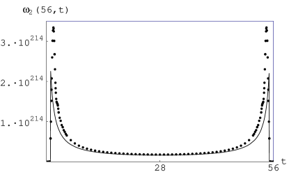
Figure 1: $\omega_{2}(56,t)$ computed numerically. The continuous line represents $\omega_{2}$ as given by using $\Omega_{1}^{h}$ only ($\alpha^{\prime}=1$).

4.1 The calculation of Brandenberger and Vafa revisited

Taking into account that $\Omega\left(E\right)=\sum_{n=0}^{\infty}\Omega_{n}\left(E\right)$, and using (6), for the single string density of states when $E>\Lambda$, Brandenberger and Vafa obtained

$$\qquad\Omega^{\,h}\left(E\right)=\frac{\mathrm{e}^{\beta_{H}E}}{2\pi E}\int_{-\infty}^{\infty}\mathrm{d}\alpha\,\mathrm{e}^{-\mathrm{i}\alpha}\,\mathrm{e}^{\,\int_{\frac{\Lambda}{E}}^{1}\frac{\mathrm{d}x}{x}\mathrm{e}^{\mathrm{i}\alpha x}}=\frac{\mathrm{e}^{\beta_{H}E}}{\Lambda}\left(a+b\,\frac{\Lambda}{E}\right)$$ (15)

where:

$$a = \frac{1}{2\pi}\int_{-\infty}^{\infty}\mathrm{d}\alpha\,\mathrm{e}^{\,\int_{0}^{\alpha}\mathrm{d}x\frac{\cos{x}-1}{x}}\,\cos{\left(\int_{0}^{\alpha}\mathrm{d}x\frac{\sin{x}}{x}-\alpha\right)}=0.56\pm 0.01$$

$$b = \frac{1}{2\pi}\int_{-\infty}^{\infty}\alpha\,\mathrm{d}\alpha\,\mathrm{e}^{\,\int_{0}^{\alpha}\mathrm{d}x\frac{\cos{x}-1}{x}}\sin{\left(\int_{0}^{\alpha}\mathrm{d}x\frac{\sin{x}}{x}-\alpha\right)}=-0.29\pm 0.01$$

The values of $a$ and $b$ were calculated numerically. Note that, although the exponent gives, when $\alpha\gg 1$, a factor $-\log\alpha$, the second integral is not convergent because of the oscillatory behavior of the integrand, and so it has to be regulated and they did it by using an exponentially decaying factor. The sign of $b$ produces a positive specific heat, and the Hagedorn temperature is then a maximum one in the microcanonical ensemble. We think, nevertheless, that this scenario needs a revision: there is nothing a priori unphysical in negative specific heats in the microcanonical ensemble, and anyhow, we are not sure that there could be a positive specific heat phase in the microcanonical ensemble for the gas of strings with windings and momenta.

In fact, it is easy to see how a contradiction appears, when $b=-0.29$, in the following way: using (15) and the fact that $Z\left(\beta\right)={\cal{L}}\left\{\Omega\left(E\right)\right\}$ the following expression for the partition function can be obtained:

$$Z^{\,h}\left(\beta\right)=\frac{a\,\mathrm{e}^{-\left(\beta-\beta_{H}\right)\phi}}{\Lambda\left(\beta-\beta_{H}\right)}+b\,\Gamma\left[0,\phi\left(\beta-\beta_{H}\right)\right]$$ (16)

whereas from the single density of states it is possible to arrive also to an expression for the multiple string partition function via the equality $-\beta F\left(\beta\right)={\cal{L}}\left\{\Omega_{1}\left(E\right)\right\}$

$$Z^{\,h}\left(\beta\right)=\mathrm{e}^{-\beta F\left(\beta\right)}=\frac{\mathrm{e}^{-\gamma}}{\Lambda\left(\beta-\beta_{H}\right)}+\mathrm{e}^{-\gamma}+\mathrm{O}\left[\left(\beta-\beta_{H}\right)^{1}\right]$$ (17)

Comparing (16) and (17), one immediately gets that $a=\exp{\left(-\gamma\right)}=0.5614$, which perfectly agrees with the numerical value given in [1]. But it is a very notorious fact that in (17) no term is found analogous to the logarithmically divergent one hidden in the incomplete gamma function of (16).

Furthermore, we have found an alternative calculation where the coefficient $b$ is actually zero and then, only one divergent term is present in both equations (16) and (17). As it is written in (6), the high energy dominant term in the single string density of states has a dimensionless factor which equals unity in the type II and the heterotic string (this factor could be volume dependent when considering open strings and branes). However, it is very useful to introduce in $\Omega_{1}\left(E\right)$ a factor $c$ that could be thought just as a regulator (whereas we are going to give it a physical meaning at the end of this subsection). This change adds a factor $c^{n}$ to $\Omega_{n}$ in (14). Only at the end the limit $c$ approaching to one will be taken. Furthermore, it is possible to work out the values of $a$ and $b$ analytically if a simple change is made in (14): the key ingredient is noting that the upper limit in the integrals can be taken to infinity since the Dirac delta function ensures that no value greater than $E$ will contribute to them. This will render the final integrals much easier to perform; then, we will have

$$\int_{\Lambda}^{E}\mathrm{d}E_{i}\longrightarrow\int_{\Lambda}^{+\infty}\mathrm{d}E_{i}\qquad\Rightarrow\qquad\Omega^{\,h}\left(E\right)=\frac{\mathrm{e}^{\beta_{H}E}}{2\pi E}\int_{-\infty}^{+\infty}\mathrm{d}\alpha\,\mathrm{e}^{-\mathrm{i}\alpha}\,\mathrm{e}^{c\int_{\frac{\Lambda}{E}}^{\infty}\frac{\mathrm{d}x}{x}\mathrm{e}^{\mathrm{i}\alpha x}}$$ (18)

The calculation is now analogous to the one made in [1], taking the first terms in the series expansion in $\Lambda/E$.

$$\Omega^{\,h}\left(E\right) = \frac{\mathrm{e}^{\beta_{H}E}}{2\pi E}\int_{-\infty}^{+\infty}\mathrm{d}\alpha\,\mathrm{e}^{-\mathrm{i}\alpha}\,\mathrm{e}^{c\int_{\frac{\alpha\Lambda}{E}}^{\infty\cdot\mathrm{sg}\left(\alpha\right)}\frac{\mathrm{d}x}{x}\cos{x}}\,\mathrm{e}^{\mathrm{i}c\int_{\frac{\alpha\Lambda}{E}}^{\infty\cdot\mathrm{sg}\left(\alpha\right)}\frac{\mathrm{d}x}{x}\sin{x}}$$ (19)

$$= \frac{\mathrm{e}^{\beta_{H}E}}{2\pi E}\int_{-\infty}^{+\infty}\mathrm{d}\alpha\,\mathrm{e}^{-c\cdot\mathrm{Ci}\left(\frac{\alpha\Lambda}{E}\right)}\,\cos\left(\alpha+c\cdot\mathrm{si}\left(\frac{\alpha\Lambda}{E}\right)\right)$$

Where $\mathrm{sg}\left(\alpha\right)$ stands for the sign function. It is important to note that the $\mathrm{Ci}$ and the $\mathrm{si}$ functions only coincide with the standard cosine integral and sine integral functions for positive values of $\alpha$. $\mathrm{Ci}\left(x\right)$ is a real, even function of $x$ whereas $\mathrm{si}\left(x\right)$ is a real, odd function of its argument with a discontinuity at $x=0$ and $\mathrm{si}\left(0\right)=0$. This is easy to understand as a consequence of the integral upper limits including the $\mathrm{sg}\left(\alpha\right)$ term in the exponential factors in (19). The integrand is then even and one could perform a series expansion in terms of $\alpha\Lambda/E$. Approximating $\mathrm{Ci}\left(\frac{\alpha\Lambda}{E}\right)=\gamma+\log\left(\frac{\alpha\Lambda}{E}\right)+\mathrm{O}\left(\frac{\alpha\Lambda}{E}\right)$ and $\mathrm{si}\left(\frac{\alpha\Lambda}{E}\right)=\frac{-\pi}{2}+\frac{\alpha\Lambda}{E}+\mathrm{O}\left(\frac{\alpha\Lambda}{E}\right)^{2}\,(\alpha>0)$, we arrive at

$$\Omega^{\,h}\left(E\right)=\mathrm{e}^{-\gamma}\,\frac{\mathrm{e}^{\beta_{H}E}}{\pi E}\,\left(\frac{E}{\Lambda}\right)^{c}\int_{0}^{\infty}\frac{\mathrm{d}\alpha}{\alpha^{c}}\cos\left(\alpha-c\frac{\pi}{2}+c\frac{\alpha\Lambda}{E}\right)$$ (20)

Using that $\cos\left(a-b\right)=\cos a\cos b+\sin a\sin b$ and taking the lowest order in $\alpha\Lambda/E$ one finally gets

$$\Omega^{\,h}\left(E\right)=\frac{E^{c-1}}{\Lambda^{c}}\,\mathrm{e}^{\beta_{H}E}\left[a(c)+b(c)\,\frac{\Lambda}{E}+\mathrm{O}\left(\frac{\Lambda}{E}\right)^{2}\,\right]$$ (21)

$$a\left(c\right) = \frac{\mathrm{e}^{-c\gamma}}{\pi}\int_{0}^{\infty}\frac{\mathrm{d}\alpha}{\alpha^{c}}\cos\left(\frac{c\pi}{2}-\alpha\right)=\frac{\mathrm{e}^{-c\gamma}}{\Gamma\left(c\right)}\qquad\mbox{if $0<c<1$}$$

$$b\left(c\right) = \frac{c\,\mathrm{e}^{-c\gamma}}{\pi}\int_{0}^{\infty}\frac{\mathrm{d}\alpha}{\alpha^{c-1}}\sin\left(\frac{c\pi}{2}-\alpha\right)=\frac{c\,\mathrm{e}^{-c\gamma}}{\Gamma\left(c-1\right)}\qquad\mbox{if $1<c<2$}$$

The integrals converge only for the indicated values of $c$. Clearly, in the $c\rightarrow 1$ limit, the result for $a$ is fully compatible with the numerical value given in [1]; the problem is that it is very easy to see how in this limit $b$ goes to zero. As a matter of fact this method can be generalized and more terms of the form $d_{n}\left(\Lambda/E\right)^{n}\,(n\in\mathbb{N})$ can be computed, giving all of them zero for $d_{n}$ in the $c\rightarrow 1$ limit.

Now, it is straightforward to see how the contradiction between the equations analogous to (16) and (17), that now depend on $c$, has disappeared. Using $\Omega_{1}\left(E\right)=c\,\mathrm{e}^{\beta_{\scriptscriptstyle H}E}/E$ we have that

$$Z^{\,h}\left(\beta\right)=\mathrm{e}^{-c\,\beta F^{\,h}\left(\beta\right)}\approx\frac{\mathrm{e}^{-c\,\gamma}}{\Lambda^{c}\left(\beta-\beta_{H}\right)^{c}}+\frac{c\,\mathrm{e}^{-c\,\gamma}}{\Lambda^{c-1}\left(\beta-\beta_{H}\right)^{c-1}}+\mathrm{O}\left(\left(\beta-\beta_{H}\right)^{2-c}\right).$$ (22)

And making directly the Laplace transform of (21), the same expression for $Z\left(\beta\right)={\cal{L}}\left\{\Omega\left(E\right)\right\}$ can be found for $c>1$. When $c=1$ an annoying constant term appears preventing us to fix more than the only divergent term.

Once the value $c=1$ is taken, the expression for the density of states of the string gas in a finite size container is given by

$$\Omega^{\,h}\left(E\right)=\mathrm{e}^{-\gamma}\,\frac{\mathrm{e}^{\beta_{H}E}}{\Lambda}\qquad E\gg\Lambda.$$ (23)

From this we can calculate both the entropy of the system and its temperature. The fundamental thermodynamic relationship giving the entropy as a function of the energy now looks like

$$S^{h}\left(E\right)=\beta_{H}E+\log\left(\frac{\mathrm{e}^{-\gamma}}{\Lambda}\right).$$ (24)

Comparing it with (10), the analogous expression in the fixed temperature, case we see how both ensembles seem to be inequivalent as pointed in (8). With this entropy we will also have that temperature is fixed to Hagedorn’s, and we would have to conclude that $C_{V}\left(E\right)$ would be infinite.

The constant $c$ has been introduced as a mere way of doing analytical continuation of ill-defined expressions, but we can give it a physical interpretation. Lets look at the expression defining $\Omega\left(E\right)$ once $c$ is introduced

$$\Omega\left(E\right)=\sum_{n=0}^{\infty}c^{n}\,\Omega_{n}\left(E\right)$$ (25)

We see that $c$ is really acting as the fugacity of the system, so that working with a generic value of $c$ and then performing the $c\rightarrow 1$ limit is exactly the same as working with a generic non null chemical potential and then taking it to zero. This interpretation also lets us know that we have not been working in the microcanonical ensemble, but in the ”enthalpic” one [2] for which energy and the chemical potential are given. This way $\Omega\left(E\right)$ now depends on $c$ and becomes $\Omega\left(E,c\right)$.

4.2 Fluctuations for the fixed energy description

It is now clear that the density of states of the string gas is given by

$$\Omega^{\,h}\left(E\right)=\frac{\mathrm{e}^{-\gamma}}{\Lambda}\,\theta\left(E-\phi\right)\,\mathrm{e}^{\beta_{\scriptscriptstyle{H}}\,E}$$ (26)

The multi-string energy cutoff $\phi$ cannot be completely determined without matching the high energy regime with the low energy phase because, imposing that $\beta F^{\,h}\left(\beta\right)$ must be obtained, $\phi$ would appear as a factor of $\left(\beta-\beta_{H}\right)^{\,0}$ that is a regular term being $F^{l}\left(\beta\right)$ also regular at $\beta_{H}$. The matching can be done, but we are not going to dwell further on this point.

An immediate consequence of (24) is that the high energy microcanonical specific heat, $C_{V}^{\,h}\left(E\right)$, is divergent contrary to what, by using [1], has been assumed as true for more than fifteen years.

Once $\Omega\left(E,c\right)$ for the enthalpic ensemble is obtained, it is straightforward to compute the number of strings and its fluctuations as

$$\begin{split}\overline{N}\left(E\right)&=\left.c~{}\partial_{c}\log\Omega\left(E,c\right)\right|_{c=1}\approx\log\left(\frac{E}{\Lambda}\right)\\ \frac{\sqrt{\overline{\Delta N^{2}}\left(E\right)}}{\overline{N}\left(E\right)}&=\frac{\sqrt{\left.\left(c~{}\partial_{c}\right)^{2}\log\Omega\left(E,c\right)\right|_{c=1}}}{\overline{N}\left(E\right)}\approx\frac{1}{\sqrt{\overline{N}\left(E\right)}}\end{split}$$

with

$$\begin{split}\Omega^{\,h}\left(E,c\right)=\theta\left(E-\phi\right)\frac{\mathrm{e}^{\,-c\gamma}}{\Lambda^{\,c}\Gamma\left(c\right)}&E^{\,c-1}\mathrm{e}^{\beta_{\scriptscriptstyle{H}}E}\,\\ &\left[1+\left(c-1\right)\,\mathrm{O}\left(\frac{\Lambda}{E}\right)+...\right]\end{split}$$ (27)

that has been obtained by Laplace inversion of $\mathrm{e}^{\,c\,q\left(\beta\right)}$.

4.3 Other refinements

In the preceding sections any dependence on $R$ has been lost as a result of being in a physical situation in which sums can be well approximated by integrals. Now, we would like to add the effects of introducing Euler-Maclaurin corrections [4] in the integrals that represent sums over windings and momenta. This can also be done by means of a Poisson resummation. As a result, there appear more singular points in $-\beta F\left(\beta\right)$ whose location depends on $R$ [11].

$$-\beta F^{\,h}\left(\beta\right)=\sum_{\vec{m},\vec{n},j}\,\Gamma\left[0,\frac{2\pi\,\left(\beta^{\,2}-\beta_{\vec{m},\vec{n},j}\left(R\right)^{\,2}\right)}{\epsilon\beta_{H}^{\,2}}\right]$$ (28)

with

$$\beta^{\,2}_{\vec{m},\vec{n},j}=\frac{\alpha^{\prime}\pi^{\,2}}{\left(j+1/2\right)^{\,2}}\,\left[2-\frac{R^{\,2}}{\alpha^{\prime}}\vec{m}^{\,2}-\frac{\alpha^{\prime}}{R^{\,2}}\vec{n}^{\,2}\right]$$ (29)

Assuming $R>\sqrt{\alpha^{\prime}}$ the singularity nearest to $\beta_{\scriptscriptstyle{H}}$ is $\beta_{1}=\beta_{\scriptscriptstyle{H}}-\eta$, $\eta\approx\alpha^{\prime}\beta_{\scriptscriptstyle{H}}/(4R^{\,2})$. Considering also the term depending on $\beta_{1}$ we get a corrected expression for the density of states

$$\Omega^{\,h}\left(E,R\right)=\frac{\mathrm{e}^{-\gamma}}{\Lambda}\,\theta\left(E-\phi\right)\,\mathrm{e}^{\beta_{\scriptscriptstyle{H}}\,E}\left(1-\frac{\mathrm{e}^{-\eta E}\left(\eta E\right)^{17}}{\Gamma\left(18\right)}\right)\left(\frac{\mathrm{e}^{-\gamma}}{2\eta\Lambda}\right)^{\,18}$$ (30)

Where $\eta E\gg 1$ has been assumed. This expression depends on $R$ through $\eta$ and the $R$ corrections are actually non extensive. If taken into account, the effect of these corrections on $\beta$ would be

$$\beta\left(E\right)=\beta_{H}+\eta\frac{\mathrm{e}^{-\eta E}}{\Gamma\left(18\right)}\,\left(\eta E\right)^{17}$$ (31)

The second term on the right hand side of this expression has already been studied in the literature [11], [12] and has been frequently claimed as being the cause of having a positive specific heat. It is easy to see that, after all, having enough energy for a given radius, the gas can always be in the regime in which there is no dependence on the volume and this is the regime of the Brandenberger-Vafa scenario, for which the specific heat diverges. The radius corrections are exponentially suppressed and, for our system, are not different from the finite volume corrections that are dropped when the thermodynamic limit is taken over the ideal gas of particles (see, for example, [2]).

5 Conclusions

As a first important result, it is crucial to remark that no published calculation has found the $-0.29\,\,\mathrm{e}^{\beta_{H}\,E}/E$ term but the one presented by Brandenberger and Vafa in [1]. This is the term that is needed to state, as these authors do, that the microcanonical specific heat is positive in the physical situation in which energy density is so high that the density of states does not depend on the volume. As far as we know, what any other calculation actually gets is that, for the same physical situation, the specific heat is divergent because a null $b$ coefficient is found (see eq. (15)). In reference [11], it is explicitly admitted that $b=-0.29$ is not found, but the authors do not face the important question that the contradiction between their calculation and that of Brandenberger and Vafa rises. It seems that this is so because they consider they are using what they call a different ”formalism”. In our work, we clearly show that, using the same technique Brandenberger and Vafa used and a physically meaningful regularization, the $b$ coefficient vanishes (and also any other high energy correction). This is the first result of our work and, in our opinion, critically depends on understanding that the ”micro” ensemble is really the ”enthalpic” one, namely, a fixed energy and fixed chemical potential ensemble.

We have used the $S$-representation of the Helmholtz free energy to finally conclude that the behavior of the free energy around $\beta_{H}$ coincides with what is gotten from the $F$ representation. This might be expected but it is not a trivial fact, because both representations do not coincide. That the $S$ and $F$ representations are not equal seems to be clearly commented for the first time in [13]. The relationship between both representations is carefully studied for the family of the heterotic strings in [14] (see also [15]). In those works it is clearly established that the $F$-representation does not provide an analytical function for complex $\beta$. In other words, it is false that the $F$-representation can be seen as providing the analytical continuation of the $S$-representation for heterotic strings. Then, it is not rigorous to say that the $F$-representation of the free energy can be used to get the density of states by inverse Laplace transformation of the corresponding partition function. What one can only do is to continue the $S$-representation. When one uses the $F$-representation to get the behavior around $\beta_{H}$ one is really using it in the interval $(\beta_{H},+\infty)$ where it coincides with the $S$-representation. Now, we are also providing a very concrete and explicit example of to what extent the $S$ and $F$ representations of the free energy are equal.

From other point of view, taking into account that the $F$-representation gives the free energy as computed for the compactification of the Euclidean time on a circle of length $\beta$ (including string windings along it), in [16] there appears a proof for the noncritical $c=1$ string of the recently emphasized fact that, for strings, the free energy cannot be computed, at any temperature, by the compactification of time [17].

Another important point is to what extent the $R$ corrections presented in subsection (4.3) can be taken as showing that the system really has a positive specific heat. This seems to be the belief as expressed in [11] and [12]. In our opinion, the problem is that these nonextensive corrections are exponentially suppressed with the value of the energy and are then of no thermodynamical relevance for the system in the thermodynamical limit in which the energy density is very high and the sum over windings and momenta can be replaced by an integral. Those corrections are as the finite volume $1/\sqrt{V}$ corrections for the gas of free particles; they are irrelevant in the thermodynamical limit in which the sum over momenta can be replaced by an integral.

In the case we treat the gas in the fixed temperature (canonical) description, the big fluctuations might justify the exclusion of the nonextensive term that renders the canonical specific heat positive. In any case, those fluctuations would just make the canonical equilibrium description physically unusable.

From a cosmological point of view, one could think that there would not be any relevant cosmological implication from our results because, after all, the equation of state would still be the same, corresponding to pressureless dust matter ($P=0$). However, things are more intricate because a divergent microcanonical specific heat can be an indication of a phase transition. In our case, what we have done in the microcanonical (really enthalpic) treatment is a description of how the volume of phase space in the N-body problem changes when energy, which is a conserved quantity, increases [18]. We have found that the system behaves very differently from the grand canonical ensemble in which $T_{H}$ would be a maximum temperature and the specific heat, as a function of temperature, would be positive.

What is clear is that a divergent microcanonical specific heat cannot be used ab initio as a criterion to drop as unphysical our gas of closed strings at finite size.

A. The UV limit in the S-representation partition function

This appendix is devoted to explain how (2) is obtained and to explicitly show that (4) holds.

First of all, the integral computing the sum over windings and momenta can be performed to give

$$\int_{\mathbb{R}^{9}\times\mathbb{R}^{9}}\,\mathrm{d}\vec{l}\,\mathrm{d}\vec{k}\,\mathrm{e}^{-\pi\tau_{2}(\vec{l}^{\,2}+\vec{k}^{\,2})}\mathrm{e}^{2\pi\mathrm{i}\,\vec{l}\cdot\vec{k}\tau_{1}}=\left|\tau\right|^{-9}$$ (A.1)

Next, it has to be noticed that, when $\tau\rightarrow 0$, it holds that

$$\left|\theta_{2}(0,-1/(2\tau))\right|^{\,-16}\approx 2^{\,-16}\,\mathrm{e}^{2\pi\tau_{2}/\left|\tau\right|^{\,2}}$$

because all the other terms are finite when $\tau\rightarrow 0$. One has then to perform the integral over $\tau_{1}$ as providing a function of $\tau_{2}$ given by $\mathrm{e}^{\,2\pi/\tau_{2}}$ times a series expansion in powers of $\tau_{2}$ as it appears on the right hand side of (2). Namely, the left hand side of (2) (we called it $I(\tau_{2})$) is now given by

$$\begin{split}I(\tau_{2})=\frac{1}{2^{\,8}\tau_{2}}\,\mathrm{e}^{2\pi/\tau_{2}}\,\int_{-1/2}^{+1/2}\,\,\mathrm{d}\tau_{1}\,\,\left(1+\frac{\tau_{1}^{\,2}}{\tau_{2}^{\,2}}\right)^{-1/2}\mathrm{e}^{-2\pi\tau_{1}^{\,2}/\tau_{2}^{\,3}}\,\,\mathrm{e}^{\frac{2\pi}{\tau_{2}\left[1+\tau_{1}^{\,2}/\tau_{2}^{\,2}\right]}-\frac{2\pi}{\tau_{2}}+\frac{2\pi\tau_{1}^{\,2}}{\tau_{2}^{\,3}}}\end{split}$$ (A.2)

It has been written in a way prepared to be rewritten in terms of a function $\tilde{I}(\tau_{2})$ as $I(\tau_{2})=2^{\,-8}\tau_{2}^{\,1/2}\mathrm{e}^{\,2\pi/\tau_{2}}\,\tilde{I}(\tau_{2})$ where

$$\tilde{I}(\tau_{2})=\int_{-\left(2\tau_{2}^{3/2}\right)^{-1}}^{\left(2\tau_{2}^{3/2}\right)^{-1}}\,\mathrm{d}x\,\,\,\mathrm{e}^{-2\pi x^{\,2}}\,\mathrm{e}^{\frac{2\pi}{\tau_{2}}\left[\frac{1}{1+x^{\,2}\tau_{2}}-\left(1-\tau_{2}x^{\,2}\right)\right]}\left(1+\tau_{2}x^{\,2}\right)^{-1/2}$$ (A.3)

For which the change of variables $\tau_{1}=x\,\tau_{2}^{3/2}$ has been used. Now, for the product of the last two factors in the integrand, the following series expansion can be written

$$\begin{split}\mathrm{e}^{\frac{2\pi}{\tau_{2}}\left[\frac{1}{1+x^{\,2}\tau_{2}}-\left(1-\tau_{2}x^{\,2}\right)\right]}&\left(1+\tau_{2}x^{\,2}\right)^{-1/2}=\mathrm{e}^{2\pi x^{\,4}\tau_{2}/(1+\tau_{2}x^{\,2})}\left(1+\tau_{2}x^{\,2}\right)^{-1/2}\\ \ &=\sum_{b=0}^{+\infty}\,\sum_{a=0}^{+\infty}\,\,\frac{(-1)^{\,a}(2\pi)^{\,b}\,\Gamma\left(b+a+1/2\right)\,}{b!\,\,a!\,\,\Gamma\left(b+1/2\right)}\,\tau_{2}^{\,b+a}\,x^{\,4b+2a}\end{split}$$ (A.4)

Next we are able to perform the integral over $x$ of the term $x^{4b+2a}$ obtaining

$$\begin{split}\int_{-\left(2\tau_{2}^{3/2}\right)^{-1}}^{\left(2\tau_{2}^{3/2}\right)^{-1}}\,\mathrm{d}x\,\mathrm{e}^{-2\pi x^{\,2}}\,x^{4b+2a}&=\frac{\Gamma\left(2b+a+1/2\right)-\Gamma\left(2b+a+1/2,2\pi/(4\tau_{2}^{\,3})\right)}{(2\pi)^{2b+a+1/2}}\\ &\approx(2\pi)^{-2b-a-1/2}\,\Gamma\left(2b+a+1/2\right)\end{split}$$ (A.5)

where the last approximation results from the exponential suppression of the contribution coming from the incomplete Gamma function when its argument gets big (what happens here when $\tau_{2}\rightarrow 0$).

Now one of the sums in the resulting double sum to get $\tilde{I}$ can be calculated (!!) to finally give

$$\tilde{I}(\tau_{2})=\sum_{b=0}^{+\infty}\,(2\pi)^{-b-1/2}\,\Gamma\left(b+1/2\right)\,\tau_{2}^{\,b}$$ (A.6)

We are then able to get $I(\tau_{2})$ and, in particular, the coefficients $a_{i}$ as

$$a_{i}=\frac{\Gamma\left(i+1/2\right)}{(2\pi)^{\,i}\sqrt{\pi}}$$ (A.7)

The next step is to use $I(\tau_{2})$ as written in (2) with the already known $a_{i}$ coefficients to compute $F^{\,h}(\beta)$ finding then the $b_{n}$ factors in (3). This is easily done to give

$$b_{n}=(-1)^{\,n}\,\frac{a_{n}}{\beta_{H}\,n!}$$ (A.8)

The final computation is that of the series generated by the $b_{n}$ coefficients as it appears on the left hand side of (4), namely

$$R(\beta)\equiv\sum_{n=0}^{+\infty}\,b_{n}\left(\beta^{\,2}-\beta_{H}^{\,2}\right)^{n}\left(\frac{2\pi}{\beta_{H}^{\,2}}\right)^{n}$$ (A.9)

Taking into account that $\beta^{2}-\beta_{H}^{\,2}=2\beta_{H}\left(\beta-\beta_{H}\right)\left(1+\frac{\beta-\beta_{H}}{2\beta_{H}}\right)$, $R(\beta)$ can be written as a double sum

$$R(\beta)=\sum_{n=0}^{+\infty}\,\left[\frac{1}{\sqrt{\pi}}\,\sum_{q=0}^{n}\,\frac{(-1)^{\,q}\,2^{\,2q-n}\Gamma\left(q+1/2\right)}{\left(n-q\right)!\left(2q-n\right)!}\right]\,\,\frac{\left(\beta-\beta_{H}\right)^{n}}{\beta_{H}^{\,n+1}}$$ (A.10)

The term between square brackets can be computed to give exactly $(-1)^{\,n}$. So, we have finally showed that

$$R(\beta)=1/\beta$$ (A.11)

by showing that it is given by the power series expansion of $1/\beta$ around $\beta_{H}$.

References

- [1] R. Brandenberger and C. Vafa, Nucl. Phys. B 316 (1989) 391.
- [2] M. A. Cobas, M. A. R. Osorio, M. Suárez, Phys. Lett. B 601 (2004) 99.
- [3] E. Álvarez, M. A. R. Osorio, Phys. Rev. D 36 (1987) 1175.
- [4] M. A. Cobas, M. A. R. Osorio, M. Suárez, ”Educing the volume out of the phase space boundary”, hep-th/0211211.
- [5] P. Salomonson, B. Skagerstam, Nucl. Phys. B 268 (1986) 349.
- [6] M. A. Cobas, M. A. R. Osorio, M. Suárez, ”Exotic fluids made of open strings”, hep-th/0411265.
- [7] T. L. Hill, ”Statistical Mechanics. Principles and selected applications”, Dover Publications Inc., New York , 1987.
- [8] H. Touchette, Equivalence and Nonequivalence of the Microcanonical and Canonical Ensembles: A Large Deviations Study, Ph. D. Thesis (2003), McGill University.
- [9] M. Laucelli Meana, J. Puente Peñalba, M. A. R. Osorio, Phys. Lett. B 400 (1997) 275.
- [10] S. Frautschi, Phys. Rev. D 3, 2821 (1971).
- [11] N. Deo, S. Jain and C.-I. Tan, Phys. Lett.. B 220 (1989) 125.
- [12] S. A. Abel, J. L. F. Barbón, I. I. Kogan, E. Rabinovici, JHEP 9904 (1999) 015.
- [13] D. Kutasov, N. Seiberg, Nucl. Phys. B 358 (1991) 600.
- [14] M. A. R. Osorio, M. A. Vázquez-Mozo, Phys. Rev. D 47 (1993) 3411.
- [15] M. A. R. Osorio, M. A. Vázquez-Mozo, Phys. Lett. B 280 (1992) 21.
- [16] M. A. R. Osorio, M. A. Vázquez-Mozo, Mod. Phys. Lett. A 8 (1993) 3215.
- [17] J. L. Davis, F. Larsen, N. Seiberg, JHEP 0508 (2005) 035.
- [18] D. H. E. Gross, Microcanonical thermodynamics: Phase transitions in ”small” systems, Lecture Notes in Physics, Vol. 66, World Scientific, Singapore, 2001; ”Heat can flow from cold to hot in Microcanonical Thermodynamics of finite systems. The microscopic origin of condensation and phase separations”, cond-mat/0409542.