Stringy Derivation of Nahm Construction of Monopoles

Abstract:

We derive the Nahm construction of monopoles from exact tachyon condensation on unstable D-branes. The Dirac operator used in the Nahm construction is identified with the tachyon profile in our D-brane approach, and we provide physical interpretation of the procedures Nahm gave. Crucial is the introduction of infinite number of brane-antibranes from which arbitrary D-brane can be constrcuted, exhibitting a unified view of various D-branes. We explicitly show the equivalence of the D3-brane boundary state with the monopole profile and the D1-brane boundary state with the Nahm data as transverse scalars.

1 Introduction and Summary of the Derivation

D-branes, owing to their variety in dimensions and protean shapes, provide new accesses to nonperturbative aspects in field theories. In particular, solitons in field theories often admit stringy interpretation, which enables one to view them as geometric objects: compound branes in higher dimensions. Once the corresponding brane configuration is identified, one can make various stringy deformations/dualities ending up with new perspectives on the solitons. For example, different kinds of D-branes are related and equivalent, especially through tachyon condensation [1] describing creation/annihilation of D-branes. For a demonstration of the powerfulness of the D-brane technique, study of instantons/monopoles is appropriate due to their obvious importance. In this article, we derive completely the Nahm’s construction of BPS monopoles [2, 3], using a D-brane technique in string theory — exact tachyon condensation. For the derivation we apply the idea of K-matrix theory [4, 5] in which any species of D-branes can be described by the tachyon condensation of infinite number of a single kind of D-branes and anti-D-branes.

Brane configuration of $k$ BPS monopoles in SU($N$) super Yang-Mills theory is composed of $k$ D-strings (D1-branes) suspended between parallel $N$ D3-branes (Fig.1) in type IIB superstring theory. Evidence for this correspondence is through identification of masses, charges and supersymmetries preserved [6]. The equations for the monopole

$$D_{i}\Phi=\frac{i}{2}\epsilon_{ijk}F_{jk}\,\quad(i,j,k=1,2,3)$$ (1.1)

can be viewed as BPS equations in the effective field theory on the D3-branes. The brane interpretation made it possible to predict existence of generalized monopoles, such as monopoles in noncommutative spaces [7] and 1/4 BPS dyons [8], whose explicit field configurations were obtained later accordingly [9, 10]. In the Nahm’s method, arbitrary BPS monopoles can be constructed through definite procedures starting with solving Nahm’s equations

$$\partial_{\xi}T_{i}(\xi)=i\epsilon_{ijk}T_{j}(\xi)T_{k}(\xi)$$ (1.2)

to get their $k\times k$ matrix solutions $T_{i}(\xi)$ called Nahm data, as briefly reviewed below. It was shown by Diaconescu [11] that the Nahm’s equations are in fact BPS equations in the worldvolume effective theory on the D-strings. These already exhibit how powerful the D-brane technique is, but it was not enough, since D-brane interpretation of the Nahm’s construction itself has not been revealed, except for the partial derivation by the probe analysis [11]. We shall show that in fact all the procedures Nahm provided for the construction have stringy physical interpretation in higher dimensions, and resultantly derive the Nahm’s monopole construction which was obtained originally from ADHM construction [12].

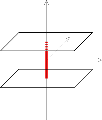
Figure 1: A schematic picture of the brane configuration corresponding to typical BPS monopoles in SU(2) super Yang-Mills theory.

Nahm argued [2] that, with the solutions to the equations (1.2) in a period $\xi\in(-a,a)$ with a certain boundary condition, normalizable wave functions ${\left\langle\xi\right|}\rho,x^{i}\rangle$ of the “Dirac operator” (in one dimensional space spanned by $\xi$)

$$\nabla\equiv\hbox to3.8pt{\hskip 1.3pt\vrule height=7.4pt,width=0.4pt\hskip 0.7pt\vrule height=7.85pt,width=0.4pt\kern-2.4pt\hrulefill\kern-3.0pt\raise 3.7pt\hbox{\char 32\relax}}_{2k\times 2k}\frac{\partial}{\partial\xi}+i\sigma_{i}\otimes(x^{i}\hbox to3.8pt{\hskip 1.3pt\vrule height=7.4pt,width=0.4pt\hskip 0.7pt\vrule height=7.85pt,width=0.4pt\kern-2.4pt\hrulefill\kern-3.0pt\raise 3.7pt\hbox{\char 32\relax}}_{k\times k}-T_{i}(\xi)),\qquad\nabla{\left|\rho,x^{i}\right\rangle}=0\quad(\rho=1,2,\cdots,N)\quad$$ (1.3)

provide monopole field profiles by the formula

$$\Phi(x^{i})_{\rho\rho^{\prime}}\equiv{\left\langle\rho,x^{i}\right|}\xi{\left|\rho^{\prime},x^{i}\right\rangle},$$ (1.4)

$$A_{i}(x^{j})_{\rho\rho^{\prime}}\equiv{\left\langle\rho,x^{j}\right|}\frac{\partial}{\partial x^{i}}{\left|\rho^{\prime},x^{j}\right\rangle}.$$ (1.5)

To derive these full procedures in string theory, we resort to the idea of tachyon condensation which provides a unified viewpoint of the D3-branes and the D-strings. The K-matrix theory [4] ensures that infinite number of D$p$-branes and anti-D$p$-branes (or non-BPS D$p$-branes) can reproduce any kind of D-branes, and since we are interested in monopoles living on the D3-brane worldvolume theory, let us start with infinite number of parallel D3-branes and anti-D3-branes along the $x^{i}$ directions. To see the relation to the D-string picture on which the Nahm data is realized [11], we consider on the D3-branes a tachyon condensation representing the D-strings. The D-string worldvolume direction $\xi$ is orthogonal to the worldvolume direction of the D3-brane $(x^{1},x^{2},x^{3})$, thus we are inevitably lead to introduce non-BPS D4-branes whose worldvolume spans $(x^{1},x^{2},x^{3},x^{4}\equiv\xi)$, as an intermediate step. See Fig.2(Left) in which the dashed box is the non-BPS D4-branes (on top of each other). Once we construct the non-BPS D4-branes from the D3-branes by the tachyon condensation, then we further make another tachyon condensation to realize the D-strings, as in Fig.2(Right). Therefore the tachyon condensation is a sequence

$$\left(\begin{array}[]{c}\mbox{D3-branes}\\ \mbox{anti-D3-branes}\end{array}\right)\quad\rightarrow\quad\mbox{non-BPS D4-branes}\quad\rightarrow\quad\mbox{D-strings}.$$ (1.8)

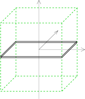
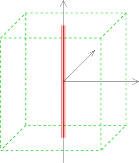
Figure 2: Left: D3-branes and anti-D3-branes are shown in solid planes, while the dashed box represents non-BPS D4-branes. Right: Solid lines are D-strings made out of the non-BPS D4-branes (the dashed box) by the tachyon condensation.

Although schematically the brane configuration corresponding to the monopoles is Fig.1, the actual configuration looks like Fig.3. The worldvolumes of the D3-branes are curved due to the excitation of the transverse scalar field $\Phi(x^{i})$. There is another way of interpreting the picture of Fig.3: by turning on the transverse scalar fields $T_{i}(\xi)$ on the D-strings of Fig.2(Right), the desired brane configuration Fig.3 can be constructed, in which the D-string worldvolume is expanded into 4 dimensions via renowned Myers’ effect [13]. This Myers’ effect occurs for mutually-noncommutative matrix transverse fields on the D-strings, which is manifested in the Nahm’s equation (1.2). In summary, to produce the brane configuration Fig.3, we have two ways —

• The D3-branes with the monopole field configuration which should be a direct interpretation of the starting entry of the sequence (1.8).

• The expanded D-strings with the Nahm data, the end point of the sequence (1.8).

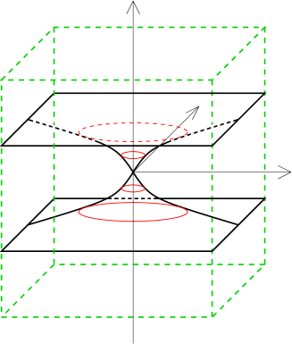
Figure 3: The actual brane configuration representing the BPS monopoles in the SU(2) gauge theory.

Let us see the tachyon condensation (1.8) in a little more detail. The second arrow in (1.8) is so-called D-brane descent relation [1], and it is known that an exact tachyon profile on the non-BPS D4-brane is given [5] by the Atiyah-Bott-Shapiro construction [15],

$$t(\xi,x^{i})=u\sigma_{i}\otimes(x^{i}\hbox to3.8pt{\hskip 1.3pt\vrule height=7.4pt,width=0.4pt\hskip 0.7pt\vrule height=7.85pt,width=0.4pt\kern-2.4pt\hrulefill\kern-3.0pt\raise 3.7pt\hbox{\char 32\relax}}_{k\times k}-T_{i}(\xi)),$$ (1.9)

with the limit $u\rightarrow\infty$ ensuring it to be a classical solution of a boundary string field theory. The last term $T_{i}(\xi)$ is included to give the transverse displacement of the D-strings [14]: the zeros of the tachyon $t$ are the location of the topological defects (the D-strings). To realize the first arrow in the sequence (1.8), we need the D-brane ascent relation [16, 5] in which we prepare infinite number of D3-branes and anti-D3-branes with the following exact tachyon profile [16]

$$T=u\hat{p}_{\xi}+it(\hat{\xi},x^{i}),\qquad\Phi^{4}=\hat{\xi},$$ (1.10)

where again $u\rightarrow\infty$, and $\hat{\xi}$ and $\hat{p}_{\xi}$ are the infinite dimensional matrix representation of the Heisenberg algebra $[\hat{\xi},\hat{p}_{\xi}]=i$. The anti-hermite part of $T$ becomes the real tachyon on the non-BPS D4-branes. Therefore, altogether, on the D3-branes and anti-D3-branes, if we turn on the tachyon profile (1.10) and (1.9), we obtain the desired D-string configuration with the Nahm data $T_{i}(\xi)$. This is the realization of the sequence (1.8):

$$T=u\hat{p}_{\xi}+iu\sigma_{i}\otimes(x^{i}\hbox to3.8pt{\hskip 1.3pt\vrule height=7.4pt,width=0.4pt\hskip 0.7pt\vrule height=7.85pt,width=0.4pt\kern-2.4pt\hrulefill\kern-3.0pt\raise 3.7pt\hbox{\char 32\relax}}_{k\times k}-T_{i}(\hat{\xi}))=u\nabla,\qquad\Phi=\hat{\xi}.$$ (1.11)

Quite interestingly, this tachyon is identical to the Dirac operator. The viewpoint $\langle$ii$\rangle$ of the brane configuration Fig.3 through the infinite number of D3-branes and anti-D3-branes naturally gives the physical interpretation of the Dirac operator in the Nahm’s construction.

The derivation of the Nahm’s construction is completed by looking at the interpretation $\langle$i$\rangle$, as we show in the following. We apply the idea of [18]. The consequence of the tachyon profile (1.11) can be seen after it is diagonalized. The divergence of the eigenvalues of the tachyon matrix is directly related to the vanishing of pairs of the D3-brane and the anti-D3-brane. The tachyon potential of the boundary string field theory for the brane-antibrane system [19, 20] is given by ${\rm Tr}\exp[-u^{2}{\cal D}^{2}]\sim{\rm Tr}\exp[-T^{\dagger}T]$ where we have defined a hermitian Dirac operator ${\cal D}\equiv\tiny\left(\begin{array}[]{cc}0&\nabla\\ \nabla^{\dagger}&0\end{array}\right)$. The vanishing of the potential means the disappearance of the D-branes [1]. For the diagonalization we introduce ortho-normalized eigenstates of ${\cal D}$, ${\cal D}{\left|\lambda;x^{i}\right\rangle}=e_{\lambda}{\left|\lambda;x^{i}\right\rangle}$. Then the exponent of the tachyon potential is diagonally expressed as $u^{2}{\cal D}^{2}=\sum_{\lambda}{\left|\lambda,x^{i}\right\rangle}u^{2}e_{\lambda}^{2}{\left\langle\lambda,x^{i}\right|}$. Evidently, entries with $e_{\lambda}\neq 0$ diverges in the limit $u\rightarrow\infty$. Thus only the D3-branes carrying the Chan-Paton index of the zeromode remains, while others vanish.

The location of the infinite number of D3-branes was originally expressed as $\Phi=\hat{\xi}$ as in (1.10). Thus to look at the location of the remaining D3-branes, we just need to see particular matrix elements of $\hat{\xi}$ carrying the zeromode indices. They are given exactly by the Nahm’s formula (1.4), therefore the formula is derived.

The derivation of the formula for the gauge field (1.5) is a little more involved but has a fascinating interpretation: the gauge field is provided as a Berry’s phase. In the reduction to the zeromode states, we thought of them as a function of $x^{i}$, but in string theory $x^{i}$ are worldsheet boundary fields and thus depend on the worldsheet boundary variable $\sigma$ in the path-integral formalism. Therefore the eigenvalue problem of the tachyon field is naturally accompanied by the Berry’s phase,

$$\exp\left[-\oint\!d\sigma\biggm{\langle}\!\!\rho,x^{i}\!\biggm{|}\frac{\partial}{\partial\sigma}\biggm{|}\!\rho^{\prime},x^{i}\!\!\biggm{\rangle}\right]=\exp\left[-\oint\!d\sigma\frac{\partial x^{i}}{\partial\sigma}\biggm{\langle}\!\!\rho,x^{j}\!\biggm{|}\frac{\partial}{\partial x^{i}}\biggm{|}\!\rho^{\prime},x^{j}\!\!\biggm{\rangle}\right].\quad$$ (1.12)

This phase should appear in front of the eigenstate representing the remaining D-branes. Noting that $\partial x^{i}/\partial\sigma$ is nothing but the worldsheet boundary coupling to the background gauge fields, we derive the formula for the gauge fields, (1.5). This completes the stringy derivation of the Nahm’s construction of BPS monopoles. We outlined the derivation here, and its details with the full rigor is given in section 2, in the boundary state formalism with the exact tachyon condensation.

There exists the “inverse” Nahm construction in which for a given monopole field configuration the corresponding Nahm data can be constructed. This inverse construction can also be derived via our D-brane approach, by employing the following new sequence:

$$\left(\begin{array}[]{c}\mbox{D-strings}\\ \mbox{anti-D-strings}\end{array}\right)\quad\rightarrow\quad\mbox{non-BPS D4-branes}\quad\rightarrow\quad\mbox{D3-branes}.$$ (1.15)

For the first arrow we need infinite number of D-strings and anti-D-strings to realize the ascent relation, then the second arrow is the usual co-dimension one domain wall of the tachyon field in the descent relation. It is obvious that the same argument works, and in fact one can derive the inverse Nahm construction.

Originally the Nahm’s construction was obtained [2] by dimensionally reduced ADHM construction of instantons. In view of our derivation, it is almost obvious that the ADHM construction itself can be derived [21] via the tachyon condensation on D4-branes and D0-branes. D-brane realization of the ADHM construction and Nahm transformation has been studied in probe D-brane analyses [22, 17] in background D5-D9-brane systems, but our derivation is direct (in no need of probes) and not in the low energy approximation. Moreover, in our approach, the Nahm construction can be considered as a duality: we can derive the “inverse” Nahm construction in the precisely same manner as the Nahm construction, and the D-strings with the Nahm data and the D3-branes with the monopole profile are treated on an equal footing. Note that even off-shell configurations, which do not satisfy the BPS conditions nor the equations of motion, of the D3-branes and that of the D-strings can be related.

The boundary state formalism with the exact tachyon condensation is so efficient and powerful, and we have no doubt that it will help much for studying generalization/application of the ADHM and Nahm constructions.

2 Detailed Derivation via Boundary States

The equivalence of various D-brane configurations can be most efficiently seen in terms of boundary states. Because boundary states are considered to be by themselves the definition of D-branes, once two boundary states coincide, we can say that those two D-branes are identical. In the derivation of the Nahm’s construction, we make full use of the boundary state formalism. We will show that boundary states of the D-strings and the D3-branes are indeed identical.

Non-BPS D4 $\rightarrow$ D1

First we review the second arrow in the sequence (1.8), that is, the tachyon condensation on the non-BPS D4-branes giving a bunch of D-strings. The final form of the sequence, $k$ static D-strings elongated along $\xi(\equiv x^{4})$ direction with their transverse scalar field $T_{i}(\xi)$ $(i=1,2,3)$, can be represented by the boundary state

$$|B{\rm(D1)}\rangle=\int[d\xi][d\psi^{4}]$$ (2.16)

$$\hskip 14.22636pt\left\{{\rm Tr}{\rm P}\exp\oint d\sigma\left[-\dot{\xi}A_{\xi}(\xi)-iT^{i}(\xi)P_{i}+iD_{i}T^{j}(\xi)\psi^{i}\Pi_{j}-\frac{1}{2}[T^{i}(\xi),T^{j}(\xi)]\Pi_{i}\Pi_{j}\right]\right\}$$

$$\hskip 113.81102pt\times{\left|x^{i}=0,\xi\right\rangle}{\left|\psi^{i}=0,\psi^{4}\right\rangle}.$$

This is in a path-integral representation [23], and the kets are the eigen states of the worldsheet scalar fields, $X^{\mu}(\sigma,\tau)|_{\tau=0}{\left|x^{\mu}(\sigma)\right\rangle}=x^{\mu}(\sigma){\left|x^{\mu}(\sigma)\right\rangle}$. The dot denotes a derivative with respect to the worldsheet boundary variable $\sigma$, $P_{\mu}(\sigma)$ is the conjugate momentum of $X^{\mu}(\sigma)$, and $\Pi_{\mu}(\sigma)$ is that of $\psi^{\mu}(\sigma)$. Tr is the trace over the Chan-Paton indices of the matrices $T_{i}(\xi)$, and the path-ordering P is necessary to ensure the gauge invariance in the target space. Hereafter we take the gauge $A_{\xi}=0$ for simplicity. In this article we don’t explicitly write the overall factor of boundary states and any dependence on directions different from $x^{i}(i=1,2,3)$ and $\xi$ in ten dimensions, for notational simplicity. In this section we set $\alpha^{\prime}=2$, and will argue the $\alpha^{\prime}$ dependence and the low energy limits in the next section.

This boundary state (2.16) can be represented in a different form, by using a descent relation from the non-BPS D4-branes, with the Atiyah-Bott-Shapiro construction [15]. The profile of the tachyon field $t(x^{i},\xi)$ on the non-BPS D4-branes is [14]

$$t=u\sigma_{i}\otimes(x^{i}\hbox to3.8pt{\hskip 1.3pt\vrule height=7.4pt,width=0.4pt\hskip 0.7pt\vrule height=7.85pt,width=0.4pt\kern-2.4pt\hrulefill\kern-3.0pt\raise 3.7pt\hbox{\char 32\relax}}_{k\times k}-T_{i}(\xi)),\qquad u\rightarrow+\infty.$$ (2.17)

This means that we need $2k$ non-BPS D4-branes to produce $k$ D-strings. Here we set $|T_{i}(\xi)|=\infty$ for $|\xi|>a$, which is consistent because of the Nahm’s boundary condition, $|T_{i}(\xi)|=\infty$ at $|\xi|=a$. We need to take the limit $u\rightarrow\infty$ so that the resultant configuration is on-shell, which is shown in the boundary string field theory. The proof of the equivalence of the boundary states follows precisely from the argument in [5]. We write here the non-BPS D4-brane boundary state as a reference,

$${\left|B{\rm(D4)}\right\rangle}=\int[dx^{i}][d\xi][d\psi^{i}][d\psi^{4}]\left\{{\rm Tr}{\rm P}\exp\oint d\sigma\left[-t^{2}\hbox to3.8pt{\hskip 1.3pt\vrule height=7.4pt,width=0.4pt\hskip 0.7pt\vrule height=7.85pt,width=0.4pt\kern-2.4pt\hrulefill\kern-3.0pt\raise 3.7pt\hbox{\char 32\relax}}_{2\times 2}+i\left(\psi^{i}\partial_{i}t+\psi^{4}\partial_{4}t\right)\tau_{1}\right]\right\}$$

$$\hskip 199.16928pt\times{\left|x^{i},\xi\right\rangle}{\left|\psi^{i},\psi^{4}\right\rangle},$$ (2.18)

where $\tau_{i}$ ($i=1,2,3$) are the Pauli matrices. One can show that (2.18) with the tachyon profile (2.17) is identical with (2.16).

D3$\overline{\it D3}$ $\rightarrow$ non-BPS D4

Next, let us consider the first arrow in the sequence (1.8). We represent the non-BPS D4-branes (2.18) in terms of infinite number of D3-branes and anti-D3-branes. The ascent relation follows from the construction in [16], according to which, the profile of the tachyon field $T(x^{i})$ and the transverse scalar field $\Phi(x^{i})$ on infinite number of the D3-branes and the anti-D3-branes is

$$T=u\hat{p}_{\xi}+it(\hat{\xi},x^{i}),\qquad\Phi^{4}=\hat{\xi},\qquad u\rightarrow\infty.$$ (2.19)

Here $\hat{\xi}$ and $\hat{p}_{\xi}$ are matrix representation of the Heisenberg algebra $[\hat{\xi},\hat{p}_{\xi}]=i\hbox to3.8pt{\hskip 1.3pt\vrule height=7.4pt,width=0.4pt\hskip 0.7pt\vrule height=7.85pt,width=0.4pt\kern-2.4pt\hrulefill\kern-3.0pt\raise 3.7pt\hbox{\char 32\relax}}$.

Although straightforward, we explicitly show here that the D3-brane (and anti-D3-brane) boundary state with (2.19) reduces to the non-BPS D4-brane boundary state (2.18), for an instructive purpose. This is a slight generalization of the argument given in [5] where an ascent relation from a non-BPS D$p$-brane to a BPS D$(p\!+\!1)$-brane was shown in the boundary state formalism. We start with the D3-brane anti-D3-brane boundary state [19, 20]

$${\left|{\rm D3}\overline{\rm D3}\right\rangle}=\int[dx^{i}][d\psi^{i}]{\rm Tr}{\rm P}\exp\left[\oint d\sigma M(\sigma)\right]{\left|\xi=0,x^{i}\right\rangle}{\left|\psi^{4}=0,\psi^{i}\right\rangle}$$ (2.20)

where the matrix exponent is given by

$$M(\sigma)\equiv \left[-i\Phi^{4}P_{4}(\sigma)+i\partial_{i}\Phi^{4}\psi^{i}\Pi_{4}\right]\hbox to3.8pt{\hskip 1.3pt\vrule height=7.4pt,width=0.4pt\hskip 0.7pt\vrule height=7.85pt,width=0.4pt\kern-2.4pt\hrulefill\kern-3.0pt\raise 3.7pt\hbox{\char 32\relax}}_{2\times 2}+\left(\begin{array}[]{cc}-TT^{\dagger}&0\\ 0&-T^{\dagger}T\end{array}\right)$$ (2.26)

$$+\left(\begin{array}[]{cc}0&[T,\Phi^{4}]\Pi_{4}+i\partial_{i}T\psi^{i}\\ {}[T^{\dagger},\Phi^{4}]\Pi_{4}+i\partial_{i}T^{\dagger}\psi^{i}&0\end{array}\right).$$

The matrix elements in $M(\sigma)$ can be evaluated with the tachyon/scalar field (2.19) as

$$TT^{\dagger}=u^{2}(\hat{p}_{\xi})^{2}-u\partial_{\xi}t+t^{2},\quad T^{\dagger}T=u^{2}(\hat{p}_{\xi})^{2}+u\partial_{\xi}t+t^{2},\quad[\Phi^{4},T]=[\Phi^{4},T^{\dagger}]=iu,$$

which ends up with

$$M(\sigma)=\left[-i\hat{\xi}P_{4}-u^{2}(\hat{p}_{\xi})^{2}-t^{2}\right]\hbox to3.8pt{\hskip 1.3pt\vrule height=7.4pt,width=0.4pt\hskip 0.7pt\vrule height=7.85pt,width=0.4pt\kern-2.4pt\hrulefill\kern-3.0pt\raise 3.7pt\hbox{\char 32\relax}}_{2\times 2}+u\partial_{\xi}t\tau_{3}-iu\Pi_{4}\tau_{1}-i\partial_{i}t\psi^{i}\tau_{2}.$$ (2.27)

Then we can regard $\tau_{1}$ and $\tau_{2}$ as quantized fermions, following [15] ($\tau_{3}=i\tau_{2}\tau_{1}$). We introduce a boundary fermion $\psi^{4}(\sigma)$ replacing the quantized fermion $u\tau_{1}$ in the exponent. Note that the $\tau_{i}$ anti-commute with the fermion fields $\psi^{i}$ by definition. With the additional fermion kinetic term which leads to the desired quantized fermion, we obtain the expression

$${\left|{\rm D3}\overline{\rm D3}\right\rangle}=\int[dx^{i}][d\psi^{i}]\int[d\psi^{4}]$$

$$\left\{\!{\rm Tr}{\rm P}\exp\!\oint\!\!d\sigma\!\left[\left(\!-\frac{\psi^{4}\dot{\psi}^{4}}{4u^{2}}\!-\!i\hat{\xi}P_{4}\!-\!u^{2}(\hat{p}_{\xi})^{2}\!-\!t^{2}\!-\!i\psi^{4}\Pi_{4}\!\right)\!\hbox to3.8pt{\hskip 1.3pt\vrule height=7.4pt,width=0.4pt\hskip 0.7pt\vrule height=7.85pt,width=0.4pt\kern-2.4pt\hrulefill\kern-3.0pt\raise 3.7pt\hbox{\char 32\relax}}_{2\!\times\!2}+(-\!i\partial_{i}t\psi^{i}\!-\!i\partial_{\xi}t\psi^{4})\tau_{2}\right]\right\}$$

$$\hskip 199.16928pt\times{\left|\xi=0,x^{i}\right\rangle}{\left|\psi^{4}=0,\psi^{i}\right\rangle}.$$ (2.28)

Furthermore, we may replace this “hamiltonian” in regard of the variables $\hat{\xi}$ and $\hat{p}_{\xi}$ with its lagrangian with the path-integral over the coordinate variable $\xi(\sigma)$, following [5], to get

$${\left|{\rm D3}\overline{\rm D3}\right\rangle}=\int[dx^{i}][d\psi^{i}]\int[d\psi^{4}]\int[d\xi]$$

$$\left\{{\rm Tr}{\rm P}\exp\oint d\sigma\left[\left(-\frac{\dot{\xi}^{2}\!+\!\psi^{4}\dot{\psi}^{4}}{4u^{2}}\!-\!t^{2}\!-\!i\xi P_{4}\!-\!i\psi^{4}\Pi_{4}\right)\hbox to3.8pt{\hskip 1.3pt\vrule height=7.4pt,width=0.4pt\hskip 0.7pt\vrule height=7.85pt,width=0.4pt\kern-2.4pt\hrulefill\kern-3.0pt\raise 3.7pt\hbox{\char 32\relax}}_{2\times 2}\!+\!(-\!i\partial_{i}t\psi^{i}\!-\!i\partial_{\xi}t\psi^{4})\tau_{2}\right]\right\}$$

$$\hskip 199.16928pt\times{\left|\xi=0,x^{i}\right\rangle}{\left|\psi^{4}=0,\psi^{i}\right\rangle}.$$ (2.29)

Noting that the term $-i\xi P_{4}$ in the exponent just shifts the ket state ${\left|\xi=0\right\rangle}$ to ${\left|\xi\right\rangle}$ and so does the fermionic term $-i\psi^{4}\Pi_{4}$, by taking the limit $u\rightarrow\infty$ we reproduce the non-BPS D4-brane boundary state (2.18). We had to exchange $\tau_{1}$ with $-\tau_{2}$ but this doesn’t affect anything after the trace is taken.

Nahm data $\rightarrow$ monopole

Now, consider the D3-brane anti-D3-brane boundary state (2.20) and looking at the two tachyon profiles (2.17) and (2.19) at the same time. Then on the D3-branes and the anti-D3-branes, we have a complex tachyon representing the D-strings as

$$T=u\nabla,\qquad\nabla\equiv\hat{p}_{\xi}\hbox to3.8pt{\hskip 1.3pt\vrule height=7.4pt,width=0.4pt\hskip 0.7pt\vrule height=7.85pt,width=0.4pt\kern-2.4pt\hrulefill\kern-3.0pt\raise 3.7pt\hbox{\char 32\relax}}_{2k\times 2k}+i\sigma_{i}\otimes(x^{i}\hbox to3.8pt{\hskip 1.3pt\vrule height=7.4pt,width=0.4pt\hskip 0.7pt\vrule height=7.85pt,width=0.4pt\kern-2.4pt\hrulefill\kern-3.0pt\raise 3.7pt\hbox{\char 32\relax}}_{k\times k}-T_{i}(\hat{\xi})),$$ (2.30)

where $T_{i}(\xi)$ are the transverse scalars of the D-strings, as explained above. This “Dirac operator” is exactly what appears in the Nahm’s construction. Substituting this with $\Phi^{4}=\hat{\xi}$ into the (2.26), we have an expression

$$M(\sigma)=-i\hat{\xi}P_{4}-u^{2}{\cal D}^{2}+[u{\cal D},\hat{\xi}]\Pi_{4}+iu\partial_{i}{\cal D}\psi^{i},$$ (2.31)

where we have defined a hermitian operator

$${\cal D}\equiv\left(\begin{array}[]{cc}0&\nabla\\ \nabla^{\dagger}&0\end{array}\right).$$ (2.34)

Because this $M(\sigma)$ is in the path-ordered trace all over the representation space, we may expand the state space in terms of the eigen states of the operator ${\cal D}$,

$${\cal D}{\left|\lambda,x^{i}\right\rangle}=e_{\lambda}{\left|\lambda,x^{i}\right\rangle}.$$ (2.35)

In this expression $\hat{p}_{\xi}$ should be understood as a derivative, $-i\partial/\partial\xi$. A wave function can be defined as $\Psi_{(\lambda,x^{i})}(\xi)\equiv\langle\xi{\left|\lambda,x^{i}\right\rangle}$. Note that here $x^{i}$ behaves as just a parameter of the system. The eigen states are chosen in such a way that they satisfy the ortho-normalization condition,

$$\langle\lambda,x^{i}|\lambda^{\prime},x^{i}\rangle=\int\!d\xi\;\Psi_{(\lambda,x^{i})}^{\dagger}(\xi)\Psi_{(\lambda^{\prime},x^{i})}(\xi)=\delta_{\lambda\lambda^{\prime}}.$$ (2.36)

Note that $\Psi(\xi)=0$ for $|\xi|>a$ because of the choice $T_{i}(\xi)=\infty$ there.

Then, we insert a complete set $\sum_{\lambda}{\left|\lambda\right\rangle}{\left\langle\lambda\right|}$ in the path-ordered trace in the boundary state (2.20). Every time it hits the tachyon part ${\cal D}^{2}$, there appears a factor in the trace

$$\exp\left[-u^{2}{\cal D}^{2}\Delta\sigma\right]=\sum_{\lambda}{\left|\lambda\right\rangle}{\left\langle\lambda\right|}\exp(-u^{2}e_{\lambda}^{2}\Delta\sigma).$$ (2.37)

Thus in the $u\rightarrow\infty$ limit, (2.37) becomes

$$\sum_{\rho}{\left|\rho\right\rangle}{\left\langle\rho\right|}$$ (2.38)

where ${\left|\rho\right\rangle}$ is a zeromode,

$${\cal D}{\left|\rho,x^{i}\right\rangle}=0.$$ (2.39)

Any zeromode of ${\cal D}$ is that of either $\nabla$ or $\nabla^{\dagger}$. In the case of $k$ $SU(N)$ monopoles, there should appear $N$ normalizable zeromodes of $\nabla$, $\rho=1,2,\cdots,N$.

Therefore, basically because of the tachyon condensation limit $u\rightarrow\infty$, the state sum is reduced to that for the zeromode, and all the matrix elements in the path-ordered trace reduce to their zeromode expectation values. The first term in (2.31) reduces to a factor in front of the boundary state

$$\exp\oint d\sigma\left[-i\Phi(x^{i}(\sigma))P_{4}(\sigma)\right]$$ (2.40)

where we define the expectation value of the operator $\hat{\xi}$ as

$$\Phi(x^{i})_{\rho\rho^{\prime}}\equiv\langle\rho,x^{i}|\hat{\xi}{\left|\rho^{\prime},x^{i}\right\rangle}.$$ (2.41)

then this $\Phi(x^{i})$ forms an $N\times N$ matrix field.

In (2.31) the last term has only off-diagonal entries, and so after the overall trace is taken they appear as a pair:

$$u^{2}\left([{\cal D},\xi]\Pi_{4}+i\partial_{i}{\cal D}\psi^{i}\right)(\sigma_{1})\exp[-u^{2}{\cal D}^{2}\Delta\sigma]\left([{\cal D},\xi]\Pi_{4}+i\partial_{j}{\cal D}\psi^{j}\right)(\sigma_{2}).$$ (2.42)

Following [24], between the two the boundary distance $\Delta\sigma=\sigma_{2}-\sigma_{1}$ is fulfilled with the exponential of the diagonal elements. The term quadratic in $\Pi_{4}$ vanishes due to its fermionic feature. Let us consider $\psi^{i}\psi^{j}$ term in (2.42) first. The zeromode expectation value of it is, with (2.37),

$$-\sum_{\lambda}u^{2}\exp(-u^{2}e_{\lambda}^{2}\Delta\sigma){\left\langle\rho\right|}(\partial_{i}{\cal D}){\left|\lambda\right\rangle}{\left\langle\lambda\right|}(\partial_{j}{\cal D}){\left|\rho^{\prime}\right\rangle}\cdot\psi^{i}(\sigma_{1})\psi^{j}(\sigma_{2}).$$ (2.43)

Using relations

$${\left\langle\rho\right|}(\partial_{i}{\cal D}){\left|\lambda\right\rangle}=-e_{\lambda}(\partial_{i}{\left\langle\rho\right|}){\left|\lambda\right\rangle},\quad{\left\langle\lambda\right|}(\partial_{i}{\cal D}){\left|\rho^{\prime}\right\rangle}=-e_{\lambda}{\left\langle\lambda\right|}\partial_{j}{\left|\rho^{\prime}\right\rangle},$$ (2.44)

and further (path-)integration over $\Delta\sigma$ in the $u\rightarrow\infty$ limit [24]

$$\sum_{\lambda}{\left|\lambda\right\rangle}{\left\langle\lambda\right|}\int d(\Delta\sigma)u^{2}e_{\lambda}^{2}\exp[-\Delta\sigma u^{2}e_{\lambda}^{2}]=\sum_{e_{\lambda}\neq 0}{\left|\lambda\right\rangle}{\left\langle\lambda\right|}=1-\!\!\!\!\!\!\!\sum_{\;\;\;\;\;\rho^{\prime\prime}:\;{\rm zeromode}}\!\!\!\!\!\!\!{\left|\rho^{\prime\prime}\right\rangle}{\left\langle\rho^{\prime\prime}\right|},$$

the matrix element (2.43) is evaluated as

$$\left(\left(\partial_{i}{\left\langle\rho\right|}\right)\partial_{j}{\left|\rho^{\prime}\right\rangle}-\sum_{\rho^{\prime\prime}}\left(\partial_{i}{\left\langle\rho\right|}\right){\left|\rho^{\prime\prime}\right\rangle}{\left\langle\rho^{\prime\prime}\right|}\partial_{j}{\left|\rho^{\prime}\right\rangle}\right)\psi^{i}\psi^{j}$$ (2.46)

$$=\left(\partial_{i}{\left\langle\rho\right|}\partial_{j}{\left|\rho^{\prime}\right\rangle}+\sum_{\rho^{\prime\prime}}{\left\langle\rho\right|}\partial_{i}{\left|\rho^{\prime\prime}\right\rangle}{\left\langle\rho^{\prime\prime}\right|}\partial_{j}{\left|\rho^{\prime}\right\rangle}\right)\psi^{i}\psi^{j}.$$

Defining the target space anti-hermitian vector field as a zeromode expectation value of the derivative operator,

$$[A_{i}(x^{j})]_{\rho\rho^{\prime}}\equiv\langle\rho,x^{j}|\partial_{i}{\left|\rho^{\prime},x^{j}\right\rangle},$$ (2.47)

we obtain the matrix element as

$$\frac{1}{2}[F_{ij}(x^{k})]_{\rho\rho^{\prime}}\psi^{i}(\sigma)\psi^{j}(\sigma)$$ (2.48)

where the field strength is $F_{ij}\equiv\partial_{i}A_{j}-\partial_{j}A_{i}+[A_{i},A_{j}]$. In the same manner, terms linear in $\Pi_{4}$ in (2.42) gives an exponent

$$iD_{i}\Phi(x^{j})\psi^{i}\Pi_{4}.$$ (2.49)

Up to now we have studied the reduction of the matrix elements to their zeromode part, but note that the Dirac operator (2.30) depends on $x^{i}$ which is actually a boundary function of $\sigma$. Here if we regard $\sigma$ as time, then $x^{i}(\sigma)$ is considered to be a time dependent parameter or an external field. In the limit $u\rightarrow\infty$, this dependence in the path-integral is irrelevant (adiabatic), except for a phase factor known as Berry’s phase which is a shift for the boundary hamiltonian,

$$\gamma=i\int\!d\sigma\biggm{\langle}\!\rho,x^{i}\biggm{|}\frac{\partial}{\partial\sigma}\biggm{|}\rho^{\prime},x^{i}\!\biggm{\rangle}=i\int\!d\sigma\langle\rho,x^{i}|\partial_{i}{\left|\rho^{\prime},x^{i}\right\rangle}\dot{x}^{i}(\sigma).$$ (2.50)

Thus with the definition (2.47), we obtain a bosonic worldsheet coupling to the background gauge field in the boundary state,

$${\rm Tr}{\rm P}\exp\oint d\sigma\left[-\dot{x}^{i}A_{i}(x)\right],$$ (2.51)

if we correctly incorporate the effect of the path-ordering. A precise derivation of this term is as follows. First we note that

$${\rm Tr}{\rm P}e^{-u^{2}\oint d\sigma{\cal D}^{2}(\sigma)}\sim{\rm Tr}\prod_{l=1}^{M}e^{-\frac{u^{2}}{M}{\cal D}^{2}(\sigma_{l})},$$ (2.52)

where $\sigma_{l}=l/M$, for $M\gg 1$. Here we have defined the product $\prod_{l=1}^{M}$ with the inverse ordering, i.e. $\prod_{l=1}^{M}a_{l}=a_{M}a_{M-1}\cdots a_{1}$. Then inserting ${\rm 1}=\sum_{\lambda}{\left|\lambda,x^{i}(\sigma_{l})\right\rangle}{\left\langle\lambda,x^{i}(\sigma_{l})\right|}$ and taking the $u\rightarrow\infty$ limit, (2.52) becomes ${\rm Tr}\prod_{l=1}^{M}\sum_{\rho=1}^{N}{\left|\rho,x^{i}(\sigma_{l})\right\rangle}{\left\langle\rho,x^{i}(\sigma_{l})\right|}$. Using ${\left|\rho,x^{i}(\sigma_{l-1})\right\rangle}\sim{\left|\rho,x^{i}(\sigma_{l})\right\rangle}-\frac{l}{M}\frac{\partial}{\partial\sigma_{l}}{\left|\rho,x^{i}(\sigma_{l})\right\rangle}$, (2.52) is shown to be equal to (2.51). We can easily extend this computation to our case, ${\rm Tr}{\rm P}e^{-u^{2}\oint d\sigma M(\sigma)}$ which is perturbed by the terms with $P_{4},\Pi_{4}$ or $F\psi\psi$.

Finally altogether, the full boundary state becomes the well-known form for BPS D3-branes,

$$\int[dx^{i}][d\psi^{i}]{\rm Tr}{\rm P}\exp\oint d\sigma\left[-\dot{x}^{i}A_{i}(x)+\frac{1}{2}F_{ij}\psi_{i}\psi_{j}-i\Phi(x^{i})P_{4}+iD_{i}\Phi(x^{j})\psi^{i}\Pi_{4}\right]$$

$$\hskip 227.62204pt\times{\left|\xi=0,x^{i}\right\rangle}{\left|\psi^{4}=0,\psi^{i}\right\rangle}.$$ (2.53)

Therefore, the target space fields defined in (2.41) and (2.47) are actually the scalar field and the gauge fields on the D3-branes. We have shown that those are given by the formula (2.41) and (2.47), here is the completion of the derivation of the Nahm construction of BPS monopoles.

3 Some Aspects of the Derivation

Low energy limits

Now we study low energy limits of what we have seen. We will find that in fact the limits are nontrivial, in the sense that the low energy limit for the D3-branes is different from that for the D1-branes. Nevertheless, our derivation works without any problem, due to the BPS nature of the configurations.

In order to see this, we should recover the $\alpha^{\prime}(={l_{\rm s}}^{2})$ dependence which has been taken as $\alpha^{\prime}=2$ so far. In the D-brane worldvolume actions, it is natural to take the mass dimensions of the scalars $\Phi,T_{i}$ and the gauge fields $A_{i}$ to be unity. We follow this and also use the convention of the tachyon $T$ and the parameter $u$ being dimensionless. The separation between the most distant D3-branes is $2a$, which means that $1/a$ has mass dimension one. Then, the tachyon becomes

$$T=\frac{u{l_{\rm s}}}{\sqrt{2}}\nabla,\qquad\nabla\equiv\hat{p}_{\xi}\hbox to3.8pt{\hskip 1.3pt\vrule height=7.4pt,width=0.4pt\hskip 0.7pt\vrule height=7.85pt,width=0.4pt\kern-2.4pt\hrulefill\kern-3.0pt\raise 3.7pt\hbox{\char 32\relax}}_{2k\times 2k}+i\sigma_{i}\otimes\left(\frac{2x^{i}}{{l_{\rm s}}^{2}}\hbox to3.8pt{\hskip 1.3pt\vrule height=7.4pt,width=0.4pt\hskip 0.7pt\vrule height=7.85pt,width=0.4pt\kern-2.4pt\hrulefill\kern-3.0pt\raise 3.7pt\hbox{\char 32\relax}}_{k\times k}-T_{i}(\hat{\xi})\right),$$ (3.54)

and the boundary coupling of $\Phi(x^{i}(\sigma))$ becomes

$$\exp\oint d\sigma\left[-i({l_{\rm s}}^{2}/2)\Phi(x^{i}(\sigma))P_{4}(\sigma)\right].$$ (3.55)

From these two, we see that

$$({l_{\rm s}}^{2}/2)\Phi(x^{i})=\tilde{\Phi}(2x^{i}/{l_{\rm s}}^{2},a),$$ (3.56)

where $\tilde{\Phi}(x^{i},a)$ reduces to the previous $\Phi(x^{i})$ when we set ${l_{\rm s}}=\sqrt{2}$, namely $\tilde{\Phi}(x^{i},a)$ is given by the original Nahm construction. In the same manner, we can also see

$$({l_{\rm s}}^{2}/2)A_{i}(x^{i})=\tilde{A}_{i}(2x^{i}/{l_{\rm s}}^{2},a).$$ (3.57)

It is important to note that $(\Phi(x^{i}),A_{i}(x^{i}))$ indeed satisfies the monopole equation (1.1) since $(\tilde{\Phi}(x^{i},a),\tilde{A}_{i}(x^{i},a))$ satisfies it. Actually, by a dimensional analysis, we can show that

$$\Phi(x^{i})=\tilde{\Phi}(x^{i},M_{D3}),\,\,\,A_{i}(x^{i})=\tilde{A}_{i}(x^{i},M_{D3}),$$ (3.58)

where $M_{D3}\equiv 2a/{l_{\rm s}}^{2}$ is the asymptotic vev of the Higgs scalar field. This fact is consistent with our expectation that the monopole equation (1.1) is a valid BPS equation even if we include $\alpha^{\prime}$ corrections.

The Higgs vev $M_{D3}$ characterizes the scale of the D3-brane worldvolume theory. On the other hand, the scale of the D1-brane worldvolume theory is set by $M_{D1}\equiv 1/a$ since $2a$ is the length of the D1-branes along the $\xi$ direction. Because there is a relation $M_{D3}M_{D1}=2/{l_{\rm s}}^{2}$, we can not take ${l_{\rm s}}\rightarrow 0$ limit keeping both $M_{D3}$ and $M_{D1}$ finite. Therefore, if we consider the Yang-Mills theory limit on the D3-branes, the D1-brane worldvolume theory becomes quite stringy with $\alpha^{\prime}$ corrections non-negligible, and vice versa.

A picture based on the profile $\Phi(x^{i})$, like Fig. 3, is appropriate only for the low energy Yang-Mills theory. Here the picture is supposed to represent a certain distribution, for example the energy momentum tensor, of the D3-branes. If we include the $\alpha^{\prime}$ corrections to it, the picture should be modified, although the configuration $\Phi(x^{i})$ itself might not be changed by the $\alpha^{\prime}$ corrections. This is because the boundary state, which includes all the $\alpha^{\prime}$ corrections, with $\Phi(x^{i})$ does not have the distribution localized on $\xi={l_{\rm s}}^{2}\Phi(x^{i})$, as emphasized in [18]. Note that the conditions $u\gg 1$ and $u{l_{\rm s}}/R\ll 1$ in [18], which are needed for the localized D-brane picture, are $u\gg 1$ and $u{l_{\rm s}}M_{D3}\ll 1$ for our D3-branes. This is consistent with the fact that the Yang-Mills limit in the D3-branes is ${l_{\rm s}}\rightarrow 0$ with $M_{D3}$ kept finite. Conversely, for the D1-brane picture the condition is $u{l_{\rm s}}M_{D1}=2u/({l_{\rm s}}M_{D3})\ll 1$, which is violated in the Yang-Mills limit of the D3-branes, but consistent with the Yang-Mills limit of the D1-branes .

The pictures based on $T_{i}(\xi)$ and $\Phi(x^{i})$ look different from each other in general. This “difference” is apparent especially for $k=1$ where $T_{i}$ vanishes while $\Phi$ is nontrivial. However, these give the same boundary state and describe the same physical system. This puzzle is resolved as above in view of the different low energy limits.

Special situations in Nahm data

In a general situation, the Nahm’s equations (1.2) include additional terms localized on a certain point on $\xi$, so-called a jumping data. This appears, in the D-brane interpretation, only when there exists a D3-brane on which the numbers of incoming and outgoing D-strings are the same. The physical interpretation is as follows. When those numbers are the same, there is no D-string charge escaping off to the spatial infinity along the $x^{i}$ direction, thus it is impossible to form a D3-brane via the Myers’ effect. This “unseen” D3-brane would be a consequence of non-normalizable zeromodes of the Dirac operator (the tachyon profile). At the jumping point where the D3-brane sits, the additional term appearing in the Nahm equation should be provided from the hyper multiplet coming from a string connecting the D3-brane and the D-strings [25]. According to Chen and Weinberg [26], this additional term can be naturally understood to be a certain limit of the usual Nahm data $T_{i}(\xi)$, when one adds another D-string so that the numbers are different and takes the limit of bringing it off to the infinity. Using this “reguralization,” our derivation is applicable also to the special case with the jumping points.

When we have only a single monopole $k=1$, the Nahm data vanishes: $T_{i}(\xi)=0$. It seems that the D3-brane is not existent, because with the vanishing transverse scalar field on the single D-string it is impossible to produce the Myers’ effect. However, this apparent contradiction can be resolved if one puts additional D-string and thinks about a limit of bringing it off to the infinity, as above. One can vividly see that the Nahm data (for example provided in [27]), in the limit, becomes more singular at the boundary points $\xi=\pm a$ where the D3-brane should appear, while in the middle $T_{i}(\xi)$ approach zero.

Inverse Nahm construction

One can derive the “inverse” Nahm construction from given monopole configurations $(A_{i}(x),\Phi(x))$ to Nahm data, precisely in the same manner. Starting with infinite number of pairs of D-strings and anti-D-strings elongated along $\xi$, one first constructs $N$ non-BPS D4-branes by a tachyon profile [16, 5]

$$T=u(\hat{p}_{i}\hbox to3.8pt{\hskip 1.3pt\vrule height=7.4pt,width=0.4pt\hskip 0.7pt\vrule height=7.85pt,width=0.4pt\kern-2.4pt\hrulefill\kern-3.0pt\raise 3.7pt\hbox{\char 32\relax}}_{N\times N}-iA_{i}(\hat{x}))\otimes\sigma^{i}+it(\xi,\hat{x}^{i})\otimes\hbox to3.8pt{\hskip 1.3pt\vrule height=7.4pt,width=0.4pt\hskip 0.7pt\vrule height=7.85pt,width=0.4pt\kern-2.4pt\hrulefill\kern-3.0pt\raise 3.7pt\hbox{\char 32\relax}}_{2\times 2},\quad\Phi^{i}=\hat{x}^{i},$$ (3.59)

and then makes curved D3-branes by a descent relation [14]

$$t=u(\xi\hbox to3.8pt{\hskip 1.3pt\vrule height=7.4pt,width=0.4pt\hskip 0.7pt\vrule height=7.85pt,width=0.4pt\kern-2.4pt\hrulefill\kern-3.0pt\raise 3.7pt\hbox{\char 32\relax}}_{N\times N}-\Phi(x^{i})).$$ (3.60)

Altogether, we obtain a tachyon profile which is in fact the three dimensional “Dirac operator” appearing in the inverse Nahm construction,

$$T=u\widetilde{\nabla},\quad\widetilde{\nabla}\equiv(\hat{p}_{i}\hbox to3.8pt{\hskip 1.3pt\vrule height=7.4pt,width=0.4pt\hskip 0.7pt\vrule height=7.85pt,width=0.4pt\kern-2.4pt\hrulefill\kern-3.0pt\raise 3.7pt\hbox{\char 32\relax}}_{N\times N}-iA_{i}(\hat{x}))\otimes\sigma^{i}+i(\xi\hbox to3.8pt{\hskip 1.3pt\vrule height=7.4pt,width=0.4pt\hskip 0.7pt\vrule height=7.85pt,width=0.4pt\kern-2.4pt\hrulefill\kern-3.0pt\raise 3.7pt\hbox{\char 32\relax}}_{N\times N}-\Phi(\hat{x}))\otimes\hbox to3.8pt{\hskip 1.3pt\vrule height=7.4pt,width=0.4pt\hskip 0.7pt\vrule height=7.85pt,width=0.4pt\kern-2.4pt\hrulefill\kern-3.0pt\raise 3.7pt\hbox{\char 32\relax}}_{2\times 2}.$$ (3.61)

One can show the equivalence of the D1- and D3-brane boundary states, using this tachyon profile explicitly, and derive the formula of the inverse Nahm construction for the Nahm data.

It would be intriguing to generalize our derivation to the case of the ADHM construction of instantons and also to the case of the noncommutative monopoles. We would like to report on them in our forthcoming work [21].

- [1] A. Sen, “Tachyon Condensation on the Brane Antibrane System”, JHEP 9808 (1998) 012, hep-th/9805170; “Descent Relations Among Bosonic D-branes”, Int. J. Mod. Phys. A14 (1999) 4061, hep-th/9902105; “Non-BPS States and Branes in String Theory”, hep-th/9904207; “Universality of the Tachyon Potential”, JHEP 9912 (1999) 027, hep-th/9911116.
- [2] W. Nahm, “A Simple Formalism For The BPS Monopole,” Phys. Lett. B90 (1980) 413; “On Abelian Selfdual Multi - Monopoles,” Phys. Lett. B93 (1980) 42; “The Construction Of All Selfdual Multi - Monopoles By The ADHM Method,” in “Monopoles In Quantum Field Theory,” Proceedings, Monopole Meeting, Trieste, Italy, December 11-15, 1981.
- [3] E. Corrigan and P. Goddard, “Construction Of Instanton And Monopole Solutions And Reciprocity,” Annals Phys. 154 (1984) 253.
- [4] T. Asakawa, S. Sugimoto and S. Terashima, “D-branes, matrix theory and K-homology,” JHEP 0203 (2002) 034, hep-th/0108085; “D-branes and KK-theory in type I string theory,” JHEP 0205 (2002) 007, hep-th/0202165.
- [5] T. Asakawa, S. Sugimoto and S. Terashima, “Exact description of D-branes via tachyon condensation,” JHEP 0302 (2003) 011, hep-th/0212188; “Exact description of D-branes in K-matrix theory,” Prog. Theor. Phys. Suppl. 152 (2004) 93, hep-th/0305006.
- [6] M. B. Green and M. Gutperle, “Comments on Three-Branes,” Phys. Lett. B377 (1996) 28, hep-th/9602077; A. Hashimoto, “The shape of branes pulled by strings,” Phys. Rev. D57 (1998) 6441, hep-th/9711097.
- [7] A. Hashimoto and K. Hashimoto, “Monopoles and dyons in non-commutative geometry,” JHEP 9911 (1999) 005, hep-th/9909202.
- [8] O. Bergman, “Three-pronged strings and 1/4 BPS states in N = 4 super-Yang-Mills theory,” Nucl. Phys. B525 (1998) 104, hep-th/9712211.
- [9] D. Bak, “Deformed Nahm equation and a noncommutative BPS monopole,” Phys. Lett. B471 (1999) 149, hep-th/9910135; K. Hashimoto, H. Hata and S. Moriyama, “Brane configuration from monopole solution in non-commutative super Yang-Mills theory,” JHEP 9912 (1999) 021, hep-th/9910196; D. J. Gross and N. A. Nekrasov, “Monopoles and strings in noncommutative gauge theory,” JHEP 0007 (2000) 034, hep-th/0005204; “Solitons in noncommutative gauge theory,” JHEP 0103 (2001) 044, hep-th/0010090.
- [10] K. Hashimoto, H. Hata and N. Sasakura, “3-string junction and BPS saturated solutions in SU(3) supersymmetric Yang-Mills theory,” Phys. Lett. B431 (1998) 303, hep-th/9803127; “Multi-pronged strings and BPS saturated solutions in SU(N) supersymmetric Yang-Mills theory,” Nucl. Phys. B535 (1998) 83, hep-th/9804164; T. Kawano and K. Okuyama, “String network and 1/4 BPS states in N = 4 SU(N) supersymmetric Yang-Mills theory,” Phys. Lett. B432 (1998) 338, hep-th/9804139; K. M. Lee and P. Yi, “Dyons in N = 4 supersymmetric theories and three-pronged strings,” Phys. Rev. D58 (1998) 066005, hep-th/9804174.
- [11] D. E. Diaconescu, “D-branes, monopoles and Nahm equations,” Nucl. Phys. B503 (1997) 220, hep-th/9608163.
- [12] M. F. Atiyah, N. J. Hitchin, V. G. Drinfeld and Y. I. Manin, “Construction Of Instantons,” Phys. Lett. A65 (1978) 185.
- [13] R. C. Myers, “Dielectric-branes,” JHEP 9912 (1999) 022, hep-th/9910053.
- [14] K. Hashimoto and S. Hirano, “Branes ending on branes in a tachyon model,” JHEP 0104 (2001) 003, hep-th/0102173; “Metamorphosis of tachyon profile in unstable D9-branes,” Phys. Rev. D65 (2002) 026006, hep-th/0102174.
- [15] E. Witten, “D-branes and K-theory,” JHEP 9812 (1998) 019, hep-th/9810188; D. Kutasov, M. Marino and G. W. Moore, “Remarks on tachyon condensation in superstring field theory,” hep-th/0010108.
- [16] S. Terashima, “A construction of commutative D-branes from lower dimensional non-BPS D-branes,” JHEP 0105 (2001) 059, hep-th/0101087.
- [17] K. Hori, “D-branes, T-duality, and index theory,” Adv. Theor. Math. Phys. 3 (1999) 281, hep-th/9902102.
- [18] S. Terashima, “Noncommutativity and tachyon condensation,” hep-th/0505184.
- [19] P. Kraus and F. Larsen, “Boundary string field theory of the DD-bar system,” Phys. Rev. D63 (2001) 106004, hep-th/0012198.
- [20] T. Takayanagi, S. Terashima and T. Uesugi, “Brane-antibrane action from boundary string field theory,” JHEP 0103 (2001) 019, hep-th/0012210.
- [21] K. Hashimoto and S. Terashima, work in progress.
- [22] E. Witten, “Sigma models and the ADHM construction of instantons,” J. Geom. Phys. 15 (1995) 215, hep-th/9410052; M. R. Douglas, “Gauge Fields and D-branes,” J. Geom. Phys. 28 (1998) 255, hep-th/9604198.
- [23] C. G. Callan, C. Lovelace, C. R. Nappi and S. A. Yost, “Loop Corrections To Superstring Equations Of Motion,” Nucl. Phys. B308 (1988) 221.
- [24] I. Ellwood, “Relating branes and matrices,” hep-th/0501086.
- [25] A. Kapustin and S. Sethi, “The Higgs branch of impurity theories,” Adv. Theor. Math. Phys. 2 (1998) 571, hep-th/9804027; D. Tsimpis, “Nahm equations and boundary conditions,” Phys. Lett. B433 (1998) 287, hep-th/9804081.
- [26] X. g. Chen and E. J. Weinberg, “ADHMN boundary conditions from removing monopoles,” Phys. Rev. D67 (2003) 065020, hep-th/0212328.
- [27] S. A. Brown, H. Panagopoulos and M. K. Prasad, “Two Separated SU(2) Yang-Mills Higgs Monopoles In The Adhmn Construction,” Phys. Rev. D26, 854 (1982).