The influence of the Gribov copies on the gluon and ghost propagators in Euclidean Yang-Mills theory in the maximal Abelian gauge

Abstract

The effects of the Gribov copies on the gluon and ghost propagators are investigated in $SU(2)$ Euclidean Yang-Mills theory quantized in the maximal Abelian gauge. The diagonal component of the gluon propagator displays the characteristic Gribov type behavior. The off-diagonal component of the gluon propagator is found to be of the Yukawa type, with a dynamical mass originating from the dimension two condensate $\left\langle A_{\mu}^{a}A_{\mu}^{a}\right\rangle$, which is also taken into account. Finally, the off-diagonal ghost propagator exhibits infrared enhancement.

1 Introduction

Among the class of covariant gauges, the maximal Abelian gauge [1, 2, 3] displays several interesting features. This gauge is suitable for the study of the dual superconductivity mechanism for color confinement [4], according to which Yang-Mills theories in the low energy region should be described by an effective Abelian theory [5, 6, 7, 8] in the presence of monopoles. A dual Meissner effect arising as a consequence of the condensation of these magnetic charges might give rise to quark confinement. Here, the Abelian configurations are identified with the diagonal components $A_{\mu}^{i}$, $i=1,...,N-1$, of the gauge field corresponding to the $\left(N-1\right)$ generators of the Cartan subgroup of $SU(N)$. Moreover, the remaining off-diagonal components $A_{\mu}^{a}$, $a=1,...,N^{2}-N$, corresponding to the $\left(N^{2}-N\right)$ off-diagonal generators of $SU(N)$, are expected to acquire a mass through a dynamical mechanism, thus decoupling at low energies.

The maximal Abelian gauge can be formulated on the lattice [2, 3], a feature which has made possible to investigate the gluon propagator by numerical simulations which, in the case of $SU(2)$, have reported an effective off-diagonal gluon mass of approximately $1.2GeV$ [9, 10]. Another relevant feature of the maximal Abelian gauge is its multiplicative renormalizability to all orders of perturbation theory [11, 12, 13, 14]. This property has allowed for a study of the dynamical mass generation for off-diagonal gluons, through the condensation of the operator $A_{\mu}^{a}A_{\mu}^{a}$ [15]. An effective potential for this operator has been evaluated in analytic form in [13], providing evidence for a nonvanishing dimension two condensate $\left\langle A_{\mu}^{a}A_{\mu}^{a}\right\rangle$.

It is worth mentioning that, although the operator $A^{2}$ has been proven to be multiplicatively renormalizable to all orders in the Landau, linear covariant, Curci-Ferrari and maximal Abelian gauges [16, 17, 18], a satisfactory understanding of the aspects related to the gauge invariance of the dimension two condensate $\left\langle A^{2}\right\rangle$ is still lacking. We refer to [19, 20, 21, 22, 23, 24] for an updated analysis of this important issue.

As other gauges, the maximal Abelian gauge is affected by the Gribov copies [26], whose existence stems from a general result [27] on the lack of a globally well defined gauge fixing procedure. A detailed construction of an explicit example of a zero mode of the Faddeev-Popov operator in the maximal Abelian gauge can be found in [28]. Nevertheless, a study of the influence of the Gribov copies on the Green’s functions of the theory in this gauge is still lacking. The aim of the present paper is that of providing a first analysis of the influence of the Gribov copies in the maximal Abelian gauge. The need for such an investigation is motivated by the great relevance that the Gribov copies have on the infrared behavior of Yang-Mills theories, as one learns from the large amount of results obtained in the Landau and Coulomb gauges [29, 30, 31, 32, 33, 34, 35, 36, 37, 38, 39, 40, 41]. Therefore, it might be useful to improve as much as possible our understanding on the role of the Gribov copies in different gauges, as recently discussed in the case of the linear covariant gauges [42].

In the following, we shall focus on the study of the gluon and ghost propagators in the maximal Abelian gauge, with $SU(2)$ as gauge group. This allows us to make a comparison with the results available from lattice numerical simulations. The analysis of the Gribov copies will be done by following Gribov’s original work [26]. It turns out in fact that the construction outlined by Gribov in the case of the Landau and Coulomb gauges can be essentially repeated and adapted to the case of the maximal Abelian gauge. We shall begin with a discussion of the gauge fixing condition and of the related Faddeev-Popov operator. Further, we shall generalize to the maximal Abelian gauge Gribov’s result stating that for any field close to a horizon there is a gauge copy, close to the same horizon, located on the other side of the horizon [26]. We shall proceed thus by restricting the domain of integration in the Feynman path integral to the so-called Gribov region, i.e. to the region in field space whose boundary is the first Gribov horizon, where the first vanishing eigenvalue of the Faddeev-Popov operator appears. The restriction to the Gribov region will be implemented by means of a no-pole condition on the ghost two-point function, as done in [26]. This will lead to the introduction of the Gribov parameter $\gamma$ and of the related gap equation, enabling us to work out the infrared behavior of the gluon and ghost propagators.

A few remarks are now in order. Considering the case of the Landau gauge, it turns out that the restriction to the Gribov region does not eliminate all possible copies. It has been proven in fact that Gribov copies still exist inside the Gribov region [33, 34, 36]. To avoid the presence of these additional copies, a further restriction to a smaller region, known as the fundamental modular region, should be implemented. Several properties of the Gribov region as well as of the fundamental modular region have been established in recent years [33, 34, 36]. This has been possible due to the availability of an auxiliary functional, $\mathcal{F}[A]=\int d^{4}x$ $A_{\mu}^{A}A_{\mu}^{A}$, $A=1,...,N^{2}-1$, whose minimization along the gauge orbit of $A_{\mu}^{A}$ provides a characterization of both Gribov and fundamental modular region. It turns out that the Gribov region can be defined as the set of all relative minima in field space of this auxiliary functional, while the fundamental modular region is identified with the set of all absolute minima of $\mathcal{F}[A]$. Although the restriction to the Gribov region does not eliminate all possible copies, its implementation in the Feynman path integral can be effectively worked out [31, 35], allowing one to obtain a certain amount of information on the infrared behavior of the gluon and ghost propagators. Such a task appears to be considerably difficult in the case of the modular region and, to our knowledge, it has not yet been accomplished. Here, a finite volume Hamiltonian approach proves to be more adequate [43, 44, 45], see [46] for a review.

Concerning now the maximal Abelian gauge, it is worth noting that a suitable auxiliary functional can be introduced also here, namely $\mathcal{R}[A]=\int d^{4}x$ $A_{\mu}^{a}A_{\mu}^{a}$, $a=1,...,N^{2}-N$, see [1, 28]. The gauge fixing condition for the off-diagonal components $A_{\mu}^{a}$ can be obtained by requiring that the functional $\mathcal{R}[A]$ is stationary under gauge transformations. Moreover, a residual local $U(1)^{N-1}$ invariance, corresponding to the Cartan subgroup of $SU(N)$, is still present [1, 28]. This local invariance has to be fixed by imposing an additional condition on the diagonal components $A_{\mu}^{i}$ of the gauge field, which will be chosen to be of the Landau type, i.e. $\partial_{\mu}A_{\mu}^{i}=0$. Analogously to the Landau and Coulomb gauges, a complete gauge fixing would require the implementation of the restriction of the domain of integration in the path integral to the fundamental modular region for the maximal Abelian gauge, a task which is beyond our present capabilities. As already underlined, we shall limit ourselves to the restriction to the Gribov region, which turns out to correspond to field configurations which are relative minima of $\mathcal{R}[A]$.

The output of our results can be summarized as follows. The diagonal component of the gluon propagator is found to display the characteristic Gribov type behavior

$$\left\langle A_{\mu}(k)A_{\nu}(-k)\right\rangle=\frac{k^{2}}{k^{4}+\gamma^{4}}\left(\delta_{\mu\nu}-\frac{k_{\mu}k_{\nu}}{k^{2}}\right)\;,$$ (1)

where $\gamma$ is the Gribov parameter and $A_{\mu}$ stands for the diagonal component of the gauge field in the case of $SU(2)$, i.e. $A_{\mu}=$ $A_{\mu}^{3}$. The off-diagonal propagator turns out to be of the Yukawa type, being given by

$$\left\langle A_{\mu}^{a}(k)A_{\nu}^{b}(-k)\right\rangle = \delta^{ab}\frac{1}{k^{2}+m^{2}}\left(\delta_{\mu\nu}-\frac{k_{\mu}k_{\nu}}{k^{2}}\right)\;,\;\;\;\;\;\;\;\;\;$$ (2)

$$a,b = 1,2\;.$$ (3)

where $m$ denotes the off-diagonal dynamical mass originating from the dimension two condensate $\left\langle A_{\mu}^{a}A_{\mu}^{a}\right\rangle$. One observes that both propagators are suppressed in the infrared. In the case of the ghost propagator, we find that the off-diagonal component exhibits infrared enhancement, namely

$$\left.\mathcal{G}\left(k\right)\right|_{k=0} \approx \frac{\gamma^{2}}{k^{4}}\;,$$ (4)

$$\mathcal{G}\left(k\right) = \frac{1}{2}\sum_{a}\left\langle\bar{c}^{a}(k)c^{a}(-k)\right\rangle\;,$$

where $(\bar{c}^{a},c^{a})\;$stand for the off-diagonal Faddeev-Popov ghosts, see Appendix B. Finally, the diagonal component of the ghost propagator turns out to be not affected by the restriction to the first horizon.

2 The gauge fixing condition for the maximal Abelian gauge

In order to discuss the gauge fixing condition let us first remind some basic properties of the maximal Abelian gauge in the case of $SU(2)$. The gauge field is decomposed into off-diagonal and diagonal components, according to

$$\mathcal{A}_{\mu}=A_{\mu}^{a}T^{a}+A_{\mu}T^{3}\;,$$ (5)

where $T^{a}$, $a=1,2$, denote the off-diagonal generators of $SU(2)$, while $T^{3}$ stands for the diagonal generator,

$$\left[T^{a},T^{b}\right]~{} = i~{}\varepsilon^{ab}T^{3},$$

$$\left[T^{3},T^{a}\right]~{} = i~{}\varepsilon^{ab}T^{b},$$ (6)

where

$$\varepsilon^{ab} = \varepsilon^{ab3}\;,$$

$$\varepsilon^{ac}\varepsilon^{ad} = \delta^{cd}\;.$$ (7)

Similarly, for the field strength one has

$$\mathcal{F}_{\mu\nu}=F_{\mu\nu}^{a}T^{a}+F_{\mu\nu}T^{3}\;,$$ (8)

with the off-diagonal and diagonal parts given, respectively, by

$$F_{\mu\nu}^{a} = D_{\mu}^{ab}A_{\nu}^{b}-D_{\nu}^{ab}A_{\mu}^{b}\;,$$ (9)

$$F_{\mu\nu} = \partial_{\mu}A_{\nu}-\partial_{\nu}A_{\mu}+g\varepsilon^{ab}A_{\mu}^{a}A_{\nu}^{b}\;,$$

where the covariant derivative $D_{\mu}^{ab}$ is defined with respect to the diagonal component $A_{\mu}$

$$D_{\mu}^{ab}\equiv\partial_{\mu}\delta^{ab}-g\varepsilon^{ab}A_{\mu}\;.$$ (10)

Thus, for the Yang-Mills action in Euclidean space one obtains

$$S_{\mathrm{YM}}=\frac{1}{4}\int d^{4}x\,\left(F_{\mu\nu}^{a}F_{\mu\nu}^{a}+F_{\mu\nu}F_{\mu\nu}\right)\;.$$ (11)

As it is easily checked, the classical action (11) is left invariant by the gauge transformations

$$\delta A_{\mu}^{a} = -D_{\mu}^{ab}{\omega}^{b}-g\varepsilon^{ab}A_{\mu}^{b}\omega\;,$$

$$\delta A_{\mu} = -\partial_{\mu}{\omega}-g\varepsilon^{ab}A_{\mu}^{a}\omega^{b}\;.$$ (12)

The maximal Abelian gauge is obtained by demanding that the off-diagonal components $A_{\mu}^{a}$ of the gauge field obey the nonlinear condition

$$D_{\mu}^{ab}A_{\mu}^{b}=0\;,$$ (13)

which follows by requiring that the auxiliary functional

$$\mathcal{R}[A]=\int{d^{4}x}A_{\mu}^{a}A_{\mu}^{a}\;,$$ (14)

is stationary with respect to the gauge transformations (12). Moreover, as it is apparent from the presence of the covariant derivative $D_{\mu}^{ab}$, equation (13) allows for a residual local $U(1)$ invariance corresponding to the diagonal subgroup of $SU(2)$ [28]. This additional invariance has to be fixed by means of a suitable gauge condition on the diagonal component $A_{\mu}$, which will be chosen to be of the Landau type, also adopted in lattice simulations, namely

$$\partial_{\mu}A_{\mu}=0\;.$$ (15)

Let us work out the condition for the existence of Gribov copies in the maximal Abelian gauge. In the case of small gauge transformations, this is easily obtained by requiring that the transformed fields, eqs.(12), fulfill the same gauge conditions obeyed by $\left(A_{\mu},A_{\mu}^{a}\right)$, i.e. eqs.(13), (15). Thus, to the first order in the gauge parameters $\left(\omega,\omega^{a}\right)$, one gets

$$-D_{\mu}^{ab}D_{\mu}^{bc}\omega^{c}-g\varepsilon^{bc}D_{\mu}^{ab}\left(A_{\mu}^{c}\omega\right)+g\varepsilon^{ab}A_{\mu}^{b}\partial_{\mu}\omega+g^{2}\varepsilon^{ab}\varepsilon^{cd}A_{\mu}^{b}A_{\mu}^{c}\omega^{d} = 0\;,$$ (16)

$$-\partial^{2}\omega-g\varepsilon^{ab}\partial_{\mu}\left(A_{\mu}^{a}\omega^{b}\right) = 0\;,$$ (17)

which, due to eqs.(13),(15) read

$$\mathcal{M}^{ab}\omega^{b} = 0\;,$$ (18)

$$-\partial^{2}\omega-g\varepsilon^{ab}\partial_{\mu}\left(A_{\mu}^{a}\omega^{b}\right) = 0\;,$$ (19)

with $\mathcal{M}^{ab}$ given by

$$\mathcal{M}^{ab}=-D_{\mu}^{ac}D_{\mu}^{cb}-g^{2}\varepsilon^{ac}\varepsilon^{bd}A_{\mu}^{c}A_{\mu}^{d}\;.$$ (20)

The operator $\mathcal{M}^{ab}$ is recognized to be the Faddeev-Popov operator [47] for the off-diagonal ghost sector, see Appendix B. It enjoys the property of being Hermitian and, as pointed out in [28], is the difference of two positive semidefinite operators given, respectively, by $-D_{\mu}^{ac}D_{\mu}^{cb}$ and $g^{2}\varepsilon^{ac}\varepsilon^{bd}A_{\mu}^{c}A_{\mu}^{d}$. Also, one should remark that the diagonal parameter $\omega$ appears only in the eq.(19), in a form which allows us to express it in terms of the solution of the first equation (18). More precisely, once eq.(18) has been solved for $A_{\mu}$, $A_{\mu}^{a}$, $\omega^{b}$, for the diagonal parameter $\omega$ one can write

$$\omega=-g\epsilon^{ab}\frac{\partial_{\mu}}{\partial^{2}}\left(A_{\mu}^{a}\omega^{b}\right)\;.$$ (21)

This feature means essentially that the diagonal parameter $\omega$ has no special role in the characterization of the Gribov copies, whose properties are encoded in eq.(18). Also, from eq.(21) it follows that the new variable $\tilde{\omega}$

$$\tilde{\omega}=\omega+g\epsilon^{ab}\frac{\partial_{\mu}}{\partial^{2}}\left(A_{\mu}^{a}\omega^{b}\right)\;,$$ (22)

obeys

$$\partial^{2}\tilde{\omega}=0\;.$$ (23)

As shown in Appendix B, the change of variable (22) can be performed in the partition function expressing the Faddeev-Popov quantization of Yang-Mills theories in the maximal Abelian gauge. As the corresponding Jacobian turns out to be independent from the fields, transformation (22) has the effect of decoupling the diagonal ghost fields from the theory. As a consequence, the corresponding two point function is not affected by the restriction to the Gribov region.

3 Restriction of the domain of integration to the Gribov region

Let us face now the implementation in the Feynman path integral of the restriction of the domain of integration to the Gribov region $\mathcal{C}_{0}$, defined as the set of fields fulfilling the gauge conditions (13), (15) and for which the Faddeev-Popov operator $\mathcal{M}^{ab}$ is positive definite, namely

$$\mathcal{C}_{0}=\left\{A_{\mu},\;A_{\mu}^{a},\;\partial_{\mu}A_{\mu}=0,\;D_{\mu}^{ab}A_{\mu}^{b}=0,\;\mathcal{M}^{ab}=-D_{\mu}^{ac}D_{\mu}^{cb}-g^{2}\varepsilon^{ac}\varepsilon^{bd}A_{\mu}^{c}A_{\mu}^{d}>0\right\}\;.$$ (24)

The boundary, $l_{1}$, of the region $\mathcal{C}_{0}$, where the first vanishing eigenvalue of $\mathcal{M}^{ab}$ appears, is called the first Gribov horizon. The restriction of the domain of integration to this region is supported by the possibility of generalizing to the maximal Abelian gauge Gribov’s original result [26] stating that for any field located near a horizon there is a gauge copy, close to the same horizon, located on the other side of the horizon. We have found useful to devote the whole Appendix A to the details of the proof of this statement.

Thus, for the partition function of Yang-Mills theory in the maximal Abelian gauge, we write

$$\mathcal{Z}=\int DA_{\mu}^{a}DA_{\mu}\;\det\left(\mathcal{M}^{ab}(A)\right)\;\delta\left(D_{\mu}^{ab}A_{\mu}^{b}\right)\delta\left(\partial_{\mu}A_{\mu}\right)e^{-S_{YM}}\mathcal{V}(\mathcal{C}_{0})\;,$$ (25)

where the factor $\mathcal{V}(\mathcal{C}_{0})$ implements the restriction to the region $\mathcal{C}_{0}$. Following [26], the factor $\mathcal{V}(\mathcal{C}_{0})$ can be accommodated for by means of a no pole condition on the off-diagonal ghost two-point function, given by the inverse of the Faddeev-Popov operator $\mathcal{M}^{ab}$. More precisely, denoting by $\mathcal{G}(k,A)$ the Fourier transform of $\left(\mathcal{M}^{ab}\right)^{-1}$, i.e.

$$\mathcal{G}\left(k,A\right)=\frac{1}{2}\sum_{ab}\delta^{ab}\left\langle k\left|\left(\mathcal{M}^{ab}\right)^{-1}\right|k\right\rangle\;,$$ (26)

we shall require that $\mathcal{G}\left(k,A\right)$ has no poles for a given nonvanishing value of the momentum $k$, except for a singularity at $k=0$, corresponding to the boundary of $\mathcal{C}_{0}$, i.e. to the first Gribov horizon $l_{1}$ [26]. This no pole condition can be easily understood by observing that, within the region $\mathcal{C}_{0}$, the Faddeev-Popov operator $\mathcal{M}^{ab}$ is positive definite. This implies that its inverse, $\left(\mathcal{M}^{ab}\right)^{-1}$, and thus the Green function $\mathcal{G}$ of eq.$\left(\ref{gh2}\right)$, can become large only when approaching the horizon $l_{1}$, where the operator $\mathcal{M}^{ab}$ has a zero mode.

The Green function $\mathcal{G}$ can be evaluated order by order. Repeating the same procedure of [26] in the case of the maximal Abelian gauge, we find that, up to the second order,

$$\mathcal{G}\left(k,A\right)=\frac{1}{k^{2}}+g^{2}\frac{k_{\mu}k_{\nu}}{k^{4}}\frac{1}{V}\sum_{q}\frac{A_{\mu}(q)A_{\nu}(-q)}{\left(k-q\right)^{2}}+\frac{g^{2}}{k^{4}}\frac{1}{V}\sum_{q}A_{\mu}(q)A_{\mu}(-q)+\frac{g^{2}}{2k^{4}}\frac{1}{V}\sum_{q}A_{\mu}^{a}(q)A_{\mu}^{a}(-q)\;$$ (27)

where $V$ is the Euclidean volume. We observe that the last two terms of expression $\left(\ref{seco}\right)$, i.e. $\sum_{q}A_{\mu}(q)A_{\mu}(-q)$ and $\sum_{q}A_{\mu}^{a}(q)A_{\mu}^{a}(-q)$, do not depend on the external momentum $k$. Therefore, after subtraction of the corresponding ultraviolet perturbative parts, these terms might yield a nonperturbative contribution to the Green function $\mathcal{G}$, corresponding to the singularity at $k=0$, as it is apparent from the presence of the factor $1/k^{4}$ in eq.$\left(\ref{seco}\right)$. We shall see in fact that these terms will give rise to a nonperturbative contribution which is proportional to the Gribov parameter $\gamma$.

Thus, for $\mathcal{G}\left(k,A\right)$ we shall write [26]

$$\mathcal{G}\left(k,A\right)\approx\frac{1}{k^{2}}\frac{1}{\left[1-\sigma\left(k,A\right)\right]}+\frac{\mathcal{B}}{k^{4}}\;,$$ (28)

where

$$\sigma\left(k,A\right) = \frac{g^{2}}{V}\frac{k_{\mu}k_{\nu}}{k^{2}}\sum_{q}\frac{A_{\mu}(q)A_{\nu}(-q)}{\left(k-q\right)^{2}}\;,$$

$$\mathcal{B} = \frac{g^{2}}{V}\sum_{q}A_{\mu}(q)A_{\mu}(-q)+\frac{g^{2}}{V}\sum_{q}A_{\mu}^{a}(q)A_{\mu}^{a}(-q)\;,$$ (29)

which, in the thermodynamic limit, $V\rightarrow\infty$, become

$$\sigma\left(k,A\right) = g^{2}\frac{k_{\mu}k_{\nu}}{k^{2}}\int\frac{d^{4}q}{\left(2\pi\right)^{4}}\frac{A_{\mu}(q)A_{\nu}(-q)}{\left(k-q\right)^{2}}\;,$$

$$\mathcal{B} = g^{2}\int\frac{d^{4}q}{\left(2\pi\right)^{4}}A_{\mu}(q)A_{\mu}(-q)+\frac{g^{2}}{2}\int\frac{d^{4}q}{\left(2\pi\right)^{4}}A_{\mu}^{a}(q)A_{\mu}^{a}(-q)\;.$$ (30)

The expression for $\sigma\left(k,A\right)$ in eq.$\left(\ref{s3}\right)$ can be simplified by recalling that, due to the Landau gauge condition, the Abelian component $A_{\mu}(q)$ is transverse, namely

$$q_{\mu}A_{\mu}(q)=0\;.$$ (31)

Setting

$$A_{\mu}(q)A_{\nu}(-q) = \omega(A)\left(\delta_{\mu\nu}-\frac{q_{\mu}q_{\nu}}{q^{2}}\right)\;,$$

$$\omega(A) = \frac{1}{3}A_{\lambda}(q)A_{\lambda}(-q)\;,$$ (32)

for $\sigma\left(k,A\right)$ one obtains

$$\sigma\left(k,A\right)\text{ }=g^{2}\frac{k_{\mu}k_{\nu}}{k^{2}}\frac{1}{3}\int\frac{d^{4}q}{\left(2\pi\right)^{4}}\frac{A_{\lambda}(q)A_{\lambda}(-q)}{\left(k-q\right)^{2}}\left(\delta_{\mu\nu}-\frac{q_{\mu}q_{\nu}}{q^{2}}\right)\;.$$ (33)

Note that expression $\left(\ref{sg}\right)$ is, in practice, the same as that obtained by Gribov [26] in the case of the Landau gauge. This is not surprising since $\sigma\left(k,A\right)$ depends only on the diagonal component $A_{\mu}(q)$, which is in fact transverse. Finally, following [26], the no-pole condition at finite nonvanishing $k$ for the Green function $\mathcal{G}\left(k,A\right)$ can be stated as

$$\sigma\left(0,A\right)<1\;,$$ (34)

with

$$\sigma\left(0,A\right)=g^{2}\frac{1}{4}\int\frac{d^{4}q}{\left(2\pi\right)^{4}}\frac{A_{\lambda}(q)A_{\lambda}(-q)}{q^{2}}\;,$$ (35)

where use has been made of

$$\int\frac{d^{4}q}{\left(2\pi\right)^{4}}\frac{A_{\lambda}(q)A_{\lambda}(-q)}{q^{2}}\left(\delta_{\mu\nu}-\frac{q_{\mu}q_{\nu}}{q^{2}}\right)=\frac{3}{4}\delta_{\mu\nu}\int\frac{d^{4}q}{\left(2\pi\right)^{4}}\frac{A_{\lambda}(q)A_{\lambda}(-q)}{q^{2}}\;,$$ (36)

which follows from Lorentz covariance. Condition $\left(\ref{np}\right)$ ensures that the Green function $\mathcal{G}\left(k,A\right)$ in eq.$\left(\ref{s1}\right)$ has no poles at finite nonvanishing $k$. The only allowed singularity is that at $k=0$, corresponding to approaching the first Gribov horizon $l_{1}$.

3.1 The gluon propagator

We are now ready to discuss the behavior of the gluon propagator when the domain of integration in the Feynman path integral is restricted to the region $\mathcal{C}_{0}$, eq.$\left(\ref{pf}\right)$. According to [26], the factor $\mathcal{V}(\mathcal{C}_{0})$ implementing the restriction to $\mathcal{C}_{0}$ is given by

$$\mathcal{V}(\mathcal{C}_{0})=\theta\left[1-\sigma(0,A)\right]\;,$$ (37)

where $\theta(x)$ stands for the step function. Moreover, making use of the integral representation

$$\theta(1-\sigma(0,A))=\int_{-i\infty+\varepsilon}^{i\infty+\varepsilon}\frac{d\zeta}{2\pi i\zeta}e^{\zeta(1-\sigma(0,A))}\;,$$ (38)

for the partition function $\mathcal{Z}$ we get

$$\mathcal{Z=}\int DA_{\mu}^{a}DA_{\mu}\frac{d\zeta}{2\pi i\zeta}\det\left(\mathcal{M}^{ab}(A)\right)\exp\left(\zeta-S_{\mathrm{YM}}-\frac{1}{2\alpha}\left(D_{\mu}^{ab}A_{\mu}^{b}\right)^{2}-\frac{1}{2\beta}\left(\partial_{\mu}A_{\mu}\right)^{2}-\zeta\sigma(0,A)\right)\;$$ (39)

where the gauge parameters $\alpha$ and $\beta$ have to be set to zero at end, i.e. $\alpha$, $\beta\rightarrow 0$, to recover the gauge conditions (13), (15). In order to study the gluon propagator, it is sufficient to retain only the quadratic terms in expression $\left(\ref{pf1}\right)$ which contribute to the two-point correlation functions $\left\langle A_{\mu}^{a}(k)A_{\nu}^{b}(-k)\right\rangle$ and $\left\langle A_{\mu}(k)A_{\nu}(-k)\right\rangle$. Thus

$$\mathcal{Z}_{\mathrm{quadr}}=\mathcal{N}\int DA_{\mu}^{a}DA_{\mu}\frac{d\zeta}{2\pi i}e^{\left(\zeta-\log\zeta-S_{\mathrm{quadr}}-\zeta\sigma(0,A)\right)}\;,$$ (40)

where $\mathcal{N}$ is a constant factor and $S_{\mathrm{quadr}}$ stands for the quadratic part of the quantized Yang-Mills action, namely

$$S_{\mathrm{quadr}} = \frac{1}{2}\sum_{q}\left(A_{\mu}^{a}(q)\left(q^{2}\delta_{\mu\nu}-\left(1-\frac{1}{\alpha}\right)q_{\mu}q_{\nu}\right)A_{\nu}^{a}(-q)\right)$$ (41)

$$+\;\frac{1}{2}\sum_{q}\left(A_{\mu}(q)\left(q^{2}\delta_{\mu\nu}-\left(1-\frac{1}{\beta}\right)q_{\mu}q_{\nu}\right)A_{\nu}(-q)\right)\;.$$

Therefore, recalling the expression for the factor $\sigma(0,A)$, eq.(35), it follows

$$\mathcal{Z}_{\mathrm{quadr}}=\mathcal{N}\int DA_{\mu}^{a}DA_{\mu}\frac{d\zeta}{2\pi i}\exp\left({\zeta-\log\zeta-}\frac{1}{2}\sum_{q}A{{}_{\mu}(}q{)\mathcal{Q}_{\mu\nu}(\zeta,}q{)}A{{}_{\nu}(-}q{)-}\;\frac{1}{2}\sum_{q}A_{\mu}^{a}(q{)\mathcal{P}_{\mu\nu}(}q{)}A_{\mu}^{a}(-q{)}\right)\;$$ (42)

where the quantities ${\mathcal{Q}_{\mu\nu}(\zeta,}q{)}$ and ${\mathcal{P}_{\mu\nu}(}q{)}$ are given by

$$\mathcal{Q}_{\mu\nu}(\zeta,q) = \left(q^{2}+\frac{\zeta g^{2}}{2Vq^{2}}\right)\delta_{\mu\nu}-\left(1-\frac{1}{\beta}\right)q_{\mu}q_{\nu}\;,$$

$$\mathcal{P}_{\mu\nu}(q) = q^{2}\delta_{\mu\nu}-\left(1-\frac{1}{\alpha}\right)q_{\mu}q_{\nu}\;.$$ (43)

Note that only the factor $\mathcal{Q}_{\mu\nu}$, corresponding to the operator appearing in the quadratic part for the diagonal component $A{{}_{\mu}(}q)$ in eq.(42), depends on $\zeta$. Integrating over the gauge fields and keeping only the terms which depend on $\zeta$, we find

$$\mathcal{Z}_{\mathrm{quadr}}=\mathcal{N}\int\frac{d\zeta}{2\pi i}e^{\zeta-\log\zeta}\left(\det\mathcal{Q}_{\mu\nu}(\zeta,q)\right)^{-1/2}\left(\det\mathcal{P}_{\mu\nu}(q)\right)^{-1}=\mathcal{N}^{\prime}\int\frac{d\zeta}{2\pi i}e^{f(\zeta)}\;,$$ (44)

where

$$f(\zeta) = \zeta-\log\zeta-\frac{1}{2}\log\det\left(\mathcal{Q}_{\mu\nu}(\zeta,q)\;\right),$$ (45)

$$= \zeta-\log\zeta-\frac{3}{2}\sum_{q}\log\left(q^{2}+\frac{\zeta g^{2}}{2Vq^{2}}\right)\;.$$

As done in [26], expression $\left(\mathrm{{\ref{qpi}}}\right)$ can be now evaluated at the saddle point, namely

$$\mathcal{Z}_{\mathrm{quadr}}\approx e^{f(\zeta_{0})}\;,$$ (46)

where $\zeta_{0}$ is determined by the minimum condition

$$\left.\frac{\partial f(\zeta)}{\partial\zeta}\right|_{\zeta=\zeta_{0}}=0\;,$$ (47)

which yields

$$1-\frac{1}{\zeta_{0}}-\frac{3g^{2}}{4V}\sum_{q}\frac{1}{q^{4}+\frac{\zeta_{0}g^{2}}{2V}}=0\;.$$ (48)

Taking the thermodynamic limit, $V\rightarrow\infty$, and introducing the Gribov parameter $\gamma$ [26]

$$\gamma^{4}=\frac{\zeta_{0}g^{2}}{2V}\;,\;\;\;\;\;\;V\rightarrow\infty\;,$$ (49)

we get the gap equation

$$\frac{3}{4}g^{2}\int\frac{d^{4}q}{\left(2\pi\right)^{4}}\frac{1}{q^{4}+\gamma^{4}}=1\;,$$ (50)

where the term $1/\zeta_{0}$ in eq.$\left(\mathrm{{\ref{mcr}}}\right)$ has been neglected in the thermodynamic limit. To obtain the gauge propagator, we can now go back to the expression for $\mathcal{Z}_{\mathrm{quadr}}$ which, after substituting the saddle point value $\zeta=\zeta_{0}$, becomes

$$\mathcal{Z}_{\mathrm{quadr}}=\mathcal{N}\int DA_{\mu}^{a}DA_{\mu}e^{-\frac{1}{2}\left(\sum_{q}A{{}_{\mu}(}q{)\mathcal{Q}_{\mu\nu}(\gamma,}q{)}A{{}_{\nu}(-}q{)+}\sum_{q}A_{\mu}^{a}(q{)\mathcal{P}_{\mu\nu}(}q{)}A_{\mu}^{a}(-q)\right)\;},$$ (51)

with

$$\mathcal{Q}_{\mu\nu}(\gamma,q)=\left(q^{2}+\frac{\gamma^{4}}{q^{2}}\right)\delta_{\mu\nu}-\left(1-\frac{1}{\beta}\right)q_{\mu}q_{\nu}\;.$$ (52)

Evaluating the inverse of $\mathcal{Q}_{\mu\nu}(\gamma,q)$ and of ${\mathcal{P}_{\mu\nu}(}q{)}$, and setting the gauge parameters $\alpha$,$\beta$ to zero, we get the gluon propagator for the diagonal and off diagonal components of the gauge field, namely

$$\left\langle A_{\mu}(q)A_{\nu}(-q)\right\rangle=\frac{q^{2}}{q^{4}+\gamma^{4}}\left(\delta_{\mu\nu}-\frac{q_{\mu}q_{\nu}}{q^{2}}\right)\;,$$ (53)

and

$$\left\langle A_{\mu}^{a}(q)A_{\nu}^{b}(-q)\right\rangle=\delta^{ab}\frac{1}{q^{2}}\left(\delta_{\mu\nu}-\frac{q_{\mu}q_{\nu}}{q^{2}}\right)\;,$$ (54)

One sees that the diagonal component, eq.$\left(\mathrm{{\ref{dprop}}}\right)$, is suppressed in the infrared, exhibiting the characteristic Gribov type behavior. The off-diagonal components, eq.$\left(\mathrm{{\ref{offdp}}}\right)$, remains unchanged. Moreover, as we shall see later, its infrared behavior turns out to be modified once the gluon condensate $\left\langle A_{\mu}^{a}A_{\mu}^{a}\right\rangle$ is taken into account.

3.2 The off-diagonal ghost propagator

The off-diagonal ghost propagator can be obtained from eq.$\left(\ref{s1}\right)$ upon contraction of the gauge fields in expressions $\left(\ref{s3}\right)$, namely

$$\mathcal{G}\left(k\right)\approx\frac{1}{k^{2}}\frac{1}{\left[1-\sigma\left(k\right)\right]}+\frac{\mathcal{B}}{k^{4}}\;,$$ (55)

with

$$\sigma\left(k\right)=g^{2}\frac{k_{\mu}k_{\nu}}{k^{2}}\int\frac{d^{4}q}{\left(2\pi\right)^{4}}\frac{\left\langle A_{\mu}(q)A_{\nu}(-q)\right\rangle}{\left(k-q\right)^{2}}\;,$$ (56)

and

$$\mathcal{B}=g^{2}\int\frac{d^{4}q}{\left(2\pi\right)^{4}}\left\langle A_{\mu}(q)A_{\mu}(-q)\right\rangle+\frac{g^{2}}{2}\int\frac{d^{4}q}{\left(2\pi\right)^{4}}\left\langle A_{\mu}^{a}(q)A_{\mu}^{a}(-q)\right\rangle\;.$$ (57)

Let us consider first the factor $\sigma\left(k\right)$ of eq.$\left(\ref{cs1}\right)$. From the expression of the diagonal propagator in eq.$\left(\ref{dprop}\right)$, we obtain

$$\sigma\left(k\right)=g^{2}\frac{k_{\mu}k_{\nu}}{k^{2}}\int\frac{d^{4}q}{\left(2\pi\right)^{4}}\frac{q^{2}}{\left(k-q\right)^{2}\left(q^{4}+\gamma^{4}\right)}\left(\delta_{\mu\nu}-\frac{q_{\mu}q_{\nu}}{q^{2}}\right)\;.$$ (58)

Making use of the gap equation (50), we can write

$$g^{2}\frac{k_{\mu}k_{\nu}}{k^{2}}\int\frac{d^{4}q}{\left(2\pi\right)^{4}}\frac{1}{q^{4}+\gamma^{4}}\left(\delta_{\mu\nu}-\frac{q_{\mu}q_{\nu}}{q^{2}}\right)=1\;,$$ (59)

so that

$$1-\sigma\left(k\right)=g^{2}\frac{k_{\mu}k_{\nu}}{k^{2}}\int\frac{d^{4}q}{\left(2\pi\right)^{4}}\frac{k^{2}-2kq}{\left(k-q\right)^{2}\left(q^{4}+\gamma^{4}\right)}\left(\delta_{\mu\nu}-\frac{q_{\mu}q_{\nu}}{q^{2}}\right)\;.$$ (60)

Note that the integral in eq.(60) is ultraviolet finite. Thus, in the infrared, $k\approx 0$, one gets

$$\left.\left(1-\sigma\left(k\right)\right)\right|_{k\approx 0}=\frac{3g^{2}k^{2}}{4}\int\frac{d^{4}q}{\left(2\pi\right)^{4}}\frac{1}{q^{2}\left(q^{4}+\gamma^{4}\right)}=\frac{3g^{2}k^{2}}{128\pi\gamma^{2}}\;.$$ (61)

It remains now to discuss the factor $\mathcal{B}$ of eq.$\left(\ref{cs2}\right)$. Making use of the dimensional regularization in the $\overline{MS}$ scheme, one observes that, due to the form of the off-diagonal propagator, eq.$\left(\ref{offdp}\right)$, the second term of eq.$\left(\ref{cs2}\right)$ vanishes. Concerning now the first term, it is not difficult to see that it gives a contribution proportional to the Gribov parameter $\gamma^{2}$. In fact

$$\int\frac{d^{4}q}{\left(2\pi\right)^{4}}\left\langle A_{\mu}(q)A_{\mu}(-q)\right\rangle=3\int\frac{d^{4}q}{\left(2\pi\right)^{4}}\frac{q^{2}}{q^{4}+\gamma^{4}}=-3\gamma^{4}\int\frac{d^{4}q}{\left(2\pi\right)^{4}}\frac{1}{q^{2}\left(q^{4}+\gamma^{4}\right)}=-\frac{3\gamma^{2}}{32\pi}\;.$$ (62)

Finally, for the infrared behavior of the off-diagonal ghost propagator we have

$$\mathcal{G}(k)_{k\approx 0}\approx\left(\frac{128\pi}{3g^{2}}-\frac{3g^{2}}{32\pi}\right)\frac{\gamma^{2}}{k^{4}}\;.$$ (63)

exhibiting infrared enhancement.

4 Inclusion of the dimension two condensate $\left\langle A_{\mu}^{a}A_{\mu}^{a}\right\rangle$

In this section we shall discuss the behavior of the propagators when the dimension two condensate $\left\langle A_{\mu}^{a}A_{\mu}^{a}\right\rangle$ is taken into account. This condensate turns out to contribute to the gluon two-point function, as observed in [48] within the operator product expansion. As such, it has to be taken into account when discussing the gluon propagator.

A renormalizable effective potential for $\left\langle A_{\mu}^{a}A_{\mu}^{a}\right\rangle$ in the maximal Abelian gauge has been constructed and evaluated in analytic form in [13]. A nonvanishing condensate $\left\langle A_{\mu}^{a}A_{\mu}^{a}\right\rangle$ is favoured since it lowers the vacuum energy. As a consequence, a dynamical tree level mass for off-diagonal gluons is generated. The inclusion of the condensate $\left\langle A_{\mu}^{a}A_{\mu}^{a}\right\rangle$ in the present framework can be done along the lines outlined in [49, 50], where the effects of the Gribov copies on the gluon and ghost propagators in the presence of the dimension two gluon condensate have been worked out in the Landau gauge. Let us begin by giving a brief account of the dynamical mass generation in the maximal Abelian gauge. Following [13], the dynamical mass generation is accounted for by adding to the gauge fixed Yang-Mills action the following term

$$S_{\sigma}=\int d^{4}x\left(\frac{\sigma^{2}}{2g^{2}\zeta}+\frac{1}{2}\frac{\sigma}{g\zeta}A_{\mu}^{a}A_{\mu}^{a}+\frac{1}{8\zeta}\left(A_{\mu}^{a}A_{\mu}^{a}\right)^{2}\;\right).$$ (64)

The field $\sigma$ is an auxiliary field which allows one to study the condensation of the local operator $A_{\mu}^{a}A_{\mu}^{a}$. In fact, as shown in [13], the following relation holds

$$\left\langle\sigma\right\rangle=-\frac{g}{2}\left\langle A_{\mu}^{a}A_{\mu}^{a}\right\rangle\;.$$ (65)

The dimensionless parameter $\zeta$ in expression $\left(\ref{m2}\right)$ is needed to account for the ultraviolet divergences present in the vacuum correlation function $\left\langle A^{2}(x)A^{2}(y)\right\rangle$. For the details of the renormalizability properties of the local operator $A_{\mu}^{a}A_{\mu}^{a}$ in the maximal Abelian gauge we refer to [13, 14, 25, 18]. The inclusion of the term $S_{\sigma}$ is the starting point for evaluating the renormalizable effective potential $V(\sigma)$ for the auxiliary field $\sigma$, obeying the renormalization group equations. The minimum of $V(\sigma)$ occurs for a nonvanishing vacuum expectation value of the auxiliary field, i.e. $\left\langle\sigma\right\rangle\neq 0$. In particular, the first order off-diagonal dynamical gluon mass

$$m^{2}=\frac{\left\langle\sigma\right\rangle}{g\zeta}\;,$$ (66)

turns out to be [13]

$$m=\left(\frac{3}{2}e^{\frac{17}{6}}\right)^{\frac{1}{4}}\Lambda_{\overline{MS}}\approx 2.25\;\Lambda_{\overline{MS}}\;.$$ (67)

The inclusion of the action $S_{\sigma}$ leads to a partition function which is still plagued by the Gribov copies. It might be useful to note in fact that $S_{\sigma}$ is left invariant by the local gauge transformations

$$\delta A_{\mu}^{a} = -D_{\mu}^{ab}{\omega}^{b}-g\varepsilon^{ab}A_{\mu}^{b}\omega\;,$$

$$\delta A_{\mu} = -\partial_{\mu}{\omega}-g\varepsilon^{ab}A_{\mu}^{a}\omega^{b}\;,$$

$$\delta\sigma = gA_{\mu}^{a}D_{\mu}^{ab}{\omega}^{b}\;,$$ (68)

and

$$\delta S_{\sigma}=0\;.$$ (69)

Therefore, implementing the restriction to the region $\mathcal{C}_{0}$, for the partition function we obtain now

$$\mathcal{Z}=\int DA_{\mu}^{a}DA_{\mu}\;\det\left(\mathcal{M}^{ab}(A)\right)\;\delta\left(D_{\mu}^{ab}A_{\mu}^{b}\right)\delta\left(\partial_{\mu}A_{\mu}\right)e^{-\left(S_{YM}+S_{\sigma}\right)}\mathcal{V}(\mathcal{C}_{0})\;.$$ (70)

To discuss the gluon propagator we proceed as before and retain only the quadratic terms in expression $\left(\ref{pfm}\right)$ which contribute to the two-point correlation functions. Expanding around the nonvanishing vacuum expectation value of the auxiliary field, $\left\langle\sigma\right\rangle\neq 0$, one easily gets

$$\mathcal{Z}_{\mathrm{quadr}} = \mathcal{N}\int DA_{\mu}^{a}DA_{\mu}\frac{d\zeta}{2\pi i}e^{\left({\zeta-\log\zeta-}\frac{1}{2}\sum_{q}A{{}_{\mu}(}q{)\mathcal{Q}_{\mu\nu}(\zeta,}q{)}A{{}_{\nu}(-}q{)-}\;\frac{1}{2}\sum_{q}A_{\mu}^{a}(q{)}\mathcal{P}^{m}_{\mu\nu}(q)A_{\mu}^{a}(-q{)}\right)}\;$$

where the factor ${\mathcal{Q}_{\mu\nu}(\zeta,}q{)}$ is the same as given in eq.$\left(\ref{fqp}\right)$, while

$$\mathcal{P}_{\mu\nu}^{m}(q)=q^{2}\delta_{\mu\nu}+m^{2}\delta_{\mu\nu}-\left(1-\frac{1}{\alpha}\right)q_{\mu}{\ }q_{\nu}\;.$$ (72)

One sees that the inclusion of the dynamical mass $m$, due to the gluon condensate $\left\langle A_{\mu}^{a}A_{\mu}^{a}\right\rangle$, affects only the off-diagonal sector. As a consequence, the gap equation defining the Gribov parameter $\gamma$, eq.$\left(\ref{gapmag}\right)$, and the diagonal gluon propagator, eq.$\left(\ref{dprop}\right)$, will be not affected by the dynamical mass $m$, thus remaining the same. However, the mass $m$ enters now the expression for the off-diagonal gluon propagator, which becomes of the Yukawa type, as given in expression (2). Note that, when the gluon condensate is taken into account, both diagonal and off-diagonal components of the gluon propagator are suppressed in the low momentum region. Finally, the infrared behavior of the ghost propagator is easily seen to display infrared enhancement

$$\mathcal{G}(k)_{k\approx 0}\approx 1/k^{4}.$$ (73)

5 Comparison with lattice numerical simulations

Having discussed the infrared behavior of the gluon and ghost propagators, as expressed by eqs.$\left(\ref{gl}\right)$,$\left(\ref{offg}\right)$ and by eq.$\left(\ref{offgh}\right)$, it is worth making a comparison with the results available from numerical lattice simulations.

The first study of the gluon propagator on the lattice in the maximal Abelian gauge was made in [9], in the case of $SU(2)$. The gluon propagator was analysed in coordinate space and the Landau gauge was employed in the diagonal sector. The off-diagonal component of the gluon propagator was found to be short-ranged, exhibiting a Yukawa type behavior, i.e. displaying an exponentially suppression at large distances by an effective mass $m_{off}\approx 1.2\;GeV$. The diagonal component of the gluon propagator was found to propagate over larger distances, see Fig.1 and Fig.2 of [9]. These results were interpreted as evidence for the infrared Abelian dominance [5, 6, 7, 8], supporting the dual superconductivity picture for color confinement.

More recently, a numerical investigation of the gluon propagator in the maximal Abelian gauge has been worked out in [10]. Also here, the gauge group is $SU(2)$ and the Landau gauge has been used for the diagonal sector. Moreover, the gluon propagator has been investigated now in momentum space, a feature which allows for a more direct comparison with our findings. The results obtained in [10] show that, at low momenta, the diagonal component of the gluon propagator is much larger than the off-diagonal one. Several possible fits were studied for the components of the gluon propagator. In particular, among the two parameter fits proposed in [10], a Gribov like fit, see eq.(20) of [10], i.e.

$$D_{diag}(q)=\frac{Z_{dg}\;q^{2}}{q^{4}+m_{dg}^{4}}\;,$$ (74)

turns out to be suitable for the diagonal component of the gluon propagator. For off-diagonal gluons, a Yukawa type fit, see eq.(18) of [10], i.e.

$$D_{off}(q)=\frac{Z_{off}}{q^{2}+m_{off}^{2}}\;,$$ (75)

seems to be well succeeded. The scalar functions, $D_{diag}$ and $D_{off}$, in eqs.$\left(\ref{gfit}\right)$, $\left(\ref{yfit}\right)$ parametrize the diagonal and off-diagonal transverse components of the gluon propagator in the low momentum region

$$\left\langle A_{\mu}(q)A_{\nu}(-q)\right\rangle = D_{diag}(q)\left(\delta_{\mu\nu}-\frac{q_{\mu}q_{\nu}}{q^{2}}\right)\;,$$

$$\left\langle A_{\mu}^{a}(q)A_{\nu}^{b}(-q)\right\rangle = \delta^{ab}D_{off}(q)\left(\delta_{\mu\nu}-\frac{q_{\mu}q_{\nu}}{q^{2}}\right)\;.$$ (76)

The mass parameter $m_{off}$ appearing in the Yukawa fit $\left(\ref{yfit}\right)$ is two times bigger that the corresponding mass parameter $m_{dg}$ of the Gribov fit $\left(\ref{gfit}\right)$ [10], namely

$$m_{off}\approx 2m_{dg}\;,$$ (77)

were $m_{off}\;$has approximately the same value as that obtained in [9], $m_{off}\approx 1.2GeV$. Equation $\left(\ref{twice}\right)$ implies that the off-diagonal propagator is short-ranged as compared to the diagonal one.

Although the extrapolation of the lattice data in the region $q\approx 0$ is a difficult task, which requires rather large lattice volumes, our results on the transverse diagonal and off-diagonal components of the gluon propagator can be considered in qualitative agreement with the lattice results, especially with the two parameter fits $\left(\ref{gfit}\right)$ and $\left(\ref{yfit}\right)$. Concerning now the ghost propagator, to our knowledge, no lattice data are available so far.

We remark here that the authors [10] have also reported a nonvanishing off-diagonal longitudinal component of the gluon propagator which, in the low momentum region, seems to behave in a way similar to the off-diagonal scalar function of eq.$\left(\ref{yfit}\right)$. Nevertheless, the analytical investigation of this issue would require a formulation which goes beyond the original Gribov’s quadratic approximation for the form factor $\sigma(0,A)$, which has been employed in the present work, see eqs.$\left(\ref{nps}\right)$,$\left(\ref{pf1}\right)$. This approximation enables us to work out a first study of the influence of the Gribov copies on the infrared behavior of the gluon and ghost propagators. Moreover, the analysis is by no means exhaustive and further work is certainly needed. In particular, this approximation does not allow to take in due account quantum corrections to the propagators in the presence of the Gribov horizon. One should remark in fact that the longitudinal off-diagonal propagator identically vanishes at the tree level, as it is easily checked from the Feynman rules stemming from the gauge fixing condition $D_{\mu}^{ab}A^{b}_{\mu}=0$. However, due to the nonlinearity of the maximal Abelian gauge, one could argue that a nonvanishing off-diagonal longitudinal propagator might arise due to nonperturbative quantum effects. The transverse diagonal and off-diagonal propagators, eq.$\left(\ref{gl}\right)$ and eq.$\left(\ref{offg}\right)$, represent a kind of first order propagators incorporating the effects of the Gribov horizon as well as of the dimension two condensate $\left\langle A_{\mu}^{a}A_{\mu}^{a}\right\rangle$. These propagators have to be used in order to investigate higher order quantum corrections as, for instance, the off-diagonal gluon vacuum polarization which could give rise to a longitudinal component of the off-diagonal propagator. Nevertheless, for a consistent evaluation of these quantum effects, we should have at our disposal a local and renormalizable action which takes into account the restriction to the Gribov region $\mathcal{C}_{0}$, eq.$\left(\ref{gr}\right)$. The construction of such an action has been achieved by Zwanziger [31, 35] in the case of the Landau gauge, where a suitable horizon function implementing the restriction to the Gribov horizon has been identified. Remarkably, the resulting action can be made local and enjoys the property of being multiplicatively renormalizable. It can be effectively used to evaluate quantum corrections by taking into account the restriction to the first Gribov horizon, see for instance the recent work [50]. Although being beyond the aim of the present work, we mention that the study of the horizon function for the maximal Abelian gauge is under investigation. Its identification would allow us to properly address the issue of the existence of a nonperturbative off-diagonal longitudinal gluon propagator by analytical methods.

6 Conclusion

In this work the effects of the Gribov copies on the gluon and ghost propagators in $SU(2)$ Euclidean Yang-Mills theory quantized in the maximal Abelian gauge have been investigated.

The domain of integration in the path integral has been restricted to the Gribov region $\mathcal{C}_{0}$, defined as the set of field configurations fulfilling the gauge conditions (13), (15), and for which the Faddeev-Popov operator $\mathcal{M}^{ab}$, eq.(20), is positive definite. Gribov’s original statement [26] about closely related gauge copies located on opposite sides of a Gribov horizon has been generalized to the maximal Abelian gauge, see Appendix A, providing thus a support for the restriction of the domain of integration to the region $\mathcal{C}_{0}$. The dimension two gluon condensate $\left\langle A_{\mu}^{a}A_{\mu}^{a}\right\rangle$ has also been taken into account.

The diagonal component of the gluon propagator displays a Gribov type behavior in the infrared, eq.$\left(\ref{gl}\right)$. The off-diagonal transverse component has been found to be of the Yukawa type, with a dynamical gluon mass originating from $\left\langle A_{\mu}^{a}A_{\mu}^{a}\right\rangle$, eq.$\left(\ref{offg}\right)$. Moreover, the off-diagonal ghost propagator exhibits infrared enhancement, eq.$\left(\ref{offgh}\right)$, while the diagonal ghost propagator remains unaltered. Concerning the behavior of the transverse diagonal and off-diagonal components of the gluon propagator, our results can be considered in qualitative agreement with those of lattice numerical simulations [9, 10].

Finally, we hope that this work will stimulate further investigation on the behavior of the propagators in the maximal Abelian gauge from our colleagues of the lattice community. A look at the off-diagonal ghost propagator would be of a certain interest for a better understanding of the role of the Gribov copies in this gauge.

Appendix A A generalization of Gribov’s statement to the maximal Abelian gauge

This Appendix is devoted to the generalization to the maximal Abelian gauge of Gribov’s statement [26] about closely related copies located on opposite sides of a Gribov horizon. Let us begin by reminding that, as pointed out in [28], the Faddeev-Popov operator $\mathcal{M}^{ab}$

$$\mathcal{M}^{ab}(A)=-D_{\mu}^{ac}(A)D_{\mu}^{cb}(A)-g^{2}\varepsilon^{ac}\varepsilon^{bd}A_{\mu}^{c}A_{\mu}^{d}\;,$$ (78)

enjoys the property of being Hermitian, being the difference of two positive semidefinite operators given, respectively, by $-D_{\mu}^{ac}D_{\mu}^{cb}$ and $g^{2}\varepsilon^{ac}\varepsilon^{bd}A_{\mu}^{c}A_{\mu}^{d}$. Its eigenvalues are thus real.

Following [26], we can divide the space of fields fulfilling the gauge conditions (13) and (15) into regions with a definite number of bound states, i.e. negative energy solutions of the operator $\mathcal{M}^{ab}$, see Fig.1.

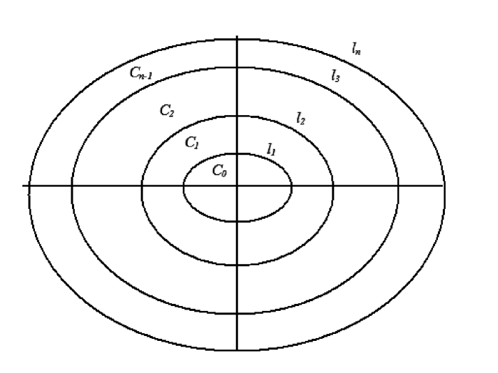
Figure 1: The Gribov horizons

Let us look thus at the eigenvalues equation for the Faddeev-Popov operator $\mathcal{M}^{ab}$, i.e.

$$\mathcal{M}^{ab}\psi^{b}=\epsilon(A)\psi^{a}\;.$$ (79)

For small values of the gauge fields $(A_{\mu},A_{\mu}^{a})$, eq.$\left(\ref{eig}\right)$ is solvable for positive $\epsilon(A)$ only. More precisely, denoting by $\epsilon_{1}(A),\epsilon_{2}(A),\epsilon_{3}(A),....,$ the eigenvalues corresponding to a given field configuration $(A_{\mu},A_{\mu}^{a})$, one has that, for small $(A_{\mu},A_{\mu}^{a})$, all $\epsilon_{i}(A)$ are positive, $\epsilon_{i}(A)>0$, corresponding to field configurations for which $-D_{\mu}^{ac}D_{\mu}^{cb}>g^{2}\varepsilon^{ac}\varepsilon^{bd}A_{\mu}^{c}A_{\mu}^{d}$. However, for a sufficiently large value of the fields $(A_{\mu},A_{\mu}^{a})$, one of the eigenvalues, say $\epsilon_{1}(A)$, turns out to vanish, becoming negative as the fields increase further. This means that the fields $(A_{\mu},A_{\mu}^{a})$ are large enough to ensure the existence of negative energy solutions, i.e. bound states. For a greater magnitude of $(A_{\mu},A_{\mu}^{a})$, a second eigenvalue, say $\epsilon_{2}(A)$, will vanish, becoming negative as the fields increase again. Following Gribov [26], we may thus divide the functional space of the fields into regions $\mathcal{C}_{0},\mathcal{C}_{1},\mathcal{C}_{2},...,\mathcal{C}_{n}$ over which the operator $\mathcal{M}^{ab}$ has $0,1,2,....,n$ negative eigenvalues. These regions are separated by lines $l_{1},l_{2},l_{3},...,l_{n}$ on which the operator $\mathcal{M}^{ab}$ has zero energy solutions. The meaning of Fig.1 is as follows. In the region $\mathcal{C}_{0}$ all eigenvalues of the operator $\mathcal{M}^{ab}$ are positive, i.e. $\mathcal{M}^{ab}>0$. At the boundary $l_{1}$ of the region $\mathcal{C}_{0}$ the first vanishing eigenvalue appears, namely on $l_{1}$ the operator $\mathcal{M}^{ab}$ possesses a normalizable zero mode. In the region $\mathcal{C}_{1}$ the operator $\mathcal{M}^{ab}$ has one bound state,  i.e. one negative energy solution. At the boundary $l_{2}$, a zero eigenvalue reappears. In the region $\mathcal{C}_{2}$ the operator $\mathcal{M}^{ab}$ has two bound states, i.e. two negative energy solutions. On $l_{3}$ a zero eigenvalue shows up again, and so on. The boundaries $l_{1},\;l_{2},\;l_{3},\;....,\;l_{n}$,  on which the operator $\mathcal{M}^{ab}$ has zero eigenvalues are called Gribov horizons. In particular, the boundary $l_{1}$ where the first vanishing eigenvalue appears is called the first horizon. See [28] for an explicit example of a horizon configuration.

It is useful to emphasize that in the region $\mathcal{C}_{0}$, the operator $\mathcal{M}^{ab}$ has only positive eigenvalues. Therefore, this region can be defined as the set of all gauge fields $(A_{\mu},A_{\mu}^{a})$ fulfilling the gauge conditions eqs.(13), (15), for which the Faddeev-Popov operator $\mathcal{M}^{ab}$ is positive definite, see eq.(24). Note also that field configurations belonging to $\mathcal{C}_{0}$ correspond to relative minima of the auxiliary functional $\mathcal{R}[A]$. This follows by observing that the Faddeev-Popov operator $\mathcal{M}^{ab}$ can be obtained by taking the second variation of $\mathcal{R}[A]$ [28].

Let us proceed with the generalization to the maximal Abelian gauge of Gribov’s result stating that for any field close to a horizon there is an equivalent field, i.e. a gauge copy, located on the other side of the horizon, close to the same horizon, see Fig.2

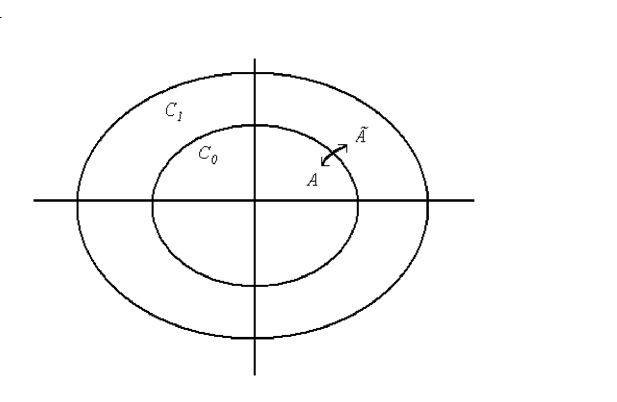
Figure 2: The equivalent fields

Let us start by considering a field configuration $\left(C_{\mu},\;C_{\mu}^{a}\right)$ located on the first Gribov horizon $l_{1}$, namely

$$\mathcal{M}^{ab}\left(C\right)\varphi_{0}^{b} = -\left(D_{\mu}^{ac}(C)D_{\mu}^{cb}(C)+g^{2}\varepsilon^{ac}\varepsilon^{bd}C_{\mu}^{c}C_{\mu}^{d}\right)\varphi_{0}^{b}=0\;,$$

$$D_{\mu}^{ab}\left(C_{\mu}\right)C_{\mu}^{b} = 0\;,$$

$$\partial_{\mu}C_{\mu} = 0\;,$$ (80)

where $\varphi_{0}^{a}$ denotes a normalizable zero mode. In the following it turns out to be useful to introduce the diagonal component $\varphi_{0}$ which, according to eq.(21), is defined as

$$\varphi_{0}=-g\epsilon^{ab}\frac{\partial_{\mu}}{\partial^{2}}\left(C_{\mu}^{a}\varphi_{0}^{b}\right)\;.$$ (81)

Let thus $\left(A_{\mu},A_{\mu}^{a}\right)$ be a field configuration located in the Gribov region $\mathcal{C}_{0}$, close to the horizon $l_{1}$, Fig.2. Following [26] we write

$$A_{\mu}^{a} = C_{\mu}^{a}+a_{\mu}^{a}\;,$$

$$A_{\mu} = C_{\mu}+a_{\mu}\;,$$ (82)

where $\left(a_{\mu},\;a_{\mu}^{a}\right)$ have to be considered as small perturbations. The fields $(A_{\mu},A_{\mu}^{a})$ obey the gauge conditions (13) and (15) which, neglecting higher order terms in the small components $\left(a_{\mu},\;a_{\mu}^{a}\right)$, read

$$D_{\mu}^{ab}(C)a_{\mu}^{b}-g\varepsilon^{ab}C_{\mu}^{b}a_{\mu} = 0\;,$$

$$\partial_{\mu}a_{\mu} = 0\;.$$

The evaluation of the energy eigenvalue $\epsilon(A)$ of the Faddeev-Popov operator $\mathcal{M}^{ab}(A)$ corresponding to the field configuration $\left(A_{\mu},A_{\mu}^{a}\right)$ can be easily handled by means of perturbation theory, yielding

$$\epsilon(A)=\frac{\int d^{4}x\;\varphi_{0}^{a}\left(2g\varepsilon^{ac}a_{\mu}D_{\mu}^{cb}(C)\varphi_{0}^{b}+g^{2}\varepsilon^{ac}\varepsilon^{db}(C_{\mu}^{c}a_{\mu}^{d}+C_{\mu}^{d}a_{\mu}^{c})\varphi_{0}^{b}\right)}{\int d^{4}x\;\varphi_{0}^{a}\varphi_{0}^{a}}\;,$$ (83)

Proceeding as in [26], we introduce the fields

$$\tilde{A}_{\mu}^{a} = C_{\mu}^{a}+\tilde{a}_{\mu}^{a}\;,$$

$$\tilde{A}_{\mu} = C_{\mu}+\tilde{a}_{\mu}\;,$$ (84)

where

$$\tilde{a}_{\mu}^{a} = a_{\mu}^{a}-D_{\mu}^{ab}(C)\varphi_{0}^{b}-g\varepsilon^{ab}C_{\mu}^{b}\varphi_{0}\;,$$

$$\tilde{a}_{\mu} = a_{\mu}-\partial_{\mu}\varphi_{0}-g\varepsilon^{ab}C_{\mu}^{a}\varphi_{0}^{b}\;,$$ (85)

have to be considered as small as compared to $(C_{\mu},C_{\mu}^{a})$. It is not difficult to verify that, to first order in the small components $\left(\tilde{a}_{\mu}^{a},\tilde{a}_{\mu}\right)$, the fields $(\tilde{A}_{\mu},\tilde{A}_{\mu}^{a})$ obey the same gauge conditions of $(A_{\mu},A_{\mu}^{a})$, namely

$$D_{\mu}^{ab}(\tilde{A})\tilde{A}_{\mu}^{b} = 0\;,$$

$$\partial_{\mu}\tilde{A}_{\mu} = 0\;.$$ (86)

The fields $(\tilde{A}_{\mu},\tilde{A}_{\mu}^{a})$ might thus be identified with a Gribov copy of $(A_{\mu},A_{\mu}^{a})$, provided one is able to find a gauge transformation $S$ such that

$$\widetilde{\mathcal{A}}_{\mu} = S^{\dagger}\mathcal{{A}_{\mu}}S+S^{\dagger}\partial_{\mu}S\;,$$

$$\widetilde{\mathcal{A}}_{\mu} = \tilde{A_{\mu}^{a}}T^{a}+\tilde{A_{\mu}}T^{3}\;,$$

$$\mathcal{A}_{\mu} = A_{\mu}^{a}T^{a}+A_{\mu}T^{3}\;.$$ (87)

We shall look at $S$ close to unit, in the form

$$S = 1-\overline{\alpha}+\frac{\overline{\alpha}^{2}}{2}+O(\overline{\alpha}^{3})\;,$$

$$\overline{\alpha} = \alpha^{a}T^{a}+\alpha T^{3}\;,$$ (88)

from which we obtain

$$\tilde{A}_{\mu}^{a} = A_{\mu}^{a}-\left(D_{\mu}^{ab}\alpha^{b}+g\varepsilon^{ab}A_{\mu}^{b}\alpha\right)-\frac{g}{2}\varepsilon^{ab}\alpha^{b}\left(\partial_{\mu}\alpha+g\varepsilon^{cd}A_{\mu}^{c}\alpha^{d}\right)+\frac{g}{2}\varepsilon^{ab}\alpha{D}_{\mu}^{bc}\alpha^{c}-\frac{g^{2}}{2}A_{\mu}^{a}\alpha^{2}\;,$$

$$\tilde{A}_{\mu} = A_{\mu}-\left(\partial_{\mu}\alpha+g\varepsilon^{ab}A_{\mu}^{a}\alpha^{b}\right)-\frac{g}{2}\varepsilon^{ab}\alpha^{a}D_{\mu}^{bc}\alpha^{c}+\frac{g^{2}}{2}A_{\mu}^{a}\alpha^{a}\alpha\;.$$

Furthermore, from eq.(86), it follows

$$\mathcal{M}^{ab}(A)\alpha^{b}+D_{\mu}^{ab}(A)\left[-\frac{g}{2}\varepsilon^{bc}\alpha^{c}\left(\partial_{\mu}\alpha+g\varepsilon^{de}A_{\mu}^{d}\alpha^{e}\right)+\frac{g}{2}\varepsilon^{bc}\alpha{D}_{\mu}^{cd}\alpha^{d}-\frac{g^{2}}{2}A_{\mu}^{b}\alpha^{2}\right]$$

$$-g\varepsilon^{ab}\left(\partial_{\mu}\alpha+g\varepsilon^{cd}A_{\mu}^{c}\alpha^{d}\right)\left(D_{\mu}^{be}\alpha^{e}+g\varepsilon^{be}A_{\mu}^{e}\alpha\right)+g\varepsilon^{ab}A_{\mu}^{b}\left(\frac{g}{2}\varepsilon^{cd}\alpha^{c}D_{\mu}^{de}\alpha^{e}-\frac{g^{2}}{2}A_{\mu}^{c}\alpha^{c}\alpha\right) = 0\;,$$

$$\partial_{\mu}\left[-\left(\partial_{\mu}\alpha+g\varepsilon^{ab}A_{\mu}^{a}\alpha^{b}\right)-\frac{g}{2}\varepsilon^{ab}\alpha^{a}D_{\mu}^{bc}\alpha^{c}+\frac{g^{2}}{2}A_{\mu}^{a}\alpha^{a}\alpha\right] = 0\;.$$

In order to express $\left(\alpha,\alpha^{a}\right)$ in terms of $\left(\varphi_{0},\varphi_{0}^{a}\right)$, we follow [26], and set

$$\alpha^{a} = \varphi_{0}^{a}+\tilde{\varphi}^{a}\;,$$

$$\alpha = \varphi_{0}+\tilde{\varphi}\;,$$ (91)

with $\left(\tilde{\varphi},\tilde{\varphi}^{a}\right)\;$small with respect to $\left(\varphi_{0},\varphi_{0}^{a}\right)$. Condition (LABEL:2ordemcopias1) gives thus

$$\mathcal{M}^{ab}(C)\tilde{\varphi}^{b} = -g\varepsilon^{cb}D_{\mu}^{ac}(C)(a_{\mu}\varphi_{0}^{b})-g\varepsilon^{ac}a_{\mu}D_{\mu}^{cb}(C)\varphi_{0}^{b}-g^{2}\varepsilon^{ac}\varepsilon^{db}(C_{\mu}^{c}a_{\mu}^{d}+C_{\mu}^{d}a_{\mu}^{c})\varphi_{0}^{b}$$

$$+ D_{\mu}^{ab}(C)\left[\frac{g}{2}\varepsilon^{bc}\varphi_{0}^{c}(\partial_{\mu}\varphi_{0}+g\varepsilon^{de}C_{\mu}^{d}\varphi_{0}^{e})-\frac{g}{2}\varepsilon^{bc}\varphi_{0}D_{\mu}^{cd}(C)\varphi_{0}^{d}+\frac{g^{2}}{2}C_{\mu}^{b}\varphi_{0}^{2}\right]$$

$$+ g\varepsilon^{ab}(\partial_{\mu}\varphi_{0}+g\varepsilon^{cd}C_{\mu}^{c}\varphi_{0}^{d})\left[D_{\mu}^{be}(C)\varphi_{0}^{e}+g\varepsilon^{be}C_{\mu}^{e}\varphi_{0}\right]$$

$$- g\varepsilon^{ab}C_{\mu}^{b}\left[\frac{g}{2}\varepsilon^{cd}\varphi_{0}^{c}D_{\mu}^{de}(C)\varphi_{0}^{e}-\frac{g^{2}}{2}C_{\mu}^{c}\varphi_{0}^{c}\varphi_{0}\right]\;.$$

Note that eq.(LABEL:2ordemcopias2) can be cast in the form

$$\partial^{2}\tilde{\varphi}^{a}=\mathcal{P}^{a}(C,a,\varphi_{0})+\mathcal{Q}^{ab}(C,\varphi_{0})\tilde{\varphi}^{b}\;,$$ (93)

where $\mathcal{P}^{a}$ and $\mathcal{Q}^{ab}$ are independent from $\tilde{\varphi}$, i.e.

$$\mathcal{-P}^{a}(C,a,\varphi_{0}) = -g\varepsilon^{cb}D_{\mu}^{ac}(C)(a_{\mu}\varphi_{0}^{b})-g\varepsilon^{ac}a_{\mu}D_{\mu}^{cb}(C)\varphi_{0}^{b}-g^{2}\varepsilon^{ac}\varepsilon^{db}(C_{\mu}^{c}a_{\mu}^{d}+C_{\mu}^{d}a_{\mu}^{c})\varphi_{0}^{b}$$

$$+ D_{\mu}^{ab}(C)\left[\frac{g}{2}\varepsilon^{bc}\varphi_{0}^{c}(\partial_{\mu}\varphi_{0}+g\varepsilon^{de}C_{\mu}^{d}\varphi_{0}^{e})-\frac{g}{2}\varepsilon^{bc}\varphi_{0}D_{\mu}^{cd}(C)\varphi_{0}^{d}+\frac{g^{2}}{2}C_{\mu}^{b}\varphi_{0}^{2}\right]$$

$$+ g\varepsilon^{ab}(\partial_{\mu}\varphi_{0}+g\varepsilon^{cd}C_{\mu}^{c}\varphi_{0}^{d})\left[D_{\mu}^{be}(C)\varphi_{0}^{e}+g\varepsilon^{be}C_{\mu}^{e}\varphi_{0}\right]$$

$$- g\varepsilon^{ab}C_{\mu}^{b}\left[\frac{g}{2}\varepsilon^{cd}\varphi_{0}^{c}D_{\mu}^{de}(C)\varphi_{0}^{e}-\frac{g^{2}}{2}C_{\mu}^{c}\varphi_{0}^{c}\varphi_{0}\right]\;,$$

and

$$\mathcal{Q}^{ab}(C,\varphi_{0})=2g\varepsilon^{ab}C_{\mu}\partial_{\mu}-g^{2}\varepsilon^{ac}\varepsilon^{cb}C_{\mu}C_{\mu}-g^{2}\varepsilon^{ac}\varepsilon^{bd}C_{\mu}^{c}C_{\mu}^{d}\;.$$ (95)

Equation (93) can be solved recursively for $\tilde{\varphi}^{a}$, namely

$$\tilde{\varphi}^{a}=\frac{1}{\partial^{2}}\mathcal{P}^{a}+\frac{1}{\partial^{2}}\mathcal{Q}^{ab}\frac{1}{\partial^{2}}\mathcal{P}^{b}+......\;$$ (96)

This allows us to obtain a recursive expression for the parameters $\left(\alpha,\alpha^{a}\right)$ of eq.(91), an thus for the gauge transforamtion $S$ we are looking for, eq.(88).

Moreover, recalling that

$$\mathcal{M}^{ab}\left(C\right)\varphi_{0}^{b}=0\;,$$ (97)

one finds

$$\int d^{4}x\;\varphi_{0}^{a}\mathcal{M}^{ab}(C)\tilde{\varphi}^{b}\;=0\;,$$ (98)

so that

$$0 = \int d^{4}x\;\varphi_{0}^{a}\;\left[-2g\varepsilon^{ac}a_{\mu}D_{\mu}^{cb}(C)\varphi_{0}^{b}-g^{2}\varepsilon^{ac}\varepsilon^{db}(C_{\mu}^{c}a_{\mu}^{d}+C_{\mu}^{d}a_{\mu}^{c})\varphi_{0}^{b}\right.$$ (99)

$$\;\;\left.\;+g\varepsilon^{ab}(\partial_{\mu}\varphi_{0})D_{\mu}^{bc}(C)\varphi_{0}^{c}-2g^{2}\varepsilon^{ab}\varepsilon^{cd}C_{\mu}^{b}\varphi_{0}^{c}D_{\mu}^{de}(C)\varphi_{0}^{e}+g^{3}\varepsilon^{ab}C_{\mu}^{b}C_{\mu}^{c}\varphi_{0}^{c}\varphi_{0}\right]\;.$$

Let us now check on which side of the horizon $l_{1}$ the equivalent fields $(\tilde{A}_{\mu},\tilde{A}_{\mu}^{a})$ are located. As done before, we look at the energy eigenvalue $\epsilon(\tilde{A})$, given by

$$\epsilon(\tilde{A})=\frac{\int d^{4}x\;\varphi_{0}^{a}\left(2g\varepsilon^{ac}\tilde{a}_{\mu}D_{\mu}^{cb}(C)\varphi_{0}^{b}+g^{2}\varepsilon^{ac}\varepsilon^{db}(C_{\mu}^{c}\tilde{a}_{\mu}^{d}+C_{\mu}^{d}\tilde{a}_{\mu}^{c})\varphi_{0}^{b}\right)}{\int d^{4}x\;\varphi_{0}^{a}\varphi_{0}^{a}}\;.$$ (100)

Finally, form eqs.(85), (99) it follows that

$$\epsilon(\tilde{A})=-\epsilon(A)\;.$$ (101)

Thus, if the configuration $(A_{\mu},A_{\mu}^{a})$, close to $l_{1}$, is located in the region $\mathcal{C}_{0}$, $\epsilon(A)>0$, there is an equivalent field configuration $(\tilde{A}_{\mu},\tilde{A}_{\mu}^{a})$, eqs.(84), (85), close to $l_{1}$, which is located in $\mathcal{C}_{1}$, $\epsilon(\tilde{A})=-\epsilon(A)<0$. This derivation, which can be repeated to fields close to any horizon $l_{n}$, generalizes Gribov’s statement to the case of the maximal Abelian gauge .

Appendix B Faddeev-Popov quantization of Yang-Mills theory in the maximal Abelian gauge

We provide here a detailed summary of the Faddeev-Popov quantization of Yang-Mills theory in the maximal Abelian gauge. Following [13], let us start by giving the $BRST$ transformations of all fields, namely

$$sA_{\mu}^{a} = -\left(D_{\mu}^{ab}c^{b}+g\varepsilon^{\,ab}A_{\mu}^{b}c\right)\;,$$

$$sA_{\mu} = -\left(\partial_{\mu}c+g\varepsilon^{ab}A_{\mu}^{a}c^{b}\right)\;,$$

$$sc^{a} = g\varepsilon\,^{ab}c^{b}c\;,$$

$$\,sc = \frac{g}{2}\,\varepsilon\,^{ab}c^{a}c^{b},$$

$$s\overline{c}^{a} = b^{a}\;,$$

$$s\overline{c} = b\;,$$

$$sb^{a} = 0\;,$$

$$\,sb = 0\;,$$ (102)

with

$$s^{2}=0\;,$$ (103)

where $\left(\overline{c}^{a},c^{a}\right)$ and $\left(\overline{c},c\right)$ are the off-diagonal and diagonal Faddeev-Popov ghosts, while $\left(b^{a},b\right)\;$denote the Lagrange multipliers. For the gauge-fixed Yang-Mills theory one has

$$S_{\mathrm{YM}}+S_{\mathrm{MAG}}+S_{\mathrm{diag}}\;,$$ (104)

$$s\left(S_{\mathrm{YM}}+S_{\mathrm{MAG}}+S_{\mathrm{diag}}\right)=0\;,$$ (105)

where

$$S_{\mathrm{YM}}=\frac{1}{4}\int d^{4}x\,\left(F_{\mu\nu}^{a}F_{\mu\nu}^{a}+F_{\mu\nu}F_{\mu\nu}\right)\;,$$ (106)

and $S_{\mathrm{MAG}},$ $S_{\mathrm{diag}}$ being the gauge fixing terms corresponding to the off-diagonal and diagonal sectors, respectively. They are given by

$$S_{\mathrm{MAG}} = s\,\int d^{4}x\,\left(\overline{c}^{a}\left(D_{\mu}^{ab}A_{\mu}^{b}+\frac{\alpha}{2}b^{a}\right)-\frac{\alpha}{2}g\varepsilon\,^{ab}\overline{c}^{a}\overline{c}^{b}c\right)\;$$ (107)

$$= \int d^{4}x\left(b^{a}\left(D_{\mu}^{ab}A_{\mu}^{b}+\frac{\alpha}{2}b^{a}\right)+\overline{c}^{a}D_{\mu}^{ab}D_{\mu}^{bc}c^{c}+g\overline{c}^{a}\varepsilon^{ab}\left(D_{\mu}^{bc}A_{\mu}^{c}\right)c\right.$$

$$\left.-\alpha g\varepsilon^{ab}b^{a}\overline{c}^{b}c-g^{2}\varepsilon^{ab}\varepsilon^{cd}\overline{c}^{a}c^{d}A_{\mu}^{b}A_{\mu}^{c}-\frac{\alpha}{4}g^{2}\varepsilon^{ab}\varepsilon^{cd}\overline{c}^{a}\overline{c}^{b}c^{c}c^{d}\right)\;,$$

and

$$S_{\mathrm{diag}}=s\,\int d^{4}x\,\;\overline{c}\partial_{\mu}A_{\mu}\;=\int d^{4}x\,\;\left(b\partial_{\mu}A_{\mu}+\overline{c}\partial_{\mu}\left(\partial_{\mu}c+g\varepsilon^{ab}A_{\mu}^{a}c^{b}\right)\right)\;.$$ (108)

Note that, for renormalizability purposes, a gauge parameter $\alpha$ has to be introduced in the off-diagonal part of the gauge fixing, eq.$\left(\ref{smm}\right)$. The maximal Abelian gauge condition, $D_{\mu}^{ab}A_{\mu}^{b}=0$, is recovered in the limit $\alpha\rightarrow$ $0$, which has to be taken after the removal of the ultraviolet divergences [13]. In fact, some of the terms proportional to $\alpha$ would reappear due to radiative corrections, even if $\alpha=0$. See, for example, [25]. Moreover, the action $\left(\ref{smag}\right)$ is multiplicatively renormalizable to all orders of perturbation theory [12, 13].

Therefore, for the partition function expressing the Faddeev-Popov quantization of Yang-Mills theory in the maximal Abelian gauge we have

$$\mathcal{Z}=\int DA_{\mu}DA_{\mu}^{a}Db^{a}DbDc^{a}DcD\overline{c}^{a}D\overline{c}\;e^{-\left(S_{\mathrm{YM}}+S_{\mathrm{MAG}}+S_{\mathrm{diag}}\right)\;}.$$ (109)

Taking the limit $\alpha\rightarrow$ $0$ and integrating over the Lagrange multipliers $\left(b^{a},b\right)$, one gets

$$\mathcal{Z} = \int DA_{\mu}DA_{\mu}^{a}Dc^{a}DcD\overline{c}^{a}D\overline{c}\;\delta\left(D_{\mu}^{ab}A_{\mu}^{b}\right)\delta\left(\partial_{\mu}A_{\mu}\right)e^{-S_{\mathrm{YM}}\;}$$

$$\;\;\;\;\;\;\times\exp\left(-\int d^{4}x\left(\,\left(\overline{c}^{a}D_{\mu}^{ab}D_{\mu}^{bc}c^{c}-g^{2}\varepsilon^{ab}\varepsilon^{cd}\overline{c}^{a}c^{d}A_{\mu}^{b}A_{\mu}^{c}\right)+\overline{c}\partial_{\mu}\left(\partial_{\mu}c+g\varepsilon^{ab}A_{\mu}^{a}c^{b}\right)\right)\right)\;.$$

To deal with the diagonal ghosts $(\overline{c},c)$ we perform now the change of variables

$$c \rightarrow \widetilde{c}=c+g\frac{\partial_{\mu}}{\partial^{2}}\left(\varepsilon^{ab}A_{\mu}^{a}c^{b}\right)\;,$$

$$c^{a} \rightarrow c^{a}\;,$$

$$A_{\mu}^{a} \rightarrow A_{\mu}^{a}\;,$$ (111)

all other fields remaining unchanged. It is easy to check that

$$\partial_{\mu}\left(\partial_{\mu}c+g\varepsilon^{ab}A_{\mu}^{a}c^{b}\right)\rightarrow\partial^{2}\widetilde{c}\;,$$ (112)

and that the Jacobian $J$ corresponding to $\left(\text{\ref{chv}}\right)$ is field independent. In fact

$$J=\det\left(\;\begin{tabular}[]{lll}$1$&$g\varepsilon^{ac}\frac{\partial_{\mu}}{\partial^{2}}c^{c}$&$g\varepsilon^{cd}\frac{\partial_{\mu}}{\partial^{2}}A_{\mu}^{c}$\\ $0$&$\delta^{ab}\delta_{\mu\nu}$&$0$\\ $0$&$0$&$\delta^{bd}$\end{tabular}\right)=\mathrm{const}.\;\;$$ (113)

One sees thus that the transformation $\left(\text{\ref{chv}}\right)$ allows us to decouple the diagonal ghosts from the theory, namely

$$\mathcal{Z} = \int DA_{\mu}DA_{\mu}^{a}Dc^{a}D\widetilde{c}D\overline{c}^{a}D\overline{c}\;\delta\left(D_{\mu}^{ab}A_{\mu}^{b}\right)\delta\left(\partial_{\mu}A_{\mu}\right)e^{-S_{\mathrm{YM}}\;}$$ (114)

$$\;\;\;\;\;\;\times\exp\left(-\int d^{4}x\left(\,\left(\overline{c}^{a}D_{\mu}^{ab}D_{\mu}^{bc}c^{c}-g^{2}\varepsilon^{ab}\varepsilon^{cd}\overline{c}^{a}c^{d}A_{\mu}^{b}A_{\mu}^{c}\right)+\overline{c}\partial^{2}\widetilde{c}\right)\right)\;,$$

so that they can be integrated out, yielding

$$\mathcal{Z} = \mathcal{N}\int DA_{\mu}DA_{\mu}^{a}Dc^{a}D\overline{c}^{a}\;\delta\left(D_{\mu}^{ab}A_{\mu}^{b}\right)\delta\left(\partial_{\mu}A_{\mu}\right)e^{-S_{\mathrm{YM}}\;}$$ (115)

$$\;\;\;\;\;\;\times\exp\left(-\int d^{4}x\left(\,\left(\overline{c}^{a}D_{\mu}^{ab}D_{\mu}^{bc}c^{c}-g^{2}\varepsilon^{ab}\varepsilon^{cd}\overline{c}^{a}c^{d}A_{\mu}^{b}A_{\mu}^{c}\right)\right)\right)\;,$$

where $\mathcal{N}$ is an irrelevant constant factor. It is worth remarking that the change of variables $\left(\text{\ref{chv}}\right)$ seems to be a peculiar feature of the maximal Abelian gauge. One could try in fact to perform such a kind of transformation to decouple the Faddeev-Popov ghosts in other cases as, for instance, the Landau gauge. However, it is straightforward to check now that the Jacobian of the decoupling transformation is no more field independent. It gives back precisely the Faddeev-Popov determinant for the Landau gauge, so that the Faddeev-Popov ghosts show up again.

Finally, integrating over the off-diagonal ghosts $\left(\overline{c}^{a},c^{a}\right)$, it follows

$$\mathcal{Z}=\mathcal{N}\int DA_{\mu}DA_{\mu}^{a}\;\delta\left(D_{\mu}^{ab}A_{\mu}^{b}\right)\delta\left(\partial_{\mu}A_{\mu}\right)\left(\det\left(\mathcal{M}^{ab}\right)\right)e^{-S_{\mathrm{YM}}\;}\;,$$ (116)

where $\mathcal{M}^{ab}$ is the off-diagonal Faddeev-Popov operator, as given in eq.$\left(\text{\ref{offop}}\right)$. Expression $\left(\text{\ref{pftf}}\right)$ will be taken as the starting point for the implementation of the restriction to the Gribov region $\mathcal{C}_{0}$ for the maximal Abelian gauge.