D-Brane Propagation in Two-Dimensional Black Hole Geometries

Abstract:

We study propagation of D0-brane in two-dimensional Lorentzian black hole backgrounds by the method of boundary conformal field theory of $SL(2,\mathbb{R})/U(1)$ supercoset at level $k$. Typically, such backgrounds arise as near-horizon geometries of $k$ coincident non-extremal NS5-branes, where $1/k$ measures curvature of the backgrounds in string unit and hence size of string worldsheet effects. At classical level, string worldsheet effects are suppressed and D0-brane propagation in the Lorentzian black hole geometry is simply given by the Wick rotation of D1-brane contour in the Euclidean black hole geometry. Taking account of string worldsheet effects, boundary state of the Lorentzian D0-brane is formally constructible via Wick rotation from that of the Euclidean D1-brane. However, the construction is subject to ambiguities in boundary conditions. We propose exact boundary states describing the D0-brane, and clarify physical interpretations of various boundary states constructed from different boundary conditions. As it falls into the black hole, the D0-brane radiates off to the horizon and to the infinity. From the boundary states constructed, we compute physical observables of such radiative process. We find that part of the radiation to infinity is in effective thermal distribution at the Hawking temperature. We also find that part of the radiation to horizon is in the Hagedorn distribution, dominated by massive, highly non-relativistic closed string states, much like the tachyon matter. Remarkably, such distribution emerges only after string worldsheet effects are taken exactly into account. From these results, we observe that nature of the radiation distribution changes dramatically across the conifold geometry $k=1$ ($k=3$ for the bosonic case), exposing the ‘string - black hole transition’ therein.

1 Introduction and Summary

An important yet unsolved problem in string theory is an ab initio formulation of dynamics in time-dependent closed string background. Cosmological or black hole backgrounds are outstanding situations of this sort. In these situations, because there is no globally definable timelike Killing vector, there always arise Bogoliubov excitation of the vacuum, leading to cosmological particle production and Hawking radiation. At present, however, full-fledged string theoretic description of the these processes is unavailable. Open string counterpart turned out more manageable. Decay of unstable D-brane, described by open string tachyon rolling [1], is amenable to exact conformal field theory approach, thus studied extensively in recent years. Still, some issues are left out unsettled, especially, ambiguity in prescribing timelike conformal field theories and the open string vacuum thereof.

One may hope to find the situation better for the well-known two-dimensional black hole, which admits exact conformal field theory description [2], and to understand physics inside the horizon and the spacelike singularity. For such purposes, we have learned through a variety of other situations that D-brane serves as a better probe than closed string. Our goal is to investigate dynamics of D0-brane propagating in the two-dimensional black hole geometries. In this paper, we shall take the first step toward the goal: understanding D0-brane dynamics in the causal region outside the horizon, with particular focus on large curvature regime, where the string worldsheet effects become strong. The D0-brane serves as a local probe of the black hole geometries and, in a certain sense, may be considered as an analog of ZZ-brane in the Liouville theory.

The two-dimensional black hole is often considered as a toy model of more realistic higher-dimensional black holes. This is not necessarily so, since the background is intimately related to the black NS5-branes, whose background [4] is given by

$$\mbox{d}s^{2}=-\left(1-\frac{r_{0}^{2}}{r^{2}}\right)\mbox{d}t^{2}+\left(1+\frac{k\alpha^{\prime}}{r^{2}}\right)\left(\frac{\mbox{d}r^{2}}{1-\frac{r_{0}^{2}}{r^{2}}}+r^{2}\mbox{d}\Omega_{3}^{2}\right)+\mbox{d}{\bf y}^{2}_{\mathbb{R}^{5}}~{},~{}~{}~{}e^{2\Phi(r)}=g_{s}^{2}\left(1+\frac{k\alpha^{\prime}}{r^{2}}\right)$$ (1)

along with $k$-units of NS-NS $H_{3}$-flux penetrating through $\mathbb{S}^{3}$. Thus, $k$ refers to the number of NS5-branes at $r=0$, $r=r_{0}$ is the location of the event horizon, ${\bf y}$ are the spatial coordinates of the planar NS5-brane worldvolume, and $g_{s}$ is the string coupling constant at infinity. Since the NS5-brane is black, it breaks space-time supersymmetries completely and Hawking radiates.

One hopes to gain intuition by studying classical D0-brane dynamics near the horizon. So, consider taking various near-horizon limits of the black NS5-brane (1). One type of near-horizon limit is $r_{0}\rightarrow 0$ and $g_{s}\rightarrow 0$ independently, leading to the ‘throat geometry’ of extremal NS5-branes [5, 6]:

$$\mbox{d}s^{2}=-\mbox{d}t^{2}+k\alpha^{\prime}\mbox{d}\rho^{2}+k\alpha^{\prime}\mbox{d}\Omega_{3}^{2}+\mbox{d}{\bf y}_{\mathbb{R}^{5}}^{2}~{},\qquad{\Phi}=-\rho+\text{constant}\ ,$$ (2)

where $r=\sqrt{k\alpha^{\prime}}\exp\rho$. This background is describable by the exact conformal field theory involving linear dilaton and $SU(2)_{k}$ super Wess-Zumino-Witten (WZW) model:

$$\Big{[}\mathbb{R}_{t}\times\mathbb{R}_{\rho,\sqrt{2\over k}}\times SU(2)_{k}\Big{]}_{\perp}\times\Big{[}\mathbb{R}^{5}\Big{]}_{||}.$$

The first part describes the five-dimensional curved spacetime transverse to the NS5-brane, while the second part describes the flat spatial directions parallel to NS5-brane. The criticality condition is satisfied for any k because

$$\left(1+\frac{6}{k}+\frac{1}{2}\right)+3\times\left(\frac{k-2}{k}+\frac{1}{2}\right)+6\times\left(1+\frac{1}{2}\right)=15$$ (3)

D-brane dynamics in this background was studied in [7, 8] via the Dirac-Born-Infeld (DBI) approach, and observed that it strikingly resembles the rolling tachyon of unstable D-brane in ambient flat spacetime [1, 9, 10]. This map, which we refer as ‘radion-tachyon correspondence’, offers a useful guide for understanding D-brane propagating in curved spacetime geometry in terms of known results regarding rolling tachyon dynamics. Introducing ‘tachyon’ variable $X=\rho$, DBI Lagrangian of the D0-brane propagating in the background (2) is recastable to that of rolling tachyon:

$$L_{\rm D0}=-e^{-\Phi}\sqrt{\left({\mbox{d}s\over\mbox{d}t}\right)^{2}}=-V(X)\sqrt{1-\dot{X}^{2}}\qquad\mbox{where}\qquad V(X)=M_{0}\,e^{X}.$$ (4)

The energy is conserved, so solving $V(X)/\sqrt{1-\dot{X}^{2}}=1$, we obtain D0-brane’s geodesic as

$$e^{X}={e^{\rho_{o}}\over\cosh(t-t_{o})}\qquad\mbox{viz.}\qquad e^{\rho}\cosh(t-t_{o})=e^{\rho_{o}}.$$ (5)

This is the Lorentzian counterpart of so-called ‘hairpin’ profile. In the previous works [13, 14], we constructed exact boundary states of the D-brane and analyzed rolling dynamics of the D-brane in detail. A technical difficulty was that the dilaton blows up at the core, hampering further analysis by the strong coupling singularity.

Another type of near-horizon limit is $r_{0}\rightarrow 0$ and $g_{s}\rightarrow 0$ while keeping the energy density above the extremal configuration $\mu\equiv{r_{0}^{2}}/{g_{s}^{2}\alpha^{\prime}}$ fixed. It yields ‘throat geometry’ of the near-extremal NS5-branes (1) [18]:

$$\mbox{d}s^{2}=-\tanh^{2}\rho\,\mbox{d}t^{2}+k\alpha^{\prime}\mbox{d}\rho^{2}+k\alpha^{\prime}\mbox{d}\Omega_{3}^{2}+\mbox{d}{\bf y}_{\mathbb{R}^{5}}^{2}~{},\qquad e^{2\Phi}=\frac{k}{\mu\cosh^{2}\rho}~{},$$ (6)

where $r=r_{0}\cosh\rho$. For $(t,\rho)$-subspace, the metric and the dilaton coincide with those of the two-dimensional black hole. This Lorentzian black hole is describable by Kazama-Suzuki supercoset conformal field theory $SL(2;\mathbb{R})_{k}/U(1)$ (where $U(1)$ subgroup is chosen to be the non-compact component (space-like direction)) of central charge $c=3(1+2/k)$. Likewise, taking account of the NS-NS $H_{3}$-flux penetrating through $\mathbb{S}^{3}$ which is omitted in (6), the angular part $\mathbb{S}^{3}$ is describable by the (super) $SU(2)$-WZW model. In this way, the string background of the nonextremal NS5-brane is reduced to a solvable superconformal field theory system:

$$\Big{[}{SL(2;\mathbb{R})_{k}\over U(1)}\times SU(2)_{k}\Big{]}_{\perp}\times\Big{[}\,\mathbb{R}^{5}\,\Big{]}_{||}~{}.$$ (7)

Here, the first part describes the five-dimensional curved spacetime (including the time direction) transverse to the NS5-brane, while the second part describes the flat spatial directions parallel to the NS5-brane. The criticality condition is satisfied for any $k$ as in (3). Upon Wick rotation, Euclidean black hole has the ‘cigar geometry’, described by the coset conformal field theory $SL(2;\mathbb{R})_{k}/U(1)\simeq{\mathbb{H}}^{3}_{+}/\mathbb{R}$ (where $U(1)$ subgroup is the compact component). Asymptotically, circumference of the cigar geometry is $2\pi\sqrt{\alpha^{\prime}k}$, and is identified with inverse of the Hawking temperature.

Again, by introducing ‘tachyon’ variable $Y\equiv\log\sinh\rho$, DBI Lagrangian of the D0-brane is castable to that of rolling tachyon:

$$L_{\rm D0} = -e^{-\Phi}\sqrt{\left({\mbox{d}s\over\mbox{d}t}\right)^{2}}=-V(Y)\sqrt{1-\dot{Y}^{2}}\qquad\mbox{where}\qquad V(Y)=M_{0}\,e^{Y}~{}.$$ (8)

We now find D0-brane’s geodesic as

$$e^{Y}={\sinh\rho_{o}\over\cosh(t-t_{o})}\qquad\mbox{viz.}\qquad\sinh\rho\cosh(t-t_{o})=\sinh\rho_{o}~{}.$$ (9)

Euclidean counterpart of the geodesic (9) describes D1-brane profile in the Euclidean two-dimensional black hole background. An important point is that, in sharp contrast to the extremal background (2), the dilaton is finite everywhere. Thus, the strong coupling singularity is now capped off by the horizon.

In both cases, it is elementary to understand classical dynamics of the D0-brane: both by gravity and by strong string coupling gradient, D0-brane is pulled in and finds its minimum energy and rest mass at the location of the NS5-brane. This also fits to the observation that the spacetime supersymmetry is completely broken as the NS5-brane and the D0-brane preserve different combinations of the supercharges. Eventually, D0-brane would melt into fluxes of NS5-brane worldvolume gauge field and form a non-threshold bound-state. As the D0-brane is pulled in, acceleration would grow and radiate off the binding energy into closed string modes.

Interestingly, the DBI Lagrangian of D0-brane is identical for both extremal and non-extremal NS5-brane backgrounds, see (4) and (8). Consequently, the geodesics are also identical in $X$ or $Y$ coordinate. Does this imply that the two-dimensional black hole is featureless and not quite black? As we shall explain in much detail, this coincidence turns out simply an artifact of DBI analysis and disappears in full-fledged boundary conformal field theory description for the D0-brane boundary states. It also hints that the radion-tachyon correspondence (based on DBI analysis alone) would break down in non-extremal NS5-brane background, and we will see such indications from exact boundary conformal field theory analysis.

By construction, D-brane boundary states is obtainable from the coupling of the D-brane to closed string modes. Semiclassically, this can be done by overlapping the geodesic (9) to the mini-superspace wave function of the closed string modes. Thus, in section 2, after recapitulating the mini-superspace wave function in the Euclidean black hole background, we shall construct the boundary state of the Euclidean D1-brane [19] by taking the inner product. Being in Euclidean background, the construction is free from ambiguity.

We are primarily interested in D0-brane’s boundary state in Lorentzian background. Formally, the boundary state is obtainable by Wick rotation of that for the Euclidean D1-brane, as constructed in section 2. However, the Wick rotation is not unique and appropriate analytic continuation has to be specified. Causal region of the Lorentzian black hole background has four boundaries: past and future horizons ${\cal H}^{\pm}$, and past and future asymptotic infinities ${\cal I}^{\pm}$. See Figure 1. The specification amounts to imposing boundary conditions at these four null infinities. In section 3, with careful treatment of the boundary conditions, we construct several boundary states of the D0-brane, corresponding to physically motivated boundary conditions: (1) D0-brane emitted from past horizon, (2) D0-brane absorbed to future horizon, and (3) time-symmetric D0-brane. As a useful mnemonic, via the radion-tachyon correspondence (extended to finite temperature background), (1) and (2) are the counterpart of half S-brane, while (3) is the counterpart of full S-brane.

Figure 1: Penrose diagram of the two-dimensional black hole. We focus on the causal region I outside the horizon. Boundaries of the region I consist of past and future asymptotic infinities ${\cal I}^{\pm}$ and past and future horizons ${\cal H}^{\pm}$.

The D0-brane propagating in curved spacetime emits closed string excitations. One expects that in general radiation rate would be proportional to spacetime curvature. In the eternal black hole background, where the future-directed asymptotic infinities consist of ${\cal H}^{+}$ and ${\cal I}^{+}$, the radiation emitted by the D0-brane propagates out to either of them. In section 4, we estimate radiation distribution for incoming part ${\cal N}_{\rm in}(M)$ (as measured at ${\cal H}^{+}$) and outgoing part ${\cal N}_{\rm out}(M)$(as measured at ${\cal I}^{+}$) for a fixed transverse mass $M$. Intuitively, the radiation distribution ought to depend sensitively on the background curvature scale, set by the level $k$. Curiously, we find that the radiation rate depends on the Hawking temperature! This has to do with the novel feature that the Hagedorn and the Hawking temperatures, $T_{\rm Hg}$ and $T_{\rm Hw}$, in the two-dimensional black hole background are both set by $k$:

$$T_{\rm Hg}=\frac{1}{\beta_{\rm Hg}}={1\over 4\pi\sqrt{1-{1\over 2k}}}\qquad\mbox{and}\qquad T_{\rm Hw}=\frac{1}{\beta_{\rm Hw}}=\frac{1}{2\pi\sqrt{2k}}.$$

Especially, the Hawking temperature is independent of the non-extremality $r_{0}$ or $\mu$.

Notice that two temperature scales meet at $k=1$, viz. the conifold geometry, so we anticipate some sort of cross-over or phase transition. For $k>1$, D0-brane energy is emitted almost all to incoming mode toward ${\cal H}^{+}$ and small to outgoing mode toward ${\cal I}^{+}$:

$${{\cal N}_{\rm out}(M)\over{\cal N}_{\rm in}(M)}\sim{e^{-{1\over 2}\beta_{\rm Hw}M}\over e^{-{1\over 2}\beta_{\rm Hg}M}}\ll 1.$$

For $k<1$, only small portion of the D0-brane energy is emitted, equally distributed between the incoming and the outgoing parts:

$${{\cal N}_{\rm out}(M)\over{\cal N}_{\rm in}(M)}\sim 1.$$

The distribution does not appear to be the radiation pattern one would expect in black hole background, where the black hole would absorb most of the radiation (as well as D0-brane). This brings out a question: if $k<1$ background were not associated with black hole, what would it be?

In section 5, we argue that $k=1$ is a critical point of black hole - string phase transition, where the branching ratio between incoming and outgoing part of the radiation provides an ‘order parameter’. Our interpretation fits nicely with recent observation of [21], where the same kind of phase transition was pointed out for $AdS_{3}$ and linear dilaton backgrounds. Given that the NS5-brane background is holographically dual to Little String Theory (LST), it is natural to ask what the holographic dual of the D0-brane falling into the NS5-brane. Adopting the proposal [15] that the dual process is identifiable with decay of a defect or soliton in the LST and taking reasonable assumption concerning $k$-dependence of LST’s decay number distribution and density of states, we show that the defect decay rate as computed within LST fits perfectly with the D0-brane radiation rate as computed in the bulk (viz. black hole background). Interestingly, the two-dimensional black hole at $k=1/2$ belongs not quite to the black hole phase but to the far extreme of the string phase. Long string condensation in two-dimensional string theory was recently studied via non-singlet matrix model [22]. It would be interesting to study D0-brane dynamics in this matrix model and compare with our results.

In section 6, we extend the boundary state analysis to Ramond-Ramond (R-R) sector by spectral flow, and, in section 7, we also analyze the limit the NS5-brane becomes extremal, thus making contact with our earlier results. In section 8, we return to the issue of boundary conditions and propose yet another physically motivated one: the Hartle-Hawking boundary condition. This boundary condition is particularly compelling because a puzzle concerning origin/fate of the conserved R-R charge of the D0-brane gets around, and also fits well with the radiation rate computed in section 4.

2 D1-brane on Euclidean Two-Dimensional Black Hole

In this section, we study boundary state description of the D1-brane profile on the Euclidean two-dimensional black hole geometries. We shall begin with recapitulating aspects of the closed string spectrum relevant for foregoing analysis.

2.1 Mini-superspace analysis of closed strings

Consider the Euclidean two-dimensional black hole background, known as ‘cigar geometry’:

$$\mbox{d}s^{2}\equiv G_{ij}\mbox{d}x^{i}\mbox{d}x^{j}=2k(\mbox{d}\rho^{2}+\tanh^{2}\rho\mbox{d}\theta^{2})\qquad\mbox{and}\qquad e^{\Phi}=\frac{e^{\Phi_{0}}}{\cosh\rho}~{}.$$ (10)

Recall that $k$ sets characteristic curvature radius in unit of the string scale and hence string worldsheet effects, while $e^{\Phi_{0}}$ sets the maximum value of the string coupling at the tip $\rho=0$ of the cigar geometry. We shall assume the limit $k\gg 1$ and $e^{-\Phi_{0}}\gg 1$: this limit suppresses both string worldsheet and spacetime quantum effects and facilitates to truncate closed string spectrum to zero-modes, viz. to mini-superspace approximation.

In the mini-superspace approach, difference between bosonic strings (with no worldsheet supersymmetry) and fermionic strings (with ${\cal N}=2$ worldsheet supersymmetry) becomes unimportant. The closed string Hamiltonian $L_{0}+\overline{L}_{0}$ is reduced in the mini-superspace approximation to the target space Laplacian $\Delta_{0}$, where:

$$\Delta_{0} = \frac{1}{e^{-2\Phi}\sqrt{G}}\partial_{i}\left(e^{-2\Phi}\sqrt{G}G^{ij}\partial_{j}\right)\equiv-\frac{1}{2k}[\partial_{\rho}^{2}+2\coth 2\rho\partial_{\rho}+\coth^{2}\rho\partial_{\theta}^{2}]~{}.$$ (11)

The Hamiltonian is defined with respect to the volume element:

$$\mbox{d}\mbox{Vol}=e^{-2\Phi}\sqrt{G}\mbox{d}\rho\mbox{d}\theta:={2k}\sinh\rho\cosh\rho\mbox{d}\rho\,\mbox{d}\theta\equiv k\sinh 2\rho\mbox{d}\rho\,\mbox{d}\theta~{},$$ (12)

inherited from the Haar measure on the $SL(2;\mathbb{R})$ group manifold. In the volume element, the dilaton factor $e^{-2\Phi}$ is taken into account, as the inner product for closed string states is defined by the worldsheet two-point correlators on the sphere. The normalized eigenfunctions are obtained straightforwardly [3, 19]. They are:

$$\phi_{n}^{j}(\rho,\theta)=-\frac{\Gamma^{2}(-j+\frac{|n|}{2})}{\Gamma(|n|+1)\Gamma(-2j-1)}e^{in\theta}\left[\sinh^{|n|}\rho\cdot F\left(j+1+\frac{|n|}{2},-j+\frac{|n|}{2};|n|+1;-\sinh^{2}\rho\right)\right]~{},$$ (13)

where $F(\alpha,\beta;\gamma;z)$ is the Gaussian hypergeometric function. These eigenfunctions correspond to the primary state vertex operators of conformal weights

$$h=\tilde{h}=-\frac{j(j+1)}{k-2}+\frac{n^{2}}{4k}\qquad\mbox{or}\qquad h=\tilde{h}=-\frac{j(j+1)}{k}+\frac{n^{2}}{4k}$$ (14)

for bosonic and fermionic strings, respectively. We shall focus on the continuous series, parametrise the radial quantum number $j$ as $j=-\frac{1}{2}+i\frac{p}{2}$ $(p\in\mathbb{R})$, and label the eigenfunctions as $\phi^{p}_{n}(\rho,\theta)$ instead of $\phi^{j}_{n}(\rho,\theta)$. Adopt the convention that, in the asymptotic region $\rho\sim\infty$, the vertex operators with $p>0$ corresponds to the incoming waves and those with $p<0$ corresponds to the outgoing waves. The eigenfunctions (13) are then normalized as

$$\Big{(}\phi^{p}_{n},\phi^{p^{\prime}}_{n^{\prime}}\Big{)}=\delta_{n,n^{\prime}}\Big{[}2\pi\delta(p-p^{\prime})+{\cal R}_{0}(p^{\prime},n)\,2\pi\delta(p+p^{\prime})\Big{]}~{},$$ (15)

where the inner product is defined with respect to the volume element (12). Here, ${\cal R}_{0}(p,n)$ refers to the reflection amplitude of the mini-superspace analysis:

$${\cal R}_{0}(p,n)=\frac{\Gamma(+ip)\Gamma^{2}(\frac{1}{2}-\frac{ip}{2}+\frac{n}{2})}{\Gamma(-ip)\Gamma^{2}(\frac{1}{2}+\frac{ip}{2}+\frac{n}{2})}\ .$$ (16)

That is, from the definition (13), the reflection amplitude is seen to obey the mini-superspace reflection relation:

$$\phi^{-p}_{n}(\rho,\theta)={\cal R}_{0}(-p,|n|)\,\phi^{+p}_{n}(\rho,\theta)~{}.$$ (17)

We shall refer ${\cal R}_{0}(p,n)$ as ‘mini-superspace’ reflection amplitude, valid strictly within mini-superspace approximation at $k\rightarrow\infty$, and anticipate string worldsheet effects at finite $k$. Notice that no winding states wrapping around $\theta$-direction are present since by definition the mini-superspace approximation retains states with zero winding only.

Utilizing the analytic continuation formula of the hypergeometric functions:

$$F(\alpha,\beta;\gamma;z) = \frac{\Gamma(\gamma)\Gamma(\beta-\alpha)}{\Gamma(\beta)\Gamma(\gamma-\alpha)}(-z)^{-\alpha}F(\alpha,\alpha+1-\gamma;\alpha+1-\beta;1/z)$$ (18)

$$+ \frac{\Gamma(\gamma)\Gamma(\alpha-\beta)}{\Gamma(\alpha)\Gamma(\gamma-\beta)}(-z)^{-\beta}F(\beta,\beta+1-\gamma;\beta+1-\alpha;1/z)\ ,$$ (19)

the eigenfunction (13) is decomposable into

$$\phi^{p}_{n}(\rho,\theta)=\phi^{p}_{L,n}(\rho,\theta)+{\cal R}_{0}(p,|n|)\phi^{p}_{R,n}(\rho,\theta)~{},$$ (20)

where

$$\phi^{p}_{L,n}(\rho,\theta) \equiv e^{in\theta}(\sinh\rho)^{-1-ip}\,F\Big{(}\frac{1}{2}+\frac{ip+n}{2},\frac{1}{2}+\frac{ip-n}{2};1+ip;-\frac{1}{\sinh^{2}\rho}\Big{)}~{},$$ (21)

$$\sim e^{-\rho}e^{-ip\rho+in\theta}\qquad\mbox{at}\qquad\rho\,\rightarrow\,+\infty~{}$$

and

$$\phi^{p}_{R,n}(\rho,\theta) \equiv e^{in\theta}(\sinh\rho)^{-1+ip}\,F\Big{(}\frac{1}{2}-\frac{ip+n}{2},\frac{1}{2}-\frac{ip-n}{2};1-ip;-\frac{1}{\sinh^{2}\rho}\Big{)}$$ (22)

$$\sim e^{-\rho}e^{ip\rho+in\theta}\qquad\mbox{at}\qquad\rho\,\rightarrow\,+\infty$$

refer to the left- and the right-movers, respectively, at $\rho\rightarrow+\infty$, and ${\cal R}_{0}(p,|n|)$ is defined in (16). Obviously, they are related to each other under the reflection of radial momentum: $\phi^{+p}_{R,n}=\phi^{-p}_{L,n}$, which is also evident from (20) and (16). These mini-superspace wave functions (20) constitute the starting point of constructing boundary states of D-brane in the Euclidean two-dimensional black hole background.

We close the mini-superspace analysis with remarks concerning Wick rotation of the results to the Lorentzian background and string worldsheet effects present at finite $k$.

1. The decomposition of $\phi^{p}_{n}$ into $\phi^{p}_{L,n}$ and $\phi^{p}_{R,n}$ is not globally definable over the entire cigar geometry. They are ill-defined around the tip $\rho=0$, and the reflection relation (17) implies that $\phi^{-p}_{n}$ is not independent of $\phi^{+p}_{n}$. Therefore, of the continuous series, only the eigenfunctions $\phi^{p}_{n}$ with $p>0,~{}n\in\mbox{{\bf Z}}$ span the physical Hilbert space of the closed strings on the Euclidean two-dimensional black hole. On the other hand, the situation will become further complicated once Wick rotated to the Lorentzian two-dimensional black hole.

2. Notice that $\phi^{p}_{n}$ is not analytic with respect to the angular quantum number $n$ as it depends on its absolute value, $|n|$. This leads to the ambiguity for Wick rotation from Euclidean to Lorentzian background, under which roughly speaking $in$ is replaced by energy $\omega$. As for the mini-superspace reflection amplitude ${\cal R}_{0}(p,n)$, since ${\cal R}_{0}(p,-n)={\cal R}_{0}(p,n)$ holds for all $n\in\mbox{{\bf Z}}$, it is unnecessary to take absolute value $|n|$ in (17), (20). When taking Wick rotation, we will start from the expression ${\cal R}_{0}(p,|n|)$. In other words, we analytically continue ${\cal R}_{0}(p,n)$ if $n>0$ and ${\cal R}_{0}(p,-n)$ if $n<0$.

3. It is evident that $|{\cal R}_{0}(p,n)|=1$, viz, the mini-superspace reflection amplitude is purely a phase shift in the Euclidean black hole background. It is of utmost importance that, in the Lorentzian black hole background, $n$ is analytically continued to pure imaginary value, and the modulus of the reflection amplitude becomes less than unity.

4. For the fermionic Euclidean $SL(2;\mathbb{R})/U(1)$ conformal field theory, exact result for the reflection amplitude (i.e. taking account of all string worldsheet effects) is known [23, 24]. In our notations, it is

   $${\cal R}(j,m,\widetilde{m})=\nu(k)^{-2j-1}\,\frac{\Gamma(1+\frac{2j+1}{k})}{\Gamma(1-\frac{2j+1}{k})}\frac{\Gamma(2j+1)\Gamma(-j+m)\Gamma(-j-\widetilde{m})}{\Gamma(-2j-1)\Gamma(j+1+m)\Gamma(j+1-\widetilde{m})},$$ (23)

   where

   $$\nu(k)\equiv\frac{1}{\pi}\frac{\Gamma(1-\frac{1}{k})}{\Gamma(1+\frac{1}{k})}~{},\qquad m=\frac{kw+n}{2}~{},\qquad\widetilde{m}=\frac{kw-n}{2}~{}.$$

   Denoting by $\Phi_{j;m,\widetilde{m}}$ the vertex operator with conformal weights $h=\frac{m^{2}-j(j+1)}{k}$, $\widetilde{h}=\frac{\widetilde{m}^{2}-j(j+1)}{k}$, the exact reflection relation reads

   $$\Phi_{-(j+1);m,\widetilde{m}}={\cal R}(-(j+1),m,\widetilde{m})\Phi_{j;m,\widetilde{m}}~{},$$ (25)

   The mini-superspace reflection amplitude ${\cal R}_{0}(p,n)$ is then related to the exact one ${\cal R}(j,m,\widetilde{m})$ by taking the $k\,\rightarrow\,\infty$ limit as mentioned above (up to overall constant):

   $${\cal R}_{0}(p,n)=\lim_{k\rightarrow+\infty}\,{\cal R}(j=-\frac{1}{2}+\frac{ip}{2},m=\frac{n}{2},\widetilde{m}=-\frac{n}{2})~{}.$$ (26)

2.2 Boundary state of Euclidean D1-brane

We shall now study D1-brane in the Euclidean two-dimensional black hole background. Classically, profile of the D1-brane follows the geodesic curve

$$\cos(\theta-\theta_{0})\sinh\rho=\sinh\rho_{0}~{},$$ (27)

and is known as the ‘hairpin brane’. Here, $\theta_{0}$, $\rho_{0}$ are free parameters characterizing the geodesic curves. The ‘hairpin brane’ is obtainable as a descendant of the Euclidean $AdS_{2}$-brane [25] in the Euclidean $AdS_{3}$ space, described by $SL(2;\mathbb{R})$ ($\mathbb{H}^{3}_{+}$) Wess-Zumino-Witten model. Correspondingly, exact boundary state of the D1-brane was constructed in [19] from the boundary conformal field theory analysis of the $SL(2;\mathbb{R})$ Wess-Zumino-Witten model [26]. See also the closely related works e.g. [27, 28, 29, 30, 31], and [32] for a review. For the case of the Euclidean $SL(2;\mathbb{R})/U(1)$ supercoset conformal field theory, the relevant boundary state of the NS-NS sector is given by

$${}_{\rm D1}{\langle B;\rho_{0},\theta_{0}|} = \int_{0}^{\infty}\frac{\mbox{d}p}{2\pi}\,\sum_{n\in\mathbb{Z}}\,\Psi_{D1}(\rho_{0},\theta_{0};p,n)\,{\left\langle\left\langle p,n\right|\right.}~{},$$

$$\Psi_{\rm D1}(\rho_{0},\theta_{0};p,n) = {\cal N}(k)\frac{\Gamma(ip)\Gamma\left(1+\frac{ip}{k}\right)}{\Gamma\left(\frac{1}{2}+\frac{ip+n}{2}\right)\Gamma\left(\frac{1}{2}+\frac{ip-n}{2}\right)}\,e^{in\theta_{0}}\Big{[}e^{-ip\rho_{0}}+(-1)^{n}e^{ip\rho_{0}}\Big{]}~{}.$$ (28)

Here, ${\left\langle\left\langle p,n\right|\right.}$ refers to the Ishibashi state constructed over the primary state whose mini-superspace wave function is given by $\phi^{p}_{n}(\rho,\theta)$. Also, ${\cal N}(k)$ is a normalization factor. Since it would not affect foregoing analysis, we will set it to $2\pi$ for simplicity. One can readily check that the boundary wave function (28) is consistent with the exact reflection amplitude (23).

The result (28) can be understood intuitively as follows. A D-brane boundary wave function is the weighted sum of the wave function of closed string states restricted to the location of the D-brane. In the mini-superspace approximation, as is implicit in [19], the weighted sum equals to the overlap between the mini-superspace wave function and the delta function constraint enforcing $(\rho,\theta)$ coordinates over the hairpin trajectory (27) (with respect to the volume element (12)). The result is

$$\int_{0}^{\infty}\sinh\!\rho\,\mbox{d}\sinh\!\rho\int_{-\frac{\pi}{2}+\theta_{0}}^{\frac{\pi}{2}+\theta_{0}}\mbox{d}\theta\,\delta\Big{(}\cos(\theta-\theta_{0})\sinh\rho-\sinh\rho_{0}\Big{)}\phi^{p}_{n}(\rho,\theta)=\int_{-\frac{\pi}{2}}^{\frac{\pi}{2}}\!\mbox{d}\theta^{\prime}\,\frac{\sinh\rho_{0}}{\cos^{2}\theta^{\prime}}\phi^{p}_{n}(\widehat{\rho}(\rho_{0},\theta^{\prime}),\theta^{\prime})e^{in\theta_{0}},$$

where $\theta^{\prime}=(\theta-\theta_{0})$ and $\widehat{\rho}(\rho_{0},\theta^{\prime})$ refers to the solution of $\cos\theta^{\prime}\sinh\rho=\sinh\rho_{0}$. Using the decomposition (20), we are then to evaluate integrals:

$$\int_{-\frac{\pi}{2}}^{\frac{\pi}{2}}\mbox{d}\theta\,\frac{\sinh\rho_{0}}{\cos^{2}\theta}\,\phi^{p}_{L,n}(\hat{\rho}(\rho_{0},\theta),\theta)=\frac{2\pi\Gamma(ip)}{\Gamma\left(\frac{1}{2}+\frac{ip+n}{2}\right)\Gamma\left(\frac{1}{2}+\frac{ip-n}{2}\right)}\,e^{-ip\rho_{0}}~{},$$

$$\int_{-\frac{\pi}{2}}^{\frac{\pi}{2}}\mbox{d}\theta\,\frac{\sinh\rho_{0}}{\cos^{2}\theta}\,\phi^{p}_{R,n}(\hat{\rho}(\rho_{0},\theta),\theta)=\frac{2\pi\Gamma(-ip)}{\Gamma\left(\frac{1}{2}-\frac{ip+n}{2}\right)\Gamma\left(\frac{1}{2}-\frac{ip-n}{2}\right)}\,e^{+ip\rho_{0}}~{}.$$ (29)

Details of the computation are relegated in Appendix B. Using the mini-superspace reflection amplitude (16), we then obtain

$$\Psi^{(0)}_{\rm D1}(\rho_{0},\theta_{0};p,n)=\frac{2\pi\Gamma(ip)}{\Gamma\left(\frac{1}{2}+\frac{ip+n}{2}\right)\Gamma\left(\frac{1}{2}+\frac{ip-n}{2}\right)}\,e^{in\theta_{0}}\left(e^{-ip\rho_{0}}+(-1)^{n}e^{+ip\rho_{0}}\right)~{}.$$ (30)

We see the result (30) reproduces the exact result (28) modulo the factor $\Gamma\left(1+i\frac{p}{k}\right)$. Importantly, this missing factor depends on $k$ (measured in string unit) and hence corresponds precisely to the corrections due to string worldsheet effects. The mini-superspace approximation sets $k\rightarrow\infty$, so this factor is consistently dropped out. Equivalently, this missing factor can be reinstated to the D-brane boundary wave function by demanding consistency of the wave function in the mini-superspace approximation with the exact reflection amplitude (23).

3 D0-Brane in Lorentzian Two-Dimensional Black Hole

3.1 Analytic continuation of boundary states

In this section, we shall construct the exact boundary state describing the D0-brane moving in the Lorentzian two-dimensional black hole background. Recall that the Lorentzian two-dimensional black hole (‘Lorentzian cigar’) background is obtainable by the Wick rotation $\theta=it$ of the Euclidean one (10)

$$\mbox{d}s^{2}=-2k(\mbox{d}\rho^{2}-\tanh^{2}\!\rho\,\mbox{d}t^{2})\qquad\mbox{and}\qquad e^{\Phi}=\frac{e^{\Phi_{0}}}{\cosh\rho}~{}.$$ (31)

Wick-rotating the geodesic of the Euclidean D1-brane, we found the geodesic of the Lorentzian D0-brane in (9) as

$$\cosh(t-t_{0})\sinh\rho=\sinh\rho_{0}~{},$$ (32)

where $t_{0}$, $\rho_{0}$ are free parameters. Notice that the D0-brane reaches the horizon $\rho=0$ at $t\rightarrow\pm\infty$ irrespective of the values of $\rho_{0}$ and $t_{0}$. Thus, formally, the Lorentzian D0-brane boundary state is obtainable by Wick rotation of the Euclidean D1-brane boundary state (27).

Reconstructing boundary states of the Lorentzian D-brane from those of the Euclidean D-brane is generically not unique. Rather, the following potential subtleties need to be faced:

• The Euclidean momentum $n$ along the asymptotic circle of cigar is quantized, while the corresponding quantum number in the Lorentzian theory (i.e. the energy) takes a continuous value.

• The Wick rotations of primary states are not necessarily unique. Often, appropriate boundary conditions should be specified.

As for the first point, which has to do with Matsubara formulation, we can formally avoid the difficulty of quantized momentum by the following heuristic consideration. Suppose the boundary wave function $\hat{f}(n,\alpha)$ ($n\in\mbox{{\bf Z}}$ is the quantized Euclidean energy, and $\alpha$ denotes the remaining quantum numbers not touched here) is given by the Fourier transform of a periodic function $f(x+2\pi,\alpha)=f(x,\alpha)$. We then obtain

$${\langle B|}=\sum_{\alpha}\sum_{n\in\mathbb{Z}}\,\widetilde{f}(n,\alpha){\left\langle\left\langle n,\alpha\right|\right.} = \sum_{\alpha}\sum_{n\in\mathbb{Z}}\,\frac{1}{2\pi}\int_{-\pi}^{\pi}\mbox{d}x\,f(x,\alpha)e^{inx}\,{\left\langle\left\langle n,\alpha\right|\right.}$$ (33)

$$= \sum_{\alpha}\int_{-\infty}^{\infty}\frac{\mbox{d}q}{2\pi}\,\int_{-\infty}^{\infty}\mbox{d}x\,f(x,\alpha)e^{iqx}\,{\left\langle\left\langle q,\alpha\right|\right.}~{},$$

where we used the identity $\sum_{n\in\mathbb{Z}}\,\delta(q-n)=\sum_{m\in\mathbb{Z}}\,e^{2\pi imq}$ in obtaining the last expression. Assuming that $f(x,\alpha)$ is analytic along the entire real $x$ axis, the Wick rotation can be performed. Often, $f(x,\alpha)$ is non-analytic over the real $x$ axis, and the integral in the last expression is ill-defined. This turns out to be the case for the boundary wave function of the Euclidean D1-brane (28): in the coordinate space, the wave function has branch cuts and singularities along the real $x$-axis. In such cases, the best we can do is to adopt the slightly deformed integration contour ${\cal C}$ in $x$-space to render the Fourier integral well-defined:

$${\langle B^{\prime}|}\Big{|}_{\rm Euclidean}:=\sum_{\alpha}\int_{-\infty}^{\infty}\frac{\mbox{d}q}{2\pi}\,\int_{{\cal C}}\mbox{d}x\,f(x,\alpha)\,e^{iqx}\,{\left\langle\left\langle q,\alpha\right|\right.}~{}.$$ (34)

Likewise, disk one-point function of vertex operator $\Phi^{\rm Euclidean}_{q,\alpha}$ (associated with the Ishibashi state ${\left\langle\left\langle q,\alpha\right|\right.}$) is evaluated as the deformed contour integral:

$$\Big{<}\Phi^{\rm Euclidean}_{q,\alpha}\Big{>}_{\mbox{\scriptsize disk}}={}_{\rm E}\!\langle B^{\prime}|q,\alpha\rangle\rangle=\int_{{\cal C}}\mbox{d}x\,f(x,\alpha)e^{iqx}~{}.$$ (35)

Assuming sufficient analyticity, one then defines Wick rotation of the states (34) by the contour deformation of ${\cal C}$ accompanied by the continuation $q\,\rightarrow\,i\omega,x\rightarrow\,it$;

$${\langle B^{\prime}|}\Big{|}_{\rm Lorentzian}:=\sum_{\alpha}\int_{-\infty}^{\infty}\frac{i\mbox{d}\omega}{2\pi}\,\int_{-\infty}^{\infty}i\mbox{d}t\,f(it,\alpha)e^{-i\omega t}\,{\left\langle\left\langle i\omega,\alpha\right|\right.}~{}.$$ (36)

This is essentially the procedure [13]. Of course, we potentially have an ambiguity in the choice of the contour ${\cal C}$, and the correct choice should be determined by the physics under study.

In the present case ${\langle B|}$ corresponds to (28) and ${\langle B^{\prime}|}$ is given by

$${}_{\rm D1}{\langle B^{\prime};\rho_{0},\theta_{0}|}=\int_{0}^{\infty}\frac{\mbox{d}p}{2\pi}\,\int_{-\infty}^{\infty}\frac{\mbox{d}q}{2\pi}\,\Psi^{\prime}_{\rm D1}(\rho_{0},\theta_{0};p,q)\,{\left\langle\left\langle p,q\right|\right.}~{},$$ (37)

where

$$\Psi^{\prime}_{\rm D1}(\rho_{0},\theta_{0};p,q) = \frac{\sinh(\pi p)}{\left|\cosh\Big{(}\pi\frac{p+iq}{2}\Big{)}\right|^{2}}\,\frac{\pi\Gamma(ip)\Gamma\Big{(}1+\frac{ip}{k}\Big{)}}{\Gamma\Big{(}\frac{1}{2}+\frac{ip+q}{2}\Big{)}\Gamma\Big{(}\frac{1}{2}+\frac{ip-q}{2}\Big{)}}\,e^{iq\theta_{0}}\left[e^{-ip\rho_{0}}+\frac{\cosh\left(\pi\frac{p-i|q|}{2}\right)}{\cosh\left(\pi\frac{p+i|q|}{2}\right)}e^{ip\rho_{0}}\right]$$

$$\equiv B\left(\frac{1}{2}-\frac{ip-q}{2},\frac{1}{2}-\frac{ip+q}{2}\right)\Gamma\left(1+\frac{ip}{k}\right)\,e^{iq\theta_{0}}\left[e^{-ip\rho_{0}}+\frac{\cosh\left(\pi\frac{p-i|q|}{2}\right)}{\cosh\left(\pi\frac{p+i|q|}{2}\right)}e^{ip\rho_{0}}\right].$$ (38)

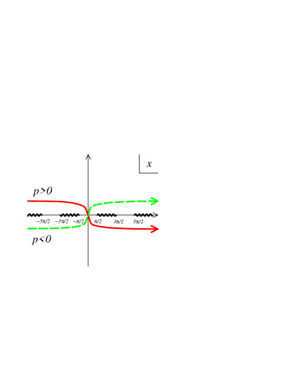
Figure 2: The red (green broken) line is the contour ${\cal C}^{+}$ for $p>0$ (${\cal C}^{-}$ for $p<0$). The imaginary $x$-axis corresponds to the Lorentzian time. Notice that an infinite number of branch cuts repeats in the Euclidean time: $\frac{\pi}{2}+2n\pi<x<\frac{3\pi}{2}+2n\pi$, $(n\in\mbox{{\bf Z}})$ along the real $x$-axis.

Here $B(p,q)\equiv\Gamma(p)\Gamma(q)/\Gamma(p+q)$ denotes Euler’s beta function. The integration contour ${\cal C}$ we choose is shown in Figure 2 [13]. As in (29), we separately evaluated the integrals of $\phi^{p}_{L,q}$ and $\phi^{p}_{R,q}$ based on the decomposition (20). For the convergence of integrals, we choose the contour ${\cal C}^{+}$ for $\phi^{p}_{L,q}$ ($p>0$ sector) and ${\cal C}^{-}$ for $\phi^{p}_{R,q}$ ($p<0$ sector). Such choice of integration contours rendered an extra damping factor $\sinh(\pi p)/{|\cosh\left(\pi\frac{p+iq}{2}\right)|^{2}}$, which improves the ultraviolet behavior of the wave function and makes it possible to take the Wick rotation sensibly. The non-trivial phase factor ${\cosh\left(\pi\frac{p-i|q|}{2}\right)}/{\cosh\left(\pi\frac{p+i|q|}{2}\right)}$ in the second term originates from the reflection amplitude, and it reduces to $(-1)^{n}$ when $q=n\in\mbox{{\bf Z}}$.

The second subtlety implies that ${\left\langle\left\langle i\omega,\alpha\right|\right.}$ is not uniquely defined in (36). This is the issue that arises in a background with horizon, equivalently, non-existence of globally definable timelike Killing vector. As such, this subtlety did not arise for the extremal NS5-brane geometry (described asymptotically by free linear dilaton theory [5, 6]) considered in [13]. In the next section, within the mini-superspace analysis for the Lorentzian two-dimensional black hole, we shall clarify this subtlety.

An alternative, sensible prescription of the analytic continuation is to define the disk one-point correlator directly via the Lorentzian Fourier transform:

$$\Big{<}\Phi^{\mbox{\scriptsize Lorentzian}}_{\omega,\alpha}\Big{>}_{\mbox{\scriptsize disk}}=\int_{-\infty}^{\infty}\mbox{d}t\,f(it,\alpha)e^{-i\omega t}~{}.$$ (39)

This is not always equivalent to the the former method elaborated above. In fact, the latter method does not necessarily assert that the boundary state constructed so is expandable in terms of the Lorentzian Ishibashi states that are analytically continued from the Euclidean ones.

3.2 Lorentzian mini-superspace wave functions

The Wick rotation of the mini-superspace eigenfunctions in the Euclidean cigar geometry (13) is not so trivial. Fortuitously, the Lorentzian eigenfunctions are already classified thoroughly in [3]. The complete basis for waves outside the black hole horizon are spanned by the following four types of eigenfunctions of the Lorentzian Klein-Gordon operator. For those with the eigenvalue $\frac{p^{2}}{4k}-\frac{\omega^{2}}{4k}+\frac{1}{4k}$ of the Klein-Gordon operator, the four eigenfunctions are

$$U^{p}_{\omega}(\rho,t) = -\frac{\Gamma^{2}(\nu_{+})}{\Gamma(1-i\omega)\Gamma(-ip)}e^{-i\omega t}(\sinh\rho)^{-i\omega}F(\nu_{+},\nu^{*}_{-};1-i\omega;-\sinh^{2}\rho)$$ (40)

$$\sim e^{-i\omega t-i\omega\ln\rho}\qquad\mbox{as}\qquad\rho\,\rightarrow\,0~{},$$

$$V^{p}_{\omega}(\rho,t) = -\frac{\Gamma^{2}(\nu^{*}_{+})}{\Gamma(1+i\omega)\Gamma(ip)}e^{-i\omega t}(\sinh\rho)^{i\omega}F(\nu^{*}_{+},\nu_{-};1+i\omega;-\sinh^{2}\rho)$$ (41)

$$\sim e^{-i\omega t+i\omega\ln\rho}\qquad\mbox{as}\qquad\rho\,\rightarrow\,0~{},$$

$$L^{p}_{\omega}(\rho,t) = e^{-i\omega t}(\sinh\rho)^{-1-ip}F(\nu^{*}_{+},\nu^{*}_{-};1+ip;-\frac{1}{\sinh^{2}\rho})$$ (42)

$$\sim e^{-\rho}e^{-ip\rho-i\omega t}\qquad\mbox{as}\qquad\rho\,\rightarrow\,\infty~{},$$

$$R^{p}_{\omega}(\rho,t) = e^{-i\omega t}(\sinh\rho)^{-1+ip}F(\nu_{+},\nu_{-};1-ip;-\frac{1}{\sinh^{2}\rho})$$ (43)

$$\sim e^{-\rho}e^{+ip\rho-i\omega t}\qquad\mbox{as}\qquad\rho\,\rightarrow\,\infty$$

with the notations

$$\nu_{\pm}=\frac{1}{2}-i\left(\frac{p}{2}\pm\frac{\omega}{2}\right)~{}.$$

These eigenfunctions are defined by the following analytic continuations of the mini-superspace Euclidean eigenfunctions:

$$U^{p}_{\omega}(\rho,t)=\left\{\begin{array}[]{ll}\phi^{p}_{n=+i\omega}(\rho,\theta=+it){}&~{}~{}(\omega>0,~{}n<0)\\ \phi^{p}_{n=-i\omega}(\rho,\theta=-it){}&~{}~{}(\omega<0,~{}n>0)\end{array}\right.$$ (46)

$$V^{p}_{\omega}(\rho,t)=\left\{\begin{array}[]{ll}\phi^{-p}_{n=-i\omega}(\rho,\theta=-it){}&~{}~{}(\omega>0,~{}n<0)\\ \phi^{-p}_{n=+i\omega}(\rho,\theta=+it){}&~{}~{}(\omega<0,~{}n>0)\end{array}\right.$$ (49)

$$L^{p}_{\omega}(\rho,t)=\phi^{p}_{L,n=i\omega}(\rho,\theta=+it)$$

$$R^{p}_{\omega}(\rho,t)=\phi^{p}_{R,n=i\omega}(\rho,\theta=+it)~{},$$ (50)

where the $n<0$ and $n>0$ ranges are mapped to $\omega>0$ and $\omega<0$, respectively.

As discussed in [3], only two out of the four eigenfunctions are linearly independent. In particular,

$$V_{\omega}^{p}(\rho,t)=U^{p*}_{\omega}(\rho,-t)\qquad\mbox{and}\qquad R_{\omega}^{p}(\rho,t)=L^{p*}_{\omega}(\rho,-t)\ .$$

The reason why we introduce the above four eigenfunctions is because they encode four possible boundary conditions (We here assume $p>0$) in the Lorentzian black hole background. Recall that, for the region outside the horizon of the eternal black hole, the boundaries consist of four segments: ‘future (past) horizon’ $t=+\infty,\,\rho=0$ ($t=-\infty,\,\rho=0$) by ${\cal H}^{+}$ (${\cal H}^{-}$), and the ‘future (past) infinity’ $t=+\infty,\,\rho=+\infty$ ($t=-\infty,\,\rho=+\infty$) by ${\cal I}^{+}$ (${\cal I}^{-}$). The four eigenfunctions $U,V,L,R$ are the ones obeying boundary conditions:

$$U^{p}_{\omega}=0~{}~{}\mbox{at}~{}{\cal H}^{-}~{},~{}~{}~{}V^{p}_{\omega}=0~{}~{}\mbox{at}~{}~{}{\cal H}^{+}~{},~{}~{}~{}L^{p}_{\omega}=0~{}(R^{p}_{\omega}=0)~{}~{}\mbox{at}~{}~{}{\cal I}^{+}~{},~{}~{}~{}R^{p}_{\omega}=0~{}(L^{p}_{\omega}=0)~{}~{}\mbox{at}~{}~{}{\cal I}^{-}$$

for $\omega>0$ ($\omega<0$). See Figure 3.

Figure 3: The boundary conditions of the Lorentzian eigenfunctions ($\omega>0$ sector). For $\omega<0$, the figures for $L$ and $R$ should be interchanged.

By Wick rotating the mini-superspace reflection relations (17), we obtain linear relations among the Lorentzian eigenfunctions:

$$U^{p}_{\omega}=L^{p}_{\omega}+{\cal R}_{0}(p,\omega)R^{p}_{\omega}\qquad\mbox{and}\qquad V^{p}_{\omega}=R^{p}_{\omega}+{\cal R}^{*}_{0}(p,\omega)L^{p}_{\omega}~{}.$$ (51)

Equivalently,

$$L^{p}_{\omega}=\frac{1}{1-|{\cal R}_{0}(p,\omega)|^{2}}\left\{U^{p}_{\omega}-{\cal R}_{0}(p,\omega)V^{p}_{\omega}\right\}\quad\mbox{and}\quad R^{p}_{\omega}=\frac{1}{1-|{\cal R}_{0}(p,\omega)|^{2}}\left\{V^{p}_{\omega}-{\cal R}^{*}_{0}(p,\omega)U^{p}_{\omega}\right\}.$$ (52)

Here, the mini-superspace reflection amplitude ${\cal R}_{0}(p,\omega)$ in Lorentzian theory is given by

$${\cal R}_{0}(p,\omega)=\frac{\Gamma(+ip)\Gamma^{2}(\nu_{+})}{\Gamma(-ip)\Gamma^{2}(\nu^{*}_{-})}\equiv-\frac{B(\nu_{+},\nu_{-})}{B(\nu_{+}^{*},\nu_{-}^{*})}\cdot\frac{\cosh\pi\left(\frac{p-\omega}{2}\right)}{\cosh\pi\left(\frac{p+\omega}{2}\right)}~{}.$$ (53)

Notice that, in sharp contrast to the Euclidean black hole, the reflection amplitude is less than unity due to the second factor:

$$|{\cal R}_{0}(p,\omega)|^{2}={\cosh^{2}\pi\left({p-\omega\over 2}\right)\over\cosh^{2}\pi\left({p+\omega\over 2}\right)}\leq 1\ .$$ (54)

The inequality is saturated at $p=\omega=0$. The inequality (54) shall play a prominent role for understanding string dynamics in the Lorentzian black hole background. The mini-superspace reflection relations for $U^{p}_{\omega}$, $V^{p}_{\omega}$ are also expressible in a form similar to the Euclidean ones. Recalling that ${\cal R}_{0}(-p,\omega){\cal R}_{0}(+p,\omega)=1$,

$$U^{-p}_{\omega}(\rho,t)={\cal R}_{0}(-p,\omega)U^{p}_{\omega}(\rho,t)\qquad\mbox{and}\qquad V^{-p}_{\omega}(\rho,t)={\cal R}^{*}_{0}(-p,\omega)V^{p}_{\omega}(\rho,t)~{},$$ (55)

while $L^{p}_{\omega}$ and $R^{p}_{\omega}$ are simply related by reflection:

$$L^{-p}_{\omega}(\rho,t)=R^{+p}_{\omega}(\rho,t)~{}.$$ (56)

Moreover, $U^{p}_{\omega}$ and $V^{p}_{\omega}$ are linearly independent except for the special kinematic regime, $\omega=0$. Notice also, in the relation (54), the reflection amplitude involves the mini-superspace contribution only, not the full-fledged stringy one.

Before proceeding further, we shall here collect explicitly relations among inner products of Lorentzian primary fields, where the inner product is defined with respect to the Lorentzian measure $\mbox{d}v_{L}=k\sinh 2\rho\mbox{d}\rho\mbox{d}t$. Taking quantum numbers $p$, $\omega$ fixed and dropping off delta function factors $2\pi\delta(p-p^{\prime})$, $2\pi\delta(\omega-\omega^{\prime})$ for notational simplicity, we have

$$(U^{p}_{\omega},U^{p}_{\omega})=(V^{p}_{\omega},V^{p}_{\omega})=N_{0}(p,\omega)~{},\qquad N_{0}(p,\omega)\equiv\frac{1+|{\cal R}_{0}(p,\omega)|^{2}}{2}$$

$$(U^{p}_{\omega},V^{p}_{\omega})={\cal R}_{0}^{*}(p,\omega)~{},$$

$$(L_{\omega}^{p},L_{\omega}^{p})=(R^{p}_{\omega},R^{p}_{\omega})=\frac{1}{2}~{},\qquad\quad(L^{p}_{\omega},R^{p}_{\omega})=0~{},$$

$$(U^{p}_{\omega},L^{p}_{\omega})=(V^{p}_{\omega},R^{p}_{\omega})=\frac{1}{2}~{},\qquad\quad(R^{p}_{\omega},U^{p}_{\omega})=(V^{p}_{\omega},L^{p}_{\omega})=\frac{{\cal R}_{0}(p,\omega)}{2}~{}.$$ (57)

The inner products involving $L^{p}_{\omega}$ and $R^{p}_{\omega}$ are readily evaluated since dominant contributions are supported in the asymptotic region $\rho\gg 0$, yielding the volume factor $2\pi\delta(0)$. The remaining inner products are then extractable from the linear relations (51), (52). We also fixed the overall normalization factors from consistency with the Euclidean inner product (15) under the $\omega\,\rightarrow\,0$ limit. Notice also that

$$N_{0}(-p,\omega)=\left|{\cal R}_{0}(-p,\omega)\right|^{2}\,N_{0}(+p,\omega)~{},$$ (58)

as is consistent with the mini-superspace reflection relation (55).

It is easy to construct the exact string vertex operators or primary states corresponding to the mini-superspace eigenfunctions $U$, $V$, $L$, $R$. To be specific, we shall consider primarily the fermionic $SL_{k}(2,\mathbb{R})/U(1)$ supercoset conformal field theory. The primary states ${|U^{p}_{\omega}\rangle}$, ${|V^{p}_{\omega}\rangle}$ are the ones of conformal weights $h=\tilde{h}=\frac{p^{2}}{4k}-\frac{\omega^{2}}{4k}+\frac{1}{4k}$ and obey the exact reflection relations

$${|U^{-p}_{\omega}\rangle}={\cal R}(-p,\omega){|U^{p}_{\omega}\rangle}~{},~{}~{}~{}{|V^{-p}_{\omega}\rangle}={\cal R}^{*}(-p,\omega){|V^{p}_{\omega}\rangle}~{},$$ (59)

and the exact reflection amplitude is given by

$${\cal R}(p,\omega)\equiv{\cal R}_{0}(p,\omega)\frac{\Gamma\Big{(}1+\frac{ip}{k}\Big{)}}{\Gamma\Big{(}1-\frac{ip}{k}\Big{)}}\ .$$ (60)

Notice that the string worldsheet effect entering through the $1/k$-correction is a pure phase. Thus, the exact reflection probability $|{\cal R}(p,\omega)|^{2}$ remains unmodified from the mini-superspace approximation result $|{\cal R}_{0}(p,\omega)|^{2}$ given in (54). We shall normalize the primary states ${|U^{p}_{\omega}\rangle}$, ${|V^{p}_{\omega}\rangle}$ ($p>0$) as

$${\langle U^{p}_{\omega}|}U^{p^{\prime}}_{\omega^{\prime}}\rangle={\langle V^{p}_{\omega}|}V^{p^{\prime}}_{\omega^{\prime}}\rangle=N(p,\omega)\,2\pi\delta(p-p^{\prime})2\pi\delta(\omega-\omega^{\prime})~{},$$

$${\langle V^{p}_{\omega}|}U^{p^{\prime}}_{\omega^{\prime}}\rangle={\cal R}^{*}(p,\omega)\,2\pi\delta(p-p^{\prime})2\pi\delta(\omega-\omega^{\prime})~{},$$ (61)

where the new normalization factor $N(p,\omega)$ is simply defined by replacing ${\cal R}_{0}$ with ${\cal R}$ in $N_{0}(p,\omega)$. The primary states ${|L^{p}_{\omega}\rangle}$, ${|R^{p}_{\omega}\rangle}$ are also definable by using the linear relations (51) or (52) but now with ${\cal R}_{0}$ replaced by ${\cal R}$. Notice that ${|U^{p}_{\omega}\rangle}$, ${|V^{p}_{\omega}\rangle}$ are the ones analytically continuable to the Euclidean primary states ${|\phi^{\pm p}_{n}\rangle}$, so often referred as the ‘Hartle-Hawking vacua’. On the other hand, the states ${|L^{p}_{\omega}\rangle}$, ${|R^{p}_{\omega}\rangle}$ does not have Euclidean counterparts. Recall that, over the Euclidean black hole background, $\phi^{p}_{L,n}$, $\phi^{p}_{R,n}$ behave badly in the vicinity of $\rho=0$ and hence ill-defined.

We also find it useful to introduce the dual basis $\widehat{{\langle U^{p}_{\omega}|}}$, $\widehat{{\langle V^{p}_{\omega}|}}$ ($p,p^{\prime}>0$) with inner products

$$\widehat{{\langle U^{p}_{\omega}|}}U^{p^{\prime}}_{\omega^{\prime}}\rangle=\widehat{{\langle V^{p}_{\omega}|}}V^{p^{\prime}}_{\omega^{\prime}}\rangle=2\pi\delta(p-p^{\prime})2\pi\delta(\omega-\omega^{\prime})~{},\qquad\widehat{{\langle U^{p}_{\omega}|}}V^{p^{\prime}}_{\omega^{\prime}}\rangle=\widehat{{\langle V^{p}_{\omega}|}}U^{p^{\prime}}_{\omega^{\prime}}\rangle=0~{}.$$ (62)

Explicitly, they are given by

$$\widehat{{\langle U^{p}_{\omega}|}}=\frac{2}{1-\left|{\cal R}(p,\omega)\right|^{2}}\left\{{\langle L^{p}_{\omega}|}-{\cal R}^{*}(p,\omega){\langle R^{p}_{\omega}|}\right\}~{},\qquad\widehat{{\langle V^{p}_{\omega}|}}=\frac{2}{1-\left|{\cal R}(p,\omega)\right|^{2}}\left\{{\langle R^{p}_{\omega}|}-{\cal R}(p,\omega){\langle L^{p}_{\omega}|}\right\}~{}.$$ (63)

As such, these dual basis obey the following exact reflection relations:

$$\widehat{{\langle U^{-p}_{\omega}|}}={\cal R}(p,\omega)\widehat{{\langle U^{p}_{\omega}|}}\qquad\mbox{and}\qquad\widehat{{\langle V^{-p}_{\omega}|}}={\cal R}(p,\omega)^{*}\widehat{{\langle V^{p}_{\omega}|}}~{}.$$ (64)

A remark is in order. The dual basis $\widehat{{\langle U^{p}_{\omega}|}}$, $\widehat{{\langle V^{p}_{\omega}|}}$ are not Wick rotatable to the Euclidean dual basis ${\langle\phi^{+p}_{n}|}$, ${\langle\phi^{-p}_{n}|}$, since $|{\cal R}(p,\omega)|=1$ for $\omega\in i\mathbb{R}$. The correct procedure would be that we first define Wick rotations for the ‘ket’ states, and then define their dual states within the Lorentzian Hilbert space. Nevertheless, one-point correlators in the Lorentzian theory, from which a set of physical observables can be computed, ought to be always analytically continuable to the one-point correlators in the Euclidean theory. Roughly speaking, ambiguities inherent to the Wick rotation of dual states drop out upon taking inner product.

Having obtained the Lorentzian primary states, we shall now construct several interesting class of boundary states for a D0-brane propagating in the black hole background. We have seen that the D0-brane propagates along the trajectory (32). The two-dimensional black hole is eternal, so, in addition to the past and the future asymptotic infinities, the causal propagation region has the past horizon ${\cal H}^{-}$ surrounding the white hole singularity and the future horizon ${\cal H}^{+}$ surrounding the black hole singularity. As such, by taking variety of possible boundary conditions, we can construct interesting class of boundary states.

3.3 Boundary state of D0-brane absorbed to future horizon

Consider first the boundary state obeying the boundary condition $\psi(\rho,t)\,\rightarrow\,0$ at the past horizon ${\cal H}^{-}$, viz. the primary states ${|U^{p}_{\omega}\rangle}$. This boundary condition is relevant for scattering of a D0-brane off the black hole, since the condition represents absorption only and no emission of the D0-brane by the black hole. D0-brane boundary state obeying such absorbing boundary condition is then expanded solely by the Ishibashi states ${}^{\widehat{U}}{\left\langle\left\langle p,\omega\right|\right.}$, ${\left.\left|p,\omega\right\rangle\right\rangle}^{U}$ that are associated with the primary states $\widehat{{\langle U^{p}_{\omega}|}}$, ${|U^{p}_{\omega}\rangle}$:

$${}_{\mbox{\scriptsize absorb}}\!{\langle B;\rho_{0},t_{0}|}=\int_{0}^{\infty}\frac{\mbox{d}p}{2\pi}\int_{-\infty}^{\infty}\frac{\mbox{d}\omega}{2\pi}\,\Psi_{\mbox{\scriptsize absorb}}(\rho_{0},t_{0};p,\omega)\,{}^{\widehat{U}}\!{\left\langle\left\langle p,\omega\right|\right.}~{},$$

$${|B;\rho_{0},t_{0}\rangle}_{\mbox{\scriptsize absorb}}=\int_{0}^{\infty}\frac{\mbox{d}p}{2\pi}\int_{-\infty}^{\infty}\frac{\mbox{d}\omega}{2\pi}\,\Psi^{*}_{\mbox{\scriptsize absorb}}(\rho_{0},t_{0};p,\omega)\,{\left.\left|p,\omega\right\rangle\right\rangle}^{U}~{}.$$ (65)

The boundary wave function $\Psi_{\mbox{\scriptsize absorb}}(\rho_{0},t_{0};p,\omega)$ is then interpreted as the disk one-point correlators:

$$\Psi_{\mbox{\scriptsize absorb}}(\rho_{0},t_{0};p,\omega) = \langle U^{p}_{\omega}\rangle_{\mbox{\scriptsize disk}}\equiv{}_{\mbox{\scriptsize absorb}}\!{\langle B;\rho_{0},t_{0}|}U^{p}_{\omega}\rangle~{},$$ (66)

The boundary wave function (66) is then obtained by taking the Wick rotation $q\,\rightarrow\,i\omega$ ($q\,\rightarrow\,-i\omega$) for $q<0$ ($q>0$) in (38) (recall (50)):

$$\Psi_{\mbox{\scriptsize absorb}}(\rho_{0},t_{0};p,\omega)=B(\nu_{+},\nu_{-})\Gamma\Big{(}1+\frac{ip}{k}\Big{)}\,e^{-i\omega t_{0}}\left[e^{-ip\rho_{0}}-\frac{\cosh\left(\pi\frac{p-\omega}{2}\right)}{\cosh\left(\pi\frac{p+\omega}{2}\right)}e^{ip\rho_{0}}\right]~{},$$ (67)

The relative minus sign in the second term of $\Psi_{\mbox{\scriptsize absorb}}(\rho_{0},t_{0};p,\omega)$ originates from the fact that the contour rotation defining the Wick rotation has opposite directions for ${\cal C}^{+}$ (suitable for $p>0$) and ${\cal C}^{-}$ (suitable for $p<0$). See figure 2. This boundary wave function (67) satisfies the exact reflection relation

$$\Psi_{\mbox{\scriptsize absorb}}(\rho_{0},t_{0};-p,\omega)={\cal R}(-p,\omega)\,\Psi_{\mbox{\scriptsize absorb}}(\rho_{0},t_{0};p,\omega)~{}.$$ (68)

With such boundary condition, the boundary wave function (67) would have no overlap with D0-brane’s trajectory (32) in the far past region $t\ll t_{0}$. In fact, the trajectory (32) starts from the past horizon ${\cal H}^{-}$ at $t=-\infty$, reaches the time-symmetric point $\rho=\rho_{0}$ at $t=t_{0}$, and then falls back the future horizon ${\cal H}^{+}$ at $t=+\infty$, while the wave function $U^{p}_{\omega}$ does not have any component outgoing from ${\cal H}^{-}$. We thus interpret that the boundary state (67) describes the future half of the classical trajectory (32). We shall hence call it the ‘absorbed D-brane’.

By utilizing the radion-tachyon correspondence, the rolling radion (as described by the boundary state (67)) is also interpretable as the rolling tachyon. In the latter interpretation, the D0-brane absorbed to the future horizon is the counterpart of the future-half S-brane [34, 9, 10], in which the tachyon rolls down the potential hill at asymptotic future $t\rightarrow+\infty$ and emits radiation.

3.4 Boundary state of D0-brane emitted from past horizon

Consider next the boundary condition: $\psi(\rho,t)\,\rightarrow\,0$ at ${\cal H}^{+}$, viz. use the basis ${\left.\left|p,\omega\right\rangle\right\rangle}^{V}$, ${}^{\widehat{V}}\!{\left\langle\left\langle p,\omega\right|\right.}$ instead of ${\left.\left|p,\omega\right\rangle\right\rangle}^{U}$, ${}^{\widehat{U}}\!{\left\langle\left\langle p,\omega\right|\right.}$. Utilizing the reflection relation, we can first rewrite (38) as the form which only includes the $p<0$ Ishibashi states by means of the reflection relation. Then, we can analytically continue the states ${|\phi^{-p}_{q}\rangle}$ ($p>0$) into ${|V^{p}_{\omega}\rangle}$. The resultant boundary state is obtained by simply replacing $p\,\rightarrow\,-p$, $\omega\,\rightarrow\,-\omega$ in (67);

$${}_{\mbox{\scriptsize emitted}}\!{\langle B;\rho_{0},t_{0}|}=\int_{0}^{\infty}\frac{\mbox{d}p}{2\pi}\int_{-\infty}^{\infty}\frac{\mbox{d}\omega}{2\pi}\,\Psi_{\mbox{\scriptsize emitted}}(\rho_{0},t_{0};p,\omega)\,{}^{\widehat{V}}\!{\left\langle\left\langle p,\omega\right|\right.}~{}.$$

$${|B;\rho_{0},t_{0}\rangle}_{\mbox{\scriptsize emitted}}=\int_{0}^{\infty}\frac{\mbox{d}p}{2\pi}\int_{-\infty}^{\infty}\frac{\mbox{d}\omega}{2\pi}\,\Psi^{*}_{\mbox{\scriptsize emitted}}(\rho_{0},t_{0};p,\omega)\,{\left.\left|p,\omega\right\rangle\right\rangle}^{V}~{}.$$ (69)

where

$$\Psi_{\mbox{\scriptsize emitted}}(\rho_{0},t_{0};p,\omega)=B(\nu^{*}_{+},\nu^{*}_{-})\Gamma\left(1-\frac{ip}{k}\right)\,e^{-i\omega t_{0}}\left[e^{ip\rho_{0}}-\frac{\cosh\left(\pi\frac{p-\omega}{2}\right)}{\cosh\left(\pi\frac{p+\omega}{2}\right)}e^{-ip\rho_{0}}\right]~{}.$$

Obviously, the emitted D0-brane wave function is the time-reversal of the absorbed D0-brane wave function (67):

$$\Psi_{\mbox{\scriptsize emitted}}(\rho_{0},t_{0};p,\omega)=\Psi^{*}_{\mbox{\scriptsize absorb}}(\rho_{0},-t_{0};p,\omega)~{}.$$

Namely, it describes the D0-brane emitted from the past horizon at asymptotic past $t=-\infty$. By the choice of the boundary condition, this boundary state (69) describes only the past half of the classical D0-brane trajectory (32).

The exact reflection relation has the form

$$\Psi_{\mbox{\scriptsize emitted}}(\rho_{0},t_{0};-p,\omega)={\cal R}^{*}(-p,\omega)\,\Psi_{\mbox{\scriptsize emitted}}(\rho_{0},t_{0};p,\omega)~{}.$$ (70)

Again, in light of the radion-tachyon correspondence, the D0-brane emitted from the past horizon is the counterpart of the past-half S-brane in tachyon rolling. The radiation creeps up the tachyon potential hill from past infinity and forms an unstable D-brane.

3.5 Boundary state of time-symmetric D0-brane

The third possible boundary state is obtainable by directly taking the analytic continuation in the disk one-point amplitudes, as we already mentioned. Recalling (50), we shall analytically continue the disk amplitudes as (assume $p>0$)

$$\langle\phi^{+p}_{q}\rangle_{\mbox{\scriptsize disk}}~{}\longrightarrow~{}\langle U^{p}_{\omega}\rangle_{\mbox{\scriptsize disk}}\qquad\mbox{and}\qquad\langle\phi^{-p}_{q}\rangle_{\mbox{\scriptsize disk}}~{}\longrightarrow~{}\langle V^{p}_{\omega}\rangle_{\mbox{\scriptsize disk}}~{}.$$ (71)

The Euclidean one-point amplitudes $\langle\phi^{\pm p}_{q}\rangle_{\mbox{\scriptsize disk}}$ are given in (38), and can be expressed in contour integrals as in (35). Recall that $\langle\phi^{p}_{L,q}\rangle_{\mbox{\scriptsize disk}}$, $\langle\phi^{p}_{R,q}\rangle_{\mbox{\scriptsize disk}}$ are prescribed by the contour integrals over ${\cal C}^{+}$, ${\cal C}^{-}$ in figure 2. We shall thus analytically continue them to the real time axis (imaginary $x$-axis). In this way, we extract the Lorentzian disk one-point amplitudes as

$$\langle U^{p}_{\omega}\rangle_{\mbox{\scriptsize disk}}=\langle U^{p}_{\omega}\rangle_{\mbox{\scriptsize disk}}^{(\mbox{\scriptsize absorb})}\qquad\mbox{and}\qquad\langle V^{p}_{\omega}\rangle_{\mbox{\scriptsize disk}}=\langle V^{p}_{\omega}\rangle_{\mbox{\scriptsize disc}}^{(\mbox{\scriptsize emitted})}~{},~{}~{}~{}$$ (72)

where the right-hand sides are simply the amplitudes associated with the ‘absorbed’ and ‘emitted’ D0-branes considered in the previous subsections and explicitly given in (67) and (69). Since $U^{p}_{\omega}$ and $V^{p}_{\omega}$ constitute the complete set of basis for Lorentzian primary fields, the amplitudes (72) would yield yet another Lorentzian D0-brane boundary states. As is obvious from the above construction, this state keeps the time-reversal symmetry manifest and reproduces the entire classical trajectory (32), that is, it describes a D0-brane emitted from the past horizon and reabsorbed to the future horizon. From the viewpoint of the boundary conformal theory, this would be considered the most natural one since it captures the entire classical trajectory of the D0-brane. In the radion-tachyon correspondence, this state is the counterpart of the full S-brane [34, 1].

Explicitly, the time-symmetric boundary states are given by

$${}_{\mbox{\scriptsize symm}}\!{\langle B;\rho_{0},t_{0}|}={}_{\mbox{\scriptsize absorb}}\!{\langle B;\rho_{0},t_{0}|}+{}_{\mbox{\scriptsize emitted}}\!{\langle B;\rho_{0},t_{0}|}$$

$$\hskip 56.9055pt=\int_{0}^{\infty}\frac{\mbox{d}p}{2\pi}\int_{-\infty}^{\infty}\frac{\mbox{d}\omega}{2\pi}\,\left[2\Psi_{\mbox{\scriptsize symm}}(\rho_{0},t_{0};p,\omega)\,{}^{L}\!{\left\langle\left\langle p,\omega\right|\right.}+2\Psi^{*}_{\mbox{\scriptsize symm}}(\rho_{0},-t_{0};p,\omega)\,{}^{R}\!{\left\langle\left\langle p,\omega\right|\right.}\right]$$

$${|B;\rho_{0},t_{0}\rangle}_{\mbox{\scriptsize symm}}={|B;\rho_{0},t_{0}\rangle}_{\mbox{\scriptsize absorb}}+{|B;\rho_{0},t_{0}\rangle}_{\mbox{\scriptsize emitted}}$$

$$\hskip 56.9055pt=\int_{0}^{\infty}\frac{\mbox{d}p}{2\pi}\int_{-\infty}^{\infty}\frac{\mbox{d}\omega}{2\pi}\,\left[2\Psi^{*}_{\mbox{\scriptsize symm}}(\rho_{0},t_{0};p,\omega)\,{\left.\left|p,\omega\right\rangle\right\rangle}^{L}+2\Psi_{\mbox{\scriptsize symm}}(\rho_{0},-t_{0};p,\omega)\,{\left.\left|p,\omega\right\rangle\right\rangle}^{R}\right]~{},$$ (73)

where

$$\Psi_{\mbox{\scriptsize symm}}(\rho_{0},t_{0};p,\omega)=B(\nu_{+},\nu_{-})\Gamma\left(1+\frac{ip}{k}\right)\,e^{-ip\rho_{0}-i\omega t_{0}}$$

and ${}^{L}\!{\left\langle\left\langle p,\omega\right|\right.}$, ${\left.\left|p,\omega\right\rangle\right\rangle}^{L}$, ${}^{R}\!{\left\langle\left\langle p,\omega\right|\right.}$, ${\left.\left|p,\omega\right\rangle\right\rangle}^{R}$ are the Ishibashi states constructed over the primary states ${\langle L^{p}_{\omega}|}$, ${|L^{p}_{\omega}\rangle}$, ${\langle R^{p}_{\omega}|}$, ${|R^{p}_{\omega}\rangle}$, respectively. One can readily check that the second lines in (73) are indeed correct by evaluating the disk one-point amplitudes from them. For instance, using (57), we obtain

$$\langle U^{p}_{\omega}\rangle_{\mbox{\scriptsize disk}}^{(\mbox{\scriptsize symm})} = {}_{\mbox{\scriptsize symm}}\!{\langle B;\rho_{0},t_{0}|}U^{p}_{\omega}\rangle$$

$$= \Psi_{\mbox{\scriptsize symm}}(\rho_{0},t_{0};p,\omega)+{\cal R}(p,\omega)\Psi^{*}_{\mbox{\scriptsize symm}}(\rho_{0},-t_{0};p,\omega)$$

$$= B(\nu_{+},\nu_{-})\Gamma\left(1+\frac{ip}{k}\right)e^{-i\omega t_{0}}\,\left[e^{-ip\rho_{0}}-\frac{\cosh\left(\pi\frac{p-\omega}{2}\right)}{\cosh\left(\pi\frac{p+\omega}{2}\right)}e^{ip\rho_{0}}\right]$$

$$= \langle U^{p}_{\omega}\rangle^{(\mbox{\scriptsize absorb})}_{\mbox{\scriptsize disk}}\equiv{}_{\mbox{\scriptsize absorb}}\!{\langle B;\rho_{0},t_{0}|}U^{p}_{\omega}\rangle~{}.$$

Other one-point amplitudes can be checked analogously.

Two remarks are in order. First, notice that, though the disk one-point amplitudes are, the symmetric boundary states (73) by themselves are not analytically continuable to the Euclidean boundary state (38). This should not be surprising as the Lorentzian Hilbert space is generated by twice as many generators as the Euclidean theory. In other words, the Lorentzian bases ${|U^{p}_{\omega}\rangle}$, ${|V^{p}_{\omega}\rangle}$ correspond to ${|\phi^{p}_{n}\rangle}$, ${|\phi^{-p}_{n}\rangle}$ in the Euclidean theory, which were however linearly dependent due to the reflection relation. Nevertheless, the boundary state (73) is a consistent one and yields disk one-point amplitudes that can be correctly continued to the Euclidean ones. Second, the full Lorentzian Hilbert space is decomposed as

$${\cal H}={\cal H}^{U}\oplus{\cal H}^{V}\qquad\mbox{and}\qquad\widehat{{\cal H}}=\widehat{{\cal H}^{U}}\oplus\widehat{{\cal H}^{V}}~{},$$ (74)

where ${\cal H}^{U}$ (${\cal H}^{V}$) is spanned by ${|U^{p}_{\omega}\rangle}$ , ($\,{|V^{p}_{\omega}\rangle}\,$) and their descendants. The dual space $\widehat{{\cal H}^{U}}$ ($\widehat{{\cal H}^{V}}$) is similarly spanned by $\widehat{{\langle U^{p}_{\omega}|}}$, ($\widehat{{\langle V^{p}_{\omega}|}}$). Here, the Hilbert subspaces ${\cal H}^{U}$, $\widehat{{\cal H}^{U}}$ (${\cal H}^{V}$, $\widehat{{\cal H}^{V}}$) correspond to the boundary condition $\psi(\rho,t)\,\rightarrow\,0$ at ${\cal H}^{-}$ (${\cal H}^{+}$). The ‘absorbed’ and ‘emitted’ D0-brane boundary states (67), (69) are consistent only in the subspaces ${\cal H}^{U}$, ${\cal H}^{V}$ ($\widehat{{\cal H}^{U}}$, $\widehat{{\cal H}^{V}}$), while the ‘symmetric’ D0-brane boundary state (73) is well-defined in the entire Hilbert space ${\cal H}$ ($\widehat{{\cal H}}$). We thus have simple relations

$${|B;\rho_{0},t_{0}\rangle}_{\mbox{\scriptsize absorb}}=P_{U}\,{|B;\rho_{0},t_{0}\rangle}_{\mbox{\scriptsize symm}}\qquad \qquad{}_{\mbox{\scriptsize absorb}}\!{\langle B;\rho_{0},t_{0}|}={}_{\mbox{\scriptsize symm}}\!{\langle B;\rho_{0},t_{0}|}\,\widehat{P_{U}}~{},$$ and

$${|B;\rho_{0},t_{0}\rangle}_{\mbox{\scriptsize emitted}}=P_{V}\,{|B;\rho_{0},t_{0}\rangle}_{\mbox{\scriptsize symm}}\qquad \qquad{}_{\mbox{\scriptsize emitted}}\!{\langle B;\rho_{0},t_{0}|}={}_{\mbox{\scriptsize symm}}\!{\langle B;\rho_{0},t_{0}|}\,\widehat{P_{V}}~{},$$ and (75)

where $P_{U,V}$ ($\widehat{P_{U,V}}$) denotes projection of the Hilbert space ${\cal H}$ to ${\cal H}^{U,V}$ ($\widehat{{\cal H}^{U,V}}$).

4 Radiation out of D0-Brane Rolling in the Black Hole Background

In the background of the black hole, the D0-brane moves along the geodesic and we have constructed a variety of boundary states describing the geodesic motion, specified by appropriate boundary conditions.

Both by gravity and by strong string coupling gradient, the D$p$-brane is pulled in and finds its minimum energy and mass at the location of the NS5-brane. The D$p$-brane is supersymmetric in flat spacetime, but preserves no supersymmetry in black NS5-brane background. Even in extremal NS5-brane background, until the D$p$-brane dissociates into the NS5-brane and form a non-threshold bound-state, the spacetime supersymmetry is completely broken. In these respects,the D$p$-brane propagating in the NS5-brane background is much like excited D$p$-brane (many excited open strings attached on it) in flat spacetime. Decay of the latter via closed string emission was studied extensively for $p=1$ [35]: the decay spectrum was found to match exactly with the Hawking radiation of the non-extremal black hole made out of these excited D-branes, and the effective temperature of excited open string modes agrees exactly with the Hawking temperature. In this section, we shall find certain analogous results for the closed string radiation off the rolling D0-brane, though special features also arise.

As the D0-brane is pulled in, acceleration would grow and radiate off the binding energy into closed string modes. Details of the radiation spectra would differ for different choice of the boundary conditions, viz. for different boundary states of the D0-brane. In this section, as a probe of the black hole geometry and D-brane dynamics therein, we shall analyze spectral distribution of the closed string radiation off the rolling D0-particle.

By applying the optical theorem, the radiation rate during the radion-rolling process is obtainable as the imaginary part of the annulus amplitude in the closed string channel. Denote the differential number density $\mbox{d}{\cal N}(p,M)$ of the radiation at a fixed value of the radial momentum $p$ and the mass-level $M$. By the definition of the D-brane boundary state, the radiation number density $\mbox{d}{\cal N}$ is then given in terms of the boundary wave functions:

$$\mbox{d}{\cal N}(p,M) := {\mbox{d}p\over 2\pi}{\mbox{d}M\over(2\pi)^{d}}\int{\mbox{d}\omega}\,\Big{<}\Psi(\omega,p,M)\Big{|}\delta(L_{0}+\overline{L}_{0})\Big{|}\Psi(\omega,p,M)\Big{>}$$ (76)

$$= \frac{\mbox{d}p}{2\pi}\frac{\mbox{d}M}{(2\pi)^{d}}\frac{1}{2\omega(p,M)}\,\Big{|}\Psi(p,\omega(p,M))\Big{|}^{2}~{}.$$

Here, $\omega,p$ are the energy and the radial momentum in two-dimensional Lorentzian background, $M$ is the total mass (conformal weight) of the remaining subspaces of dimension $d$ (including mass gap), $\Psi(\omega,p,M)$ is the boundary wave function (including that of the remaining subspace), and $\omega(p,M)(>0)$ is the on-shell energy of the radiated closed string state determined by the on-shell condition $L_{0}+\overline{L}_{0}=0$ including the ghost contribution. From the kinematical consideration, it is obvious that the differential number density (76) is nonzero only when the D-brane is rolling. Of particular physical interest is the spectral distribution in the phase-space, as measured by the independent moments, e.g.

$$\Big{<}\omega^{m}M^{n}\Big{>} = \int\frac{\mbox{d}p}{2\pi}\frac{\mbox{d}M}{(2\pi)^{d}}\omega^{m}(p,M)M^{n}\frac{1}{2\omega(p,M)}\Big{|}\Psi(p,\omega(p,M))\Big{|}^{2}$$

for $m,n=0,1,2,\cdots$. We shall evaluate these spectral observables by first evaluating the integral over the radial momentum $p$ by saddle-point approximation. In doing so, we pay particular attention to the asymptotic behavior as the mass-level $M$ becomes asymptotically large. We shall then evaluate the integral over the mass-level (conformal weight) $M$, and extract the spectral observables.

Consider the boundary state (67) describing a D0-brane absorbed by the future horizon. The radiation emitted by the D0-brane is decomposable into ‘incoming’ (toward the horizon) and ‘outgoing’ (toward the null infinity) components in the far future. The positive energy sector is expanded by the wave function $U^{p}_{\omega}$, and has the following asymptotic behavior at $t\rightarrow+\infty$:

$$U^{p}_{\omega}(\rho,t)\sim e^{-i\omega\ln\rho-i\omega t}+d(p,\omega)e^{-\rho}e^{+ip\rho-i\omega t}\qquad\mbox{where}\qquad|d(p,\omega)|\sim e^{-\pi p}~{}.$$ (77)

Here, we assumed $\omega\sim M\gg 0$. The first and the second terms correspond to the incoming wave supported around $\rho=0$ and the outgoing wave supported in the region $\rho\sim+\infty$, respectively. The damping factor $d(p)$ originates from the exact reflection amplitude ${\cal R}(p,\omega)$. (See (51), (52).) To obtain the radiation number density, we need to evaluate $\left|\Psi(p,\omega)\right|^{2}\times|U^{p}_{\omega}(\rho,t)|^{2}$. At far future infinity, the interference term in $|U^{p}_{\omega}|^{2}$ drops off upon taking the $p$-integral. Therefore, after integrating over the radial momentum $p$, the partial radiation distribution is seen to consist of the ‘incoming’ and ‘outgoing’ parts:

$${\cal N}(M)_{\mbox{\scriptsize in}} \equiv \int_{0}^{M}\mbox{d}M{\mbox{d}{\cal N}_{\mbox{\scriptsize in}}\over\mbox{d}M}=\int_{0}^{\infty}\frac{\mbox{d}p}{2\pi}\frac{1}{2\omega(p,M)}\Big{|}\Psi(p,\omega(p,M))\Big{|}^{2}$$

$${\cal N}(M)_{\mbox{\scriptsize out}} \equiv \int_{0}^{M}\mbox{d}M{\mbox{d}{\cal N}_{\mbox{\scriptsize out}}\over\mbox{d}M}=\int_{0}^{\infty}\frac{\mbox{d}p}{2\pi}\frac{1}{2\omega(p,M)}\Big{|}d(p)\Big{|}^{2}\Big{|}\Psi(p,\omega(p,M))\Big{|}^{2}~{}.$$ (78)

We shall now evaluate the branching ratio between the two radiation rates (78) with emphasis on possible string worldsheet effects. To this end, consider the conformal field theory defined by $SL(2;\mathbb{R})/U(1)\times{\cal M}$, where $SL(2;\mathbb{R})/U(1)$ denotes the (super)coset model and ${\cal M}$ denotes a unitary (super)conformal field theory of central charge $c_{\cal M}$. Such (super)conformal field theory covers a variety of interesting string theory backgrounds. For the fermionic string, superconformal invariance asserts that the central charge ought to be critical:

$$3\Big{(}1+\frac{2}{k}\Big{)}+c_{\cal M}=15~{},$$

where $k$ denotes the level of the super $SL(2;\mathbb{R})$ current algebra. If the background describes a stack of black NS5-branes, ${\cal M}=SU(2)_{k}\times\mathbb{R}^{5}$ where $k$ equals to the NS5-brane charge. Likewise, for the bosonic string case, conformal invariance asserts that the central charge should take the critical value:

$$2+\frac{6}{\kappa-2}+c_{{\cal M}}=26~{},$$ (79)

where now $\kappa$ refers to the level of the bosonic $SL(2;\mathbb{R})$ current algebra. For the background describing the black hole in two-dimensional string theory, ${\cal M}$ is empty and $\kappa$ should be set to $9/4$.

It would be illuminating to analyze the branching ratio for the ‘rolling closed string’, viz. a closed string state of fixed transverse mass $M$ and radial momentum $p$ propagating in black hole geometry. The branching ratio is simply given by the reflection amplitude (see (60)):

$$\left.{{\cal N}_{\rm out}(p,\omega)\over{\cal N}_{\rm in}(p,\omega)}\right|_{\rm closed\,string}=|{\cal R}(p,\omega)|^{2}={\cosh^{2}\pi\left(\omega-p\over 2\right)\over\cosh^{2}\pi\left({\omega+p\over 2}\right)}~{}.$$ (80)

As emphasized below (60), string worldsheet effects are present for the reflection amplitude ${\cal R}$ itself but, being an overall phase, it drops out of (80). The $k$-dependence enters in the branching ratio (80) only through the on-shell dispersion relation $\omega=\sqrt{p^{2}+2kM^{2}}$. For two-dimensional case, first studied in [3] and [39], $k=1/2$, $M=0$ and $\omega=p$, so the scattering probability is exponentially suppressed as the energy increases.

For a fixed transverse mass $M$ and the forward radial momentum $p$, the reflection probability of the infalling D0-brane is given precisely by the same result as (80):

$$\left.{{\cal N}_{\rm out}(p,\omega)\over{\cal N}_{\rm in}(p,\omega)}\right|_{\rm D0-brane}=|{\cal R}(p,\omega)|^{2}={\cosh^{2}\pi\left(\omega-p\over 2\right)\over\cosh^{2}\pi\left({\omega+p\over 2}\right)}~{}.$$ (81)

This is simply because back-scattering of the boundary wave function originates from that of the closed string wave function: roughly speaking, the boundary wave function is defined by overlap of the closed string wave function with the classical trajectory of the D0-brane.

Radiation out of the falling D0-brane is coherent, so we integrate over the radial momentum $p$ as in (78) in extracting the branching ratio. We shall first analyze the partial radiation distribution at large mass-level, $M\rightarrow\infty$. More precisely, we shall examine asymptotic behavior of ${\cal N}(M)$ multiplied by the phase-space ‘degeneracy factor’ $\rho(M)\sim e^{\frac{1}{2}M\beta_{\rm Hg}}$, where $\beta_{\rm Hg}$ denotes inverse of the Hagedorn temperature. The closed string states that couple to the boundary states are left-right symmetric, so we need to take the square root of the usual degeneracy factor in the closed string sector. Here, inverse of the Hagedorn temperature is given by

$$\beta_{\rm Hg}=4\pi\sqrt{1-\frac{1}{2k}}~{},~{}~{}~{}$$ (82)

for the superstring theory, and

$$\beta_{\rm Hg}=4\pi\sqrt{2-\frac{1}{2(\kappa-2)}}~{},~{}~{}~{}$$ (83)

for the bosonic string theory, where the $1/k$ $(1/\kappa)$-correction is interpreted as the string worldsheet effects of the two-dimensional background. These results are derivable from the Cardy formula with the ‘effective central charge’ $c_{\mbox{\scriptsize eff}}=c-24h_{\mbox{\scriptsize min}}$ [40], where $h_{\mbox{\scriptsize min}}$ refers to the lowest conformal weight of normalizable primary states.

4.1 Radiation distribution in superstring theory

Begin with the spectral distribution in superstring theories. We shall focus exclusively on the NS-NS sector of the radiation and defer the analysis of the R-R sector to section 6. The on-shell condition of closed string state in NS-NS sector is given by

$$-\frac{\omega^{2}}{4k}+\frac{p^{2}}{4k}+\frac{1}{4k}+\Delta_{\cal M}=\frac{1}{2}~{},$$ (84)

where $\Delta_{\cal M}$ denotes the conformal weight of the ${\cal M}$-part. The on-shell energy is given by

$$\omega\equiv\omega(p,M)=\sqrt{p^{2}+2kM^{2}}\qquad\mbox{where}\qquad M^{2}\equiv 2\left(\Delta_{\cal M}+\frac{1}{4k}-\frac{1}{2}\right)~{}.$$

Consider now a D0-brane propagating outside the black hole and absorbed into the future horizon. The relevant boundary wave function was constructed in (67) and, from them, the differential radiation number distributions (78) can be computed. At large $\omega$ and $p$, using Stirling’s approximation, we find that

$${\cal N}(M)_{\mbox{\scriptsize in}} = \int_{0}^{\infty}\frac{\mbox{d}p}{2\pi}\frac{1}{2\omega(p,M)}\,\Big{|}\Psi_{\rm absorb}(\rho_{0},t_{0};p,\omega(p,M))\Big{|}^{2}$$ (85)

$$\sim {1\over M}\int_{0}^{\infty}{\mbox{d}p}\,e^{+\pi\left(1-\frac{1}{k}\right)p-\pi\sqrt{p^{2}+2kM^{2}}}~{}$$

$${\cal N}(M)_{\mbox{\scriptsize out}} = \int_{0}^{\infty}\frac{\mbox{d}p}{2\pi}\,\Big{|}d(p,\omega(p,M))\Big{|}^{2}\,\frac{1}{2\omega(p,M)}\Big{|}\Psi_{\rm absorb}(\rho_{0},t_{0};p,\omega(p,M))\Big{|}^{2}$$ (86)

$$\sim {1\over M}\int_{0}^{\infty}{\mbox{d}p}\,e^{-\pi\left(1+\frac{1}{k}\right)p-\pi\sqrt{p^{2}+2kM^{2}}}~{}.$$

In the second lines, we have taken $M$ large, viz. $\omega\gg p\gg 1$, and keep the leading terms only. Thus, for each fixed but large $M$, the partial number distributions take the forms:

$${\cal N}(M)_{\mbox{\scriptsize in}}\sim\int_{0}^{\infty}\mbox{d}p\,\sigma_{\mbox{\scriptsize in}}(p)e^{-\frac{1}{2}\beta_{\rm Hw}M}\qquad\mbox{and}\qquad N(M)_{\mbox{\scriptsize out}}\sim\int_{0}^{\infty}\mbox{d}p\,\sigma_{\mbox{\scriptsize out}}(p)e^{-\frac{1}{2}\beta_{\rm Hw}M}~{},$$ (87)

where

$$\beta_{\rm Hw}=2\pi\sqrt{2k}~{},$$ (88)

is the inverse Hawking temperature of the fermionic two-dimensional black hole. As discussed above, the radiation off the D-brane in NS5-brane background is analogous to the decay of excited D-brane in flat ambient spacetime. Indeed, asymptotic expression (87) suggests that open string excitations of energy $M$ on the rolling D0-brane are populated as the distribution function $\exp(-{1\over 2}\beta_{\rm Hw}M)$ and decay into closed string radiation. In this interpretation, the distribution function encodes change of available states for open string excitations on the D0-brane after emitting radiations of energy $M$. Curiously, ‘effective temperature’ of the excited closed strings is set by the Hawking temperature of the nonextremal NS5-brane, not that of a black hole that would have been made of the D0-brane. It is tempting to interpret this as indicating that the D0-brane represents a class of possible excitation modes of the black NS5-brane. The closed string states of energy $M$ emitted by the D0-brane are certainly coherent, but according to this interpretation, they still can be recasted in effective thermal distribution set by the Hawking temperature of the two-dimensional black hole. In the next subsection, we shall account for the origin of such effective thermal behavior of the rolling D0-brane from the viewpoints of Euclidean cylinder amplitude between D1-brane, extending the argument of [3] for the Hawking radiation of closed strings in the black hole background.

The functions $\sigma_{\rm in}$ and $\sigma_{\rm out}$ are interpretable as the black hole ‘greybody’ factors for incoming and outgoing parts of the radiation. The factor 1/2 in the exponent of the Boltzmann distribution function reflects the fact that only left-right symmetric closed string states can appear in the boundary states and the radiated closed string modes.

The ‘greybody factors’ $\sigma_{*}(p)$ depend on the radial momentum $p$ exponentially, so the radiation distribution would be modified once the radial momentum $p$ is integrated out. Below, we shall show this explicitly. We are primarily interested in keeping track of string worldsheet effects set by the value of the level $k$. We shall consider different ranges of the level $k$ separately, and focus on the asymptotic behaviors at large $M$ via the saddle point methods.

(i) $k>1$:

This is the case for the black NS5-brane background. Consider first the incoming part. Since $1-\frac{1}{k}>0$, the dominant contribution in the $p$-integral arises from the saddle point:

$$p\sim p_{*}=\frac{k-1}{\sqrt{1-\frac{1}{2k}}}M~{}.$$

Substituting this to (85), we obtain

$${\cal N}(M)_{\mbox{\scriptsize in}}\sim e^{-2\pi M\sqrt{1-\frac{1}{2k}}}=e^{-\frac{1}{2}M\beta_{\rm Hg}}~{},$$ (89)

up to pre-exponential powers of $M$. Taking account of the density of states $\rho(M)\sim e^{\frac{1}{2}M\beta_{\rm Hg}}$, we find that $\rho(M){\cal N}(M)_{\mbox{\scriptsize in}}$ scales with powers of $M$, and is independent of $k$. More explicitly, for the black NS5-brane ${\cal M}=SU(2)_{k}\times\mathbb{R}^{5}$, the incoming radiation distribution of the D$p$-brane parallel to the NS5-brane yields

$${\cal N}(M)_{\mbox{\scriptsize in}} \sim {1\over M}\int{\mbox{d}^{5-p}{\bf k}_{\perp}\over(2\pi)^{5-p}}\int_{0}^{\infty}{\mbox{d}p}\,e^{\pi(1-\frac{1}{k})p-\pi\sqrt{p^{2}+2k(M^{2}+{\bf k}_{\perp}^{2})}}$$

$$\sim M^{2-\frac{{p}}{2}}\,e^{-2\pi M\sqrt{1-\frac{1}{2k}}}\ .$$

Taking account of the density of states $\rho(M)\sim M^{-3}e^{2\pi M\sqrt{1-\frac{1}{2k}}}$, the average radiation number distribution is given by

$$\frac{\overline{{\cal N}}_{\mbox{\scriptsize in}}}{V_{p}}\sim\int^{M_{\rm D}}{\mbox{d}M\over M}\,M^{-\frac{p}{2}}\qquad\mbox{where}\qquad M_{\rm D}\sim{\cal O}({1\over g_{\rm st}})\ .$$ (90)

This result coincides with the computations of [36, 37], and corroborates with the radion-tachyon correspondence. Interestingly, the incoming part of the radiation number distribution in the the nonextremal NS5-brane background is exactly the same as the distribution in the extremal NS5-brane background. Later, we shall examine carefully taking the extremal limit and its consequence in section 7. As in the extremal case, (90) implies that nearly all the D0-brane potential energy is released into closed string radiations before it falls into the black hole.

On the other hand, for the outgoing radiation, the far infrared $p\sim 0$ dominates the momentum integral. We thus obtain

$${\cal N}(M)_{\mbox{\scriptsize out}}\sim e^{-2\pi M\sqrt{\frac{k}{2}}}=e^{-\frac{1}{2}M\beta_{\rm Hw}}~{},$$

displaying effective thermal distribution set by the Hawking temperature. Taking account of the density of states,

$$\rho(M){\cal N}(M)_{\mbox{\scriptsize out}}\sim e^{\frac{1}{2}M\left(\beta_{\rm Hg}-\beta_{\rm Hw}\right)}=e^{2\pi M\left(\sqrt{1-\frac{1}{2k}}-\sqrt{\frac{k}{2}}\right)}~{}.$$

This is ultraviolet finite for any $k$ since

$$\left(1-\frac{1}{2k}\right)-\frac{k}{2}=-\frac{1}{2k}\left(k-1\right)^{2}<0~{}.$$ (91)

We thus conclude that the radiation number distribution is mostly in the incoming part:

$$\left.{{\cal N}_{\rm out}(M)\rho(M)\over{\cal N}_{\rm in}(M)\rho(M)}\right|_{\rm falling\,\,D0}\sim{e^{-{1\over 2}\beta_{\rm Hw}M}\over e^{-{1\over 2}\beta_{\rm Hg}M}}=e^{2\pi M\left(\sqrt{1-{1\over 2k}}-\sqrt{k\over 2}\right)}\ll 1\ .$$

Intuitively, this may be understood as follows: for the absorbed boundary state, the boundary condition is such that the D0-brane flux is directed from past null infinity to the future horizon. This also corroborates the observation that $T_{t\rho}$-component of D0-brane’s energy-momentum tensor is nonzero and increases monotonically as the D0-brane approaches the future horizon. The outgoing part of the distribution is exponentially small compared to the incoming part and exhibits effective thermal distribution at the Hawking temperature. Notice that, despite being so, this outgoing part has nothing to do with the Hawking radiation of the black hole. The latter is the feature of the background by itself. A priori, the outgoing radiation could be in a distribution characterized by a temperature different from the Hawking temperature. As mentioned above, it is tempting to interpret coincidence of the two temperatures as a consequence of maintaining equilibrium between the black NS5-brane and the D0-brane.

(ii) $\frac{1}{2}<k\leq 1$:

This is the regime which includes the conifold geometry at $k=1$. Since $1-\frac{1}{k}\leq 0$, the dominant contribution to the momentum integral is from $p\sim 0$, not only for the outgoing radiation but also for the incoming one. We thus obtain

$${\cal N}(M)_{\mbox{\scriptsize in}}\sim{\cal N}(M)_{\mbox{\scriptsize out}}\sim e^{-2\pi M\sqrt{\frac{k}{2}}}\equiv e^{-\frac{1}{2}M\beta_{\rm Hw}}~{},$$ (92)

viz. both are in effective thermal distribution set by the Hawking temperature. All spectral moments are manifestly ultraviolet finite since, at large $M$, exponential growth of the density of the final closed string states is insufficient to overcome the suppression by the distribution. Thus,

$${{\cal N}_{\rm out}(M)\rho(M)\over{\cal N}_{\rm in}(M)\rho(M)}\Big{|}_{\rm falling\,D0}\sim 1\ .$$

We interpret this as indicating that the D0-brane does not radiate off most of its energy before falling into the horizon.

(iii) $k=\frac{1}{2}$ :

This special case corresponds to empty ${\cal M}$. The two-dimensional background permits no transverse degrees of freedom of the string. The physical spectrum includes massless tachyon only, with $M=0$ and $\rho(M)=1$. We now have a crucial difference from the previous cases for the on-shell configurations. The radial momentum $p$ is fixed by the on-shell condition as $\omega=\pm p$, so it should not be integrated over for the final states. Consequently, we cannot decompose the radiation distribution into incoming and outgoing radiations, and only the total distribution is physically relevant.

We thus obtain the following large $\omega$ behavior of the radiation distribution:

$${\cal N}(\omega)\sim e^{-2\pi\omega}\equiv e^{-\omega\beta_{\rm Hw}}~{}.$$ (93)

Again, we have found effective thermal distribution at the Hawking temperature! Notice the absence of extra 1/2-factor in contrast to the previous regimes. This is not a contradiction. In the present case, the transverse oscillators are absent and the string behaves as a point particle. Again, the D0-brane does not radiate off most of its energy before falling across the black hole horizon.

4.2 Radiation distribution in bosonic string theory

The analysis for the bosonic string case proceeds quite the same route. The boundary state for the infalling D0-brane includes the string worldsheet correction factor $\Gamma\left(1+i\frac{p}{\kappa-2}\right)$, where again $\kappa$ refers to the level of bosonic $SL(2;\mathbb{R})/U(1)$ coset model. The on-shell condition now reads

$$-\frac{\omega^{2}}{4\kappa}+\frac{p^{2}}{4(\kappa-2)}+\frac{1}{4(\kappa-2)}+\Delta_{\cal M}=1~{},$$ (94)

where $\Delta_{\cal M}$ denotes the conformal weight in the ${\cal M}$-sector. This is solved by

$$\omega\equiv\omega(p,M)=\sqrt{\frac{\kappa}{\kappa-2}p^{2}+2\kappa M^{2}}\qquad\mbox{where}\qquad M^{2}\equiv 2\left(\Delta_{\cal M}+\frac{1}{4(\kappa-2)}-1\right)~{}.$$ (95)

The partial radiation number distribution at large $M$ limit is given by:

$${\cal N}(M)_{\mbox{\scriptsize in}}\sim{1\over M}\int_{0}^{\infty}{\mbox{d}p}\,e^{+\pi\left(1-\frac{1}{\kappa-2}\right)p-\pi\sqrt{\frac{\kappa}{\kappa-2}p^{2}+2\kappa M^{2}}}~{}.$$ (96)

$${\cal N}(M)_{\mbox{\scriptsize out}}\sim{1\over M}\int_{0}^{\infty}{\mbox{d}p}\,e^{-\pi\left(1+\frac{1}{\kappa-2}\right)p-\pi\sqrt{\frac{\kappa}{\kappa-2}p^{2}+2\kappa M^{2}}}~{}.$$ (97)

Thus, as in the superstring case, there can arise several distinct behaviors depending on how stringy the background is.

(i) $\kappa>3$:

Consider first the incoming radiation part. Since $1-\frac{1}{\kappa-2}>0$, the dominant contribution to the momentum integral in (96) is from the saddle point

$$p\sim p_{*}=\frac{\kappa-3}{\sqrt{2-\frac{1}{2(\kappa-2)}}}M~{}.$$

We thus obtain, up to pre-exponential powers of $M$,

$${\cal N}(M)_{\mbox{\scriptsize in}}\sim e^{-2\pi M\sqrt{2-\frac{1}{2(\kappa-2)}}}\,=\,e^{-\frac{1}{2}M\beta_{\rm Hg}}~{},$$

where $\beta_{\rm Hg}$ denotes the Hagedorn temperature of the bosonic string theory (83). In this way, we again find the power-law behavior of $\rho(M){\cal N}(M)_{\mbox{\scriptsize in}}$ at large $M$, independent of the level $\kappa$.

For the outgoing radiation part, again the $p\sim 0$ dominates the momentum integral in (97). The result is

$${\cal N}(M)_{\mbox{\scriptsize out}}\sim e^{-2\pi M\sqrt{\frac{\kappa}{2}}}=e^{-\frac{1}{2}M\beta_{\rm Hw}}~{}.$$

Here,

$$\beta_{\rm Hw}\equiv 2\pi\sqrt{2\kappa}$$

is the Hawking temperature of the bosonic two-dimensional black hole. We then obtain

$$\rho(M){\cal N}(M)_{\mbox{\scriptsize out}}\sim e^{\frac{1}{2}\left(\beta_{\rm Hg}-\beta_{\rm Hw}\right)M}=e^{2\pi M\left[\sqrt{2-\frac{1}{2(\kappa-2)}}-\sqrt{\frac{\kappa}{2}}\right]}~{}.$$

As in the superstring case, the exponent is always negative definite:

$$\left(2-\frac{1}{2(\kappa-2)}\right)-\frac{\kappa}{2}=-\frac{\left(\kappa-3\right)^{2}}{2(\kappa-2)}\leq 0~{}.$$

so the outgoing radiation distribution (as well as spectral moments) is manifestly ultraviolet finite.

Physical interpretation of the above results is the same as the superstring case: The D0-brane falling into the black hole has nonzero component $T_{t\rho}$ of the energy-momentum tensor, and entails that dominant part of the closed string radiation is incoming toward the future horizon. The outgoing part of the radiation is exponentially suppressed, and is in effective thermal distribution set by the Hawking temperature. Again, this distribution is distinct from the Hawking radiation of the two-dimensional black hole. As for the fermionic string, the branching ratio is exponentially suppressed.

(ii) $\frac{9}{4}<\kappa\leq 3$:

In this regime, $1-\frac{1}{\kappa-2}<0$ and the momentum integrals for both incoming and outgoing radiation distributions are dominated by $p\sim 0$:

$${\cal N}(M)_{\mbox{\scriptsize in}}\sim{\cal N}(M)_{\mbox{\scriptsize out}}\sim e^{-2\pi M\sqrt{\frac{\kappa}{2}}}\equiv e^{-\frac{1}{2}M\beta_{\rm Hw}}~{}.$$

Both are in effective thermal distribution at the Hawking temperature, and all spectral moments are manifestly ultraviolet finite since, at large $M$, the growth of the density of state does not overcome the suppression by the distribution. The branching ratio remains order unity.

(iii) $\kappa=\frac{9}{4}$ :

This is the most familiar situation: black hole in two-dimensional bosonic string theory, originally studied in [2]. The physical spectrum of closed string consists only of the massless tachyon, so we again need to set $M=0$ and $\rho(M)=1$. The calculation is slightly more complicated than the supersymmetric case: The canonically normalized energy is

$$E=\frac{\sqrt{2}}{3}\omega=\sqrt{2}p~{},$$

so we obtain

$${\cal N}(E)\sim e^{\pi\left(1-\frac{1}{1/4}\right)p-\pi\sqrt{\frac{9/4}{1/4}}p}=e^{-3\sqrt{2}\pi E}\equiv e^{-E\beta_{\rm Hw}}~{}.$$

It again shows effective thermal distribution of the radiated closed string modes at the Hawking temperature: $\beta_{\rm Hw}=2\pi\sqrt{2\kappa}=3\pi\sqrt{2}$.

4.3 Radiation distribution for emitted or time-symmetric boundary states

The closed string radiations for the other types boundary states, viz. the ‘emitted’ (69) or the ‘symmetric’ (73) D0-branes, can be studied analogously.

For the emitted D0-brane boundary state (69), by the time-reversal, we should observe the radiation distribution at the far past: $t\sim-\infty$. The relevant decomposition corresponding to (77) is given by (assuming $\omega>0$, $p>0$)

$$V^{p}_{\omega}(\rho,t)\sim e^{i\omega\ln\rho-i\omega t}+d^{*}(p,\omega)e^{-\rho}e^{-ip\rho-i\omega t}~{},$$ (98)

where the first term is supported near the past horizon and the second term corresponds to the incoming wave from the null infinity. Obviously we find precisely the same behavior of the radiation distribution as the absorbed D0-brane once the role of ‘in’ and ‘out’ states are reversed. So, for $k>1$, ${\cal N}(M)_{\rm in}\sim\exp(-{1\over 2}\beta_{\rm Hw}M)$ while ${\cal N}(M)_{\rm out}\sim\exp(-{1\over 2}\beta_{\rm Hg}M)$ and, for $1\geq k>1/2$, ${\cal N}(M)_{\rm in}$, ${\cal N}(M)_{\rm out}\sim\exp(-{1\over 2}\beta_{\rm Hw}M)$.

Consider next the boundary state describing D0-brane in symmetric boundary condition (73). Recalling the relations (72), one finds that the radiation rates are simply obtained by adding contributions from ‘absorbed’ and ‘emitted’ D0-brane boundary states. So, the radiation distributions behave as ${\cal N}(M)_{\rm in}$, ${\cal N}(M)_{\rm out}\sim\exp(-{1\over 2}\beta_{\rm Hg}M)$ for $k>1$ and the dependence on Hawking temperature disappeared. We then find that the ‘detailed balance’ ${\cal N}(M)_{\mbox{\scriptsize in}}={\cal N}(M)_{\mbox{\scriptsize out}}$ is obeyed. This is as expected since the boundary state (73) is defined so that it keeps the time-reversal symmetry and the one-particle state unitarity manifest.

4.4 Revisit to the radiation distribution: thermal string propagator

We shall revisit the radiation distribution and discuss salient features of the distribution from another different angle. Argument we shall present here would be somewhat heuristic, but we feel it quite helpful for grasping physical intuition and for understanding how the effective thermal behavior of the radiation comes about. This argument is similar to the one given in [3], where thermal distribution of the Hawking radiation in the two-dimensional black hole background was observed via the closed string thermal propagator. Our foregoing discussion is an extension of theirs to the open string sector.

Consider the thermal cylinder amplitude for the D1-brane on the Euclidean cigar (28). Schematically, the amplitude is evaluated as (we omit the parameters $\rho_{0}$, $\theta_{0}$ for simplicity)

$${\cal A}_{\mbox{\scriptsize cylinder}}^{(E)} = \int_{0}^{\infty}\mbox{d}T\,{}_{D1}\Big{<}B\Big{|}e^{-\pi TH^{(c)}}\Big{|}B\Big{>}_{D1}\approx\sum_{M}\sum_{n\in\mathbb{Z}}\int{\mbox{d}p\over 2\pi}\,\frac{1}{p^{2}+\left(\frac{2\pi n}{\beta_{\mbox{\scriptsize Hw}}}\right)^{2}+M^{2}}\,\sqrt{\rho_{c}(M)}\Big{|}\Psi_{D1}(p,n)\Big{|}^{2}~{}$$ (99)

$$= \beta_{\mbox{\scriptsize Hw}}\sum_{M}\int{\mbox{d}p\over 2\pi}\int{\mbox{d}q\over 2\pi}\,\sqrt{\rho_{c}(M)}\frac{\left|\Psi_{D1}\left(p,\frac{q}{2\pi}\beta_{\mbox{\scriptsize Hw}}\right)\right|^{2}}{p^{2}+q^{2}+M^{2}}\,\left(1+\sum_{m\in\mathbb{Z}_{>0}}e^{i\beta_{\mbox{\scriptsize Hw}}mq}+\sum_{m\in\mathbb{Z}_{>0}}e^{-i\beta_{\mbox{\scriptsize Hw}}mq}\right)~{}.$$

Here, $p$ is the radial momentum, $n$ is the Kaluza-Klein momentum around the asymptotic circle (thermal circle) of the cigar geometry, $M$ is again the transverse mass in the ${\cal M}$-sector, $\rho_{c}(M)$ is the density of the closed string states, and $\beta_{\mbox{\scriptsize Hw}}\equiv 2\pi\sqrt{2k}$ is the inverse Hawking temperature. We now Wick rotate the cylinder amplitude by contour deformation of the $q$-integration in the manner similar to [3]. By formal manipulation $q\to i\omega$ and ${\cal A}^{(E)}_{\mbox{\scriptsize cylinder}}\to i{\cal A}^{(L)}_{\mbox{\scriptsize cylinder}}$, we obtain

$${\cal A}^{(L)}_{\mbox{\scriptsize cylinder}} \approx \beta_{\mbox{\scriptsize Hw}}\sum_{M}\int{\mbox{d}p\over 2\pi}\,\sqrt{\rho_{c}(M)}\,\left[\int{\mbox{d}\omega\over 2\pi}\,\frac{\left|\Psi_{\rm D1}\left(p,\frac{i\omega}{2\pi}\beta_{\mbox{\scriptsize Hw}}\right)\right|^{2}}{p^{2}+M^{2}-\omega^{2}+i\epsilon}-\frac{2\pi i}{\omega_{p,M}}\frac{\left|\Psi_{D1}\left(p,\frac{i\omega_{p,M}}{2\pi}\beta_{\mbox{\scriptsize Hw}}\right)\right|^{2}}{e^{\beta_{\mbox{\scriptsize Hw}}\omega_{p,M}}-1}\right]~{},$$ (100)

where we denoted $\omega_{p,M}\equiv\sqrt{p^{2}+M^{2}}$ for the on-shell energy and used the identity

$$\left|\Psi_{D1}\left(p,-\frac{i\omega_{p,M}}{2\pi}\beta_{\mbox{\scriptsize Hw}}\right)\right|^{2}=\left|\Psi_{D1}\left(p,\frac{i\omega_{p,M}}{2\pi}\beta_{\mbox{\scriptsize Hw}}\right)\right|^{2}~{}.$$

Since $\left|\Psi_{D1}\left(p,\frac{i\omega}{2\pi}\beta_{\mbox{\scriptsize Hw}}\right)\right|^{2}$ is proportional to $\exp(\frac{1}{2}\beta_{\mbox{\scriptsize Hw}}|\omega|)$, the first term (including the Feynmann propagator) gives rise to an ultraviolet divergent contribution. This is not surprising and reveals the reason why the naive Wick-rotation of (28) is not viable. The second term ($\equiv{\cal A}_{\mbox{\scriptsize thermal}}^{(L)}$) exhibits an effective thermal distribution. More pertinently, this term contributes to the imaginary part of the thermal cylinder amplitude we are interested in. Indeed, it yields the anticipated behavior:

$$\mbox{Im}\,{\cal A}_{\mbox{\scriptsize thermal}}^{(L)} \sim \frac{1}{\omega_{p,M}}\frac{1}{e^{\beta_{Hw}\omega_{p,M}}-1}\,\sqrt{\rho_{c}(M)}\left|\Psi_{D1}\left(p,\frac{i\omega}{2\pi}\beta_{\mbox{\scriptsize Hw}}\right)\right|^{2}$$ (101)

$$\sim \frac{\sqrt{\rho_{c}(M)}}{\omega_{p,M}}\,\sigma(p)\,e^{-\frac{1}{2}\beta_{\mbox{\scriptsize Hw}}\omega_{p,M}}~{},$$

and reproduces the previous results (87) including the correct greybody factor $\sigma(p)$ and the density of the radiated closed string states $\sqrt{\rho_{c}(M)}\sim\rho(M)$. Recall that, in our construction of the Lorentzian boundary states, the damping factor was crucial, which reads in the present conventions as $\sinh(\pi\sqrt{2k}p)\cosh^{-1}(\pi\sqrt{\frac{k}{2}}(p+\omega))\cosh^{-1}(\pi\sqrt{\frac{k}{2}}(p-\omega))$. At large $\omega$ or large $p$, this damping factor shows the same asymptotic behavior as the Boltzmann distribution function $(e^{\beta_{\mbox{\scriptsize Hw}}\omega}\pm 1)^{-1}$. In this sense, our prescription of Wick-rotating the Euclidean boundary states would be roughly identified with the prescription of keeping only the finite second term in (100). This then explains origin of the effective thermal distribution as derived from the Lorentzian boundary states.

As yet another viewpoint, consider the thermal cylinder amplitude (99) in the open string channel. For simplicity, concentrate on the asymptotic region $\rho\gg 0$. The hairpin D1-brane (28) appears just as two halves of the $D1$-$\overline{D}1$ system, which put open strings around the thermal circle to obey Dirichlet boundary condition (so, identified as the ‘s$D$-s$\bar{D}$ system’ [9]), as pointed out in [13]. In this set up, for simple kinematical reasons, we find on-shell closed string states in the cylinder amplitude, while only off-shell states in the open string channel. As discussed e.g. in [41], using the modular transformation, it can be shown that the thermal distribution of physical closed string states emitted/absorbed by the s$D$-s$\bar{D}$ system is captured by the unphysical open string winding modes along the thermal circle. Especially, unit of the winding energy should determine temperature of the thermal distribution of closed string states coupled with the s$D$-s$\bar{D}$ system. In the present case, it is identified with the interval of the hairpin $(=\frac{1}{2}\beta_{\mbox{\scriptsize Hw}})$, which is just associated to the open string stretched between $D1$-$\bar{D}1$. (Notice that, taking suitably the GSO projection into account, we can check that the zero winding modes, i.e. the $D1$-$D1$ or $\bar{D}1$-$\bar{D}1$ strings, are canceled out. See [13].) This would be the simplest explanation for the reason we get the effective thermal distribution $\exp(-\frac{1}{2}\beta_{\mbox{\scriptsize Hw}}\omega_{p,M})$ from the cylinder amplitude (99).

As already noted in footnote 9, all the regular geodesics of the $D0$-brane motion are just straight lines in the Kruskal coordinates. Once Wick-rotated back to the hairpin profiles of Euclidean D1-brane, this means that they all have the same interval $\frac{1}{2}\beta_{\mbox{\scriptsize Hw}}$ around the thermal circle. This observation leads us again to the same effective thermal behavior (87) characterized by the Hawking temperature (before integrating $p$ out), as is already pointed out.

5 ‘String - Black Hole’ Transition

It has been a recurrent theme [38] that an elementary particle or a string is a black hole: a configuration consisting of (multiple) strings with high enough total mass is equivalent to a black hole of the same mass and other conserved charges. This brings a question whether a given configuration is most effectively described in terms of strings or black holes. By the string - black hole transition, we will refer to such change of the effective description for a configuration involving massive string excitations. Roughly speaking, the string is dual to the black hole and vice versa.

An immediate, interesting question is whether the two-dimensional black hole geometries is also subject to the string - black hole transition and if so what precisely the dual of the geometries would be. In this section, we shall investigate this transition by studying rolling dynamics of a D0-brane placed on the background. If the background undergoes the transition between the black hole and the string configurations, propagation of a probe D0-brane would be affected accordingly. The transition is triggered by $k$ or $\kappa$, which measures characteristic curvature scale of the background measured in sting unit and hence string worldsheet effects. We shall explore a signal of the transition by examining spectral distribution of the closed string radiation out of the rolling D0-brane. Other physical observables associated with D0-brane would certainly be equally viable probes. Though straightforward to analyze, in this work, we shall not consider them.

5.1 Probing ‘string - black hole’ transition via D-brane

In the previous section, we observed that ${\cal N}(M)_{\mbox{\scriptsize in}}\gg{\cal N}(M)_{\mbox{\scriptsize out}}$ for both the supersymmetric and bosonic string theories in case the string worldsheet effects are weak enough, viz. $k>1$ and $\kappa>3$, respectively. Obviously, such behavior is interpretable as indicating that the background on which the radiative process takes place is indeed a black-hole: D0-brane falls into the horizon and subsequent radiation is mostly absorbed by the black hole. On the other hand, the behavior that ${\cal N}(M)_{\mbox{\scriptsize in}}\sim{\cal N}(M)_{\mbox{\scriptsize out}}\ll\rho(M)^{-1}$ for $k<1$ or $\kappa<3$ does not seem to bear features present in the black hole background: while D0-brane falls inward, subsequent radiation is not mostly absorbed by the black hole but disperse away. Since this is the regime where the string worldsheet effects are significant, the background may be described most effectively in terms of strings. We are thus led to conclude that the background, whose stringy effects are controlled by the parameter $k$ or $\kappa$, would make a phase-transition between the black hole and the string across $k=1$ or $\kappa=3$. In a different physical context, this so-called ‘black hole-string transition’ was studied recently [20, 21]. What distinguishes our consideration and result from [20, 21] is that we are probing possible phase-transition of the (closed string) background by introducing a D0-brane in it and studying open string dynamics.

Possible existence of such a phase transition was first hinted in [43] in the closed string sector, where they observed that the ${\cal N}=2$ Liouville superpotential becomes normalizable once $k>1$ and it violates the Seiberg bound. Recall that the marginal interaction term is

$$S^{\pm}=\psi^{\mp}e^{-\frac{1}{{\cal Q}}(\phi\pm iY)}~{},~{}~{}~{}({\cal Q}=\sqrt{2/k})$$ (102)

for the ${\cal N}=2$ Liouville theory, and

$$S^{\pm}=e^{-\frac{1}{{\cal Q}}(\phi\pm\sqrt{1+{\cal Q}^{2}}iY)}\equiv e^{-\sqrt{\frac{\kappa-2}{2}}\phi\mp\sqrt{\frac{\kappa}{2}}iY}~{},~{}~{}~{}({\cal Q}=\sqrt{2/(\kappa-2)})~{},$$ (103)

for the bosonic sine-Liouville theory, respectively. Both interactions are normalizable (exponentially falling off in the asymptotic far region) if the curvature is sufficiently small that $k>1$ or $\kappa>3$ is satisfied. As is well-known, ${\cal N}=2$ Liouville or sine-Liouville theory is T-dual to the $SL(2;\mathbb{R})/U(1)$ coset theory [44, 24, 45], so the condition on the level $k$ or $\kappa$ ought naturally to descend to the two-dimensional black hole description. Indeed, such aspect was discussed in [20] purely in the language of the $SL(2;\mathbb{R})/U(1)$ coset theory (see also [45]). Their reasoning is closely related to the non-formation of the black hole in two-dimensional string theory (see also [46] for the discussion concerning this issue from the matrix model viewpoint). In the strong curvature regime, $k<1$, the background is described more effectively in terms of the ${\cal N}=2$ Liouville theory as it is weakly coupled. Evidently, the black hole interpretation of the $SL(2;\mathbb{R})/U(1)$ theory is less clear in this region, because the classical ${\cal N}=2$ Liouville theory does not admit an interpretation in terms of black hole geometry in any obvious way.

We emphasize that such string - black hole transition is not likely to arise perturbatively and could arise only from nonperturbative string worldsheet effects. For instance, tree-level closed string amplitudes are manifestly analytic with respect to the level $k$. These amplitudes exhibit a finite absorption rate (thus displaying the non-unitarity of the reflection amplitudes) regardless of the value of $k$. In fact, finite-$k$ correction to the amplitudes yield an irrelevant phase-factor [3, 39].

However, as was first observed in [14], situation changes drastically if we consider the closed string radiation from the rolling D-brane in such a background. In [14], it was shown that the distribution of radiation off D0-brane in extremal NS5-brane background becomes ultraviolet finite for $k<1$. In the previous section, extending the analysis of [14], we have shown that the $k=1$ transition shows up manifestly in the open string sector in the sense that branching ratio between the incoming and the outgoing radiation distribution (as well as spectral moments) behaves very differently across $k=1$. Remarkably, retaining finite $1/k$-correction, which originated from consistency with the exact reflection relations, was crucial in obtaining physically sensible results even for $k\gg 1$. Cancellation between the radiation distribution and the exponential growth of the density of states at large $M$ is quite nontrivial, and relied crucially on precise functional dependence on $k$.

An ‘order-parameter’ of the transition is thus provided by the radiation distribution of rolling D-brane. The phase transition across $k=1$ is that while the radiation distribution from the falling D-brane exhibits powerlike ultraviolet divergence for $k>1$, it becomes finite for $k<1$. Thus, the rolling D-brane in the $k<1$ regime does not yield a large back-reaction unlike the $k>1$ case. This is also consistent with the assertion that black hole cannot be formed in the two-dimensional string theory: It seems difficult to construct two-dimensional black hole by injecting D-branes to the linear dilaton (or usual Liouville) theory.

It is also worth mentioning that the radion-tachyon correspondence is likely to fail in the two-dimensional string theory ($k=1/2$). In fact, had we have such a correspondence, the rolling radion of the D0-brane could be identified with the rolling tachyon of the ZZ-brane in the Liouville theory. On the other hand, it is known that the radiation distribution of the-ZZ brane exhibits a powerlike ultraviolet divergence [47] at leading order in string perturbation theory, while that of the falling D0-brane does not.

5.2 Holographic Viewpoint

The string - black hole transition across $k=1$ also has a natural interpretation in terms of the holographic principle, as recently discussed in [21]. Adding $Q_{1}$ fundamental strings to $k$ NS5-branes, one obtains the familiar bulk geometry of the $AdS_{3}/CFT_{2}$-duality. In this context, the density of states of the dual conformal field theory is given by the naive Cardy formula $S=2\pi\sqrt{\frac{cL_{0}}{6}}+2\pi\sqrt{\frac{\bar{c}\bar{L}_{0}}{6}}$ with $c=6kQ_{1}$ for $k>1$, but not for $k<1$. Rather, the central charge that should be used in the Cardy formula is replaced by an effective one $c_{\rm eff}=6Q_{1}(2-\frac{1}{k})$ [40]. The similar effects also showed up in the double scaling limit of the ‘little string theory’(LST) [24]. We shall now show that such change of the central charge is also imperative for reproducing the closed string radiation distribution correctly from the dual holographic picture.

It is an interesting attempt to reproduce the phase transition in the radiation distribution of rolling D-brane across $k=1$ from the holographic viewpoint. In [15], it was proposed that the rolling D-brane should correspond to the decay of a certain defect in the dual LST. We shall now extend that analysis to the $k<1$ case and explore the phase-transition. The relevant holographic description is based on the following two assumptions.

1. fixed radiation number distribution: The radiation distribution for a fixed mass $M$ is determined by large $k$ behavior of the pressure in the far future (past). This is equivalent to the statement that the decay of the radion is described by a ‘holographic tachyon condensation’. We assume that there is no phase transition at $k=1$ for a fixed mass $M$. In our convention, the distribution is given by

   $${\cal N}(M)_{\rm LST}\sim e^{-2\pi M\sqrt{\frac{k}{2}}}\ .$$ (104)

2. change of density of states: The final density of closed little string states in the ‘holographic tachyon condensation’ is given by the square root of the full nonperturbative density of states in LST. As is discussed in [21], the full nonperturbative density of states of the LST is believed to exhibit a phase transition at $k=1$: for $k>1$, the density of states is related to the Hawking temperature as

   $$n(M)_{\rm LST}\sim e^{{4\pi}M\sqrt{\frac{k}{2}}}\ .$$ (105)

   In other words, the Hagedorn temperature in LST should be equated with the Hawking temperature [52] (see also, e.g. [53, 54, 55]).

   On the other hand, for $k<1$, because of the non-normalizability of the black hole excitation, the nonperturbative density of states of the LST is equivalent to the density of states of the (dual) perturbative string theory [21]:

   $$n(M)_{\rm LST}\sim e^{4\pi M\sqrt{1-\frac{1}{2k}}}\ .$$ (106)

With these assumptions, we can estimate the average radiation number of the ‘holographic tachyon condensation’ to be

$$\overline{{\cal N}}_{\rm LST}=\int_{0}^{\infty}\mbox{d}M{\cal N}(M)\,\sqrt{n(M)_{\rm LST}}\ .$$

Note that, in contrast to the bulk string theory calculation, we have no integration over the radial momentum. Substituting (104) and (105) or (106) according to the value of $k$, we obtain

$$\overline{{\cal N}}_{\rm LST}\sim\int^{\infty}\mbox{d}M\,e^{-{2\pi}M{\sqrt{\frac{k}{2}}}+{2\pi}M\sqrt{\frac{k}{2}}}$$

for $k>1$, showing powerlike ultraviolet divergent behavior because of the complete cancellation in the exponent, and

$$\overline{{\cal N}}_{\rm LST}\sim\int^{\infty}\mbox{d}M\,e^{-{2\pi M}{\sqrt{\frac{k}{2}}}+2\pi M\sqrt{1-\frac{1}{2k}}}\ ,$$

for $k<1$, showing exponential suppression in the ultraviolet. It is easy to see that this holographic dual computation reproduces the bulk computation presented in section 4.1 up to a subleading power dependence (89), (91).

It should be noted, however, that the cancellation between the radiation distribution and the density of states has a different origin in the dual holographic description as compared to the bulk side. In the holographic description, the origin of the phase transition is the nonperturbative density of the states in LST while the radiation distribution at a fixed mass-level $M$ keeps its functional form unchanged. On the other hand, in the bulk theory, origin of the cancellation was that the radiation distribution changes at $k=1$ due to the disappearance of the non-trivial saddle point in the integration of the radial momentum $p$, while the density of states is always given by the same formula. Thus the agreement between the two descriptions is quite non-trivial and we believe that our results provide yet another evidence of the holographic duality for the NS5-brane and blackhole physics.

Though we presented the dual description based on some assumptions, we can turn the logic around and regard our results as a support for such assumptions. In particular the quantum gravity phase transition at $k=1$ in the dual theory proposed in [21] is crucial for understanding the radiation distribution out of a defect decay in the dual LST. We thus propose our discussion in this section as a strong support for string - black hole transition.

6 Boundary States and Radiation in the Ramond-Ramond Sector

In the case of fermionic black hole background, the rolling D0-brane would also radiate off closed string states in the Ramond-Ramond (R-R) sector. In this section, we shall construct R-R boundary state of the D0-brane and compute radiation rates. Since the worldsheet theory corresponds to ${\cal N}=2$ superconformal field theory, correlation functions of the R-R sector and boundary states are readily obtainable by performing the standard ${\cal N}=2$ spectral flow.

We shall begin with discussion regarding properties of reflection amplitudes for the R-R sector (see [39] in the context of 2D black hole). Recall that the reflection relation was given in the NS-NS sector as

$$U^{-p}_{\omega}(\rho,t)^{\rm NS}={\cal R}^{\rm NS}(-p,\omega)U^{p}_{\omega}(\rho,t)^{\rm NS}\quad\mbox{and}\quad V^{-p}_{\omega}(\rho,t)^{\rm NS}={\cal R}^{\rm NS*}(-p,\omega)V^{p}_{\omega}(\rho,t)^{\rm NS}~{},$$

where the exact reflection amplitude ${\cal R}^{\rm NS}(-p,\omega)$ was defined by

$${\cal R}^{\rm NS}(p,\omega)=\frac{\Gamma(1+\frac{ip}{k})\Gamma(+ip)\Gamma^{2}(\frac{1}{2}-i\frac{p+\omega}{2})}{\Gamma(1-\frac{ip}{k})\Gamma(-ip)\Gamma^{2}(\frac{1}{2}+i\frac{p-\omega}{2})}\ .$$

To obtain the reflection relation of the R-R sector, we shall perform the spectral flow by half unit of the ${\cal N}=2$ $U(1)$ current.

In sharp contrast to the ${\cal N}=2$ Liouville theory, the reflection amplitude now depends on the spin structure of the R-R sector. Explicitly, the spectral flow is defined as $\omega\to\omega\pm i$, where the $+$ sign corresponds to spin ($+,-$) states and $-$ sign corresponds to spin ($-,+$) states (in the $(\frac{1}{2},\frac{1}{2})$ picture): in the $\rho\to\infty$ limit, they are described by $S^{\pm}e^{-\rho}e^{-ip\rho-i\omega t}$ and the conformal weight is given by $h=\frac{p^{2}-\omega^{2}+1}{4k}+\frac{1}{8}$.

Therefore, for the R-R states with spin ($+,-$), the exact reflection amplitudes become

$${\cal R}^{\rm R+}(p,\omega)=\frac{\Gamma(1+\frac{ip}{k})\Gamma(+ip)\Gamma^{2}(1-i\frac{p+\omega}{2})}{\Gamma(1-\frac{ip}{k})\Gamma(-ip)\Gamma^{2}(1+i\frac{p-\omega}{2})}\ .$$ (107)

Equivalently, if we take spin ($-,+$) R-R states, the exact reflection amplitudes become

$${\cal R}^{\rm R-}(p,\omega)=\frac{\Gamma(1+\frac{ip}{k})\Gamma(+ip)\Gamma^{2}(-i\frac{p+\omega}{2})}{\Gamma(1-\frac{ip}{k})\Gamma(-ip)\Gamma^{2}(+i\frac{p-\omega}{2})}\ .$$ (108)

It is important to notice that the latter amplitudes have a second order zero in the light-cone direction $p=\omega>0$ (recall that $p>0$ in our convention). Similarly, we could derive the reflection relation for $(\pm,\pm)$ spin structure, but the resultant amplitudes are compatible only with the analytic continuation to the ‘winding time’ (in the interior of the singularity), so we would not delve into details anymore.

Consider next the boundary wave function of the R-R sector. For definiteness, we shall take the absorbed D0-brane (67) (We focus on the $t_{0}=0$ case for simplicity.)

$${}_{\mbox{\scriptsize absorb}}\!{\langle B,{\rm NS};\rho_{0}|}=\int_{0}^{\infty}\frac{\mbox{d}p}{2\pi}\int_{-\infty}^{\infty}\frac{\mbox{d}\omega}{2\pi}\,\Psi_{\mbox{\scriptsize absorb:NS}}(\rho_{0};p,\omega)\,{}^{\widehat{U}}\!{\left\langle\left\langle p,\omega\right|\right.}\ ,$$

where

$$\Psi_{\mbox{\scriptsize absorb:NS}}(\rho_{0};p,\omega)=\frac{\Gamma(\frac{1}{2}-i\frac{p+\omega}{2})\Gamma(\frac{1}{2}-i\frac{p-\omega}{2})}{\Gamma(1-ip)}\Gamma\left(1+\frac{ip}{k}\right)\,\left[e^{-ip\rho_{0}}-\frac{\cosh\left(\pi\frac{p-\omega}{2}\right)}{\cosh\left(\pi\frac{p+\omega}{2}\right)}e^{+ip\rho_{0}}\right]~{}.$$

The boundary wave functions of the R-R sector are then derived by applying the ${\cal N}=2$ spectral flow $\omega\to\omega\pm i$:

$$\Psi_{\mbox{\scriptsize absorb:R}+}(\rho_{0};p,\omega)\frac{\Gamma(-i\frac{p+\omega}{2})\Gamma(1-i\frac{p-\omega}{2})}{\Gamma(1-ip)}\Gamma\left(1+\frac{ip}{k}\right)\,\left[e^{-ip\rho_{0}}+\frac{\sinh\left(\pi\frac{p-\omega}{2}\right)}{\sinh\left(\pi\frac{p+\omega}{2}\right)}e^{+ip\rho_{0}}\right]~{},$$

and

$$\Psi_{\mbox{\scriptsize absorb:R}-}(\rho_{0};p,\omega)=\frac{\Gamma(1-i\frac{p+\omega}{2})\Gamma(-i\frac{p-\omega}{2})}{\Gamma(1-ip)}\Gamma\left(1+\frac{ip}{k}\right)\,\left[e^{-ip\rho_{0}}+\frac{\sinh\left(\pi\frac{p-\omega}{2}\right)}{\sinh\left(\pi\frac{p+\omega}{2}\right)}e^{+ip\rho_{0}}\right]~{},$$

for the two opposite spin structures. These boundary wave functions are of course consistent with the exact reflection amplitudes (107),(108).

From these boundary wave functions, we can deduce some physical properties of the boundary states in the R-R sector:

• For $k>{1\over 2}$, in the saddle point approximation of the radial momentum integral, radiation distribution of the R-R sector behaves the same as that of the NS-NS sector. In particular, the absolute value of the reflection amplitudes behave in the similar manner. Thus, the radiation distribution of the R-R sector is the same as that of the NS-NS sector.

• For $k={1\over 2}$, viz. the two-dimensional black hole, considerable differences arise. Both boundary wave function and reflection amplitudes show singularity (or zero) when we take particular spin structure. It is not clear what the origin of these singularities of lightlike on-shell states $p=\omega$ would be. We note that some related discussions were given in [39].

• In the mini-superspace limit $k\to\infty$, the mass gap in the R-R sector vanishes. Therefore, it is well-posed to question radiation of the massless R-R states off the R-R charge. ¿From the boundary states given above, we observe that, assuming $p,\omega>0$, there is no lightlike pole in $R+$ state while there is a pole at $p=+\omega$ in the $R-$ state. It is also interesting to note that, in the subleading contribution proportional to $e^{+ip\rho_{0}}$, the pole from the gamma function is cancelled by the zero in the $\sinh(\pi\frac{p-\omega}{2})$ factor.

  A possible interpretation is that, roughly speaking, R-R charge is localized on the incoming light-cone $p=\omega$.

7 Back to Extremal NS5-Brane Background

By tuning off $\mu\rightarrow 0$, we are back to the extremal NS5-brane background. Roughly speaking, the extremal background is described by the free linear dilaton theory, but crucial differences from the non-extremal counterpart studied in this work are the followings:

• We have no reflection relation, and the $p>0$ and $p<0$ states should be treated as independent states.

• The conformal field theory description is not effective in the entire space-time: the string coupling diverges at the location of the NS5-brane. We cannot completely trace the classical trajectory of the D0-brane (32) without facing strong coupling problem.

We thus have to keep it in mind that the validity of the conformal field theory description of extremal NS5-brane is limited to the sufficiently weak string coupling region.

For the extremal NS5-brane, since the relevant conformal field theory involves linear dilaton and hence is a free theory, we can introduce the basis of the Ishibashi states as ${\left.\left|p,\omega\right\rangle\right\rangle}$, $(p,\omega\in\mathbb{R})$ associated with the wave function $\psi^{p}_{\omega}(\rho,t)\propto e^{-\rho}e^{-ip\rho-i\omega t}$. Another non-trivial difference from the non-extremal case is the volume form of the space-time. Since we have the linear dilaton $\Phi=\mbox{const}-\rho$ and a flat metric $G_{ij}=\eta_{ij}$, the relevant volume form becomes

$$\mbox{d}\mbox{Vol}=e^{-2\Phi}\sqrt{G}\mbox{d}\rho\mbox{d}t=e^{2\rho}\mbox{d}\rho\mbox{d}t~{}.$$ (109)

Now, the classical trajectory of D0-brane in the extremal NS5-brane is given by [7]:

$$2\cosh(t-t_{0})e^{\rho}=e^{\rho_{0}}~{}.$$ (110)

The boundary state describing the D0-brane moving along (110) ought to have the following form:

$${\langle B;\rho_{0},t_{0}|}=\int_{-\infty}^{\infty}\frac{\mbox{d}p}{2\pi}\,\int_{-\infty}^{\infty}\frac{\mbox{d}\omega}{2\pi}\,\Psi(\rho_{0},t_{0};p,\omega){\left\langle\left\langle p,\omega\right|\right.}~{}.$$ (111)

The boundary wave function is evaluated as

$$\Psi(\rho_{0},t_{0};p,\omega) \sim \int\mbox{d}v\,\delta\Big{(}2\cosh(t-t_{0})e^{\rho}-e^{\rho_{0}}\Big{)}\,e^{-\rho-ip\rho-i\omega t}$$

$$= \int_{-\infty}^{\infty}\mbox{d}t\,e^{-ip\rho_{0}}e^{-i\omega t}\Big{[}2\cosh(t-t_{0})\Big{]}^{ip-1}$$

$$= \frac{1}{2}B\left(\frac{1}{2}-i\frac{p+\omega}{2},\frac{1}{2}-i\frac{p-\omega}{2}\right)\,e^{-ip\rho_{0}-i\omega t_{0}}~{}.$$

In the last expression, we used the formula (A.2). This is essentially the calculation given in [13]. Finally, by restoring the important ‘worldsheet correction factor’ $\Gamma\left(1+i\frac{p}{k}\right)$, we obtain the boundary wave function

$$\Psi(\rho_{0},t_{0};p,\omega)=\frac{1}{2}B(\nu_{+},\nu_{-})\Gamma\left(1+i\frac{p}{k}\right)\,e^{-ip\rho_{0}-i\omega t_{0}}~{}.\qquad\mbox{where}\qquad\nu_{\pm}\equiv\frac{1}{2}-i\frac{p\pm\omega}{2}~{},$$

This is the extremal counterpart of the ‘symmetric D0-brane’ in the non-extremal NS5-brane background (73).

We can also consider the ‘half S-brane’ counterpart by taking the Hartle-Hawking contours depicted in the Figures 4 and 5. Namely, for the ‘absorbed brane’, we obtain

$${}_{\mbox{\scriptsize absorb}}{\langle B;\rho_{0},t_{0}|}=\left[\int_{0}^{\infty}\frac{\mbox{d}p}{2\pi}\int_{0}^{\infty}\frac{\mbox{d}\omega}{2\pi}+\int_{-\infty}^{0}\frac{\mbox{d}p}{2\pi}\int_{-\infty}^{0}\frac{\mbox{d}\omega}{2\pi}\right]\,\Psi(\rho_{0},t_{0};p,\omega)\,{\left\langle\left\langle p,\omega\right|\right.}~{},$$ (113)

and for the ‘emitted brane’,

$${}_{\mbox{\scriptsize emitted}}{\langle B;\rho_{0},t_{0}|}=\left[\int_{0}^{\infty}\frac{\mbox{d}p}{2\pi}\int^{0}_{-\infty}\frac{\mbox{d}\omega}{2\pi}+\int_{-\infty}^{0}\frac{\mbox{d}p}{2\pi}\int^{\infty}_{0}\frac{\mbox{d}\omega}{2\pi}\right]\,\Psi(\rho_{0},t_{0};p,\omega)\,{\left\langle\left\langle p,\omega\right|\right.}~{}.$$ (114)

They are regarded as the counterparts of (118) and (119).

The radiation rates were already evaluated in [13, 15]. Crucial differences from the non-extremal case are the followings: We have the ‘forward radiations’ (e.g., the incoming radiation for the absorbed D-brane (113)) only and no ‘backward radiations’ (e.g., the outgoing radiation for the absorbed D-brane). This is because there is no reflection relation in the extremal case. The forward radiations behave in the completely same way as the non-extremal case (that is, in a fermionic two-dimensional black hole with $k>1$), giving rise to the Hagedorn-like ultraviolet divergence again. At fixed but large $M$ before integrating over $p$, the partial radiation number distribution takes again exactly the same asymptotic form as in (87) except that now the coefficient $2\pi\sqrt{2k}$ is not interpretable as the inverse Hawking temperature of the black hole. Again, this has to do with the peculiarity that the Hawking temperature of the two-dimensional black hole is set by the level $k$, not by the nonextremality $\mu$. On the other hand, the absence of the backward radiation matches with the extremality of the background; there is no Hawking radiation.

8 More on Physical Interpretations : Hartle-Hawking States

We shall now revisit the boundary states we constructed in this work and elaborate further on their physical interpretations with particular emphasis on analogy with the rolling tachyon problem via the radion-tachyon correspondence. We also elaborate on the fate of R-R charge carried by the D0-brane. To be concrete, we shall focus on the cases $k\geq 2$ admitting interpretation in terms of near horizon geometry of black NS5 branes.

The boundary state (67) describes the late-time rolling ($t\gg t_{0}$) of the D0-brane rolling into the black NS5 branes. The relevant D0-brane has the initial condition $\rho=\rho_{0}$, $\frac{d\rho}{dt}=0$ at $t=t_{0}$ and starts to roll down toward the black hole. After sufficiently long coordinate time elapsed, the D0-brane gets close to the future horizon (${\cal H}^{+}$). As examined in section 4, almost all energy of the D0-brane is absorbed by the black hole in the form of incoming radiation. The incoming radiation is dominated by very massive, and hence highly non-relativistic closed string excitations. Via the radion-tachyon correspondence, these states are identifiable with the ‘tachyon matter’ in the rolling tachyon problem in flat spacetime. On the other hand, we have seen that a small part of energy escapes to the spatial infinity (${\cal I}^{+}$) as the outgoing radiation. We have seen that the spectral distribution is characterized by the Hawking temperature, and is necessarily dominated by light modes. This interpretation is quite natural from the viewpoint of the radion-tachyon correspondence for the extremal NS5-brane background [7]. Since we are now working with the non-extremal NS5-brane background, our analysis may be considered as an evidence that the correspondence is valid even at finite temperature.

What about evolution in the far past $t<t_{0}$? Here, we face a subtlety. Recall that the boundary condition defining (67) does not allow contributions from the past horizon (${\cal H}^{-}$), namely, the basis of Ishibashi states ${\left.\left|p,\omega\right\rangle\right\rangle}^{U}$ does not reproduce the past half of the classical trajectory (32). Rather, the NS-NS sector of the D0-brane boundary wave function appears widely distributed in the space-time in the far past. This may be interpreted as radiations imploding to $\rho=\rho_{0}$ from spatial infinity, but then it is subtle to trace the R-R charge carried by the D0-brane, created out of the imploding radiation. Classically, the D0-brane charge density ought to be localized along the classical trajectory (32) and hence emanates from the past horizon. Once stringy effects are taken into account, the charge appears to originate from asymptotic infinity along the light-cone coordinate. Complete understanding of this curious feature is highly desirable but we shall relegate it to future study. Here, instead, we present a simple prescription of avoiding this subtlety: a version of ‘Hartle-Hawking’ boundary condition.

We shall first focus on the absorbed D0-brane boundary state (67). Formally, by construction, we can regard the boundary wave function specified by the time-integration over the ‘real contour’ ${\cal C}=\mathbb{R}$ as in (36). Now, let us discuss what happens if we choose the ‘Hartle-Hawking’ type contour instead of the real contour, which connect the Euclidean time with the future or past half of real time axis at $t=t_{0}$:

$${\cal C}_{\mbox{\scriptsize future}}^{\pm}=\left(t_{0}+i\mathbb{R}_{\mp}\right)\cup\left(t_{0}+\mathbb{R}_{+}\right)~{},~{}~{}~{}{\cal C}_{\mbox{\scriptsize past}}^{\pm}=\left(t_{0}+i\mathbb{R}_{\mp}\right)\cup\left(t_{0}+\mathbb{R}_{-}\right)~{}.$$ (115)

More precisely, we should avoid suitably the branch cuts on $t_{0}+i\mathbb{R}$ to render the integral convergent. See Figures 4 and 5 for details. The superscript $+$ $(-)$ is associated with the positive (negative) energy sector. Note that the phase-factor $e^{-i\omega t}$ behaves well on the lower (upper) half of complex $t$-plane if $\omega$ is positive (negative). Let us pick up ${\cal C}_{\mbox{\scriptsize future}}$. Following the traditional interpretation of the Hartle-Hawking type wave function, we may suppose that both the D0-brane and black NS5-brane are created from ‘nothing’ at $t=t_{0}$, and then the D0-brane starts to fall down toward the future horizon along the classical trajectory (32). In this prescription, the subtlety we mentioned above is completely circumvented.

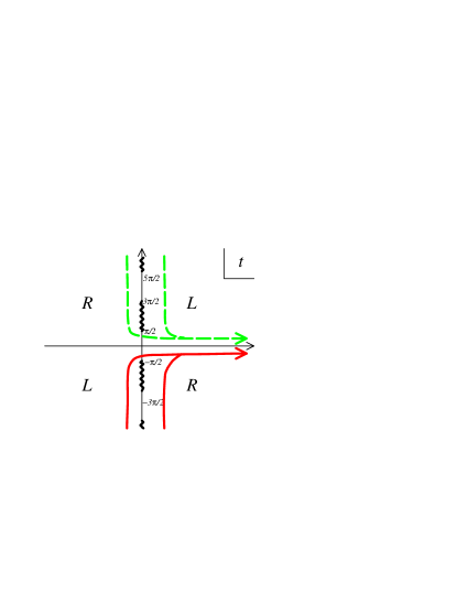
Figure 4: ‘future Hartle-Hawking contour’ : the red (green broken) line is the contour ${\cal C}^{+}_{\mbox{\scriptsize future}}$ for $\omega>0$ (${\cal C}^{-}_{\mbox{\scriptsize future}}$ for $\omega<0$). The ‘$L$’ (‘$R$’) contour should be used if calculating the overlap with $L^{p}_{\omega}(\rho,t)$ ($R^{p}_{\omega}(\rho,t)$) for the convergence of integral.

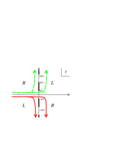
Figure 5: ‘past Hartle-Hawking contour’ : the red (green broken) line is the contour ${\cal C}^{+}_{\mbox{\scriptsize past}}$ for $\omega>0$ (${\cal C}^{-}_{\mbox{\scriptsize past}}$ for $\omega<0$).

One may paraphrase the prescription as follows: choosing the Hartle-Hawking contour ${\cal C}_{\mbox{\scriptsize future}}$, we explicitly obtain

$${}_{HH+,\,\mbox{\scriptsize absorb}}\!{\langle B;\rho_{0},t_{0}|}=\int_{0}^{\infty}\frac{\mbox{d}p}{2\pi}\,\left[\int_{0}^{\infty}\frac{\mbox{d}\omega}{2\pi}\,\Psi_{\mbox{\scriptsize symm}}(\rho_{0},t_{0};p,\omega)+\int_{-\infty}^{0}\frac{\mbox{d}\omega}{2\pi}\,{\cal R}(p,\omega)\Psi^{*}_{\mbox{\scriptsize symm}}(\rho_{0},-t_{0};p,\omega)\right]\,{}^{\widehat{U}}\!{\left\langle\left\langle p,\omega\right|\right.}~{},$$

(116)

where $\Psi_{\mbox{\scriptsize symm}}(\rho_{0},t_{0};p,\omega)$ is defined in (73). In fact, by taking ${\cal C}_{\mbox{\scriptsize future}}$, we are only left with the $L^{p}_{\omega}$ ($R^{p}_{\omega}$)-part of the one-point function for the $\omega>0$ ($\omega<0$) sector. See the figure 4. This boundary wave function is formally regarded as the limit of (67) under $t_{0}\,\rightarrow\,-\infty$, $\rho_{0}\,\rightarrow\,+\infty$ while keeping $|\rho_{0}|/|t_{0}|$ finite. Note that the second (first) term $\propto e^{ip\rho_{0}-i\omega t_{0}}$ ($\propto e^{-ip\rho_{0}-i\omega t_{0}}$) in (67) oscillates very rapidly in this limit for $\omega>0$ ($\omega<0$) and hence drops off. The limit just means that the D0-brane moving along the trajectory (32) is coming from the past infinity $({\cal I}^{-})$, and falling into the future horizon (${\cal H}^{+}$). Everything is supposed to be localized over the classical trajectory in this case.

Adopting the past Hartle-Hawking contour ${\cal C}_{\mbox{\scriptsize past}}$ for the boundary state of emitted D0-brane (69) is completely parallel. We take the time-reversal of the above:

$${}_{HH-,\,\mbox{\scriptsize emit}}\!{\langle B;\rho_{0},t_{0}|}=\int_{0}^{\infty}\frac{\mbox{d}p}{2\pi}\left[\int_{0}^{\infty}\frac{\mbox{d}\omega}{2\pi}\,\Psi^{*}_{\mbox{\scriptsize symm}}(\rho_{0},-t_{0};p,\omega)+\int_{-\infty}^{0}\frac{\mbox{d}\omega}{2\pi}\,{\cal R}^{*}(p,\omega)\Psi_{\mbox{\scriptsize symm}}(\rho_{0},t_{0};p,\omega)\right]{}^{\widehat{V}}\!{\left\langle\left\langle p,\omega\right|\right.}~{},$$

(117)

which is regarded as the $t_{0}\,\rightarrow\,+\infty$, $\rho_{0}\,\rightarrow\,+\infty$ limit of (69). It describes the trajectory of D0-brane emitted from the past horizon ${\cal H}^{-}$ and escaping to the future infinity ${\cal I}^{+}$.

Let us turn to the ‘symmetric’ D0-brane (73). Naively, it appears that the prescription is that

$${}_{HH+,\,\mbox{\scriptsize symm}}\!{\langle B;\rho_{0},t_{0}|}^{\prime}=\int_{0}^{\infty}\frac{\mbox{d}p}{2\pi}\left[\int_{0}^{\infty}\frac{\mbox{d}\omega}{2\pi}\,2\Psi_{\mbox{\scriptsize symm}}(\rho_{0},t_{0};p,\omega)\,{}^{L}\!{\left\langle\left\langle p,\omega\right|\right.}+\int_{-\infty}^{0}\frac{d\omega}{2\pi}\,2\Psi^{*}_{\mbox{\scriptsize symm}}(\rho_{0},-t_{0};p,\omega){}^{R}\!{\left\langle\left\langle p,\omega\right|\right.}\right]$$

(118)

for the future Hartle-Hawking contour ${\cal C}_{\mbox{\scriptsize future}}$, and

$${}_{HH-,\,\mbox{\scriptsize symm}}\!{\langle B;\rho_{0},t_{0}|}^{\prime}=\int_{0}^{\infty}\frac{\mbox{d}p}{2\pi}\left[\int_{0}^{\infty}\frac{\mbox{d}\omega}{2\pi}\,2\Psi^{*}_{\mbox{\scriptsize symm}}(\rho_{0},-t_{0};p,\omega){}^{R}\!{\left\langle\left\langle p,\omega\right|\right.}+\int_{-\infty}^{0}\frac{d\omega}{2\pi}2\Psi_{\mbox{\scriptsize symm}}(\rho_{0},t_{0};p,\omega){}^{L}\!{\left\langle\left\langle p,\omega\right|\right.}\right]$$

(119)

for the past Hartle-Hawking contour ${\cal C}_{\mbox{\scriptsize past}}$. However, this cannot be the whole story. The existence of Euclidean part of the Hartle-Hawking path-integral enforces the boundary states to be expanded by the basis smoothly connected to the Euclidean ones, while ${|L^{p}_{\omega}\rangle}$, ${|R^{p}_{\omega}\rangle}$ do not possess such a property. Consequently, to achieve the correct Hartle-Hawking states, we ought to make further the projection to ${\cal H}^{U}$, ($\widehat{{\cal H}^{U}}$) for the contour ${\cal C}_{\mbox{\scriptsize future}}$, and to ${\cal H}^{V}$, ($\widehat{{\cal H}^{V}}$) for ${\cal C}_{\mbox{\scriptsize past}}$. We thus obtain as the correct Hartle-Hawking states:

$${}_{HH+,\,\mbox{\scriptsize symm}}\!{\langle B;\rho_{0},t_{0}|}={}_{HH+,\,\mbox{\scriptsize symm}}\!{\langle B;\rho_{0},t_{0}|}^{\prime}\widehat{P_{U}}\equiv{}_{HH+,\,\mbox{\scriptsize absorb}}\!{\langle B;\rho_{0},t_{0}|}~{},$$

$${}_{HH-,\,\mbox{\scriptsize symm}}\!{\langle B;\rho_{0},t_{0}|}={}_{HH-,\,\mbox{\scriptsize symm}}\!{\langle B;\rho_{0},t_{0}|}^{\prime}\widehat{P_{V}}\equiv{}_{HH-,\,\mbox{\scriptsize emitted}}\!{\langle B;\rho_{0},t_{0}|}~{},$$ (120)

where the right-hand sides are already given in (116), (117).

Remarkably, this feature resembles much that of the S-branes discussed in [36]. Namely, it was shown there that

$$\mbox{half S-brane}~{}\cong~{}\mbox{full S-brane with the Hartle-Hawking contour}~{}.$$ (121)

In our case, (73) corresponds to the full S-brane, while the Hartle-Hawking state (116) ((117)) is identifiable as the analogue of the half S-brane describing unstable D-brane decay (creation) process. The equalities (120) suggest that we have roughly identical relation to (121).

Notice that the parameters $\rho_{0}$, $t_{0}$ appear just as phase factors of boundary wave functions in (116), (117) contrary to (67), (69). Namely, the choice of parameters $\rho_{0}$, $t_{0}$ does not cause any physical difference for the Hartle-Hawking type states : They all can be regarded as describing the D0-brane moving from ${\cal I}^{-}$ to ${\cal H}^{+}$ (from ${\cal H}^{-}$ to ${\cal I}^{+}$) for (116) (for (117)) irrespective of $\rho_{0}$, $t_{0}$. These two parameters merely parameterize displacing the trajectory in two-dimensional black hole background. Similar feature comes about for the full S-brane with Hartle-Hawking contour as well: It is equivalent to the half S-brane not depending on any shift of the origin (the point connecting the real and imaginary times).

Finally, we remark a comment from the viewpoints of boundary conformal field theory: in contrast to the original ones (67), (69) and (73), the Hartle-Hawking boundary states (120) (or equivalently (116), (117)) are not compatible with the reflection relations. One may regard the boundary states (67) and (69) as the ‘completions’ of the Hartle-Hawking states (120) so that they satisfy the reflection relations.

Note Added : After this work was published, the work [56] was brought to our attention. However, the work [56] claimed results discrepant with ours concerning treatment of spectral amplitudes and the closed string radiations. We made in another publication [57] further investigation from the open string channel. The result of [57] completely supports the result given in this work, and clarifies where the errors originate in the work [56].

Appendix A   Useful Formulae

$$\int_{-\frac{\pi}{2}}^{\frac{\pi}{2}}(2\cos\theta)^{a-1}e^{ib\theta}\mbox{d}\theta=\pi\frac{\Gamma(a)}{\Gamma\left(\frac{1}{2}+\frac{a+b}{2}\right)\Gamma\left(\frac{1}{2}+\frac{a-b}{2}\right)}~{},~{}~{}~{}(\mbox{Re}\,a>0~{},~{}~{}\left|\mbox{Re}\,b\right|<\mbox{Re}\,a+1)~{},$$ (A.1)

$$\int_{-\infty}^{\infty}(2\cosh t)^{a-1}e^{ibt}\mbox{d}t=\frac{1}{2}B\left(\frac{1}{2}-\frac{a+ib}{2},\frac{1}{2}-\frac{a-ib}{2}\right)\equiv\frac{1}{2}\frac{\Gamma\left(\frac{1}{2}-\frac{a+ib}{2}\right)\Gamma\left(\frac{1}{2}-\frac{a-ib}{2}\right)}{\Gamma(1-a)}~{},$$

$$\hskip 284.52756pt(\mbox{Re}\,a<1~{},~{}~{}\left|\mbox{Im}\,b\right|<1-\mbox{Re}\,a)~{}.$$ (A.2)

The integral (A.2) follows from the more general formula:

$$\int_{0}^{\infty}\frac{\cosh(2at)}{\cosh^{2\beta}(pt)}\mbox{d}t=4^{\beta-1}p^{-1}B\left(\beta+\frac{a}{p},\beta-\frac{a}{p}\right)~{},~{}~{}~{}(p>0,~{}~{}\mbox{Re}\,\left(\beta\pm\frac{a}{p}\right)>0)~{},$$ (A.3)

given in [58]. It is also derivable from (A.1) by contour deformation, as was shown in [13].

Appendix B   Proof of (29)

Here we would like to evaluate explicitly the integral (29) for any $\rho_{0}$ (strictly speaking, we need to assume $\sinh\rho_{0}>1$). We begin with series expansion of the hypergeometric function in $\phi^{p}_{n}(\rho,\theta)$:

$$F\left(\frac{1}{2}+\frac{ip+n}{2},\frac{1}{2}+\frac{ip-n}{2};ip+1;-\frac{\cos^{2}\theta}{\sinh^{2}\rho_{0}}\right)$$

$$=\sum_{\ell=0}^{\infty}\frac{\Gamma(ip+1)}{\Gamma(\frac{1}{2}+\frac{ip+n}{2})\Gamma(\frac{1}{2}+\frac{ip-n}{2})}\frac{\Gamma(\frac{1}{2}+\frac{ip+n}{2}+\ell)\Gamma(\frac{1}{2}+\frac{ip-n}{2}+\ell)}{\Gamma(ip+1+\ell)}\frac{(-1)^{\ell}}{\ell!}\left(\frac{\cos\theta}{\sinh\rho_{0}}\right)^{2\ell}\ .$$ (B.1)

Using the formula (A.1), we can perform, in the $\ell$-th sector, the integral (29) as

$$\Psi_{\ell}=g(\ell)\int_{-\frac{\pi}{2}}^{\frac{\pi}{2}}\mbox{d}\theta\,e^{in\theta}(\cos\theta)^{ip-1+2\ell}=\frac{g(\ell)}{2^{ip-1+2\ell}}\cdot\frac{\pi\Gamma(ip-1+2\ell+1)}{\Gamma(\frac{1}{2}+\ell+\frac{ip+n}{2})\Gamma(\frac{1}{2}+\ell+\frac{ip-n}{2})}\ ,$$

where $g(\ell)$ refers to

$$g(\ell)=\frac{(-1)^{\ell}}{\ell!}(\sinh\rho_{0})^{-ip-2\ell}\frac{\Gamma(ip+1)}{\Gamma(\frac{1}{2}+\frac{ip+n}{2})\Gamma(\frac{1}{2}+\frac{ip-n}{2})}\frac{\Gamma(\frac{1}{2}+\frac{ip+n}{2}+\ell)\Gamma(\frac{1}{2}+\frac{ip-n}{2}+\ell)}{\Gamma(ip+1+\ell)}\ .$$ (B.2)

Then the total integral (29) is

$$\sum_{\ell=0}^{\infty}\Psi_{\ell}=\frac{\pi}{2^{ip-1}(\sinh\rho_{0})^{ip}}\frac{\Gamma(ip+1)}{\Gamma(\frac{1}{2}+\frac{ip+n}{2})\Gamma(\frac{1}{2}+\frac{ip-n}{2})}\sum_{\ell=0}^{\infty}\frac{(-1)^{\ell}}{\ell!}\frac{1}{2^{2\ell}(\sinh\rho_{0})^{2\ell}}\frac{\Gamma(ip+2\ell)}{\Gamma(ip+1+\ell)}\ .$$ (B.3)

We can rewrite the summation into a hypergeometric function by using

$$\Gamma(ip+2\ell)=\frac{2^{ip-1+2\ell}}{\sqrt{\pi}}\Gamma\left(\frac{ip}{2}+\ell\right)\Gamma\left(\frac{1}{2}+\frac{ip}{2}+\ell\right)~{}.$$ (B.4)

and then obtain

$$\sum_{\ell=0}^{\infty}\Psi_{\ell}=\frac{\sqrt{\pi}}{(\sinh\rho_{0})^{ip}}\frac{\Gamma(\frac{ip}{2})\Gamma(\frac{1}{2}+\frac{ip}{2})}{\Gamma(\frac{1}{2}+\frac{ip+n}{2})\Gamma(\frac{1}{2}+\frac{ip-n}{2})}F\left(\frac{ip}{2},\frac{1}{2}+\frac{ip}{2};ip+1;-\frac{1}{\sinh^{2}\rho_{0}}\right)\ .$$ (B.5)

Making use of the formula

$$F\left(2\alpha,2\beta;\alpha+\beta+\frac{1}{2};z\right)=F\left(\alpha,\beta;\alpha+\beta+\frac{1}{2};4z(1-z)\right)\ .$$ (B.6)

$$\hskip 142.26378pt|z|<\frac{1}{2},\quad|z(1-z)|<\frac{1}{4}~{}$$

we find that

$$\sum_{\ell=0}^{\infty}\Psi_{\ell}=\frac{\sqrt{\pi}}{(\sinh\rho_{0})^{ip}}\frac{\Gamma(\frac{ip}{2})\Gamma(\frac{1}{2}+\frac{ip}{2})}{\Gamma(\frac{1}{2}+\frac{ip+n}{2})\Gamma(\frac{1}{2}+\frac{ip-n}{2})}F\left(ip,ip+1;ip+1;\frac{1}{2}-\frac{\cosh\rho_{0}}{2\sinh\rho_{0}}\right)\ .$$ (B.7)

Note that the second and third arguments of the hypergeometric function are the same. The function is thus simplified as

$$F\left(ip,ip+1;ip+1;\frac{1}{2}-\frac{\cosh\rho_{0}}{2\sinh\rho_{0}}\right)=\left(\frac{\sinh\rho_{0}+\cosh\rho_{0}}{2\sinh\rho_{0}}\right)^{-ip}=\left(2e^{-\rho_{0}}\sinh\rho_{0}\right)^{ip}~{},$$ (B.8)

because of the relation

$$(1-z)^{\alpha}=F(-\alpha,\beta;\beta;z)~{}.$$ (B.9)

In this way, we finally obtain

$$\sum_{\ell=0}^{\infty}\Psi_{\ell}=\sqrt{\pi}e^{-ip\rho_{0}}2^{ip}\frac{\Gamma(\frac{ip}{2})\Gamma(\frac{1}{2}+\frac{ip}{2})}{\Gamma(\frac{1}{2}+\frac{ip+n}{2})\Gamma(\frac{1}{2}+\frac{ip-n}{2})}=\frac{2\pi\,\Gamma(ip)}{\Gamma(\frac{1}{2}+\frac{ip+n}{2})\Gamma(\frac{1}{2}+\frac{ip-n}{2})}e^{-ip\rho_{0}}~{},$$ (B.10)

and this is the desired formula.

References

- [1] A. Sen, JHEP 0204, 048 (2002) [arXiv:hep-th/0203211]; JHEP 0207, 065 (2002) [arXiv:hep-th/0203265]; Mod. Phys. Lett. A 17, 1797 (2002) [arXiv:hep-th/0204143].
- [2] E. Witten, Phys. Rev. D44 (1991) 314; G S. Elitzur, A. Forge and E. Rabinovici, Nucl. Phys. B359 (1991) 581; Mandal, A. Sengupta and S. Wadia, Mod. Phys. Lett. A6 (1991) 1685; I. Bars and D. Nemeschansky, Nucl. Phys. B348 (1991) 89.
- [3] R. Dijkgraaf, H. Verlinde and E. Verlinde, Nucl. Phys. B 371, 269 (1992).
- [4] G. T. Horowitz and A. Strominger, Nucl. Phys. B 360, 197 (1991).
- [5] S. J. Rey, Phys. Rev. D 43, 526 (1991); ibid. ”Axionic String Instantons and Their Low-Energy Implications”, UCSB-TH-89/49, in the proceedings of the ”Workshop on Superstrings and Particle Theory” pp. 291-300 (World Scientific Pub., 1989).
- [6] C. G. . Callan, J. A. Harvey and A. Strominger, Nucl. Phys. B 359, 611 (1991); S. J. Rey, ”On String Theory and Axionic Strings and Instantons”, SLAC-PUB-5659, in the proceedings of ”Particle and Fields ’91 Conference” pp. 876-881 (American Physical Society, 1991).
- [7] D. Kutasov, arXiv:hep-th/0405058.
- [8] D. Kutasov, arXiv:hep-th/0408073.
- [9] A. Strominger, arXiv:hep-th/0209090.
- [10] F. Larsen, A. Naqvi and S. Terashima, JHEP 0302, 039 (2003) [arXiv:hep-th/0212248].
- [11] H. Yavartanoo, arXiv:hep-th/0407079; K. L. Panigrahi, Phys. Lett. B 601, 64 (2004) [arXiv:hep-th/0407134]; A. Ghodsi and A. E. Mosaffa, Nucl. Phys. B 714, 30 (2005) [arXiv:hep-th/0408015]; J. Kluson, JHEP 0411, 013 (2004) [arXiv:hep-th/0409298]; arXiv:hep-th/0501010; B. Chen and B. Sun, arXiv:hep-th/0501176; D. Bak, S. J. Rey and H. U. Yee, JHEP 0412, 008 (2004) [arXiv:hep-th/0411099]; S. Thomas and J. Ward, JHEP 0502, 015 (2005) [arXiv:hep-th/0411130]; arXiv:hep-th/0501192, arXiv:hep-th/0502228; arXiv:hep-th/0504226; W. H. Huang, JHEP 0502, 061 (2005) [arXiv:hep-th/0502023]; J. Kluson and K. L. Panigrahi, arXiv:hep-th/0506012.
- [12] I. Bars and K. Sfetsos, Phys. Rev. D 46, 4495 (1992) [arXiv:hep-th/9205037]; I. Bars and J. Schulze, Phys. Rev. D 51, 1854 (1995) [arXiv:hep-th/9405156].
- [13] Y. Nakayama, Y. Sugawara and H. Takayanagi, JHEP 0407, 020 (2004) [arXiv:hep-th/0406173].
- [14] Y. Nakayama, K. L. Panigrahi, S. J. Rey and H. Takayanagi, JHEP 0501, 052 (2005) [arXiv:hep-th/0412038].
- [15] D. A. Sahakyan, JHEP 0410, 008 (2004) [arXiv:hep-th/0408070].
- [16] B. Chen, M. Li and B. Sun, JHEP 0412, 057 (2004) [arXiv:hep-th/0412022];
- [17] J. M. Lapan and W. Li, arXiv:hep-th/0501054.
- [18] J. M. Maldacena and A. Strominger, JHEP 9712, 008 (1997) [arXiv:hep-th/9710014];
- [19] S. Ribault and V. Schomerus, JHEP 0402, 019 (2004) [arXiv:hep-th/0310024].
- [20] J. L. Karczmarek, J. Maldacena and A. Strominger, arXiv:hep-th/0411174.
- [21] A. Giveon, D. Kutasov, E. Rabinovici and A. Sever, arXiv:hep-th/0503121.
- [22] J. Maldacena, arXiv:hep-th/0503112.
- [23] J. Teschner, Nucl. Phys. B 546, 390 (1999) [arXiv:hep-th/9712256]; Nucl. Phys. B 571, 555 (2000) [arXiv:hep-th/9906215].
- [24] A. Giveon and D. Kutasov, JHEP 9910, 034 (1999) [arXiv:hep-th/9909110]; A. Giveon and D. Kutasov, JHEP 0001, 023 (2000) [arXiv:hep-th/9911039].
- [25] C. Bachas and M. Petropoulos, JHEP 0102, 025 (2001) [arXiv:hep-th/0012234].
- [26] B. Ponsot, V. Schomerus and J. Teschner, JHEP 0202, 016 (2002) [arXiv:hep-th/0112198]; A. Giveon, D. Kutasov and A. Schwimmer, Nucl. Phys. B 615, 133 (2001) [arXiv:hep-th/0106005]; P. Lee, H. Ooguri and J. W. Park, Nucl. Phys. B 632, 283 (2002) [arXiv:hep-th/0112188].
- [27] S. L. Lukyanov, E. S. Vitchev and A. B. Zamolodchikov, Nucl. Phys. B 683, 423 (2004) [arXiv:hep-th/0312168].
- [28] T. Eguchi and Y. Sugawara, JHEP 0401, 025 (2004) [arXiv:hep-th/0311141].
- [29] C. Ahn, M. Stanishkov and M. Yamamoto, Nucl. Phys. B 683, 177 (2004) [arXiv:hep-th/0311169].
- [30] D. Israel, A. Pakman and J. Troost, Nucl. Phys. B 710, 529 (2005) [arXiv:hep-th/0405259].
- [31] A. Fotopoulos, V. Niarchos and N. Prezas, Nucl. Phys. B 710, 309 (2005) [arXiv:hep-th/0406017].
- [32] Y. Nakayama, Int. J. Mod. Phys. A 19, 2771 (2004) [arXiv:hep-th/0402009].
- [33] K. P. Yogendran, JHEP 0501, 036 (2005) [arXiv:hep-th/0408114].
- [34] M. Gutperle and A. Strominger, JHEP 0204, 018 (2002) [arXiv:hep-th/0202210].
- [35] C. G. . Callan and J. M. Maldacena, Nucl. Phys. B 472, 591 (1996) [arXiv:hep-th/9602043]; S. R. Das and S. D. Mathur, Nucl. Phys. B 478, 561 (1996) [arXiv:hep-th/9606185].
- [36] N. Lambert, H. Liu and J. Maldacena, arXiv:hep-th/0303139.
- [37] J. L. Karczmarek, H. Liu, J. Maldacena and A. Strominger, JHEP 0311, 042 (2003) [arXiv:hep-th/0306132].
- [38] G. ’t Hooft, Print-87-0775 (UTRECHT) Lectures given at Cargese Summer Inst. on Nonperturbative Quantum Field Theory, Cargese, France, Jul 16-30, 1987; C. F. E. Holzhey and F. Wilczek, Nucl. Phys. B 380, 447 (1992) [arXiv:hep-th/9202014]; G. T. Horowitz and J. Polchinski, Phys. Rev. D 55, 6189 (1997) [arXiv:hep-th/9612146].
- [39] A. Giveon, A. Konechny, A. Pakman and A. Sever, JHEP 0310, 025 (2003) [arXiv:hep-th/0309056].
- [40] D. Kutasov and N. Seiberg, Nucl. Phys. B 358, 600 (1991).
- [41] Y. Sugawara, Nucl. Phys. B 650, 75 (2003) [arXiv:hep-th/0209145], JHEP 0308, 008 (2003) [arXiv:hep-th/0307034].
- [42] J. Polchinski, Commun. Math. Phys. 104, 37 (1986); B. Sathiapalan, Phys. Rev. D 35, 3277 (1987); Y. I. Kogan, JETP Lett. 45, 709 (1987) [Pisma Zh. Eksp. Teor. Fiz. 45, 556 (1987)]; K. H. O’Brien and C. I. Tan, Phys. Rev. D 36, 1184 (1987); J. J. Atick and E. Witten, Nucl. Phys. B 310, 291 (1988).
- [43] D. Kutasov and N. Seiberg, Phys. Lett. B 251, 67 (1990).
- [44] V. Fateev, A. B. Zamolodchikov and Al. B. Zamolodchikov, unpublished; V. Kazakov, I. K. Kostov and D. Kutasov, Nucl. Phys. B 622, 141 (2002) [arXiv:hep-th/0101011].
- [45] K. Hori and A. Kapustin, JHEP 0108, 045 (2001) [arXiv:hep-th/0104202].
- [46] J. J. Friess and H. Verlinde, arXiv:hep-th/0411100.
- [47] I. R. Klebanov, J. Maldacena and N. Seiberg, JHEP 0307, 045 (2003) [arXiv:hep-th/0305159].
- [48] A. Giveon, D. Kutasov and O. Pelc, JHEP 9910, 035 (1999) [arXiv:hep-th/9907178].
- [49] O. Aharony, A. Giveon and D. Kutasov, Nucl. Phys. B 691, 3 (2004) [arXiv:hep-th/0404016].
- [50] T. Eguchi and Y. Sugawara, JHEP 0405, 014 (2004) [arXiv:hep-th/0403193].
- [51] T. Eguchi and Y. Sugawara, JHEP 0501, 027 (2005) [arXiv:hep-th/0411041].
- [52] O. Aharony, M. Berkooz, D. Kutasov and N. Seiberg, JHEP 9810, 004 (1998) [arXiv:hep-th/9808149].
- [53] T. Harmark and N. A. Obers, Phys. Lett. B 485, 285 (2000) [arXiv:hep-th/0005021].
- [54] M. Berkooz and M. Rozali, JHEP 0005, 040 (2000) [arXiv:hep-th/0005047].
- [55] D. Kutasov and D. A. Sahakyan, JHEP 0102, 021 (2001) [arXiv:hep-th/0012258].
- [56] K. Okuyama and M. Rozali, arXiv:hep-th/0602060. JHEP 0603, 071 (2006) [arXiv:hep-th/0602060].
- [57] Y. Nakayama, S. J. Rey and Y. Sugawara, [arXiv:hep-th/0605013].
- [58] H. Bateman, “Higher Transcendental Functions,” Vol. 1. McGRAW-Hill BOOK COMPANY, INC. (1953)