Thermodynamics of Asymptotically Flat Charged Black Holes in Third Order Lovelock Gravity

Abstract

We present a new class of asymptotically flat charge static solutions in third order Lovelock gravity. These solutions present black hole solutions with two inner and outer event horizons, extreme black holes or naked singularities provided the parameters of the solutions are chosen suitable. We find that the uncharged asymptotically flat solutions can present black hole with two inner and outer horizons. This kind of solution does not exist in Einstein or Gauss-Bonnet gravity, and it is a special effect in third order Lovelock gravity. We compute temperature, entropy, charge, electric potential and mass of the black hole solutions, and find that these quantities satisfy the first law of thermodynamics. We also perform a stability analysis by computing the determinant of Hessian matrix of the mass with respect to its thermodynamic variables in both the canonical and the grand-canonical ensembles, and show that there exists only an intermediate stable phase.

I Introduction

Both string theory as well as brane world cosmology assume that spacetime possesses more than four dimensions. In string theory, extra dimensions were promoted from an interesting curiosity to a theoretical necessity since superstring theory requires a ten-dimensional spacetime to be consistent from the quantum point of view, while in the brane world cosmology (which is also consistent with string theory) the matter and gauge interaction are localized on a 3-brane, embedded into a higher dimensional spacetime and gravity propagates in the whole of spacetime. This underscores the need to consider gravity in higher dimensions. In this context one may use another consistent theory of gravity in any dimension with a more general action. This action may be written, for example, through the use of string theory. The effect of string theory on classical gravitational physics is usually investigated by means of a low energy effective action which describes gravity at the classical level Wit1 . This effective action consists of the Einstein-Hilbert action plus curvature-squared terms and higher powers as well, and in general give rise to fourth order field equations and bring in ghosts. However, if the effective action contains the higher powers of curvature in particular combinations, then only second order field equations are produced and consequently no ghosts arise Zw . The effective action obtained by this argument is precisely of the form proposed by Lovelock Lov :

$$I_{G}=\int d^{d}x\sqrt{-g}\sum_{k=0}^{[d/2]}\alpha_{k}\mathcal{L}_{k}$$ (1)

where $[z]$ denotes integer part of $z$, $\alpha_{k}$ is an arbitrary constant and $\mathcal{L}_{k}$ is the Euler density of a $2k$-dimensional manifold,

$$\mathcal{L}_{k}=\frac{1}{2^{k}}\delta_{\rho_{1}\sigma_{1}\cdots\rho_{k}\sigma_{k}}^{\mu_{1}\nu_{1}\cdots\mu_{k}\nu_{k}}R_{\mu_{1}\nu_{1}}^{\phantom{\mu_{1}\nu_{1}}{\rho_{1}\sigma_{1}}}\cdots R_{\mu_{k}\nu_{k}}^{\phantom{\mu_{k}\nu_{k}}{\rho_{k}\sigma_{k}}}$$ (2)

In Eq. (2) $\delta_{\rho_{1}\sigma_{1}\cdots\rho_{k}\sigma_{k}}^{\mu_{1}\nu_{1}\cdots\mu_{k}\nu_{k}}$ is the generalized totally anti-symmetric Kronecker delta and $R_{\mu\nu}^{\phantom{\mu\nu}{\rho\sigma}}$ is the Riemann tensor. It is worthwhile to mention that in $d$ dimensions, all terms for which $k>[d/2]$ are identically equal to zero, and the term $k=d/2$ is a topological term. So, only terms for which $k<d/2$ are contributing to the field equations.

In this paper we want to restrict ourself to the first four terms of Lovelock gravity. The first term is the cosmological term which we ignore it in the investigation of the properties and thermodynamics of the solutions. The second term is the Einstein term, and the third and fourth terms are the second order Lovelock (Gauss-Bonnet) and third order Lovelock terms respectively. From a geometric point of view, the combination of these terms in seven-dimensional spacetimes, is the most general Lagrangian producing second order field equations, as in the four-dimensional gravity which the Einstein-Hilbert action is the most general Lagrangian producing second order field equations. Here, we will obtain asymptotically flat solutions of third order Lovelock gravity and investigate their thermodynamics.

Indeed, it is interesting to explore black holes in generalized gravity theories in order to discover which properties are peculiar to Einstein’s gravity, and which are robust features of all generally covariant theories of gravity. Due to the nonlinearity of the field equations, it is very difficult to find out nontrivial exact analytical solutions of Einstein’s equation with the higher curvature terms. In most cases, one has to adopt some approximation methods or find solutions numerically. However, exact static spherically symmetric black hole solutions of the Gauss-Bonnet gravity have been found in Ref. Des ; Whe , and of the Einstein-Maxwell-Gauss-Bonnet and Einstein-Born-Infeld-Gauss-Bonnet models in Refs. Wil1 ; Wil2 . Black hole solutions with nontrivial topology in this theory have been also studied in Refs. Cai ; Ish . The thermodynamics of the uncharged static spherically black hole solutions has been considered in MS and of charged solutions in Wil2 ; Odin . All of these known solutions in Gauss-Bonnet gravity are static. Recently one of us has introduced two new classes of rotating solutions of second order Lovelock gravity and investigate their thermodynamics Deh1 .

Also the static spherically symmetric solutions of the dimensionality continued gravity have been explored in Ref. Zan , while black hole solutions with nontrivial topology in this theory have been studied in Ref. Aros . The thermodynamics of these solutions have been investigated in Refs. Mun ; Chr ; Clu . Up to our knowledge, no asymptotically flat solution for Lovelock gravity higher than second order (Gauss-Bonnet) has been obtained till now with two or more fundamental constants. Indeed, the asymptotically flat solution of Ref. Chr has only one fundamental constant which is the gravitational constant $G$. In this paper we want to find new static solutions of third order Lovelock gravity which are asymptotically flat and contain two and three fundamental constants and investigate their thermodynamics. As we will show later, these asymptotically flat solutions have some properties which do not occur in Einstein or Gauss-Bonnet gravity.

The outline of our paper is as follows. We give a brief review of the field equations of third order Lovelock gravity in Sec. II. In Sec. III, we present the static solutions of third order Lovelock gravity in the presence of electromagnetic field with special values of $\alpha_{2}$ and $\alpha_{3}$, and investigate their properties. In Sec. IV we obtain mass, entropy, temperature, charge, and electric potential of the $d$-dimensional black hole solutions and show that these quantities satisfy the first law of thermodynamics. We also perform a local stability analysis of the black holes in the canonical and grand canonical ensembles. In Sec. V, we introduce the general asymptotically flat solutions with three fundamental constants and investigate their thermodynamics. We finish our paper with some concluding remarks.

II Field equations

The main fundamental assumptions in standard general relativity are the requirements of general covariance and that the field equations for the metric be second order. Based on the same principles, the Lovelock Lagrangian is the most general Lagrangian in classical gravity which produces second order field equations for the metric. The action of third order Lovelock gravity in the presence of electromagnetic field may be written as

$$I=\int d^{d}x\sqrt{-g}\left(-2\Lambda+\mathcal{L}_{1}+\alpha_{2}\mathcal{L}_{2}+\alpha_{3}\mathcal{L}_{3}-F_{\mu\nu}F^{\mu\nu}\right)$$ (3)

where $\Lambda$ is the cosmological constant, $\alpha_{2}$ and $\alpha_{3}$ are Gauss-Bonnet and third order lovelock coefficients, $\mathcal{L}_{1}=R$ is just the Einstein-Hilbert Lagrangian, $\mathcal{L}_{2}=R_{\mu\nu\gamma\delta}R^{\mu\nu\gamma\delta}-4R_{\mu\nu}R^{\mu\nu}+R^{2}$ is the Gauss-Bonnet Lagrangian, and

$$\mathcal{L}_{3} = 2R^{\mu\nu\sigma\kappa}R_{\sigma\kappa\rho\tau}R_{\phantom{\rho\tau}{\mu\nu}}^{\rho\tau}+8R_{\phantom{\mu\nu}{\sigma\rho}}^{\mu\nu}R_{\phantom{\sigma\kappa}{\nu\tau}}^{\sigma\kappa}R_{\phantom{\rho\tau}{\mu\kappa}}^{\rho\tau}+24R^{\mu\nu\sigma\kappa}R_{\sigma\kappa\nu\rho}R_{\phantom{\rho}{\mu}}^{\rho}$$ (4)

$$+3RR^{\mu\nu\sigma\kappa}R_{\sigma\kappa\mu\nu}+24R^{\mu\nu\sigma\kappa}R_{\sigma\mu}R_{\kappa\nu}+16R^{\mu\nu}R_{\nu\sigma}R_{\phantom{\sigma}{\mu}}^{\sigma}-12RR^{\mu\nu}R_{\mu\nu}+R^{3}$$

is the third order Lovelock Lagrangian. In Eq. (3) $F_{\mu\nu}=\partial_{\mu}A_{\nu}-\partial_{\nu}A_{\mu}$ is electromagnetic tensor field and $A_{\mu}$ is the vector potential.

Since in Lovelock gravity, only terms for which $k<d/2$ are contributing to the field equations and we want to consider the third order lovelock gravity, therefore we consider the $d$-dimensional spacetimes with $d\geq 7$. Varying the action with respect to the metric tensor $g_{\mu\nu}$ and electromagnetic tensor field $F_{\mu\nu}$ the equations of gravitation and electromagnetic fields are obtained as:

$$G_{\mu\nu}^{(1)}+\Lambda g_{\mu\nu}+\alpha_{2}G_{\mu\nu}^{(2)}+\alpha_{3}G_{\mu\nu}^{(3)}=T_{\mu\nu}$$ (5)

$$\nabla_{\nu}F^{\mu\nu}=0$$ (6)

where $T_{\mu\nu}=2F_{\phantom{\lambda}{\mu}}^{\rho}F_{\rho\nu}-\frac{1}{2}F_{\rho\sigma}F^{\rho\sigma}g_{\mu\nu}$ is the energy-momentum tensor of electromagnetic field, $G_{\mu\nu}^{(1)}$ is just the Einstein tensor, and $G_{\mu\nu}^{(2)}$ and $G_{\mu\nu}^{(3)}$ are given as Hoi :

$$G_{\mu\nu}^{(2)} = 2(-R_{\mu\sigma\kappa\tau}R_{\phantom{\kappa\tau\sigma}{\nu}}^{\kappa\tau\sigma}-2R_{\mu\rho\nu\sigma}R^{\rho\sigma}-2R_{\mu\sigma}R_{\phantom{\sigma}\nu}^{\sigma}+RR_{\mu\nu})-\frac{1}{2}\mathcal{L}_{2}g_{\mu\nu}$$

$$G_{\mu\nu}^{(3)} = -3(4R^{\tau\rho\sigma\kappa}R_{\sigma\kappa\lambda\rho}R_{\phantom{\lambda}{\nu\tau\mu}}^{\lambda}-8R_{\phantom{\tau\rho}{\lambda\sigma}}^{\tau\rho}R_{\phantom{\sigma\kappa}{\tau\mu}}^{\sigma\kappa}R_{\phantom{\lambda}{\nu\rho\kappa}}^{\lambda}+2R_{\nu}^{\phantom{\nu}{\tau\sigma\kappa}}R_{\sigma\kappa\lambda\rho}R_{\phantom{\lambda\rho}{\tau\mu}}^{\lambda\rho}$$

$$-R^{\tau\rho\sigma\kappa}R_{\sigma\kappa\tau\rho}R_{\nu\mu}+8R_{\phantom{\tau}{\nu\sigma\rho}}^{\tau}R_{\phantom{\sigma\kappa}{\tau\mu}}^{\sigma\kappa}R_{\phantom{\rho}\kappa}^{\rho}+8R_{\phantom{\sigma}{\nu\tau\kappa}}^{\sigma}R_{\phantom{\tau\rho}{\sigma\mu}}^{\tau\rho}R_{\phantom{\kappa}{\rho}}^{\kappa}$$

$$+4R_{\nu}^{\phantom{\nu}{\tau\sigma\kappa}}R_{\sigma\kappa\mu\rho}R_{\phantom{\rho}{\tau}}^{\rho}-4R_{\nu}^{\phantom{\nu}{\tau\sigma\kappa}}R_{\sigma\kappa\tau\rho}R_{\phantom{\rho}{\mu}}^{\rho}+4R^{\tau\rho\sigma\kappa}R_{\sigma\kappa\tau\mu}R_{\nu\rho}+2RR_{\nu}^{\phantom{\nu}{\kappa\tau\rho}}R_{\tau\rho\kappa\mu}$$

$$+8R_{\phantom{\tau}{\nu\mu\rho}}^{\tau}R_{\phantom{\rho}{\sigma}}^{\rho}R_{\phantom{\sigma}{\tau}}^{\sigma}-8R_{\phantom{\sigma}{\nu\tau\rho}}^{\sigma}R_{\phantom{\tau}{\sigma}}^{\tau}R_{\mu}^{\rho}-8R_{\phantom{\tau}{\sigma\mu}}^{\tau\rho}R_{\phantom{\sigma}{\tau}}^{\sigma}R_{\nu\rho}-4RR_{\phantom{\tau}{\nu\mu\rho}}^{\tau}R_{\phantom{\rho}\tau}^{\rho}$$

$$+4R^{\tau\rho}R_{\rho\tau}R_{\nu\mu}-8R_{\phantom{\tau}{\nu}}^{\tau}R_{\tau\rho}R_{\phantom{\rho}{\mu}}^{\rho}+4RR_{\nu\rho}R_{\phantom{\rho}{\mu}}^{\rho}-R^{2}R_{\nu\mu})-\frac{1}{2}\mathcal{L}_{3}g_{\mu\nu}$$

III Static Solutions

The metric of $d$-dimensional static spherically symmetric spacetime and the vector potential may be written as:

$$ds^{2} = -f(r)dt^{2}+\frac{dr^{2}}{f(r)}+r^{2}d\Omega^{2}$$

$$A_{\mu} = h(r)\delta_{\mu}^{t}$$ (7)

where $d\Omega^{2}$ is the metric of a $(d-2)$-sphere. The functions $f(r)$ and $h(r)$ may be obtained by solving the field equations (5) and (6).

III.1 Seven-dimensional Solutions

As stated before, the gravitational field equation of third order Lovelock gravity in seven dimensions is the most general second order differential equation which presents the solutions of gravity. Indeed, the solution of third order Lovelock gravity in seven dimensions is the most general solution of gravity, based on the principle of standard general relativity. Therefore, first we obtain the seven-dimensional solutions of third order Lovelock gravity in the presence of electromagnetic field and investigate their properties. Using Eq. (6) one can show that $h(r)=q/(4r^{4})$, where $q$ is an arbitrary real constant which is related to the charge of the solution. To find the function $f(r)$, one may use any components of Eq. (5). The simplest equation is the $rr$-component of these equations which can be written as

$$\left(-3\alpha_{3}(f-1)^{2}+\alpha_{2}(f-1)r^{2}-\frac{r^{4}}{24}\right)r^{5}f^{\prime}+\alpha_{2}r^{6}(f-1)^{2}-\frac{r^{8}}{6}(f-1)-\frac{\Lambda}{60}r^{10}=\frac{q^{2}}{60}$$ (8)

where prime denotes the derivative with respect to $r$. We consider the solutions of Eq. (8) for any arbitrary values of $\alpha_{2}$ and $\alpha_{3}$ in Sec. V. Here, we study the special case of $\alpha_{3}=2{\alpha_{2}}^{2}=\alpha^{2}/72$. Even for this special case, there exist three fundamental constants, $\Lambda$, $G=1$ and $\alpha$ in the solution, while the solution of ref. Chr has two fundamental constants. As we will see below this solution has some properties which will not happen in the Gauss-Bonnet gravity with three fundamental constants. The real solution of Eq. (8) with the above values of $\alpha_{2}$ and $\alpha_{3}$ is

$$f(r)=1+{\frac{{r}^{2}}{\alpha}}\left\{1-\left({1+\frac{\Lambda\alpha}{5}+\frac{3\alpha m}{5r^{6}}-\frac{3\alpha{q}^{2}}{10r^{10}}}\right)^{1/3}\right\}$$ (9)

In the above equations $m$ is an integration constant which is related to the mass of the solution. Unlike the solutions in Gauss-Bonnet gravity which have two branches, here the solution (9) has only one branch. Indeed, Eq. (8) with the above $\alpha$’s has the real solution (9) and two complex solutions which are the complex conjugate of each other. This feature is the same as the asymptotically anti-de Sitter (AdS) solution of Ref. Chr which has a unique anti de Sitter vacuum.

In order to study the general structure of this solution, we first look for the asymptotic behavior of the solutions. It is easy to find out that these solutions are asymptotically flat for $\Lambda=0$, AdS for $\Lambda<0$ and de Sitter (dS) for $\Lambda>0$. In this paper we are interested in the case of asymptotically flat solutions, and therefore we put $\Lambda=0$. One can show that the Kretschmann scalar $R_{\mu\nu\lambda\kappa}R^{\mu\nu\lambda\kappa}$ diverges at $r=0$, and therefore there is a curvature singularity located at $r=0$. Now we look for the existence of horizons, and therefore we look for possible black hole solutions. The horizons, if any exist, are given by the zeros of the function $f(r)=g^{rr}$.

First, we consider the uncharged solutions, where the horizon(s) is located at

$$r_{+} = \left\{-\frac{\alpha}{2}+\frac{\sqrt{180m-75\alpha^{2}}}{30}\right\}^{1/2}$$ (10)

$$r_{-} = \left\{-\frac{\alpha}{2}-\frac{\sqrt{180m-75\alpha^{2}}}{30}\right\}^{1/2}$$ (11)

As one can see from Eqs. (10), and (11), for $\alpha>0$ there exists only one horizon provided the mass parameter, $m$, is greater than $m_{\mathrm{crit}}=5/3\alpha^{2}$. That is, there exist a minimum value for the mass (or radius of horizon) in order to have uncharged asymptotically flat black hole solution. More interesting is the uncharged solutions of third order Lovelock gravity with $\alpha<0$. In this case there exist an extreme value for the mass parameter, $m_{\mathrm{ext}}=5/12\alpha^{2}$. The uncharged solution presents a black hole with inner and outer horizon provided $m>m_{\mathrm{ext}}$, an extreme black hole for $m=m_{\mathrm{ext}}$ and a naked singularity otherwise. This property happens only for third order Lovelock gravity and does not occur in Einstein or Gauss-Bonnet gravity. Thus, it is natural to suppose that new solutions in higher order Lovelock gravity might provide us with a new window on some corners of low energy limit of string theory.

Second, we consider the charged solutions. It is easy to show that the solution presents a black hole solution with two inner and outer horizon, provided the charge parameter $q$ is less than, $q_{\mathrm{ext}}$, an extreme black hole for $q=q_{\mathrm{ext}}$ and a naked singularity otherwise, where $q_{\mathrm{ext}}$ is

$$q_{\mathrm{ext}}=\frac{1}{240}\left\{5760m^{2}+13200\alpha^{2}m-7625\alpha^{4}+5\alpha\sqrt{15(96m-25\alpha^{2})^{3}}\right\}$$ (12)

III.2 $d$-dimensional Solutions

The $d$-dimensional static solutions in third order Lovelock gravity may be obtained by solving Eqs. (5) and (6) for the metric given in Eq. (7). Using Eq. (6), one can show that $h(r)=q/[(d-3)r^{d-3}]$, where $q$ is an arbitrary real constant which is related to the charge of the solution, and the function $f(r)$ is the solution of the following equation:

$$\left[180(_{\phantom{d}{5}}^{d-2})\alpha_{3}r(f-1)^{2}-6(_{\phantom{d}{3}}^{d-2})\alpha_{2}(f-1)r^{3}+\frac{d-2}{2}r^{5}\right]f^{\prime}+\Lambda r^{6}$$

$$+360(_{\phantom{d}{6}}^{d-2})\alpha_{3}(f-1)^{3}-12(_{\phantom{d}{4}}^{d-2})\alpha_{2}r^{2}(f-1)^{2}+(_{\phantom{d}{2}}^{d-2})r^{4}(f-1)=-q^{2}r^{10-2d}$$ (13)

where prime denotes the derivative with respect to $r$. The solution of Eq. (13) for arbitrary values of $\alpha_{2}$ and $\alpha_{3}$ will be introduced in Sec. V. Here we consider the solutions of Eq. (13) for $\alpha_{i}$’s given as

$$\alpha_{3}=\frac{\alpha^{2}}{72(_{\phantom{d}{4}}^{d-3})},\hskip 28.45274pt\alpha_{2}=\frac{\alpha}{(d-3)(d-4)}$$ (14)

Again, Eq. (13) with condition (14) has one real and two complex solutions which are the complex conjugate of each other. The real solution of Eq. (13) with condition (14) is

$$f(r)=1+{\frac{{r}^{2}}{\alpha}}\left\{1-\left({1+\frac{6\Lambda\alpha}{(d-1)(d-2)}+\frac{3\alpha m}{(d-2)r^{d-1}}-\frac{6\alpha{q}^{2}}{\left(d-2\right)(d-3)r^{2d-4}}}\right)^{1/3}\right\}$$ (15)

where $m$ is the mass parameter.

These solutions are asymptotically flat for $\Lambda=0$ and AdS or dS for negative or positive values of $\Lambda$ respectively. Also one can show that the Kretschmann scalar diverges at $r=0$ and therefore there is a curvature singularity located at $r=0$.

In order to investigate the existence of black hole solutions for $\Lambda=0$ we, first, consider the uncharged solutions. As in the case of seven-dimensional solutions, one can show that for $\alpha>0$, there exists a critical value of horizon radius, $r_{+\mathrm{crit}}$ (or a critical value of mass, $m_{\mathrm{crit}}$) such that the solution presents a black hole for $r_{+}>r_{+\mathrm{crit}}$, and a naked singularity otherwise, where $r_{+\mathrm{crit}}$ is the larger real root of the following equation:

$$3(d-3)r_{+}^{4}+3(d-5)\alpha r_{+}^{2}+(d-7)\alpha^{2}=0$$ (16)

The critical mass, $m_{\mathrm{crit}}$ now may be obtained easily as

$$m_{\mathrm{crit}} = \frac{(d-2)\left[d+3+\sqrt{-3(d-1)(d-9)}\right]}{3}$$ (17)

$$\times\left\{\frac{3d-15-\sqrt{-3(d-1)(d-9)}}{6}\right\}^{(d-7)/2}\left(\frac{\alpha}{d-3}\right)^{(d-3)/2}$$

Note that the critical mass is real only for $d\leq 9$, and therefore there exist no uncharged black hole in dimension greater than nine for $\alpha_{2}$ and $\alpha_{3}$ given in Eqs. (14). Unlike to this special case, we will see in Sec. V that black hole solutions exist in any dimension for the arbitrary values of $\alpha_{2}$ and $\alpha_{3}$.

For $\alpha<0$, the $d$-dimensional solutions of third order Lovelock gravity present a new property that does not occur in lower order of Lovelock gravity. Indeed the uncharged solution for negative values of $\alpha$ presents a black hole with two inner and outer horizon, provided $r_{+}>r_{+\mathrm{ext}}$, an extreme black hole for $r_{+}=r_{+\mathrm{ext}}$, and a naked singularity otherwise, where $r_{+\mathrm{ext}}$ is the smaller solution of Eq. (17). In this case the extremal value of mass is

$$m_{\mathrm{ext}} = \frac{(d-2)\left[d+3-\sqrt{-3(d-1)(d-9)}\right]}{3}$$ (18)

$$\left\{\frac{3d-15+\sqrt{-3(d-1)(d-9)}}{6}\right\}^{(d-7)/2}\left(\frac{\left|\alpha\right|}{d-3}\right)^{(d-3)/2}$$

Second, we consider the charged solutions. It is easy to show that the solution presents a black hole solution with two inner and outer horizon, provided $q$ is less than $q_{\mathrm{ext}}$, an extreme black hole for $q=q_{\mathrm{ext}}$, and a naked singularity otherwise , where $q_{\mathrm{ext}}$ is the solution of

$$3(d-5)\alpha r_{+}^{2d-8}+3(d-3)r_{+}^{2d-6}+(d-7)\alpha^{2}r_{+}^{2d-10}-6(d-2)^{-1}q^{2}=0$$ (19)

IV Thermodynamics of black holes

One can obtain the temperature of the event horizon by analytic continuation of the metric. The analytical continuation of the Lorentzian metric by $t\rightarrow i\tau$ yields the Euclidean section, whose regularity at $r=r_{+}$ requires that we should identify $\tau\sim\tau+\beta_{+}$, where $\beta_{+}$ is the inverse Hawking temperature of the horizon given as

$$\beta_{+}^{-1}=T_{+}=\frac{f^{\prime}(r)}{4\pi}=\frac{(d-2)r_{+}^{2d-10}[3(d-3)r_{+}^{4}+3(d-5)\alpha r_{+}^{2}+(d-7)\alpha^{2}]-2q^{2}}{12\pi(r_{+}^{2}+\alpha)^{2}r_{+}^{2d-9}}$$ (20)

Usually entropy of the black holes satisfies the so-called area law of entropy which states that the black hole entropy equals to one-quarter of horizon area Beck . One of the surprising and impressive feature of this area law of entropy is its universality. It applies to all kind of black holes and black strings of Einstein gravity Haw . However, in higher derivative gravity the area law of entropy is not satisfied in general fails . It is known that the entropy in Lovelock gravity is Myer

$$S=\frac{1}{4}\sum_{k=1}^{[(d-1)/2]}k\alpha_{k}\int d^{d-2}x\sqrt{\tilde{g}}\tilde{\mathcal{L}}_{k-1}$$ (21)

where the integration is done on the $(d-2)$-dimensional spacelike hypersurface of Killing horizon, $\tilde{g}_{\mu\nu}$ is the induced metric on it, $\tilde{g}$ is the determinant of $\tilde{g}_{\mu\nu}$ and $\tilde{\mathcal{L}}_{k}$ is the $k$th order Lovelock Lagrangian of $\tilde{g}_{\mu\nu}$. Thus, the entropy in third order Lovelock gravity is

$$S=\frac{1}{4}\int d^{d-2}x\sqrt{\tilde{g}}\left(1+2\alpha_{2}\tilde{R}+3\alpha_{3}(\tilde{R}_{\mu\nu\sigma\kappa}\tilde{R}^{\mu\nu\sigma\kappa}-\tilde{R}_{\mu\nu}\tilde{R}^{\mu\nu}+\tilde{R}^{2})\right)$$ (22)

where $\tilde{R}_{\mu\nu\rho\sigma}$ and $\tilde{R}_{\mu\nu}$ are Riemann and Ricci tensors and $\tilde{R}$ is the Ricci scalar for the induced metric $\tilde{g}_{ab}$ on the $(d-2)$-dimensional horizon. It is a matter of calculation to show that the entropy of black holes is

$$S=\frac{1}{4}r_{+}^{d-2}\Sigma_{d-2}\left(1+\frac{4\alpha_{2}(_{\phantom{d}{2}}^{d-2})}{r_{+}^{2}}+\frac{72(_{\phantom{d}{4}}^{d-2})\alpha_{3}}{r_{+}^{4}}\right)$$ (23)

where $\Sigma_{d-2}$ is the area of a unit radius $(d-2)$-dimensional sphere.

The charge of the black hole can be found by calculating the flux of the electric field at infinity, yielding

$$Q=\frac{\Sigma_{d-2}}{4\pi}q$$ (24)

The electric potential $\Phi$, measured at infinity with respect to the horizon, is defined by Cal

$$\Phi=A_{\mu}\chi^{\mu}\left|{}_{r\rightarrow\infty}-A_{\mu}\chi^{\mu}\right|_{r=r_{+}},$$ (25)

where $\chi=\partial/\partial t$ is the null generator of the horizon. One finds

$$\Phi=\frac{q}{(d-3)r_{+}^{d-3}}$$ (26)

The mass of black hole can be obtained by using the behavior of the metric at large $r$. It is easy to show that the mass of black hole is

$$M=\frac{\Sigma_{d-2}}{16\pi}m=\frac{(d-2)(d-3)(3r_{+}^{4}+3\alpha r_{+}^{2}+\alpha^{2})r_{+}^{2d-10}+2q^{2}}{(d-3)r_{+}^{d-3}}$$ (27)

We now investigate the first law of thermodynamics. Using the expression for the entropy, the charge and the mass given in Eqs. (23), (24) and (27), one can compute $\partial M/\partial r$, $\partial S/\partial r$ and $\partial Q/\partial r$. Then, by using the chain rule, it is easy to show that the quantities

$$T=\left(\frac{\partial M}{\partial S}\right)_{Q},\ \ \ \ \Phi=\left(\frac{\partial M}{\partial Q}\right)_{S}$$ (28)

are exactly the same as the temperature and electric potential given in Eqs. (20) and (26) respectively. Thus, the thermodynamic quantities calculated in Eqs. (20) and (26) satisfy the first law of thermodynamics,

$$dM=TdS+\Phi dQ$$ (29)

IV.1 Stability in the canonical and the grand-canonical ensemble

The stability of a thermodynamic system with respect to the small variations of the thermodynamic coordinates, is usually performed by analyzing the behavior of the entropy $S(M,Q)$ around the equilibrium. The local stability in any ensemble requires that $S(M,Q)$ be a convex function of their extensive variables or its Legendre transformation must be a concave function of their intensive variables. Thus, the local stability can in principle be carried out by finding the determinant of the Hessian matrix of $S$ with respect to its extensive variables, $\mathbf{H}_{X_{i}X_{j}}^{S}=[\partial^{2}S/\partial X_{i}\partial X_{j}]$, where $X_{i}$’s are the thermodynamic variables of the system. Indeed, the system is locally stable if the determinant of Hessian matrix satisfies $\mathbf{H}_{X_{i},X_{j}}^{S}\leq 0$ Cvet . Also, one can perform the stability analysis through the use of the determinant of Hessian matrix of the energy with respect to its thermodynamic variables, and the stability requirement $\mathbf{H}_{X_{i},X_{j}}^{S}\leq 0$ may be rephrased as $\mathbf{H}_{Y_{i},Y_{j}}^{M}\geq 0$ Gub .

The number of the thermodynamic variables depends on the ensemble which is used. In the canonical ensemble, the charge is a fixed parameter, and therefore the positivity of the heat capacity $C_{Q}=T(\partial S/\partial T)_{Q}$ is sufficient to assure the local stability. The heat capacity for the solutions given by Eq. (15) shows that there exist an upper limit for the radius of horizon, $r_{+\mathrm{st}}$ which is the real root of $St_{\mathrm{can}}=0$, where $St_{\mathrm{can}}$ is

$$St_{\mathrm{can}} = (d-2)[(d-7){\alpha}^{3}+2{r_{+\mathrm{st}}}^{2}(d-10){\alpha}^{2}-18{r_{+\mathrm{st}}}^{4}\alpha+3{r_{+\mathrm{st}}}^{6}(d-3)]$$ (30)

$$-6(2d-5){r_{+\mathrm{st}}}^{-2d+12}{q}^{2}-6(2d-9){r_{+\mathrm{st}}}^{-2d+10}\alpha{q}^{2}$$

Therefore, the charged solutions are stable provided the horizon radius lies in the range $r_{+\mathrm{ext}}<r_{+}<r_{+\mathrm{st}}$, where $r_{+\mathrm{ext}}$ is the solution of Eq. (19), and $r_{+\mathrm{st}}$ is the real solution of Eq. (30). Indeed, for $r_{+}<r_{+\mathrm{ext}}$, we have no black hole while for $r_{+}>r_{+\mathrm{st}}$, the black hole is not stable and therefore we have only an intermediate stable phase. Note that for the case of uncharged black holes and $\alpha>0$, $r_{+}$ should be greater than $r_{+crit}$ as stated before. Thus for positive $\alpha$, the horizon radius of stable black holes lies in the range $r_{+\mathrm{crit}}<r_{+}<r_{+\mathrm{st}}$, where $r_{+\mathrm{crit}}$ is the larger root of Eq. (17). Of course, for negative $\alpha$, which one can have a black hole with inner and outer horizon, the black hole is stable provided $r_{+}$ lies in the range $r_{+\mathrm{ext}}<r_{+}<r_{+\mathrm{st}}$, where now $r_{+\mathrm{ext}}$ is the smaller root of Eq. (17), and again we have only an intermediate stable phase.

In the grand-canonical ensemble, the stability analysis can be carried out by calculating the determinant of Hessian matrix of the energy with respect to $S$ and $Q$. The zeros of the determinant of Hessian matrix are given by $St_{\mathrm{gc}}=0$, where $St_{\mathrm{gc}}$ is

$$St_{\mathrm{gc}} = (d-2)[(d-7){\alpha}^{3}+2\,{r}_{+\mathrm{st}}^{2}(d-10){\alpha}^{2}-18\,{r}_{+\mathrm{st}}^{4}\alpha+3\,{r}_{+\mathrm{st}}^{6}(d-3)]$$ (31)

$$+18\,{r}_{+\mathrm{st}}^{-2\,d+10}{q}^{2}\alpha-6\,{r}_{+\mathrm{st}}^{-2\,d+12}{q}^{2}$$

Three cases happen for the roots of $St_{\mathrm{gc}}=0$:
1. It has two real roots $r_{+\mathrm{st1}}<r_{+\mathrm{st2}}$. In this case, the determinant of Hessian matrix is positive provided the radius of horizon lies in the range between $r_{+\mathrm{larger}}<r_{+}<r_{+\mathrm{st2}}$, where $r_{+\mathrm{larger}}$ is the larger value between $r_{+\mathrm{ext}}$ and $r_{+\mathrm{st1}}$. Thus, there exist an intermediate stable phase
2. It has one real root $r_{+\mathrm{st2}}$. In this case, there exists an intermediate stable phase with radius of horizon between $r_{+\mathrm{ext}}$ and $r_{+\mathrm{st2}}$.
3. It has no real solution. In this case the black hole is unstable for the whole range of $r_{+}$.

Numerical analysis shows that $r_{+\mathrm{st2}}<r_{+\mathrm{st}}$ (if $r_{+\mathrm{st2}}$ exists), and therefore the region of stability is smaller for the grand-canonical ensemble. This is due to the fact that the number of thermodynamic variables in the canonical ensemble is less than that of the grand-canonical ensemble.

V General Solutions

Finally we give the general solutions of third order Lovelock gravity in $d$ dimensions for any arbitrary values of $\alpha_{2}$ and $\alpha_{3}$. In this case the solution of Eq. (13) is

$$f(r)=1+r^{2}\frac{(\frac{\alpha_{2}}{6\alpha_{3}})}{(_{\phantom{d}{2}}^{d-5})}+\frac{r^{\frac{-2(d-5)}{3}}}{\alpha_{3}}\left(\xi_{d}+\frac{\alpha_{3}}{24}\sqrt{\zeta_{d}}\right)^{1/3}+\frac{r^{\frac{2(d+1)}{3}}\left(\frac{1}{(_{2}^{d-5})^{2}}\alpha_{2}^{2}-\frac{1}{2(_{\phantom{d}{4}}^{d-3})}\alpha_{3}\right)}{36\alpha_{3}\left(\xi_{d}+\frac{\alpha_{3}}{24}\sqrt{\zeta_{d}}\right)^{1/3}}$$ (32)

where $\xi_{d}$ and $\zeta_{d}$ are

$$\xi_{d}=\frac{\alpha_{2}^{3}r^{2(d-2)}}{216(_{\phantom{d}{2}}^{d-5})^{3}}-\frac{\alpha_{2}\alpha_{3}r^{2(d-2)}}{144(_{\phantom{d}{4}}^{d-3})(d-6)(d-5)}+\frac{m\alpha_{3}^{2}(d-2)r^{d-3}}{120(_{\phantom{d}{5}}^{d-2})}+\frac{\alpha_{3}^{2}q^{2}}{120(_{\phantom{d}{5}}^{d-2})(d-3)}$$

$$\zeta_{d} = \frac{\alpha_{3}r^{4(d-2)}}{648(_{\phantom{d}{4}}^{d-3})^{3}}-\frac{\alpha_{2}^{2}r^{4(d-2)}}{36(d-6)^{2}(d-5)^{2}(_{\phantom{d}{4}}^{d-3})^{2}}+\frac{2^{\frac{1+(-1)^{d}}{2}}\alpha_{3}^{2}mq^{2}(d-2)r^{d-3}}{25(d-3)(_{\phantom{d}{5}}^{d-2})^{2}}$$

$$-\frac{\alpha_{2}\alpha_{3}m(d-2)r^{3d-7}}{15\times 2^{1-(-1)^{d}}(d-6)(d-5)(_{\phantom{d}{5}}^{d-2})(_{\phantom{d}{4}}^{d-3})}+\frac{\alpha_{3}^{2}m^{2}(d-2)^{2}r^{2(d-3)}}{25\times 4^{1-(-1)^{d}}(_{\phantom{d}{5}}^{d-2})^{2}}$$

$$-\frac{\alpha_{2}\alpha_{3}q^{2}r^{2(d-2)}}{3(_{\phantom{d}{4}}^{d-3})(_{\phantom{d}{4}}^{d-2})(d-3)(d-5)(d-6)^{2}}+\frac{8\times 2^{\frac{1+(-1)^{d}}{2}}(d-2)m\alpha_{2}^{3}r^{3d-7}}{45(d-5)^{3}(d-6)^{3}(_{\phantom{d}{5}}^{d-2})}$$

$$+\frac{q^{4}\alpha_{3}^{2}}{25(d-3)^{2}(_{\phantom{d}{5}}^{d-2})^{2}}+\frac{16q^{2}\alpha_{2}^{3}r^{2(d-2)}}{9(d-3)(d-2)(d-6)^{3}(d-5)^{3}(_{\phantom{d}{4}}^{d-3})}$$

In the above equations $m$ is an integration constant which is related to the mass of the solution. This solution is asymptotically flat and has a curvature singularity at $r=0$. Note that this asymptotically flat solution has three fundamental constants $G=1$, $\alpha_{2}$ and $\alpha_{3}$. Numerical analysis shows that the solutions (32) may present black holes with two inner and outer horizons, extreme black holes, black holes with one event horizon, or naked singularities depending on the values of $\alpha_{2}$, $\alpha_{3}$, $m$ and $q$. To be more clear we give the range of values of $m$, $\alpha_{2}$ and $\alpha_{3}$ for the 7-dimensional uncharged solution in order to have black hole solutions. For $\alpha_{3}=3\alpha_{2}/2$, any solution with $m$ and $\alpha_{2}$ in region I of Fig. 1 represents a black hole solution with an event horizon.

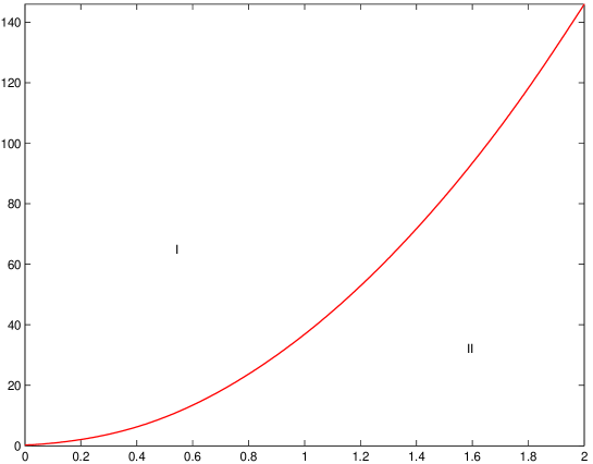
Figure 1: $m$ versus $\alpha_{2}$ for $q=0$, $d=7$, and $\alpha_{3}=3\alpha_{2}/2$.

Unlike to the case of solutions with special values of $\alpha_{2}$ and $\alpha_{3}$ given in Sec. III, the uncharged solution for arbitrary values of fundamental constants $\alpha_{2}$ and $\alpha_{3}$ can have horizon even for $d>9$. Figure 2 shows the function $f(r)$ for $d=10$ as a function of $r$. It shows that there is an event horizon at $r=2$.

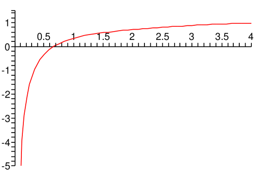
Figure 2: $f(r)$ versus $r$ for $d=10$, $q=0$, $m=500$, $\alpha_{2}=1.0$, and $\alpha_{3}=2.0$.

To investigate the first law of thermodynamics for the solutions with arbitrary values of $\alpha_{2}$ and $\alpha_{3}$, one should perform a numerical analysis. Using the expression for the entropy and the charge given in Eqs. (23) and (24), and the fact that $M=[\Sigma_{d-2}/(16\pi)]m$, where $m$ is the solution of $f(m,r_{+})=0$, one can show numerically that the temperature and electric potential of Eq. (28) are exactly equal to the temperature and electric potential which can be computed through the use of geometrical analysis. Thus, the first law of thermodynamics is valid for the general solution given in Eq. (32). Also, one can perform a stability analysis in canonical and grand-canonical ensembles numerically. Again, as in the case of special solutions of third order Lovelock gravity, numerical analysis shows that there exist only an intermediate stable phase for black hole solutions which is smaller in grand-canonical ensemble .

VI CLOSING REMARKS

In this paper, we added the third order Lovelock terms to the Gauss-Bonnet-Maxwell action, and introduced a new class of static solutions which are asymptotically flat, AdS or dS for $\Lambda=0$, $\Lambda<0$ or $\Lambda>0$ respectively. We were only interested in the asymptotically flat solutions.

First, we consider the solutions for special values of $\alpha_{2}$ and $\alpha_{3}$ given in Eq. (14). For uncharged solutions, we found that for $\alpha>0$, the solutions present black holes provided the mass is larger than a critical value, $m_{\mathrm{crit}}$, given in Eq. (16). For negative $\alpha$, they present black holes with two inner and outer horizons for $m>m_{\mathrm{ext}}$, extreme black holes for $m=m_{\mathrm{ext}}$ or naked singularity for $m<m_{\mathrm{ext}}$, where $m_{\mathrm{ext}}$ is given in Eq. (18). These kind of uncharged solutions exist only in third order Lovelock gravity and do not happen in Einstein or Gauss-Bonnet gravity. For the case of charged solutions, we found that there exists an extremal value of $r_{+}$, given by Eq. (19), that determines whether the solution presents a black holes with two inner and outer horizons, an extreme black hole or a naked singularity. Accordingly we obtained temperature, entropy, charge , electric potential and mass of these black hole solutions. We also investigated the first law of thermodynamics, and found that these thermodynamics quantities satisfy the first law of thermodynamics. Also, we performed a stability analysis in canonical ensemble by considering the heat capacity of the solution and found that there exist two unstable phases separated by an intermediate stable phase. This analysis was also done through the use of the determinant of the Hessian matrix of $M(S,Q)$ with respect to its extensive variables and we got the same phase behavior with a smaller region of stability in the grand-canonical ensemble or no stable phase depending on the values of black hole’s parameters.

Second, we introduced the general solution of third order Lovelock gravity for arbitrary values of $\alpha_{2}$ and $\alpha_{3}$ and investigate its properties. Numerical analysis showed that these solutions may be interpreted as black hole solutions with two inner and outer event horizons, extreme black holes or naked singularity depending on the parameters of the solutions. We also found that the conserved and thermodynamics quantities for these general solutions satisfy first law of thermodynamics. Again, the stability analysis showed that there exists only an intermediate stable phase, for the black hole solutions which is smaller for the grand-canonical ensemble.

As we mention, the asymptotically flat solutions obtained in Chr contain only one fundamental constant. Finding new solutions in continued Lovelock gravity with more fundamental constants remains to be carried out in future. Also, the generalization of these solutions to the case of rotating solutions will be given elsewhere.

References

- (1) M. B. Greens, J. H. Schwarz and E. Witten, Superstring Theory, (Cambridge University Press, Cambridge, England, 1987); D. Lust and S. Theusen, Lectures on String Theory, (Springer, Berlin, 1989); J. Polchinski, String Theory, (Cambridge University Press, Cambridge, England, 1998).
- (2) B. Zwiebach, Phys. Lett. B156, 315 (1985); B. Zumino, Phys. Rep. 137, 109 (1986).
- (3) D. Lovelock, J. Math. Phys. 12, 498 (1971); N. Deruelle and L. Farina-Busto, Phys. Rev. D 41, 3696 (1990); G. A. MenaMarugan, ibid. 46, 4320 (1992); 4340 (1992).
- (4) D. G. Boulware and S. Deser, Phys. Rev. Lett., 55, 2656 (1985); J. T. Wheeler, Nucl. Phys. B268, 737 (1986).
- (5) J. T. Wheeler, Nucl. Phys. B273, 732 (1986).
- (6) D. L. Wiltshire, Phys. Lett. B 169, 36 (1986).
- (7) D. L. Wiltshire, Phys. Rev. D 38, 2445 (1988).
- (8) R. G. Cai and K. S. Soh, Phys. Rev. D 59, 044013 (1999); R. G. Cai, ibid. 65, 084014 (2002).
- (9) Y. M. Cho and I. P. Neupane, Phys. Rev. D 66, 024044 (2002).
- (10) R. C. Myers and J. S. Simon, Phys. Rev. D 38, 2434 (1988); R. C. Myers, Nucl. Phys. B289, 701 (1987).
- (11) J. E. Lidsey, S. Nojiri and S. D. Odintsov, J. High Energy Phys., 06, 026 (2002); M. Cvetic, S. Nojiri, S. D. Odintsov, Nucl. Phys. B628, 295 (2002); S. Nojiri and S. D. Odintsov, Phys. Lett. B 521, 87 (2001); ibid. 523, 165 (2001).
- (12) M. H. Dehghani, Phys. Rev. D 67, 064017 (2003); ibid. 69, 064024 (2004); ibid. 70, 064019 (2004).
- (13) M. Banados, C. Teitelboim and J. Zanelli, Phys. Rev. D 49, 975 (1994).
- (14) R. Aros, R. Troncoso and J. Zanelli, Phys. Rev. D 63, 084015 (2001).
- (15) J. P. Muniain and D. Piriz, Phys. Rev. D 53, 816 (1996).
- (16) J. Crisostomo, R. Troncoso and J. Zanelli, Phys. Rev. D 62, 084013 (2000).
- (17) T. Clunan, S. F. Ross and D. J. Smith, Class. Quant. Grav. 21, 3447 (2004).
- (18) F. Muller-Hoissen, Phys. Lett. B 163, 106 (1985).
- (19) J. D. Beckenstein, Phys. Rev. D 7, 2333 (1973); S. W. Hawking, Nature (London) 248, 30 (1974); G. W. Gibbons and S. W. Hawking, Phys. Rev. D 15, 2738 (1977).
- (20) C. J. Hunter, Phys. Rev. D 59, 024009 (1999); S. W. Hawking, C. J. Hunter and D. N. Page, ibid. 59, 044033 (1999); R. B. Mann, ibid. 60, 104047 (1999); ibid. 61, 084013 (2000);
- (21) M. Lu and M. B. Wise, Phys. Rev. D 47, R3095,(1993); M. Visser, ibid. 48, 583 (1993).
- (22) T. Jacobson and R. C. Myers, Phys. Rev. Lett. 70, 3684 (1993); R. M. Wald, Phys. Rev. D 48, R3427, (1993); M. Visser, ibid. 48, 5697 (1993); T. Jacobson, G. Kang and R. C. Myers, ibid. 49, 6587,(1994); V. Iyer and R. M. Wald, ibid. 50, 846 (1994).
- (23) M. M. Caldarelli, G. Cognola and D. Klemm, Class. Quantum Grav. 17, 399 (2000).
- (24) M. Cvetic and S. S. Gubser, J. High Energy Phys. 04, 024 (1999).
- (25) S. S. Gubser and I. Mitra, J. High Energy Phys., 08, 018 (2001).