RESCEU-11/05

RIKEN-TH-47

hep-th/0506221

June 2005

We investigate the general solution with the symmetry $ISO(1,p)\times SO(9-p)$ of Type II supergravity (the three-parameter solution) from the viewpoint of the superstring theory. We find that one of the three parameters ($c_{1}$) is closely related to the “dilaton charge” and the appearance of the dilaton charge is a consequence of deformations of the boundary condition from that of the boundary state for BPS D-branes. We give three examples of the deformed D-branes by considering the tachyon condensation from systems of D$p$D̄$p$-branes, unstable D9-branes and unstable D-instantons to the BPS saturated D$p$-branes, respectively. We argue that the deformed systems are generally regarded as tachyonic and/or massive excitations of the open strings on D$p$D̄$p$-brane systems.

1 Introduction and Overview

Black holes are important objects to investigate the nature of space-time beyond the description by the general relativity. For example, the study of the black hole entropy provides the holographic principle [1], which gives a strong constraint to the property of quantum gravity. The microscopic properties of black holes are also intensively investigated from the viewpoint of string theory. For example, many black hole (or brane) solutions are known in the low energy effective theory of the superstring theory. In particular, for BPS saturated solutions of Type II (or Type I) supergravity, it is well known that there is a correspondence between the classical solutions and the systems of the BPS D-branes [2]. In this sense, it is natural to assume that there is a stringy origin for a general classical solution of Type II supergravity, even for non-BPS systems.

In our previous paper [3], we treated a general classical solution of Type II supergravity with the symmetry $ISO(1,p)\times SO(9-p)$, which is called as the “three-parameter solution” [4]. The solution had been thought to be the low energy counterpart of the D$p$D̄$p$-brane system with a constant tachyon profile (vacuum expectation value (VEV)), where the three parameters had been supposed to correspond to the number of the D-branes, that of the anti D-branes and the VEV of the tachyon field [5, 6]. In [3], however, we re-examined this correspondence and found that the above conjecture is not correct and the three-parameter solution is the low energy counterpart of the D$p$D̄$p$-brane system with a constant tachyon VEV only if one of the three parameters, $c_{1}$, is tuned to zero.

In this paper, we consider the stringy interpretation of missing $c_{1}$ and give some explicit examples of the stringy counterparts of the three-parameter solution. As we mentioned in the previous paper [3], $c_{1}$ is related to the “dilaton charge”, which characterizes the asymptotic behavior of the dilaton field. It is well known that black holes with horizons do not have the dilaton charge in general, which is supported by the no-hair theorem, but some exceptions are known [2, 7, 8] and we have not understood this phenomena systematically [9]. One of the purposes of this paper is to give an approach to this problem from the microscopic (string theoretical) point of view.

Our strategy is making use of the known correspondence between the BPS black $p$-brane solution in the supergravity and the BPS D$p$-branes in the string theory, and extending this correspondence by appropriately deforming the both sides. On the supergravity side, this leads to a new characterization of the solution. We will find that the BPS limit of the three-parameter solution consists of two extremal limit, that is, the ordinary BPS condition and the condition that the dilaton charge is proportional to the ADM mass. Then, the three-parameter solution is characterized by two non-extremality parameters (and the RR-charge). In particular, the parameter $c_{1}$ is related to the second non-extremality. On the string theory side, we will formally deform the boundary state for the BPS D$p$-brane, which respects the same symmetry of the three-parameter solution. By evaluating the long distance behavior of the solution of the supergravity and the massless emission from the deformed boundary state, we will directly compare the (microscopic) deformation parameters of the boundary state and the (macroscopic) parameters in the three-parameter solution. From this analysis, we show that the first kind of non-extremality corresponds to the non-BPS nature, while the second kind (hence $c_{1}$) is related to the deformation of the boundary condition from the ordinary Neumann/Dirichlet one.

As examples of the deformed boundary states, we consider three systems of D-branes. The first one is the system we consider in [3], which possesses only the first non-extremality since the D$p$D̄$p$-system follows the ordinary boundary condition, that is, the Neumann boundary condition for the longitudinal directions and the Dirichlet boundary condition for the transverse directions. The second and the third example are systems of unstable D9-branes and unstable D-instantons, respectively, with an appropriate tachyon condensation to the BPS D$p$-branes, which actually have non-trivial dilaton charges, i.e. non-zero value of $c_{1}$. They possess the deformation of the boundary condition for the worldsheet, which represent in some sense fuzziness in transverse or longitudinal directions, respectively. From these examples, we discuss that deformed boundary states which respect the symmetry of the three-parameter solution can be obtained by considering D$p$D̄$p$-systems on which tachyonic and/or massive excitations are turned, in general.

The organization of this paper is as follows. In the next section, we review the three-parameter solution and we propose a new characterization of the solution in terms of two non-extremality parameters. In the section 3, we give the string theoretical interpretation to the parameter $c_{1}$ and give three examples of the deformed boundary states. The section 4 is devoted to the conclusions and discussions.

2 The Three-Parameter Solution and Non-Extremalities

In this section, we first give a short review of the three-parameter solution. Then, by investigating the BPS limit of the solution, we propose a new characterization of the solution in terms of two non-extremality parameters.

First of all, we consider Type II supergravity in the following setting:

• Assume a fixed, $(p+1)$-dimensional object as a source carrying only RR $(p+1)$-form charge.

• Spacetime has the symmetry $ISO(1,p)\times SO(9-p)$ and it is asymptotically flat.

Note that these ansatzes are the same as those for the BPS black $p$-brane solution (we will consider the region $0\leq p\leq 6$ in this paper). Under these conditions, it is sufficient to consider the metric, the dilaton and the RR $(p+1)$-form field. The relevant part of the ten-dimensional action (in the Einstein frame) is given by

$$S=\frac{1}{2\kappa^{2}}\int d^{10}x\sqrt{-g}\left[R-\frac{1}{2}(\partial\phi)^{2}-\frac{1}{2(p+2)!}e^{\frac{3-p}{2}\phi}|F_{p+2}|^{2}\right],$$ (2.1)

where $F_{(p+2)}$ denotes the $(p+2)$-form field strength which is related to the $(p+1)$-form potential of the RR-field $\mathcal{A}^{(p+1)}$ as $F_{(p+2)}=d\mathcal{A}_{(p+1)}$. According to the symmetry $ISO(1,p)\times SO(9-p)$, we should impose the following ansatz,

$$ds^{2} =g_{MN}dx^{M}dx^{N}$$

$$=e^{2A(r)}\eta_{\mu\nu}dx^{\mu}dx^{\nu}+e^{2B(r)}\delta_{ij}dx^{i}dx^{j}$$

$$=e^{2A(r)}\eta_{\mu\nu}dx^{\mu}dx^{\nu}+e^{2B(r)}(dr^{2}+r^{2}d\Omega_{(8-p)}^{2}),$$

$$\phi =\phi(r),$$

$$\mathcal{A}^{(p+1)} =e^{\Lambda(r)}\ dx^{0}\wedge dx^{1}\wedge\cdots\wedge dx^{p},$$ (2.2)

where $M=(\mu,i)$, $\mu,\nu=0,\cdots,p$ are indices of the longitudinal directions of the $p$-brane, $i,j=p+1,\cdots,9$ express the orthogonal directions, and $r^{2}=x^{i}x_{i}$.

The authors of [4] gave a general solution of Type II supergravity of this system. As the solution includes three integration constants, it is called as the three-parameter solution, which is given by

$$A(r) =\frac{(7-p)(3-p)c_{1}}{64}h(r)-\frac{7-p}{16}\ln\left[\cosh(kh(r))-c_{2}\sinh(kh(r))\right],$$ (2.3)

$$B(r) =\frac{1}{7-p}\ln[f_{-}(r)f_{+}(r)]$$

$$\hskip 14.22636pt-\frac{(p+1)(3-p)c_{1}}{64}h(r)+\frac{p+1}{16}\ln\left[\cosh(kh(r))-c_{2}\sinh(kh(r))\right],$$ (2.4)

$$\phi(r) =\frac{(p+1)(7-p)c_{1}}{16}h(r)+\frac{3-p}{4}\ln\left[\cosh(kh(r))-c_{2}\sinh(kh(r))\right],$$ (2.5)

$$e^{\Lambda(r)} =-\eta(c_{2}^{2}-1)^{1/2}\ \frac{\sinh(kh(r))}{\cosh(kh(r))-c_{2}\sinh(kh(r))},$$ (2.6)

where

$$f_{\pm}(r) \equiv 1\pm\frac{r_{0}^{7-p}}{r^{7-p}},$$ (2.7)

$$h(r) \equiv\ln\left(\frac{f_{-}}{f_{+}}\right),$$ (2.8)

$$k \equiv\pm\sqrt{\frac{2(8-p)}{7-p}-\frac{(p+1)(7-p)}{16}c_{1}^{2}}$$

$$\equiv\pm\frac{\sqrt{(p+1)(7-p)}}{4}\,\sqrt{c_{m}^{2}-c_{1}^{2}},\qquad\left(c_{m}=\sqrt{\frac{32(8-p)}{(p+1)(7-p)^{2}}}\right),$$ (2.9)

$$\eta \equiv\pm 1,$$ (2.10)

where $\eta$ denotes the sign of the RR-charge. The three parameters, $r_{0},\ c_{1},\ c_{2}$, are the integration constants that parametrize the solution. As in [5], the domain of the parameters in the solution (2.3)–(2.6) we take is

$$c_{1} \in[0,c_{m}],$$ (2.11)

$$c_{2} \in(-\infty,-1]\cup[1,\infty),$$ (2.12)

$$r_{0}^{7-p} \in{\mathbf{R}}.$$ (2.13)

where we have already fixed the ${\mathbf{Z}}_{2}$ symmetries of the solution,

$$(r_{0}^{7-p},c_{1},c_{2},sgn(k),\eta) \to(r_{0}^{7-p},c_{1},-c_{2},-sgn(k),-\eta),$$

$$(r_{0}^{7-p},c_{1},c_{2},sgn(k),\eta) \to(-r_{0}^{7-p},-c_{1},c_{2},-sgn(k),\eta),$$ (2.14)

by choosing $c_{1}\geq 0$ and $k\geq 0$. Furthermore, we have a degree of freedom to choose the signs of $r_{0}^{7-p}$ and $c_{2}$. As we mentioned in Sec.1, we will discuss the BPS black $p$-brane limit of the three-parameter solution and in order to take that limit consistently, we must choose one of the two branches,

$$\begin{cases}r_{0}^{7-p}\geq 0,\ c_{2}>0&\mbox{: branch}\ I_{+},\\ r_{0}^{7-p}\leq 0,\ c_{2}<0&\mbox{: branch}\ I_{-}.\end{cases}$$ (2.15)

From the viewpoint of the gravity theory, the three-parameter solution describes charged dilatonic black objects. Thus, the RR-charge $Q$, the ADM mass $M$ and the dilaton charge $D$ are natural quantities to characterize the solution. For convenience, we consider wrapping the spatial worldvolume directions on a torus $T^{p}$ of volume $V_{p}$. The RR-charge is given by an appropriate surface integral over the sphere-at-infinity in the transverse directions [5, 10];

$$|Q|=2(c_{2}^{2}-1)^{1/2}kN_{p}r_{0}^{7-p},$$ (2.16)

where

$$N_{p}\equiv\frac{(8-p)(7-p)\omega_{8-p}V_{p}}{16\kappa^{2}},$$ (2.17)

and $\omega_{d}=\frac{2\pi^{(d+1)/2}}{\Gamma((d+1)/2)}$ is the volume of the unit sphere $S^{d}$. The ADM mass is defined in [11, 12] as

$$g_{00}=-1+\frac{7-p}{8}\frac{M}{N_{p}}\frac{1}{r^{7-p}}+\mathcal{O}\left(\frac{1}{r^{2(7-p)}}\right),$$ (2.18)

where (2.17) is used. This gives us [5]

$$M=\left(2c_{2}k+\frac{3-p}{2}c_{1}\right)N_{p}r_{0}^{7-p},$$ (2.19)

Similarly, we define the dilaton charge by its asymptotic behavior in the transverse direction as [13]

$$\phi=\frac{D}{N_{p}}\frac{1}{r^{7-p}}+\mathcal{O}\left(\frac{1}{r^{2(7-p)}}\right),$$ (2.20)

which gives

$$D=\left(\frac{3-p}{2}c_{2}k-\frac{(p+1)(7-p)}{8}c_{1}\right)N_{p}r_{0}^{7-p}.$$ (2.21)

Here we give some historical remarks on the dilaton charge. As we referred in [3], the dilaton charge is a familiar quantity in the general relativity [14, 15, 16, 17] and it has been investigated for a long time in various contexts, for example, the no-hair theorem [18], the cosmic censorship, the scalar field collapse [19]. It is well known that the existence of the dilaton charge would change the structures of spacetimes drastically [16, 9, 20] and generally cause naked singularities to appear. The extensions to the higher-dimensional theories [21] or the stabilities of such singular spacetimes have been also investigated by many authors [22, 23]. In spite of those investigations, we have not systematically understood the relation between the horizon and the dilaton charge, for example, what kind of the dilaton couplings to the RR-charge can avoid to make a spacetime singular.

Since the three-parameter solution is the most general solution with the symmetry $ISO(1,p)\times SO(9-p)$, it naturally includes the BPS black $p$-brane solution;

$$ds^{2} = f(r)^{-\frac{7-p}{8}}\eta_{\mu\nu}dx^{\mu}dx^{\nu}+f(r)^{\frac{p+1}{8}}\delta_{ij}dx^{i}dx^{j},$$ (2.22)

$$e^{\phi}(r) = f(r)^{\frac{3-p}{4}},$$ (2.23)

$$e^{\Lambda(r)} = -\eta\left(f(r)^{-1}-1\right),$$ (2.24)

where

$$f(r)=1+\frac{\mu_{0}}{r^{7-p}}.$$ (2.25)

Note that $\mu_{0}$ is the only parameter of the solution, and therefore, all the quantities are labeled by it as

$$|Q|=M=N_{p}\mu_{0},\qquad D=\frac{3-p}{4}N_{p}\mu_{0},$$ (2.26)

where $\mu_{0}$ takes an arbitrary non-negative value. In this paper, we will restrict ourselves to the charged case, i.e., $\mu_{0}>0$.

As we claimed in [3], the parametrization by $(c_{1},c_{2},r_{0})$ is not suitable to take the BPS limit, and so we defined a set of parameters $(c_{1},\mu_{0},\nu)$ which was defined by

$$r_{0}^{7-p}\equiv\frac{\nu\mu_{0}}{2k},\qquad c_{2}^{2}-1\equiv\frac{1}{\nu^{2}}.$$ (2.27)

The domain of $\nu$ becomes

$$\begin{cases}0\leq\nu<\infty&\mbox{for the branch}\ I_{+},\\ -\infty<\nu\leq 0&\mbox{for the branch}\ I_{-},\end{cases}$$ (2.28)

since we choose $c_{1}\geq 0,\ k\geq 0$ and $\mu_{0}>0$. Using these parameters, the RR-charge, the ADM mass and the dilaton charge are rewritten as

$$|Q| =N_{p}\mu_{0},$$ (2.29)

$$M =\left(\sqrt{1+{\nu^{2}}}+\frac{3-p}{4}\frac{c_{1}\nu}{k}\right)N_{p}\mu_{0},$$ (2.30)

$$D =\left(\frac{3-p}{4}\sqrt{1+{\nu^{2}}}-\frac{(p+1)(7-p)}{4}\frac{c_{1}\nu}{k}\right)N_{p}\mu_{0}=\frac{3-p}{4}M-\frac{c_{1}\nu}{k}N_{p}\mu_{0}.$$ (2.31)

Then, it is easy to show that the three-parameter solution (2.3)–(2.6) reduces to the BPS black $p$-brane solution (2.22)–(2.24) in the limit $\nu\rightarrow 0$ for arbitrary values of $c_{1}$ and $\mu_{0}$. Since $|Q|$ is unchanged in this limit, we can set $\mu_{0}$ to the same value as the black $p$-brane. We emphasize here that since there are three parameters, the BPS limit consists of two extremal limits, i.e. $M=|Q|$ and $D=\frac{3-p}{4}M$. The former is the ordinary BPS condition, which guarantees the preservation of the spacetime supersymmetry. Although the latter says that the dilaton charge is proportional to the ADM mass, its physical meaning is obscure at this stage. Nevertheless, if we take the BPS limit as a starting point, it is quite natural to characterize the solution by two non-extremality parameters, that represent the deviation from the BPS black $p$-brane solution.

From this observation, we introduce following quantities $m$ and $d$ defined by

$$m =\sqrt{1+\nu^{2}},$$ (2.32)

$$d =\frac{c_{1}\nu}{k},$$ (2.33)

which are related to the quantities above as

$$|Q| =N_{p}\mu_{0},$$ (2.34)

$$M =\left(m+\frac{3-p}{4}d\right)N_{p}\mu_{0},$$ (2.35)

$$D =\left(\frac{3-p}{4}m-\frac{(p+1)(7-p)}{16}d\right)N_{p}\mu_{0}.$$ (2.36)

The region of these quantities are determined as

$$\begin{cases}m\geq 1,\ d\geq 0&\mbox{for the branch}\ I_{+},\\ m\geq 1,\ d\leq 0&\mbox{for the branch}\ I_{-}.\end{cases}$$ (2.37)

The BPS solution lies in $m=1$ and $d=0$ in the overlap of $I_{+}$ and $I_{-}$. Note that the ADM mass and the dilaton charge are not conserved Noether charges and are frame-dependent quantities. Although their definition is ambiguous in some sense, they can characterize the deviation from the Minkowski space. On the other hand, our quantities $m$ and $d$ represent the deviation from the BPS black $p$-brane solution. As opposed to the ADM mass $M$, $m$ is always greater than $1$. Hence, $m$ can be considered as a non-extremality parameter in the ordinary sense, while $d$ denotes the difference between the ADM mass $M$ and the dilaton charge $D$. Note that $d$ is related to the parameter $c_{1}$ directly. As we have shown in [3], the three-parameter solution with $c_{1}=0$ denotes the spacetime which is produced from the D$p$D̄$p$-brane system with a constant tachyon VEV. Since a main purpose of this paper is to clarify the stringy meaning of $c_{1}$, our task is to find sources in the string theory which produces $d\neq 0$ structure.

At the end of this section, we give the long distance behavior of the three-parameter solution (2.3)–(2.6), which is given by the leading term of $1/r$ expansion. In terms of $(\mu_{0},m,d)$ it is given by

$$e^{2A(r)} =1-\frac{7-p}{8}\left(m+\frac{3-p}{4}d\right)\frac{\mu_{0}}{r^{7-p}}+{\cal O}\left(1/r^{2(7-p)}\right),$$ (2.38)

$$e^{2B(r)} =1+\frac{p+1}{8}\left(m+\frac{3-p}{4}d\right)\frac{\mu_{0}}{r^{7-p}}+{\cal O}\left(1/r^{2(7-p)}\right),$$ (2.39)

$$\phi(r) =\left(\frac{3-p}{4}m-\frac{(p+1)(7-p)}{16}d\right)\frac{\mu_{0}}{r^{7-p}}+{\cal O}\left(1/r^{2(7-p)}\right),$$ (2.40)

$$e^{\Lambda(r)} =\eta\frac{\mu_{0}}{r^{7-p}}+{\cal O}\left(1/r^{2(7-p)}\right).$$ (2.41)

We will compare them with the massless emission from the source in the string theory in the next section.

3 Excitations on the D$p$D̄$p$-brane System

In this section, we investigate stringy counterparts of the three-parameter solution. We argue that the geometry expressed by the three-parameter solution is made by D-brane systems which are in general sources of closed strings in the bulk. We stress that we only consider static sources and do not take into account interactions of open strings on the D-brane. Therefore they can be consistent sources of supergravity fields, even if they are unstable system. As a first step, we deform the boundary state for BPS D$p$-branes appropriately, and compare the long distance behavior of the solution with the massless emissions from them. And then, we give some examples.

3.1 Deformations of Boundary States

To obtain the three-parameter solution, we have required that the solution has the symmetry $ISO(1,p)\times SO(9-p)$ and it carries a RR $(p+1)$-form charge as explained in the previous section. Therefore the source of closed strings, which produces the three-parameter solution, should respect the following restrictions at least in the low energy regime;

$$1)\quad \text{has the symmetry $ISO(1,p)\times SO(9-p)$},$$

$$2)\quad (p+1)$$ carries only the RR -form charge, (3.1)

$$3)\quad \delta$$ has the -function distribution in the transverse space.

Note that the third condition can be slightly relaxed (see below).

Needless to say, the system of coincident BPS D$p$-branes is such an example. $N$ BPS D$p$-branes are expressed by the boundary state,

$$\left|\,{Dp}\,\right\rangle={\cal P}_{\rm GSO}\Bigl{(}N\left|\,{Bp}\,\right\rangle_{\rm NS}+N\left|\,{Bp}\,\right\rangle_{\rm RR}\Bigr{)},$$ (3.2)

with

$$\left|\,{Bp}\,\right\rangle_{\rm NS(RR)}=\frac{T_{p}}{2}\exp\left[{-\sum_{n=1}^{\infty}\frac{1}{n}\alpha_{-n}^{M}S_{MN}\widetilde{\alpha}_{-n}^{N}}+i\sum_{r>0}^{\infty}b_{-r}^{M}S_{MN}\widetilde{b}_{-r}^{N}\right]\left|\,{p_{\mu}=0,x^{i}=0}\,\right\rangle_{\rm NS(RR)},$$ (3.3)

where $T_{p}$ is the tension for a single D$p$-brane, $\mu=0,1,\cdots,p$ are the directions longitudinal to the worldvolume, $i=p+1,\cdots,9$ are the directions transverse to the D$p$-branes, and $\alpha_{-n}^{M}$ and $b_{-r}^{M}$ ($\widetilde{\alpha}_{-n}^{M}$ and $\widetilde{b}_{-r}^{M}$) are the creation operators of the modes of the left-moving (right-moving) worldsheet bosons and fermions, respectively. $S_{MN}={\rm diag}\left(\eta_{\mu\nu},-\delta_{ij}\right)$ gives Neumann (Dirichlet) boundary conditions on the string worldsheet in $\mu(i)$ directions, respectively. Here the number of the D$p$-branes $N$ is the only microscopic parameter. In this case, it is shown that massless emission from this boundary state agrees with the long distance behavior of the BPS black $p$-brane [24] under the identification,

$$\mu_{0}=\frac{2\kappa NT_{p}}{(7-p)\omega_{8-p}},$$ (3.4)

which relates the macroscopic parameter $\mu_{0}$ with the microscopic parameter $N$. Of course, the system with $\bar{N}$ $\bar{\rm D}p$-brane also satisfies the same ansatz, which is simply given by replacing $N$ to $-\bar{N}$ in the RR-sector of (3.2). We can also consider the system with $N$ D$p$-branes and $\bar{N}$ D̄$p$-branes without tachyon field which is given by the linear combination of the both above.

We now take the BPS boundary state (3.2) as the starting point as mentioned in Sec.1 and consider possible deformations of it with keeping the ansatzes (3.1), which should be the counterpart of the discussion in Sec.2, that is, on the supergravity side. One might try to deform it with massless open string excitations on the brane. However, the symmetry $ISO(1,p)\times SO(9-p)$ prevents the fluctuation of massless scalar fields, and there should be no gauge flux since otherwise it produces other NSNS/RR-charges. Therefore, the excitations on the branes should be at least tachyonic and/or massive.

In order to make the discussion transparent, we formally deform the boundary state as follows. In the NSNS-sector, we set

$$\left|\,{B_{p}^{\prime}}\,\right\rangle_{NS}=CN\frac{T_{p}}{2}\exp\left[-\sum_{n=1}^{\infty}\frac{1}{n}\alpha_{-n}^{M}S_{MN}^{(n)}\widetilde{\alpha}_{-n}^{N}+i\sum_{r>0}b_{-r}^{M}S_{MN}^{(r)}b_{-r}^{N}\right]\left|\,{p_{\mu}=0,x^{i}=0}\,\right\rangle_{NS},$$ (3.5)

where

$$S_{MN}^{(n,r)}={\rm diag}\left(A^{(n,r)}\eta_{\mu\nu},-B^{(n,r)}\delta_{ij}\right).$$ (3.6)

Here $A^{(n,r)}$, $B^{(n,r)}$ and $C$ are deformation parameters which deform the boundary state without changing its symmetry. When we take $A^{(n,r)}=B^{(n,r)}=C=1$, the boundary state (3.3) for the $N$ BPS D$p$-branes is reproduced. We also deform the RR-sector of the boundary state (3.3) as the same manner but $C=1$ in this case since we fix the RR-charge to be the same as the $N$ D$p$-branes. We give some comments in order. First, one might assume the source object is a $\delta$-function type located at the origin in the transverse space. But it will turn out to be too restrictive and can be relaxed slightly: the “width” of the source allowed to be less than the string length. We will come back to this point in the next subsection. Second, the effect of $(A^{(n,r)},B^{(n,r)})$ in $S_{MN}^{(n,r)}$ is the deformation of the boundary condition. Here we note that only the $r=1/2$ mode contributes the massless mode of closed strings emitted from the boundary state. In other words, the deformations for other modes, $S_{MN}^{(n)}$ and $S_{MN}^{(r\neq 1/2)}$, are arbitrary in our analysis below. However, they should be related among them by other consistency, such as the modular invariance although we do not discuss them at this stage. Third, $C$ denotes the difference of the overall normalization in the NSNS-sector from that in the RR-sector. For example, in the system of $(N+M)$ D$p$-branes and $M$ $\bar{\rm D}p$-branes, we take $CN=N+2M$, the total number of branes, while the RR-sector has a fixed charge proportional to $N$.

Then, we can calculate the massless emissions with momentum $p_{M}$ from this deformed state as we have done in [3]. In the NSNS-sector there are the graviton $h_{MN}$ and the dilaton $\phi$, that are

$$f(p) = \left\langle\,{f(p)}\,\right|\Delta\left|\,{D^{\prime}p}\,\right\rangle=-CN\frac{T_{p}}{2}\frac{V_{p+1}}{p_{i}^{2}}\epsilon_{MN}^{f}S^{(1/2)MN},$$ (3.7)

where $\left|\,{D^{\prime}p}\,\right\rangle$ denotes the GSO projected deformed state, $\Delta$ is the closed string propagator and $\epsilon_{MN}^{f}$ is the appropriate polarization tensor for $f=h_{MN},\phi$ [3]. There is a similar expression for the RR $(p+1)$-form $e^{\Lambda}$. In this case, since we set $C=1$ for the RR-sector and since only the zero-mode part contributes to the massless fields, we obtain same result as the BPS D$p$-brane. After the Fourier transformation to the position space, we obtain

$$h_{MN}(r) =\left(-\frac{7-p}{8}\eta_{\mu\nu},\frac{p+1}{8}\delta{ij}\right)\frac{C(A+B)}{2}\frac{2\kappa NT_{p}}{(7-p)\omega_{8-p}}\frac{1}{r^{7-p}},$$ (3.8)

$$\phi(r) =\frac{C}{8}\left[-(p+1)A+(7-p)B\right]\frac{2\kappa NT_{p}}{(7-p)\omega_{8-p}}\frac{1}{r^{7-p}},$$ (3.9)

$$e^{\Lambda}(r) =\pm\frac{2\kappa NT_{p}}{(7-p)\omega_{8-p}}\frac{1}{r^{7-p}},$$ (3.10)

where we write $A=A^{(1/2)}$ and $B=B^{(1/2)}$. Comparing these quantities (3.8)-(3.10) with the long distance behaviors (2.38)-(2.41), we obtain the relation between the macroscopic quantities and the microscopic ones as

$$\mu_{0}=\frac{2\kappa NT_{p}}{(7-p)\omega_{8-p}},$$ (3.11)

$$m=\frac{C}{8}\left[(p+1)A+(7-p)B\right],$$ (3.12)

$$d=\frac{C}{2}(A-B).$$ (3.13)

We see from the eqs. (3.12) and (3.13) that the two non-extremality parameters $m$ and $d$ in the three-parameter solution correspond to the deformation parameter $(A,B,C)$ on the string theory side. The first non-extremality $m\neq 1$ can be realized even if $A=B=1$, by taking $C\neq 1$. It means that the breaking of the BPS condition can occur within the ordinary boundary condition. However, the second non-extremality $d\neq 0$ requires necessarily $A\neq B$. Therefore, in order to have the three-parameter solution with nonzero $c_{1}$, it is necessary to deform the boundary condition from the ordinary one of the BPS D$p$-branes so as to satisfy $A\neq B$. In the next subsection, we give examples of such stringy objects.

3.2 Examples

In this subsection, we give three typical examples realizing the deformed states in the string theory which we referred in the previous subsection by considering various types of the tachyon condensation. The first example is the case considered in [3]. The other two examples are obtained from the tachyon condensation from higher/lower dimensional unstable D-brane systems. In general, deformations are interpreted as tachyonic/massive excitations on the D$p$D̄$p$ system.

3.2.1 Case 1: D$p$D̄$p$ system with a tachyon VEV

The first example is the D$p$D̄$p$ system with a constant tachyon profile. To be precise we consider the $(N+M)$ D$p$-branes and $M$ $\bar{\rm D}p$-branes. The gauge symmetry of the worldvolume theory is $U(N+M)\times U(M)$ and there is a complex tachyon field $T(x)$ in the bi-fundamental representation of the gauge group. Here we consider the case where the $M$ D$p$D̄$p$-pairs vanish and $N$ D$p$-branes remain. Namely, we decompose the $M\times(N+M)$ matrix by $M\times N$ and $M\times M$ components and set the tachyon profile as

$$T(x)=\left(\begin{array}[]{c}0\\ \hline\cr t\end{array}\right),$$ (3.16)

where $t$ is a constant $M\times M$ matrix. Note that other open string excitations, such as gauge fields, massless scalar fields and a non-constant tachyon, break the symmetry $ISO(1,p)\times SO(9-p)$.

It is known that this system can be expressed by the off-shell boundary state on which the boundary interaction for the tachyon field is turned [25, 26]. For our case, the NSNS-sector of the boundary state is then given by

$$\left|\,{B_{p}^{\prime};t}\,\right\rangle_{\rm NS} =\left[N+2{\rm Tr}_{M}\,e^{-|t|^{2}}\right]\frac{T_{p}}{2}\,e^{-\sum_{n=1}^{\infty}\frac{1}{n}\alpha_{-n}^{M}S_{MN}\widetilde{\alpha}_{-n}^{N}+i\sum_{r>0}b_{-r}^{M}S_{MN}\widetilde{b}_{-r}^{N}}\left|\,{p_{\mu}=0,x^{i}=0}\,\right\rangle_{\rm NS},$$ (3.17)

where $S_{MN}=(\eta_{\mu\nu},-\delta_{ij})$ and the trace is taken over $M\times M$ matrices. Note that it is the same as (3.3) except for the overall factor, $\left[N+2{\rm Tr}_{M}\,e^{-|t|^{2}}\right]$, which simply comes from the tachyon potential $V(T)\sim{\rm Tr}e^{-|T|^{2}}$. It reduces to the $N+2M$ in the limit $|t|\rightarrow 0$, corresponding to the $(N+M)$ D$p$-branes and $M$ $\bar{\rm D}p$-branes, while reduces to $N$ in the limit $|t|\rightarrow\infty$, corresponding to the $N$ D$p$-branes.

From this state, we can read off $(A,B,C)$ by comparing (3.17) with (3.5) as

$$A=B=1,\qquad\ C=1+\frac{2}{N}\ {\rm Tr}_{M}\ e^{-|t|^{2}}.$$ (3.18)

Therefore, macroscopic quantities $m$ and $d$ are given by

$$m=1+\frac{2}{N}\ {\rm Tr}_{M}\ e^{-|t|^{2}},\qquad\ d=0.$$ (3.19)

We see that the constant tachyon $t$ only contributes to the ADM mass. Therefore, this system corresponds to at most two-parameter subset of the full three-parameter solution as we mentioned in [3], but it is an trivial example for our present purpose.

3.2.2 Case 2: Unstable D9-branes to BPS D$p$-branes

Next example is the tachyon condensation from unstable D$9$-branes to the BPS D$p$-branes. For simplicity, we consider Type IIB superstring theory, that is, the tachyon condensation from pairs of D9-branes and D̄9-branes to BPS D$p$-branes. For Type IIA superstring theory, we start from non-BPS D9-branes and the discussion is completely parallel. Since a single BPS D$p$-brane is obtained from a pair of D(p+2)-brane and D̄(p+2)-brane, it is clear that it is obtained from $2^{\frac{7-p}{2}}$ pairs of D9-brane and D̄9-brane via the tachyon condensation. Then let us consider $N\times 2^{\frac{7-p}{2}}$ pairs of D9D̄9-branes and the tachyon profile,

$$T(x)=u\gamma_{i}x^{i}\otimes 1_{N},$$ (3.20)

where $i=p+1,\cdots,9$ are the transverse directions to the resulting D$p$-brane, $\gamma_{i}$ are the $SO(9-p)$ gamma matrices and $u$ is a real parameter of dimension of mass. It is known that this system reduces to $N$ BPS D$p$-branes in the limit $u\rightarrow\infty$. If we replace $T$ to $-T$, the final state becomes D̄$p$-branes.

Here the effect of the tachyon profile (3.20) with $u\neq 0$ is twofold: First, it breaks the original global symmetry $ISO(1,9)$ down to $ISO(1,p)\times SO(9-p)$. Next, it produces the correct RR-charge of $N$ D$p$-branes which is independent of the value of $u$. Therefore, this system satisfies the first two items of the ansatzes (3.1) for an arbitrary value of $u\neq 0$. However, accurately speaking, it does not satisfy the third item. In fact, the intermediate state ($0<u<\infty$) is neither D$9$-branes nor D$p$-branes but its energy density in the transverse direction has the Gaussian-shaped distribution with a width $\sim 1/u$. (This is easily seen by noting the tachyon potential has the form $V(T)\sim e^{-u^{2}x^{i}x_{i}}$.) Therefore, if we allow the width of the source less than the string length, $u$ should be sufficiently larger than $1/\sqrt{\alpha^{\prime}}$. We will evaluate it more precisely below.

This system is again described by the off-shell boundary state of the D9D̄9 system with the tachyon profile (3.20) turned on [26]. It is given by in the NSNS-sector,

$$\left|\,{Bp^{\prime};u}\,\right\rangle_{\rm NS}=\frac{T_{9}}{2}\int[d{\mathbf{X}}^{M}]{{\rm Tr}}\widehat{\rm P}e^{\int d\widehat{\sigma}\mathbf{M}(\widehat{\sigma})}\left|\,{{\mathbf{X}}^{M}}\,\right\rangle_{\rm NS},$$ (3.21)

with

$$\mathbf{M}=\left(\begin{array}[]{cc}0&T({\mathbf{X}})\\ T^{\dagger}({\mathbf{X}})&0\end{array}\right),$$ (3.22)

where $T_{9}$ is the tension of a single D$9$-brane, $T(x)$ is given by (3.20) and the trace is taken over the Chan-Paton space of size $2^{\frac{9-p}{2}}N$. It represents the Neumann boundary state with arbitrary numbers of tachyon vertex operators attached. By evaluating the path integral and rewriting it with oscillators, we obtain (see Appendix for more details)

$$\left|\,{Bp^{\prime};u}\,\right\rangle_{\rm NS}= N\frac{T_{p}}{2}\,\ e^{-\frac{1}{4u^{2}}\int\mathbf{P}_{i}D\mathbf{P}_{i}}\left|\,{\mathbf{P}_{\mu}=0,{\mathbf{X}}^{i}=0}\,\right\rangle_{\rm NS}$$ (3.23)

$$= N\frac{T_{p}}{2}F(y)^{9-p}e^{-\sum_{n=1}^{\infty}\frac{1}{n}\alpha_{-n}^{M}S_{MN}^{(n)}\widetilde{\alpha}_{-n}^{N}+i\sum_{r>0}b_{-r}^{M}S_{MN}^{(r)}\widetilde{b}_{-r}^{N}}\int dp_{i}e^{-\frac{p_{i}^{2}}{8\pi u^{2}}}\left|\,{p_{\mu}=0,p_{i}}\,\right\rangle_{\rm NS},$$ (3.24)

where $y\equiv 4\pi\alpha^{\prime}u^{2}$ is a dimensionless parameter, and the function $F(y)$ is given by

$$F(y)\equiv\frac{4^{y}y^{1/2}\Gamma^{2}(y)}{\sqrt{4\pi}\Gamma(2y)},$$ (3.25)

and

$$S_{MN}^{(n)}=\left(\eta_{\mu\nu},-\frac{y-n}{y+n}\delta_{ij}\right),\qquad S_{MN}^{(r)}=\left(\eta_{\mu\nu},-\frac{y-r}{y+r}\delta_{ij}\right).$$ (3.26)

The corresponding state for the RR-sector is similarly obtained.

It is instructive to see the behavior of this state under the change of the value $u$ $(0<u<\infty)$. First of all, we can identify the state (3.24) with the deformed state (3.5) (apart from the zero-mode part) as

$$A^{(n,r)}=1,\qquad B^{(n)}=\frac{y-n}{y+n},\qquad B^{(r)}=\frac{y-r}{y+r},\qquad C=F(y)^{9-p}.$$ (3.27)

$A^{(n,r)}$ is independent of $y$, which means that the tangential directions always satisfy the Neumann boundary condition. On the other hand, $B^{(n,r)}$ is a monotonically increasing function of $y$, starting from $-1$ (Neumann) at $y=0$ and goes to $1$ (Dirichlet) at $y\rightarrow\infty$. It means that the transverse directions satisfy a mixed boundary condition of Dirichlet and Neumann. Roughly speaking, the boundary condition is Dirichlet-like for $B^{(n,r)}<0$ and Neumann-like for $B^{(n,r)}>0$. Probing only by the massless fields, this state has similar feature as the BPS D$p$-branes at least in the range sufficiently larger than $y=1/2$, although other higher modes can be Neumann-like in this region. $C$ behaves as a monotonically decreasing function of $y$ with $C\rightarrow\infty$ for $y\rightarrow 0$ and $C\rightarrow 1$ for $y\rightarrow\infty$. (We give the profile of the function $F(y)$ in Fig.1.)

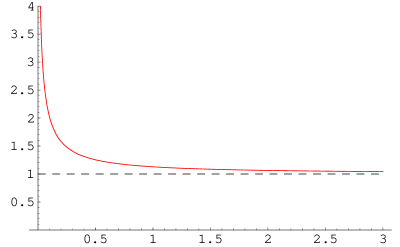
Figure 1: Profile of $F(y)$. The behavior of this function is the same as that of $C$, that is, $C\to\infty$ for $y\to 0$ and $C\to 1$ for $y\to\infty$.

Therefore the effective tension is always greater than that of the BPS D$p$-brane. Although this factor itself is not well-behaved at $y\rightarrow 0$, combined with the contribution from the zero-mode, we recover the correct tension for the D$9$-brane (see Appendix). The zero-mode part depends directly on $u$ and means the Gaussian-shaped distribution in the transverse with a $({\rm width})^{2}=1/{8\pi u^{2}}$. Strictly speaking, this is excluded from our assumption for the deformed state. However, since we only concern the massless emission, it is enough to demand the delta-function source at the low energy, that is, the value of $u$ such that $1/{8\pi u^{2}}\lesssim\alpha^{\prime}$ is in fact well-localized in the limit $\alpha^{\prime}\rightarrow 0$. This condition is equivalent to $y\gtrsim 1/2$, which is the same region discussed previously. When the width is the order of the string scale, then the supergravity approximation is no longer valid and the $\alpha^{\prime}$-correction in the equation of motion and also the source should be taken into account. In this case, the zero-mode factor in (3.24) is nothing but the $\alpha^{\prime}$-corrected $\delta$-function source considered in [29] in the context of the smearing of the singularity.

Thus, at least in the region $y\gtrsim 1/2$, we can identify this microscopic state with the macroscopic quantities as

$$m=F(y)^{9-p}\frac{8y+p-3}{4(2y+1)},\qquad d=F(y)^{9-p}\frac{1}{2y+1}.$$ (3.28)

The behavior of $m$ and that of $d$ as function of $y$ are shown in Fig.2 and Fig.3, respectively.

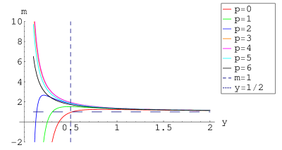
Figure 2: Profiles of $m$’s of the unstable D9-branes for various $p$’s. For the region $y\gtrsim 1/2$, $m$ is very closed to 1, that is, the solution is near extremal in the whole parameter space of the three-parameter solution.

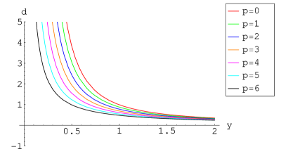
Figure 3: Profiles of $d$’s of the unstable D9-branes for various $p$’s.

Then, we see that they represent a trajectory in the $(m,d)$ space and belong to the branch $I_{+}$: $m\geq 1$, $d\geq 0$. This gives two-parameter subset of the three-parameter solution, which possesses an non-extremal dilaton charge.

As a final remark, we note that the deformation here is also regarded as a massive excitation of open strings on the BPS D$p$-branes, since a tachyonic excitation on the top of the potential is equivalent to the massive excitation from the viewpoint of the bottom (See Fig.4.).

Figure 4: The black circle corresponds to the state in the way of the tachyon condensation from a system of unstable D9-branes to that of BPS D-branes. From the viewpoint of the (false) vacuum (A), it can be regarded as a tachyon excited state. On the other hand, if we look it at from the (true) vacuum (B), it can be regarded as massive excited state.

In fact, the original expression (3.22) represents the deformation of the D9D̄9 system by a tachyonic excitation, while in (3.23) the same system is described by the D$p$-branes with massive vertex operators $\int d\widehat{\sigma}\mathbf{P}_{i}D\mathbf{P}_{i}$ turned on.

3.2.3 Case 3: Unstable D-instantons to BPS D$p$-branes

The third example is the tachyon condensation from a system of unstable D-instantons to the BPS D$p$-branes. In this case, the BPS D$p$-branes can be constructed as bound states of infinitely many unstable D-instantons. For the concreteness, we consider a system of non-BPS D-instantons in Type IIA string theory. There are ten scalar fields $\Phi^{M}$ and a tachyon field $T$ on them. They are regarded as self-adjoint operators acting on the infinite dimensional Hilbert space, since the worldvolume is zero-dimensional and the matrix-size is infinite. Then the configuration representing $N$ BPS D$p$-branes is given by

$$T=v\widehat{p}_{\mu}\otimes\gamma^{\mu}\otimes 1_{N},$$ (3.29)

$$\Phi^{\mu}=\widehat{x}^{\mu}\otimes 1\otimes 1_{N},\qquad\Phi^{i}=0,$$ (3.30)

where $\widehat{x}^{\mu}$ and $\widehat{p}_{\mu}$ are operators on a Hilbert space satisfying the canonical commutation relation,

$$\left[\widehat{x}^{\mu},\widehat{p}_{\nu}\right]=i\delta^{\mu}_{\ \nu},$$ (3.31)

$\mu=0,1,\cdots,p$ are the worldvolume direction and $i=p+1,\cdots,9$ are the transverse direction and $\gamma^{\mu}$ are Hermitian gamma matrices. $v$ is a real parameter with dimension of length and this configuration becomes an exact solution in the limit $v\rightarrow\infty$.

The intermediate state $(0<v<\infty)$ can be interpreted as a $(p+1)$-dimensional object, which has a fuzzy worldvolume in some sense. This is most easily understood as follows. Recall that the each set of eigenvalues of the scalar fields $\{\Phi^{M}\}$ represents the position of each individual D-instanton. In the absence of the tachyon profile $(v=0)$, they are distributed uniformly on the $(p+1)$-dimensional plane, since the spectrum of $\widehat{x}^{\mu}$ spans the real axis. Note that they are still the collection of the D-instantons. However, if we turn on the tachyon profile $(v>0)$, D-instantons become correlated among them. As seen from the tachyon potential $V(T)\sim{\rm Tr}e^{-v^{2}\widehat{p}_{\alpha}\widehat{p}^{\alpha}}$, the momentum distribution is localized around the origin of the momentum space with a width $\Delta p\sim 1/v$. This means (in an appropriate way) that the position of each D-instanton becomes uncertain with an amount of $\Delta x\sim v$. Then, in the limit $v\rightarrow\infty$, it becomes $\Delta x=\infty$ and we cannot observe the individual D-instantons and the worldvolume of D$p$-brane appears.

The off-shell boundary state describing this system is given by the Dirichlet boundary state with the scalar and tachyon fields turned on as the boundary interaction. In the NSNS-sector, after calculating the trace over the Chan-Paton Hilbert space, we have

$$\left|\,{Bp^{\prime};v}\,\right\rangle_{\rm NS}= N\frac{T_{p}}{2}\int\left[d{\mathbf{X}}^{\mu}\right]e^{-\frac{1}{4v^{2}}\int D{\mathbf{X}}^{\mu}D^{2}{\mathbf{X}}^{\mu}}\left|\,{{\mathbf{X}}^{\mu},{\mathbf{X}}^{i}=0}\,\right\rangle_{\rm NS},$$ (3.32)

$$= N\frac{T_{p}}{2}F(y)^{p+1}e^{-\sum_{n=1}^{\infty}\frac{1}{n}\alpha_{-n}^{M}S_{MN}^{(n)}\widetilde{\alpha}_{-n}^{N}+i\sum_{r>0}b_{-r}^{M}S_{MN}^{(r)}\widetilde{b}_{-r}^{N}}\left|\,{p_{\mu}=0,x^{i}=0}\,\right\rangle_{\rm NS},$$ (3.33)

where $y$ is a dimensionless parameter $y\equiv{v^{2}}/{\pi\alpha^{\prime}}$, $F(y)$ is a function,

$$F(y)\equiv\frac{4^{y}y^{1/2}\Gamma^{2}(y)}{\sqrt{4\pi}\Gamma(2y)},$$ (3.34)

and

$$S_{MN}^{(m)}=\left(\frac{y-m}{y+m}\eta_{\mu\nu},-\delta_{ij}\right),\qquad S_{MN}^{(r)}=\left(\frac{y-r}{y+r}\eta_{\mu\nu},-\delta_{ij}\right),$$ (3.35)

which is very similar to (3.24). Then we can identify this state with the deformed state (3.5) with setting the parameters as

$$A^{(n)}=\frac{y-n}{y+n},\qquad A^{(r)}=\frac{y-r}{y+r},\qquad B^{(n,r)}=1,\qquad C=F(y)^{p+1}.$$ (3.36)

Note that the zero-mode part is exactly the delta-function in this case. The boundary condition in the worldvolume direction is now deformed to $A^{(n,r)}$, which connects $A^{(n,r)}=-1$ (Dirichlet) for $y\rightarrow 0$ and $A^{(n,r)}=1$ (Neumann) for $y\rightarrow\infty$. This is understood more easily from the viewpoint of the deformation from the $N$ BPS D$p$-branes, that is, the expression (3.32), on which a massive vertex operator $\frac{1}{4v^{2}}\int D{\mathbf{X}}^{\mu}D^{2}{\mathbf{X}}_{\mu}$ turned . Since such a vertex operator makes the end point of the open string massive, the freely moving endpoint at $y\rightarrow\infty$ becomes heavier and heavier as $y$ decreases, and finally it is completely frozen in the limit of $y\to 0$. The behavior of $C$ as a function of $y$ is the same as the previous example. Here the divergence at $y=0$ is reflected simply by the original system has infinite number of non-BPS D-instantons.

Comparing the massless emission from this state and the long range behavior of the three-parameter solution, we can relate the macroscopic to the microscopic quantities as

$$m=F(y)^{p+1}\frac{8y-p+3}{4(2y+1)},\qquad d=-F(y)^{p+1}\frac{1}{2y+1},$$ (3.37)

and the profiles of these parameters are depicted in Fig.5 and Fig.6.

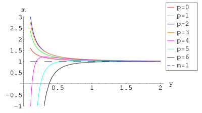
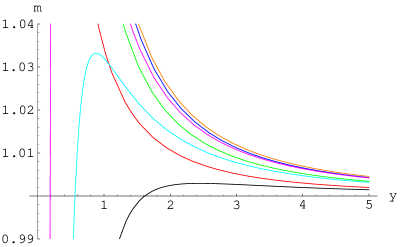
Figure 5: The left figure is the profiles of $m$’s of the system of unstable D-instantons for various $p$’s. The right one is a close-up of the left one around $m=1$. From these figures, it is clear that all $m$’s are always larger than $1$ for sufficiently large $y$ and asymptotically approach $1$ as $y$ increases.

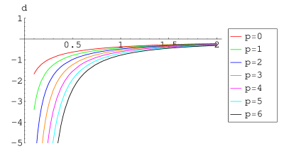
Figure 6: Profiles of $d$’s of the system of unstable D-instantons for various $p$’s. All $d$’s takes arbitrary negative value.

In this case, one might conclude that the description of the supergravity is valid for all region of $y$ since the configuration of D-instantons does not seem to break the ansatzes (3.1). However, as shown in Fig. 5, $m$ is smaller than $1$ if $y$ is too small, which is out of the parameter region of the three-parameter solution. This means that this system is consistent with the three-parameter solution only when $y$ is sufficiently large. This would be understood as follows. As mentioned above, when $v$ $(y)$ is small, the boundary of open strings on the “D-brane” is localized in the tangential directions. From the viewpoint of closed strings, this means that the size of loops that construct the (deformed) boundary state is localized when $y$ is small, that is, the translational invariance is spontaneously broken. This is also related to the uncertainty of the position of D-instantons in the tangential directions. In order to recover the translational invariance of closed string on the brane, the uncertainty must be far larger than the string scale, $\Delta x\sim v\gtrsim\sqrt{\alpha^{\prime}}$, that is, $y\gtrsim 1$ where $m$ is larger than $1$. Since the other non-extremal parameter $d$ is always smaller than 0 (see Fig.6), we conclude that the tachyon condensation from unstable instantons to BPS saturated D$p$-branes is expressed by a three-parameter solution in the branch $I_{-}$: $m\geq 1,d\leq 0$.

3.2.4 Tachyonic/massive excitation on the D$p$D̄$p$ system

We have illustrated three types of deformation above. Here we would like to capture the general feature from above examples and discuss a possible generalization.

First, we summarize the three cases. We considered the situation where the RR-charge is fixed as the same value as $N$ BPS D$p$-branes have. In Case 1, the D$p$D̄$p$ system with an tachyonic excitation gives the three-parameter solution with $d=0$ at low energy, which is trivial in some sense. In Case 2, we considered the tachyon condensation on the D$9$D̄$9$ system, which gives the solutions with $0\leq d$. It is equivalent to the massive excitation on the BPS D$p$-branes. On the other hand, in Case 3, although the tachyon condensation on the unstable D-instanton system is also equivalent to the massive excitation on the BPS D$p$-branes, their low energy solutions have $d\leq 0$. The difference between Case 2 and Case 3 is the polarization of the massive vertex operators: The bosonic part of the vertex operator $\int d\widehat{\sigma}\mathbf{P}_{i}D\mathbf{P}^{i}$ is $\delta_{ij}\int d\sigma\partial_{\tau}X^{i}\partial_{\tau}X^{j}$, which describes the lowest massive mode of open strings, a rank $2$ tensor with zero momentum. On the other hand, the vertex operator $\int d\widehat{\sigma}D{\mathbf{X}}^{\mu}D^{2}{\mathbf{X}}_{\mu}=\eta_{\mu\nu}\int d\sigma\partial_{\sigma}X^{\mu}\partial_{\sigma}X^{\nu}+\cdots$ has a longitudinal polarization. Physically, the effects of transverse (longitudinal) polarization is characterized by the fuzziness of the worldvolume in the transverse (longitudinal) direction, respectively. In the context of the scattering of massive open strings, their difference is argued for example in [35]. We here observe that the difference in the polarization is seen as the sign of $d$ if we probe these systems by massless closed strings.

Next, we discuss the possible generalization of the process of the tachyon condensation. In Case 2 and 3, we have only considered the tachyon condensation to BPS D$p$-branes. However, we can also construct a D$p$D̄$p$ system as long as they have the same RR-charge proportional to $N$, Therefore, recalling that a tachyon excitation on a system of unstable D9-branes or unstable D-instantons is regarded as a massive excitation on the resulting D$p$-branes (see Fig. 4), we can combine the three cases as the D$p$D̄$p$ system with tachyonic and massive excitations. As we have seen above, the tachyonic excitation contributes to $m$ and the massive excitations contribute to both $m$ and $d$. Note that $1\leq m$ in any case.

It is then quite natural to take into account for higher massive excitations. Let us consider vertex operators quadratic in $X$, say,

$$\int d\sigma\partial^{l}_{\tau}X^{i}\partial^{l}_{\tau}X_{i},\quad{\rm or}\quad\int d\sigma\partial^{l}_{\sigma}X^{\mu}\partial^{l}_{\sigma}X_{\mu},$$ (3.38)

with $l=1,2,\cdots$. It is easy to show that such an excitation gives rise to the deformation of the boundary state in the form (3.5). It follows that they also contribute to the three-parameter solution and gives another trajectory in the $(m,d)$ space. Note that the relation between the polarization and the sign of $d$ is unchanged. We can also consider vertex operators with higher power in $X$, unless they break the global symmetry. In this case, the resulting deformed state no longer has the form (3.5) but treating these vertex operators as perturbation, they contribute to the coupling to massless modes of closed strings. In any case, our conclusion is that the D$p$D̄$p$ system with tachyonic and massive excitations are seen as the three-parameter solution at the low energy.

4 Conclusions and Discussions

In this paper, we discussed the stringy origin of the general solution of Type II supergravity with the symmetry $ISO(1,p)\times SO(9-p)$, which is called as the three-parameter solution. This solution contains the BPS saturated black $p$-brane solution in the parameter space, whose source is BPS saturated D$p$-branes expressed by a boundary state. We characterized the three-parameter solution in terms of two non-extremality parameter $m$ and $d$ on the supergravity side. On the other hand, we discussed a class of the deformation of the boundary state on the string side. Then we determined the relation between the (macroscopic) non-extremality parameters of the classical solution and the (microscopic) deformation parameters by extending the correspondence between the BPS black $p$-brane solution and the boundary state. In particular, we showed that the dilaton charge is related to the deformation of the boundary condition.

We gave three examples of deformed boundary states by considering the tachyon condensation. The first example is a D$p$D̄$p$-brane system with a constant tachyon VEV discussed in [3], the second and the third example are the tachyon condensation processes from the unstable D9-branes and the unstable D-instantons to the BPS D$p$-branes, respectively. In the latter two examples, the boundary condition in the longitudinal and the transverse directions are deformed, respectively, then the corresponding classical solution learns to possess a non-trivial dilaton charge. We also showed that the deformed systems are generally regarded as tachyonic and/or massive excitations of the open strings on D$p$D̄$p$-brane systems.

Our method is also applicable to the charge-neutral case and/or more complicated (less symmetric) systems. For example, the intersecting D-brane system is the one with several RR-charges and less global symmetry [36, 37]. Another possible application is the study of the relationship between the stability of the supergravity solution and that of the D-brane system. In this paper, we only consider a static solution, thus the source is also static even if tachyon fields are excited. However, if we consider a perturbation from the solution, the unstable modes are expected to correspond to tachyonic excitations on the D-branes. This would give the stringy meaning of the instability of the supergravity solutions.

It is also interesting to investigate the properties of the dilaton charge further. As we repeated in this paper, the existence of the dilaton charge changes the structures of spacetimes, in particular, it generally makes the spacetimes have no horizons. Therefore, the study of the dilaton charge from the viewpoint of string theory might lead us to the understanding of the meaning of the horizons from the viewpoint of the string theory. However, since the three-parameter solution does not have the horizon in most region of the parameter space, we will have to treat the four-parameter solution which has the horizon in some parameter region [4, 5], in order to play with the most interesting feature of black objects. For this purpose, our strategy is expected to be essentially applicable. If we can clarify this issue, it might be possible, for example, to understand the Schwarzschild black hole in terms of the string theory, which would become one of the points of contact for the string theory and the general relativity.

Appendix A Construction of Boundary States

A.1 Construction from D9-branes

In this appendix, we review the tachyon condensation from a D9D̄9 system to $N$ BPS D$p$-brane in Type IIB superstring theory [26].

We start with a off-shell boundary state corresponding to D9D̄9-brane system in the NSNS-sector on which the tachyon field is excited;

$$\left|\,{Bp^{\prime}}\,\right\rangle_{\rm NS}\equiv e^{-S_{b}(T)}\left|\,{B9}\,\right\rangle_{\rm NS},$$ (A.1)

where $\left|\,{B9}\,\right\rangle_{\rm NS}$ is the boundary state of a single D9-brane in the NSNS-sector (3.3) and

$$e^{-S_{b}}={{\rm Tr}}\,\widehat{\rm P}e^{\int d\widehat{\sigma}\mathbf{M}(\widehat{\sigma})},\qquad\mathbf{M}=\left(\begin{array}[]{cc}0&T({\mathbf{X}})\\ T^{\dagger}({\mathbf{X}})&0\end{array}\right),$$ (A.2)

is a boundary interaction and $\widehat{\rm P}$ denotes the supersymmetric path ordered product. ${\mathbf{X}}^{M}(\widehat{\sigma})$ and $\mathbf{P}^{M}(\widehat{\sigma})$ denote the position boundary superfields and the conjugate momentum superfields on the boundary, respectively, and $\widehat{\sigma}=(\sigma,\theta)$ is the boundary supercoordinate. For notation of the superfields and the supercoordinate, see [38]. For construction of the boundary state, see [39]. When $\mathbf{M}$ can be expanded by $SO(2m)$ gamma matrices $\Gamma^{I}$ $(I=1,\cdots,2m)$ as

$$\mathbf{M}=\sum_{k=0}^{2m}\mathbf{M}^{I_{1}\cdots I_{k}}\otimes\Gamma^{I_{1}\cdots I_{k}},$$ (A.3)

it is convenient to rewrite the boundary interaction using fermionic superfields as [28]

$$e^{-S_{b}} =\int\left[d\mathbf{\Gamma}^{I}\right]{\rm Tr}{\rm P}\exp\left\{\int d\widehat{\sigma}\left(\frac{1}{4}\mathbf{\Gamma}^{I}D\mathbf{\Gamma}^{I}+\sum_{k=0}^{2m}\mathbf{M}_{I_{1}\cdots I_{k}}\mathbf{\Gamma}^{I_{1}}\cdots\mathbf{\Gamma}^{I_{k}}\right)\right\}.$$ (A.4)

We fix the measure of the path integral so that the boundary interaction (A.4) gives the number of D9-branes in the absence of the tachyon field.

Suppose $N2^{(9-p)/2}$-pairs of D9-brane and D̄9-brane and consider the tachyon profile,

$$\mathbf{M}=u\Gamma^{i}{\mathbf{X}}^{i}\,\otimes{1}_{N},$$ (A.5)

where $\Gamma^{i}$ $(i=p+1,\cdots,9)$ are the $SO(2(9-p))$ $\gamma$-matrices. Then (A.1) becomes

$$\left|\,{Bp;u}\,\right\rangle_{\rm NS} =\int[d{\mathbf{X}}^{M}d\mathbf{\Gamma}^{i}]{\rm Tr}P\exp\left[\int d\widehat{\sigma}\left(\frac{1}{4}\mathbf{\Gamma}^{i}D\mathbf{\Gamma}^{i}+u{\mathbf{X}}^{i}\mathbf{\Gamma}^{i}\right)\right]\left|\,{{\mathbf{X}}^{M}}\,\right\rangle_{\rm NS},$$ (A.6)

where the measure $[d{\mathbf{X}}^{M}]$ is determined so that this state becomes the boundary state of $N2^{(9-p)/2}$-pairs of D9-brane and D̄9-brane in the limit of $u\to 0$. Since $\left|\,{{\mathbf{X}}}\,\right\rangle=e^{\int d\widehat{\sigma}i{\mathbf{X}}\mathbf{P}}\left|\,{{\mathbf{X}}=0}\,\right\rangle$ using the conjugate momentum superfield $\mathbf{P}$, the boundary fermion fields $\mathbf{\Gamma}^{i}$ are replaced by the momentum superfields $\mathbf{P}^{i}$ by carrying out the functional integral for ${\mathbf{X}}^{i}$ and $\mathbf{\Gamma}^{i}$. Moreover, it is easy to check that this state imposes the Neumann boundary condition for the directions $\mu=0,\cdots,p$. Then (A.1) can be written as

$$\left|\,{Bp^{\prime};u}\,\right\rangle_{\rm NS} =N\exp\left[\int d\widehat{\sigma}\left(-\frac{1}{4u^{2}}\mathbf{P}_{i}D\mathbf{P}_{i}\right)\right]\left|\,{Bp}\,\right\rangle_{\rm NS},$$ (A.7)

where we determine the constant factor of (A.1) so that $\left|\,{Bp^{\prime};u}\,\right\rangle_{\rm NS}$ becomes the boundary state corresponding to the NSNS-sector of $N$ D$p$-branes in the limit of $u\to\infty$.

Using the explicit expression of $\mathbf{P}_{i}(\widehat{\sigma})$ by the string oscillators and the zeta-function regularization,

$$\prod_{m=1}^{\infty}\frac{b}{m+a}=\frac{\Gamma(a+1)}{\sqrt{2\pi b}},\qquad\prod_{r=1/2}^{\infty}\frac{b}{r+a}=\frac{\Gamma(a+1/2)}{\sqrt{2\pi}},$$ (A.8)

we obtain

$$\left|\,{Bp^{\prime};u}\,\right\rangle_{\rm NS}= N\frac{T_{p}}{2}\left[\frac{4^{y}y^{1/2}\Gamma^{2}(y)}{\sqrt{4\pi}\Gamma(2y)}\right]^{9-p}\exp\left[{-\sum_{n=1}^{\infty}\frac{1}{n}\alpha_{-n}^{M}S^{(n)}_{MN}\widetilde{\alpha}_{-n}^{N}}+i\sum_{r=1/2}^{\infty}b_{-r}^{M}S^{(r)}_{MN}\widetilde{b}_{-r}^{N}\right]\times$$

$$\times\int\frac{\prod_{i=p+1}^{9}dp_{i}}{(2\pi)^{9-p}}\exp\left(-\frac{p_{i}^{2}}{8\pi u^{2}}\right)\left|\,{p_{\mu}=0,\,p_{i}}\,\right\rangle_{\rm NS},\qquad(y=4\pi\alpha^{\prime}u^{2})$$ (A.9)

with

$$S^{(n)}_{MN}=\left(\eta_{\mu\nu},\,-\frac{y-n}{y+n}\delta_{ij}\right),\quad S^{(r)}_{MN}=\left(\eta_{\mu\nu},\,-\frac{y-r}{y+r}\delta_{ij}\right).$$ (A.10)

We can easily show that (A.9) correctly becomes the boundary state of the NSNS-sector of the $N$ D$p$-branes in the limit of $u\to\infty$, which is apparent from the original definition (A.7). On the other hand, in the limit of $u\to 0$, (A.9) becomes

$$\left|\,{Bp^{\prime};u\to 0}\,\right\rangle=2^{(9-p)/2}N\frac{(4\pi^{2}\alpha^{\prime})^{-(9-p)/2}T_{p}}{2}e^{-\sum_{n=1}^{\infty}\frac{1}{n}\alpha_{-n}^{M}\widetilde{\alpha}_{-n}^{M}+i\sum_{r=1/2}^{\infty}b_{-r}^{M}\widetilde{b}_{-r}^{M}}\left|\,{p_{M}=0}\,\right\rangle_{\rm NS}.$$ (A.11)

Since $(4\pi^{2}\alpha^{\prime})^{-(9-p)/2}T_{p}=T_{9}$, (A.9) correctly expresses the tachyon condensation from $N2^{(9-p)/2}$-pairs of D9-brane and D̄9-brane to $N$ D$p$-branes.

For the RR sector, we can carry out the similar calculation and a deformed boundary state like (A.9) appears, that is, the boundary condition and the zero-mode part is deformed. However, in the case of the RR-sector, the normalization factor of the state does not depend on $u$ since the contribution from the bosonic oscillators and the fermionic oscillators completely cancel. This leads to the conservation of the RR charge under the tachyon condensation.

A.2 Construction from D-instantons

Next, we review tachyon condensation of infinitely many non-BPS D-instantons to the $N$ D$p$-branes. For detail, see [26].

In Type IIA superstring theory, a state corresponding to non-BPS D-instantons with scalar profiles and a tachyon profile is given by

$$\left|\,{Bp^{\prime}}\,\right\rangle=e^{-S_{b}(\Phi^{\mu},T)}\left|\,{B(-1)}\,\right\rangle_{\rm NS},$$ (A.12)

where

$$e^{-S_{b}}={\rm Tr}\widehat{\rm P}e^{\int d\widehat{\sigma}{\mathbf{M}}(\widehat{\sigma})},\qquad\mathbf{M}=\left(\begin{array}[]{cc}-i\Phi^{M}\mathbf{P}_{M}&T\\ T&-i\Phi^{M}\mathbf{P}_{M}\end{array}\right),$$ (A.15)

is a boundary interaction.

The solution that corresponds to $N$ D$p$-branes is

$$T=v\widehat{p}_{\mu}\otimes 1_{N}\otimes\gamma^{\mu},\qquad\Phi^{\mu}=\widehat{x}^{\mu}\otimes 1_{N}\otimes 1,\qquad\Phi^{i}=0,$$ (A.16)

where $\gamma^{\mu}$ are gamma matrices, and $\widehat{x}^{\mu}$ and $\widehat{p}_{\mu}$ are operators satisfying

$$\left[\widehat{x}^{\mu},\widehat{p}_{\nu}\right]=i\delta^{\mu}_{\nu}.$$ (A.17)

In the configuration (A.16), the matrix $\mathbf{M}$ is decomposed as

$$\mathbf{M}=\left(-i\widehat{x}^{\mu}\mathbf{P}_{\mu}\right){1}+\left(v\widehat{p}_{\mu}\right)\Gamma^{\mu},\qquad\Gamma^{\mu}=\left(\begin{array}[]{cc}0&\gamma^{\mu}\\ \gamma^{\mu}&0\end{array}\right)$$ (A.18)

then it is again convenient to use the boundary fermion as (A.4);

$$e^{-S_{b}} =\int\left[d\mathbf{\Gamma}^{\mu}\right]{\rm Tr}\widehat{\rm P}\exp\left\{\int d\widehat{\sigma}\left(\frac{1}{4}\mathbf{\Gamma}^{\mu}D\mathbf{\Gamma}^{\mu}-i\widehat{x}^{\mu}\mathbf{P}_{\mu}+\left(v\widehat{p}_{\mu}\right)\mathbf{\Gamma}^{\mu}\right)\right\}$$

$$=N\int\left[d\mathbf{\Gamma}^{\mu}d\mathbf{x}^{\mu}d\mathbf{p}_{\mu}\right]\exp\left\{\int d\widehat{\sigma}\left(\frac{1}{4}\mathbf{\Gamma}^{\mu}D\mathbf{\Gamma}^{\mu}+i\mathbf{p}_{\mu}D\mathbf{x}^{\mu}-i\mathbf{x}^{\mu}\mathbf{P}_{\mu}+v\mathbf{p}_{\mu}\mathbf{\Gamma}^{\mu}\right)\right\}$$

$$=N\int\left[d\mathbf{\Gamma}^{\mu}d\mathbf{x}^{\mu}\right]\delta\left(D\mathbf{x}^{\mu}-iv\mathbf{\Gamma}^{\mu}\right)\exp\left\{\int d\widehat{\sigma}\left(\frac{1}{4}\mathbf{\Gamma}^{\mu}D\mathbf{\Gamma}^{\mu}-i\mathbf{x}^{\mu}\mathbf{P}_{\mu}\right)\right\}$$

$$=N\int\left[d{\mathbf{X}}^{\mu}\right]\exp\left\{\int d\widehat{\sigma}\left(-i{\mathbf{X}}^{\mu}\mathbf{P}_{\mu}-\frac{1}{4v^{2}}D{\mathbf{X}}^{\mu}D^{2}{\mathbf{X}}^{\mu}\right)\right\}.$$ (A.19)

Here we have replaced the operators $\widehat{x}^{\mu}$ and $\widehat{p}_{\mu}$ by superfields $\mathbf{x}^{\mu}(\widehat{\sigma})$ and $\mathbf{p}_{\mu}(\widehat{\sigma})$ in the second line by adding the kinetic term $i\mathbf{p}_{\mu}D\mathbf{x}^{\mu}$. Then we performed the functional integral for $\mathbf{p}_{\mu}$ and $\mathbf{\Gamma}^{\mu}$. In the last line $\mathbf{x}^{\mu}$ is identified with the superfield ${\mathbf{X}}^{\mu}$ on the string worldsheet. Then the state corresponding to this solution is

$$\left|\,{Bp^{\prime};v}\,\right\rangle_{\rm NS} \equiv\int\left[d{\mathbf{X}}^{\mu}\right]\exp\left\{\int d\widehat{\sigma}\left(-i{\mathbf{X}}^{\mu}\mathbf{P}_{\mu}-\frac{1}{4v^{2}}D{\mathbf{X}}^{\mu}D^{2}{\mathbf{X}}^{\mu}\right)\right\}\left|\,{{\mathbf{X}}^{M}=0}\,\right\rangle_{\rm NS}$$

$$=\int\left[d{\mathbf{X}}^{\mu}\right]\exp\left\{\int d\widehat{\sigma}\left(-\frac{1}{4v^{2}}D{\mathbf{X}}^{\mu}D^{2}{\mathbf{X}}^{\mu}\right)\right\}\left|\,{{\mathbf{X}}^{\mu},{\mathbf{X}}^{i}=0}\,\right\rangle_{\rm NS},$$ (A.20)

where the measure has been fixed so that this state expresses the boundary state of $N$ D$p$-branes in the $v\to\infty$ limit. This expression can again be evaluated using the zeta-function regularization as

$$\left|\,{Bp^{\prime};v}\,\right\rangle_{\rm NS} =\frac{NT_{p}}{2}\left(\frac{4^{y}y^{1/2}\Gamma^{2}(y)}{\sqrt{4\pi}\Gamma(2y)}\right)^{p+1}$$

$$\hskip 14.22636pt\times\exp\left[-\sum_{n=1}^{\infty}\frac{1}{n}\alpha^{M}_{-n}S^{(n)}_{MN}\widetilde{\alpha}^{N}_{-n}+i\sum_{r=1/2}^{\infty}b_{-r}^{M}S_{MN}^{(r)}\widetilde{b}_{-r}^{N}\right]\left|\,{p_{\mu}=0,x^{i}=0}\,\right\rangle_{\rm NS},$$ (A.21)

where $y=v^{2}/\pi\alpha^{\prime}$ and

$$S_{MN}^{(n)}=\left(\frac{y-n}{y+n}\eta_{\mu\nu},-\delta_{ij}\right),\qquad S_{MN}^{(r)}=\left(\frac{y-r}{y+r}\eta_{\mu\nu},-\delta_{ij}\right),$$ (A.22)

In the limit of $y\to\infty$,

$$\frac{4^{y}y^{1/2}\Gamma^{2}(y)}{\sqrt{4\pi}\Gamma(2y)}\to 1$$ (A.23)

as shown in Fig.1.

References

- [1] L. Susskind, The World as a hologram, J. Math. Phys. 36 (1995) 6377–6396 [hep-th/9409089].
- [2] G. T. Horowitz and A. Strominger, Black strings and P-branes, Nucl. Phys. B360 (1991) 197–209.
- [3] S. Kobayashi, T. Asakawa and S. Matsuura, Open string tachyon in supergravity solution, Mod. Phys. Lett. A20 (2005) 1119–1134 [hep-th/0409044].
- [4] B. Zhou and C.-J. Zhu, The complete black brane solutions in D-dimensional coupled gravity system, hep-th/9905146.
- [5] P. Brax, G. Mandal and Y. Oz, Supergravity description of non-BPS branes, Phys. Rev. D63 (2001) 064008 [hep-th/0005242].
- [6] J. X. Lu and S. Roy, Static, non-SUSY p-branes in diverse dimensions, JHEP 02 (2005) 001 [hep-th/0408242].
- [7] G. W. Gibbons and K.-i. Maeda, Black holes and membranes in higher dimensional theories with dilaton fields, Nucl. Phys. B298 (1988) 741.
- [8] D. Garfinkle, G. T. Horowitz and A. Strominger, Charged black holes in string theory, Phys. Rev. D43 (1991) 3140–3143.
- [9] A. G. Agnese and M. La Camera, Gravitation without black holes, Phys. Rev. D31 (1985) 1280–1286.
- [10] K. S. Stelle, BPS branes in supergravity, hep-th/9803116.
- [11] J. M. Maldacena, Black holes in string theory, hep-th/9607235.
- [12] R. C. Myers and M. J. Perry, Black holes in higher dimensional space-times, Ann. Phys. 172 (1986) 304.
- [13] K. Ohta and T. Yokono, Gravitational approach to tachyon matter, Phys. Rev. D66 (2002) 125009 [hep-th/0207004].
- [14] H. A. Buchdahl, Reciprocal Static Metrics and Scalar Fields in the General Theory of Relativity, Phys. Rev. 115 (1959) 1325–1328.
- [15] M. Janis, E. Newman and J. Winicour, Reality of the Schwarzschild singularity, Phys. Rev. Lett. 20 (1968) 878.
- [16] M. Wyman, Static spherically symmetric scalar fiedls in general relatuvity, Phys. Rev. D24 (1981) 839–841.
- [17] K. S. Virbhadra, Janis-Newman-Winicour and Wyman solutions are the same, Int. J. Mod. Phys. A12 (1997) 4831–4836 [gr-qc/9701021].
- [18] J. D. Bekenstein, Black holes with scalar charge, Annals Phys. 91 (1975) 75–82.
- [19] V. Husain, E. A. Martinez and D. Nunez, Exact solution for scalar field collapse, Phys. Rev. D50 (1994) 3783–3786 [gr-qc/9402021].
- [20] T. Koikawa and M. Yoshimura, Dilaton fields and event horizon, Phys. Lett. B189 (1987) 29.
- [21] B. C. Xanthopoulos and T. Zannias, Einstein gravity coupled to a massless scalar field in arbitrary space-time dimensions, Phys. Rev. D40 (1989) 2564–2567.
- [22] M. A. Clayton, L. Demopoulos and J. Legare, The dynamical instability of static, spherically symmetric solutions in nonsymmetric gravitational theories, Gen. Rel. Grav. 30 (1998) 1501–1520 [gr-qc/9801085].
- [23] M. A. Clayton, L. Demopoulos and J. Legare, The dynamical stability of the static real scalar field solutions to the Einstein-Klein-Gordon equations revisited, Phys. Lett. A248 (1998) 131–138 [gr-qc/9809014].
- [24] P. Di Vecchia et. al., Classical p-branes from boundary state, Nucl. Phys. B507 (1997) 259–276 [hep-th/9707068].
- [25] T. Takayanagi, S. Terashima and T. Uesugi, Brane-antibrane action from boundary string field theory, JHEP 03 (2001) 019 [hep-th/0012210].
- [26] T. Asakawa, S. Sugimoto and S. Terashima, Exact description of D-branes via tachyon condensation, JHEP 02 (2003) 011 [hep-th/0212188].
- [27] E. Witten, D-branes and K-theory, JHEP 12 (1998) 019 [hep-th/9810188].
- [28] P. Kraus and F. Larsen, Boundary string field theory of the DD-bar system, Phys. Rev. D63 (2001) 106004 [hep-th/0012198].
- [29] A. A. Tseytlin, On singularities of spherically symmetric backgrounds in string theory, Phys. Lett. B363 (1995) 223–229 [hep-th/9509050].
- [30] S. Terashima, A construction of commutative D-branes from lower dimensional non-BPS D-branes, JHEP 05 (2001) 059 [hep-th/0101087].
- [31] J. Kluson, D-branes from N non-BPS D0-branes, JHEP 11 (2000) 016 [hep-th/0009189].
- [32] T. Asakawa, S. Sugimoto and S. Terashima, D-branes, matrix theory and K-homology, JHEP 03 (2002) 034 [hep-th/0108085].
- [33] I. Ellwood, Relating branes and matrices, hep-th/0501086.
- [34] S. Terashima, Noncommutativity and tachyon condensation, hep-th/0505184.
- [35] V. Balasubramanian and I. R. Klebanov, Some Aspects of Massive World-Brane Dynamics, Mod. Phys. Lett. A11 (1996) 2271–2284 [hep-th/9605174].
- [36] Y.-G. Miao and N. Ohta, Complete intersecting non-extreme p-branes, Phys. Lett. B594 (2004) 218–226 [hep-th/0404082].
- [37] S. K. Rama, Multiparameter brane solutions by boosts, S and T dualities, hep-th/0503058.
- [38] D. Friedan, E. J. Martinec and S. H. Shenker, Cconformal invariance, supersymmetry and string theory, Nucl. Phys. B271 (1986) 93.
- [39] J. Callan, Curtis G., C. Lovelace, C. R. Nappi and S. A. Yost, Adding holes and crosscaps to the superstring, Nucl. Phys. B293 (1987) 83.