Holographic Duals of a Family of ${\cal N}=1^{*}$ Fixed Points

hep-th/0506206

June, 2005

1 Introduction

Motivated by the AdS/CFT duality [1, 2], there has been considerable interest in finding explicit supergravity solutions that correspond to conformal field theories with N=1 supersymmetry in four dimensions. In this paper we solve a long standing problem in this context which was originally posed in [3]: We find the conjectured family of solutions that correspond to infra-red fixed-points that interpolate between the solution of Pilch and Warner [4], and the solution of Romans [5] that is the basis of what has become known as the Klebanov-Witten (KW) point [6].

To be more precise, the Klebanov and Witten [6] argued that if one starts with the ${\cal N}=2$, four-dimensional, $\widehat{A}_{1}$ quiver gauge theory and breaks it to an ${\cal N}=1$ supersymmetric field theory by introducing a (unique) $SO(4)$ invariant superpotential, the theory will flow to an ${\cal N}=1$ superconformal fixed point in the infra-red and this fixed point is dual to the solution of IIB supergravity on ${\rm AdS}_{5}\times T^{1,1}$ [5]. Similarly, it was argued in [7, 3] that the same $\widehat{A}_{1}$ quiver gauge theory would, under a particular $SO(3)$ invariant superpotential, flow to another ${\cal N}=1$ superconformal fixed point whose supergravity dual is the (${\mathbb{Z}}_{2}$ orbifold of) the Pilch-Warner (PW) solution [4] whose existence was first discovered via five-dimensional supergravity [8].

More generally, it was argued in [3], using the non-perturbative methods of Leigh and Strassler [9], that there is a family of four-dimensional ${\cal N}=1$ superconformal field theories (SCFT’s) that continuously interpolate between the KW flow and the PW flow, and that this family preserves at least an $SO(3)$ global symmetry. Indeed, [3] also investigated the corresponding five-dimensional gauged supergravity solutions that were expected to capture the relevant sectors of the IIB supergravity dual of the family of flows. From the five-dimensional perspective, the existence of the family of flows and of the family of IR fixed points was almost a triviality. There was, however, an important caveat: There are no consistent truncation theorems for this more general class of five-dimensional supergravity theories, and so the five-dimensional result were very suggestive, but did not prove that there had to be corresponding ten-dimensional solutions. The search for this family of solutions within IIB supergravity has been rather long and surprisingly difficult, and here we will prove that family exists by reducing the problem to a system of ordinary differential equations and exhibiting numerical solutions.

Much of the technology for finding supersymmetric solutions to supergravities in various dimensions relies on solving the supersymmetry variations and the Bianchi identities, one can a postieri check that the field equations are satisfied. A general formalism for analyzing the Killing spinor equations is that of $G$-structures. For IIB supergravity, this works extremely well when the internal manifold has $SU(3)$ structure [10, 11] but for backgrounds with only $SU(2)$ structure (which is the structure appearing in the current work) that methodology is too cumbersome at present [12]. A more pragmatic approach developed by two of the current authors and their collaborators [13, 14, 15], is to use the physics of the problem to make an Ansatz for the Killing spinors as well as the metric and form fields. We will follow the latter approach and find that the symmetries of the problem sufficiently restrict the form of the Ansatz such that the full solution can be obtained. More specifically, the“supersymmetry bundle” is a four-dimensional subspace of the of the 32 real components of the spinors, and we can use the symmetries and a specific combination of the gravitino variation equations to define an eight-dimensional subspace that contains the Killing spinors. We then parametrize the supersymmetries within this eight-dimensional subspace in a manner that is equivalent to the dielectric deformation of the canonical $D3$-brane projector [13, 14, 15]. Having found the supersymmetries, one can then build the rest of the solution from the Killing spinor equation.

The solution of IIB supergravity on ${\rm AdS}_{5}\times T^{1,1}$ is a Freund-Rubin Ansatz with constant dilaton-axion and vanishing three-form flux. One can re-cast this solution in terms of $D3$ branes on the conifold, and the metric transverse to the branes is thus Kähler and Ricci flat. It therefore possesses a rather trivial $SU(3)$ structure. The PW solution is a warped Freund-Rubin Ansatz with constant dilaton-axion and non-vanishing three-form flux. The PW metric is neither Ricci flat nor Kähler but it is equipped with an integrable complex structure, namely that of $A_{1}\times\mathbb{C}$ [16]. It has two globally-defined spinors and as such has only $SU(2)$ structure. We find that the interpolating solution also has only an $SU(2)$ structure. The surprise is that even though the two end points of our interpolation have a trivial dilaton-axion, the interpolating solutions themselves have a non-trivial dilaton-axion. It also seems that the interpolating family lacks a integrable complex structure.

It is worth mentioning the interesting recent work [17] in which the authors use the eight-dimensional duality group to generate new solutions that can be easily lifted to ten dimensions. For the supergravity duals to SCFT’s they are able to identify the exactly marginal operator in the field theory, thus providing a holographic check of the methods of Leigh and Strassler. Our scenario falls out of the scope of the powerful methods employed there since it lacks the required two $U(1)$ non-$R$ symmetries.

This paper is organized as follows: In section 2, we review the relevant field theory, and in particular discuss the symmetries. The symmetries of the supergravity background are discussed in Section 3. In Section 4, we reduce the problem to five dimensions, enforcing the ${\rm AdS}_{5}$ factor in the ten-dimensional background. Section 5 contains a review of the KW and PW solutions. Sections 6 and 7 contain the main calculations: We derive the BPS equations from the most general Ansatz which preserves the relevant symmetries and reduce this system to three first order, non-linear ordinary differential equations. In section 7 we establish that there is indeed a one parameter family of regular solutions to these BPS equations and solve them numerically. We indeed show that they interpolate between the KW and PW solutions. Those who are interested in the main result should therefore jump to sections 6 and 7. Section 8 contains a discussion of the central charge of each gauge theory in the family from the perspective of the dual supergravity theory. We show analytically that the central charge has the correct constant value across the entire family of solutions. Finally, there are several appendices containing spinor conventions and computational details.

2 Field theory considerations

The conformal field theory we are considering in this paper is a non-trivial IR fixed point of a mass deformed ${\cal N}=2$ quiver gauge theory [18]. The UV field theory has an $SU(N)\times SU(N)$ gauge group two bi-fundamental hypermultiplets, one in the $(N,\bar{N})$ and one in the $(\bar{N},N)$. In ${\cal N}=1$ language the first hypermultiplet decomposes into two chiral multiplets $(A_{1},B_{1})$ and the second hypermultiplet decomposes into two chiral multiplets $(A_{2},B_{2})$.

The superpotential of this theory is

$$W~{}=~{}{\rm Tr}\left(\phi_{1}(A_{1}B_{1}-B_{2}A_{2})\right)~{}+~{}{\rm Tr}\left(\phi_{2}(A_{2}B_{2}-B_{1}A_{1})\right).$$ (2.1)

This theory has an $SU(2)\times SU(2)_{R}\times U(1)_{R}$ continous global symmetry. The two hypermultiplets form a doublet under the $SU(2)$ flavor symmetry.

This theory can be deformed by mass terms for the adjoint scalars [9, 3, 19]

$$\Delta W~{}=~{}\frac{m_{1}}{2}\,{\rm Tr}\left(\phi_{1}^{2}\right)~{}+~{}\frac{m_{2}}{2}\,{\rm Tr}\left(\phi_{2}^{2}\right).$$ (2.2)

This deformation breaks the continuous global symmetry to $SU(2)\times U(1)_{R}$. The $U(1)_{R}$ symmetry is actually a combination of the $U(1)_{R}$ symmetry and a $U(1)$ subgroup of the $SU(2)_{R}$ symmetry of the ${\cal N}=2$ theory. The R-charges of the fields are

$$\begin{array}[]{c|c|c}\phi_{i}&A_{i}&B_{i}\\ \hline\cr 1&{\frac{1}{2}}&{\frac{1}{2}}\end{array}$$ (2.3)

This field theory also has a ${\mathbb{Z}}_{4}$ discrete symmetry, with a generator $\omega$ which acts as a charge conjugation

$$\phi_{i} \mapsto \phi_{i}^{t}$$ (2.4)

$$A_{i} \mapsto iA_{i+1}^{t}$$ (2.5)

$$B_{i} \mapsto iB_{i+1}^{t}$$ (2.6)

It is easy to see that the ${\mathbb{Z}}_{4}$ symmetry commutes with the continous symmetries and so the global symmetry of the theory is $SU(2)\times{\mathbb{Z}}_{4}\times U(1)_{R}$. However, $\omega^{2}$ and the center of $SU(2)$ simply negate $A_{i}$ and $B_{i}$, and in the supergravity dual we will consider only gauge-invariant bilinears of the fields $A,B$. Thus these generators will act trivially in supergravity which means that the symmetry of the supergravity theory will be $SO(3)\times{\mathbb{Z}}_{2}\times U(1)_{R}$.

Below the mass scale given by $m_{1}$ and $m_{2}$ one can integrate out the adjoint scalars $\phi_{1}$ and $\phi_{2}$ and the low energy superpotential is given by

$$W~{}=~{}\lambda_{1}\,{\rm Tr}\left((A_{1}B_{1}-B_{2}A_{2})^{2}\right)~{}+~{}\lambda_{2}\,{\rm Tr}\left((A_{2}B_{2}-B_{1}A_{1})^{2}\right).$$ (2.7)

The low energy effective action has the two gauge couplings $\tau_{i}$ and the two quartic superpotential couplings $\lambda_{i}$.

The deformed theory is believed to flow to a non-trivial IR fixed point. Vanishing of the $\beta$-functions for all the couplings requires

$$\gamma_{A_{i}}(\tau_{1},\tau_{2},\lambda_{1},\lambda_{2})~{}+~{}\gamma_{B_{i}}(\tau_{1},\tau_{2},\lambda_{1},\lambda_{2})~{}+~{}{\frac{1}{2}}~{}=~{}0.$$ (2.8)

This is two equations for four unknowns. However, the $SU(2)\times{\mathbb{Z}}_{4}$ symmetry implies that the functional form of all the anomalous dimensions is the same

$$\gamma~{}=~{}\gamma_{A_{i}}~{}=~{}\gamma_{A_{i+1}}~{}=~{}\gamma_{B_{i}}~{}=~{}\gamma_{B_{i+1}}.$$ (2.9)

From this we conclude that the vanishing of the $\beta$-function implies only one constraint

$$\gamma~{}+~{}\frac{1}{4}~{}=~{}0$$ (2.10)

for four unknowns. We expect the moduli space of IR theories to have three complex dimensions.

The central charges for such theories have been calculated in [20, 21, 7]. The ratio of the central charges of the IR theory and the UV theory is

$$\frac{c_{(IR)}}{c_{(UV)}}~{}=~{}\frac{27}{32}.$$ (2.11)

3 Realizing the global symmetries within supergravity

In the following we want to construct supergravity backgrounds that are holographic duals to field theories with a given global symmetry algebra. The global symmetries have to be realized as symmetries of the background and this leads to powerful constraints on the background. One set of constraints comes from the existence of the symmetry generators. The other set of constraints comes from the commutation relations of the symmetry generators.

Type IIB supergravity has six different gauge symmetries. General coordinate transformations which we restrict to the isometries generated by Killing vectors, $\delta(\xi)$; local Lorentz transformations, $\delta(l)$; the U(1) R-symmetry, $\delta(\Sigma)$; the gauge transformations of the two-form and four-form potentials, $\delta(\Lambda^{(1)})$ and $\delta(\Lambda^{(3)})$, and the supersymmetry transformation $\delta(\epsilon)$. There is also a global $SU(1,1)$ symmetry, which in string theory is broken to $SL(2,{\mathbb{Z}})$.

A background has a global symmetry generated by some specific symmetry generators, $(\xi,l,\Sigma,\Lambda^{(1)},\Lambda^{(3)},\epsilon)$, provided that this transformation leaves the background invariant. Global supersymmetries have to be generated just by an $\epsilon$ and global bosonic symmetries will be generated by a combination $(\xi,l,\Sigma,\Lambda^{(1)},\Lambda^{(3)})$.

3.1 Continous bosonic symmetries

The non-trivial, physical bosonic symmetries of the background must involve a transformation by an isometry, or a Killing vector, $\xi$. The vielbein only transforms under both general coordinate and local Lorentz transformations and its invariance typically requires a compensating local Lorentz transformation that depends on the choice of the vielbein. For this reason it is often useful, wherever possible, to choose a vielbein made of invariant one-forms.

The coset fields $V^{\alpha}_{\pm}$, which describe the dilaton and axion, transform under the global $SU(1,1)$ symmetry and locally under general coordinate transformations and the $U(1)$ R-symmetry of the IIB theory. The invariance of the coset fields requires

$$(\partial_{\xi}\pm i\Sigma)V^{\alpha}_{\pm}=0.$$ (3.1)

From this it is easy to derive that the gradient of the dilaton-axion field in the $\xi$ direction is vanishing

$$P_{\xi}=0$$ (3.2)

and that $\Sigma$ is the $\xi$ component $Q_{\xi}$ of the $U(1)$ connection. Equation (3.1) also implies, that at least one of the $V^{\alpha}_{\pm}$ is a non-vanishing section of the associated line bundle over an orbit of $\xi$. This implies, that one can choose a trivialization of the $U(1)$ bundle over an orbit of $\xi$ and thereby render the connection, $Q_{\xi}$, trivial:

$$Q_{\xi}=0.$$ (3.3)

With this choice of trivialization the action of the symmetry on the field strengths $G^{(3)}$ and $F^{(5)}$ is just the Lie derivative. For this reason $G^{(3)}$ and $F^{(5)}$ have to be invariant forms

$$\pounds_{\xi}G^{(3)}=0\qquad{\rm and}\qquad\pounds_{\xi}F^{(5)}=0.$$ (3.4)

We will not discuss the gauge transformations $\delta(\Lambda^{(1)},\Lambda^{(3)})$ here because the supersymmetry variations, the Bianchi identities and the equations of motion depend only on the field strengths $G^{(3)}$ and $F^{(5)}$.

From the above discussion it follows, that the Killing vectors have to satisfy the bosonic Lie algebra of the global symmetry group of the background

$$[\delta(u_{1}),\delta(u_{2})]=\delta([u_{1},u_{2}]).$$ (3.5)

This implies that the background is a fibration of a product of coset spaces and group manifolds over a possibly non-trivial base.

3.2 Supersymmetries

The supersymmetries are generated by Killing spinors $\epsilon$. In a purely bosonic background the requirement of the existence of a global supersymmetry is the vanishing of the dilatino and the gravitino variation.

Before looking at the dilatino and gravitino variation it is useful to look at the commutators of the supersymmetry generators with other symmetry generators.

$$[\delta(g),\delta(\epsilon)]=[\delta(\xi),\delta(\epsilon)]+[\delta(l),\delta(\epsilon)]+[\delta(\Sigma),\delta(\epsilon)]=\delta\Big{(}\Big{(}\partial_{\xi}+\frac{1}{4}l_{rs}\gamma^{rs}-\frac{i}{2}Q_{\xi}\Big{)}\epsilon\Big{)},$$ (3.6)

where $l$ is a “Lie connection.” If the vielbein is given in terms of invariant forms and the U(1) connection is chosen trivially, then the above expression reduces to the ordinary derivative. For later convenience we define the Lie derivative of $\epsilon$ by this derivative operator:

$$\pounds_{\xi}\epsilon=\Big{(}\partial_{\xi}+\frac{1}{4}l_{rs}\gamma^{rs}-\frac{i}{2}Q_{\xi}\Big{)}\epsilon.$$ (3.7)

This gives rise to the differential equation

$$\pounds_{\xi}\epsilon=g\cdot\epsilon$$ (3.8)

This allows to determine the dependence of $\epsilon$ on the directions given by the symmetries.

There are also powerful constraints coming from the anti-commutator of two supersymmetries

$$\{\delta(\epsilon_{1}),\delta(\epsilon_{2})\}=\delta(\{\epsilon_{1},\epsilon_{2}\}).$$ (3.9)

This implies, that

$$\xi^{\mu}=2{\rm Im\hskip 1.00006pt}(\bar{\epsilon}_{1}\gamma^{\mu}\epsilon_{2})$$ (3.10)

is the Killing vector associated to $\{\epsilon_{1},\epsilon_{2}\}$ and that

$$l^{rs}=\omega_{\xi}{}^{rs}-\frac{1}{3}F^{rsmnp}{\rm Re\hskip 1.00006pt}(\bar{\epsilon}_{1}\gamma_{mnp}\epsilon_{2})+\frac{3}{4}{\rm Im\hskip 1.00006pt}\left(G^{rsm}\bar{\epsilon}_{1}\gamma_{m}\epsilon_{2}^{*}+\frac{1}{18}G_{mnp}\bar{\epsilon}_{1}\gamma^{rsmnp}\epsilon_{2}^{*}\right)$$ (3.11)

is the local Lorentz transformation associated to $\{\epsilon_{1},\epsilon_{2}\}$. The relation including $\Sigma$ is trivially satisfied.

3.3 Discrete symmetries

Discrete symmetries can be composed out of global diffeomorphisms, local Lorentz transformations, gauge transformations for the form fields, $U(1)_{R}$ symmetry transformations and $SL(2,{\mathbb{Z}})$ transformations. The commutation relations with the other global symmetries are again given by the field theory.

The constraints from discrete symmetries are especially powerful when the global diffeomorphism leaves the orbits of the continous symmetries invariant. If this is the case, the discrete symmetry implies powerful projection conditions on the fields and supersymmetry generators. We will see an explicit example of this below.

4 Reduction to a five-dimensional problem

4.1 Decomposing the metric and spinors

The bosonic part of the four-dimensional, ${\cal N}=1$ superconformal algebra is $SO(2,4)\times U(1)$. This bosonic symmetry is realized by Killing vectors in the ten-dimensional geometry. The geometry is then $AdS_{5}$, which is covering space of $SO(2,4)/SO(1,4)$, warped over an internal five-manifold. The internal five-manifold itself is a $S^{1}$ fibration over a four-manifold, $X_{4}$. The $S^{1}$ must be a Killing direction dual to the $R$-symmetry action.

We adopt the following index conventions: Capital Latin letters denote ten-dimensional indices ($0,\cdots,9$), small Greek letters denote the five-dimesional indices in the $AdS^{5}$ ($0,\cdots,4$) and small Latin letters denote the internal indices ($5,\cdots,9$). A hat denotes ten-dimensional frame indices, a tilde denotes five-dimensional frame indices in $AdS_{5}$ and a check denotes five-dimensional frame indices in the internal space. The warped $AdS_{5}$ leads to a vielbein Ansatz of the form:

$$e^{\hat{\mu}} = \Omega\,e_{(e)}^{\tilde{\mu}}\quad{\rm for}\quad\mu=0,\cdots,4$$ (4.1)

$$e^{\hat{m}} = \frac{1}{\Omega\,}e_{(i)}^{\check{m}}\quad{\rm for}\quad m=5,\cdots,9$$ (4.2)

where $e_{(e)}^{\tilde{\mu}}$ is a vielbein for $AdS_{5}$ of unit curvature radius and $e_{(i)}^{\check{m}}$ is a vielbein for the internal manifold.

The spinors of IIB supergravity must similarly decompose into spinors on $AdS_{5}$ and on the internal five-manifold. We will analyze this in detail, and we need to recall some basic facts about spinors in various dimensions. More information may be found in Appendix A.

Recall that in the IIB theory one can impose a Majorana-Weyl condition on a spinor to reduce it to 16 real components. It is most convenient to represent the 32 components of the ${\cal N}=2$ supersymmetry of the IIB theory in terms of a complex Weyl spinor. Our task will be to decompose this into components along the two five-manifolds. To do this it will be important to recall how complex conjugation acts on spinors. Given a set of $\gamma$-matrices, complex conjugation maps them into an equivalent set, and so there is a matrix, $B$, that will generically conjugate the $\gamma_{A}^{*}$ back to the $\gamma_{A}$. By the same token, to map a spinor, $\Psi$, to its complex conjugate representation one must accompany the conjugation by the action of $B$. Thus, the conjugate spinor, $\Psi^{\odot}$, is defined by:

$$\Psi^{\odot}~{}\equiv~{}B^{-1}\Psi^{*}\,.$$ (4.3)

The form and properties of $B$ depend upon the dimension and signature of the metric and upon $\gamma$-matrix conventions. In the IIB theory one can adopt conventions in which $B$ is the identity matrix (as in [22])), but we will keep our expressions convention independent and adopt the notation (4.3). In five Lorentzian dimensions, $B$ is necessarily non-trivial and may be thought of as a symplectic form. Indeed, this fact lies at the heart of the symplectic Majorana condition of five-dimensional supersymmetric theories.

In the following we will use the the notation (4.3) to denote the conjugate spinor in all dimensions and metric signatures.

4.1.1 Killing spinors on $AdS_{5}$

The ten-dimensional Killing spinor is a complex, chiral spinor ($\gamma_{(10)}\epsilon=\epsilon$). Since it has to respect the symmetries of $AdS_{5}$, it has to be built out of five-dimensional Killing spinors. The five-dimensional Killing spinor equation is:

$$(D_{\mu}\pm\frac{i}{2}\gamma_{\mu})\,\zeta=0\,,$$ (4.4)

for either choice of sign. The distinct signs determine the transformation properties under the conformal group, $SO(2,4)$. That is, solutions with a plus (respectively, minus) sign transform in the $4$ (respectively, $\bar{4}$) of $SO(2,4)$. If $\zeta$ is any $SO(1,4)$ four-spinor satisfying (4.4) for one choice of sign, it is easy to see that $\zeta^{\odot}$ is a solution to (4.4) with the opposite sign.

One can also check that $2{\rm Re\hskip 1.00006pt}(\bar{\zeta}_{1}\gamma^{\mu}\zeta_{2})$ are Killing vector fields generating the $AdS_{5}$ group and that ${\rm Re\hskip 1.00006pt}(\bar{\zeta}_{1}\zeta_{2})$ generates the $U(1)_{R}$ symmetry in accordance with the four-dimensional, ${\cal N}=1$ superconformal algebra. This is because the superconformal algebra implies that the bosonic symmetry generators appear in the $4\otimes\bar{4}=1\oplus 15$. On the other hand, expressions like ${\rm Re\hskip 1.00006pt}(\bar{\zeta}_{1}\zeta_{2}^{\odot})$ and ${\rm Re\hskip 1.00006pt}(\tilde{\zeta}_{1}\gamma^{\mu}\zeta_{2})$ are not related Killing vectors or other bosonic symmetry generators.

4.1.2 The ten-dimensional Killing spinors

The ten-dimensional Killing spinors can be decomposed as

$$\epsilon_{\zeta}=\Omega^{\frac{1}{2}}\left(\begin{array}[]{c}\zeta\otimes\chi^{(1)}+(\zeta^{\odot})\otimes(\chi^{(2)}{}^{\odot})\\ 0\end{array}\right),$$ (4.5)

where $\zeta$ is a Killing spinor in $AdS_{5}$ which does not depend on the internal coordinates and $\chi^{(i)}$ are independent internal five-dimensional spinors which only depend on the internal coordinates.

We can now compute the Killing vectors ${\rm Re\hskip 1.00006pt}(\bar{\epsilon}_{1}\gamma^{M}\epsilon_{2})$

$${\rm Re\hskip 1.00006pt}(\bar{\epsilon}_{1}\gamma^{\mu}\epsilon_{2}) = \Omega\,{\rm Re\hskip 1.00006pt}(\bar{\zeta}_{1}\gamma^{\mu}\zeta_{2})\,(\bar{\chi}^{(1)}\chi^{(1)}+\bar{\chi}^{(2)}\chi^{(2)}),$$ (4.6)

$${\rm Re\hskip 1.00006pt}(\bar{\epsilon}_{1}\gamma^{m}\epsilon_{2}) = \Omega\,{\rm Re\hskip 1.00006pt}(\bar{\zeta}_{1}\zeta_{2})\,(\bar{\chi}^{(1)}\gamma^{m}\chi^{(1)}+\bar{\chi}^{(2)}\gamma^{m}\chi^{(2)}).$$ (4.7)

It is interesting to note that cross terms like $\tilde{\chi}^{(1)}\chi^{(2)}$ cancel out in this expression. The foregoing equations also give rise to normalization conditions for the $\chi^{(i)}$. The condition coming from the normalization of the Killing vectors parallel to the $AdS_{5}$ is:

$$\bar{\chi}^{(1)}\chi^{(1)}+\bar{\chi}^{(2)}\chi^{(2)}=1.$$ (4.8)

Similarly, the Killing vector of the form (4.7) along the internal manifold must be that of the $U(1)_{R}$ symmetry, and so we must have:

$$\frac{3}{2}{\frac{\partial{}}{\partial{\phi}}}=\Omega\,(\bar{\chi}^{(1)}\gamma^{m}\chi^{(1)}+\bar{\chi}^{(2)}\gamma^{m}\chi^{(2)})\,e_{\hat{m}},$$ (4.9)

where $\phi$ is an internal coordinate.

Finally, we can determine the $\phi$ dependence of the internal spinors $\chi^{(i)}$. Since the $\phi$ direction realizes the $U(1)_{R}$ symmetry, we have to impose

$$\pounds_{{\frac{\partial{}}{\partial{\phi}}}}\epsilon_{\zeta}=\epsilon_{i\zeta},$$ (4.10)

which is equivalent to the five-dimensional spinor $\zeta$ having charge 1 under the $U(1)_{R}$ symmetry. This leads to

$$\pounds_{{\frac{\partial{}}{\partial{\phi}}}}\chi^{(i)}=i\chi^{(i)}.$$ (4.11)

4.2 The dilatino variation

The dilatino variation is given by [22]

$$\delta\lambda=iP_{\hat{M}}\gamma^{M}\epsilon^{\odot}-\frac{i}{24}G_{\hat{M}\hat{N}\hat{P}}\gamma^{MNP}\epsilon.$$ (4.12)

Poincaré invariance requires that $P$ and $G$ only have components in the internal directions. This leads to the equation:

$$0=P_{\hat{m}}\gamma^{m}\epsilon^{\odot}-\frac{1}{24}G_{\hat{m}\hat{n}\hat{p}}\gamma^{mnp}\epsilon.$$ (4.13)

Inserting the form of the Killing spinor (4.5) and realizing that $\zeta$ and $\zeta^{\odot}$ may be considered as independent variables, we get the two five-dimensional equations:

$$\delta\lambda^{(1)}=P_{\check{m}}\gamma_{(i)}^{m}\chi^{(2)}+\frac{\Omega^{2}}{24}G_{\check{m}\check{n}\check{p}}\gamma_{(i)}^{mnp}\chi^{(1)}=0,$$ (4.14)

$$\delta\lambda^{(2)}=P_{\check{m}}\gamma_{(i)}^{m}\chi^{(1)}{}^{\odot}+\frac{\Omega^{2}}{24}G_{\check{m}\check{n}\check{p}}\gamma_{(i)}^{mnp}\chi^{(2)}{}^{\odot}=0.$$ (4.15)

Since the background fields are independent of the $U(1)_{R}$ direction, these equations reduce to spinor equations on the four-dimensional base, $X_{4}$, of the $S^{1}$ fibration that makes up the internal manifold. It is also easy to show that the component of $P_{\check{m}}$ along the $U(1)_{R}$ Killing vector must vanish. This result is expected from the $U(1)_{R}$ invariance, but can be deduced explicitly from (4.14) and (4.15) as follows: Multiply the first equation by $\bar{\chi}^{(2)}$, transpose the second equation and multiply it by $\chi^{(1)}$ and add the two.

4.3 The gravitino variation

The gravitino variation is [22]:

$$\delta\psi_{\hat{M}}=D_{\hat{M}}\epsilon+\frac{i}{480}F_{\hat{P}\hat{Q}\hat{R}\hat{S}\hat{T}}\gamma^{PQRST}\gamma_{M}\epsilon+\frac{1}{96}G_{\hat{P}\hat{Q}\hat{R}}\left(\gamma_{M}{}^{PQR}-9\delta^{P}_{M}\gamma^{QR}\right)\epsilon^{\odot},$$ (4.16)

where the covariant derivative is given by

$$D_{\hat{M}}\epsilon=\partial_{\hat{M}}\epsilon+\frac{1}{4}\omega_{\hat{M}\hat{P}\hat{Q}}\gamma^{PQ}\epsilon-\frac{i}{2}Q_{\hat{M}}\epsilon.$$ (4.17)

In order to continue, we need to determine the ten-dimensional spin connection in terms of the warp factor $\Omega$ and the five-dimensional spin connection:

$$\omega_{\hat{\mu}\hat{\nu}\hat{\rho}} = \Omega^{-1}\omega_{(e)}{}_{\tilde{\mu}\tilde{\nu}\tilde{\rho}},$$ (4.18)

$$\omega_{\hat{\mu}\hat{\nu}\hat{r}} = \partial_{\check{r}}\Omega\eta_{\hat{\mu}\hat{\nu}},$$ (4.19)

$$\omega_{\hat{\mu}\hat{n}\hat{r}} = 0,$$ (4.20)

$$\omega_{\hat{m}\hat{\nu}\hat{\rho}} = 0,$$ (4.21)

$$\omega_{\hat{m}\hat{\nu}\hat{r}} = 0,$$ (4.22)

$$\omega_{\hat{m}\hat{n}\hat{r}} = -\Omega\omega_{(i)}{}_{\check{m}\check{n}\check{r}}-\partial_{\check{n}}\Omega\delta_{\check{m}\check{r}}+\partial_{\check{r}}\Omega\delta_{\check{m}\check{n}},$$ (4.23)

where $\omega_{(e)}$ is the spin connection on $AdS_{5}$ and $\omega_{(i)}$ is the spin connection on the internal manifold. Also note that

$$Q_{\hat{\mu}}=0.$$ (4.24)

The self dual five-form flux can be written as

$$F^{(5)}=f\,e^{\hat{0}\cdots\hat{4}}+f\,e^{\hat{5}\cdots\hat{9}},$$ (4.25)

where $f$ only depends on the internal coordinates. The Bianchi identity for $F^{(5)}$ reduces, for such a compactification, to

$$dF^{(5)}=0,$$ (4.26)

which implies

$$f=\frac{f_{0}}{\Omega^{5}},$$ (4.27)

where $f_{0}$ is an integration constant.

Now we can determine the gravitino variations with $M=0,\cdots,4$ a similar argument as for the dilatino variation leads to

$$\delta\psi^{(1)}_{0}=-\frac{i}{2\Omega^{2}}\chi^{(1)}+{\frac{1}{2}}\partial_{\check{r}}\log\Omega\gamma_{(i)}^{r}\chi^{(1)}+\frac{if_{0}}{2\Omega^{6}}\chi^{(1)}-\frac{\Omega^{2}}{96}G_{\check{p}\check{q}\check{r}}\gamma_{(i)}^{pqr}\chi^{(2)}=0,$$ (4.28)

$$\delta\psi^{(2)}_{0}=\frac{i}{2\Omega^{2}}\chi^{(2)}{}^{\odot}+{\frac{1}{2}}\partial_{\check{r}}\log\Omega\gamma_{(i)}^{r}\chi^{(2)}{}^{\odot}+\frac{if_{0}}{2\Omega^{6}}\chi^{(2)}{}^{\odot}-\frac{\Omega^{2}}{96}G_{\check{p}\check{q}\check{r}}\gamma_{(i)}^{pqr}\chi^{(1)}{}^{\odot}=0.$$ (4.29)

Similarly, the gravitino variations with $M=5,\cdots,10$ lead to

$$\delta\psi^{(1)}_{\check{m}}=D_{\check{m}}\chi^{(1)}+{\frac{1}{2}}\partial_{\check{m}}\log\Omega\chi^{(1)}-{\frac{1}{2}}\partial_{\check{r}}\log\Omega\gamma_{(i)}{}_{m}{}^{r}\chi^{(1)}-$$

$$-\frac{if_{0}}{2\Omega^{6}}\gamma_{(i)}{}_{m}\chi^{(1)}-\frac{\Omega^{2}}{96}G_{\check{p}\check{q}\check{r}}\gamma_{(i)}{}_{m}{}^{pqr}\chi^{(2)}+\frac{3\Omega^{2}}{32}G_{\check{m}\check{q}\check{r}}\gamma_{(i)}{}^{qr}\chi^{(2)} = 0$$ (4.30)

$$\delta\psi^{(2)}_{\check{m}}=D_{\check{m}}\chi^{(2)}{}^{\odot}+{\frac{1}{2}}\partial_{\check{m}}\log\Omega\chi^{(2)}{}^{\odot}-{\frac{1}{2}}\partial_{\check{r}}\log\Omega\gamma_{(i)}{}_{m}{}^{r}\chi^{(2)}{}^{\odot}-$$

$$-\frac{if_{0}}{2\Omega^{6}}\gamma_{(i)}{}_{m}\chi^{(2)}{}^{\odot}-\frac{\Omega^{2}}{96}G_{\check{p}\check{q}\check{r}}\gamma_{(i)}{}_{m}{}^{pqr}\chi^{(1)}{}^{\odot}+\frac{3\Omega^{2}}{32}G_{\check{m}\check{q}\check{r}}\gamma_{(i)}{}^{qr}\chi^{(1)}{}^{\odot} = 0$$ (4.31)

5 Known solutions

5.1 The $T^{1,1}$ solution

The $T^{1,1}$ space is the intersection of the conifold $z_{1}^{2}+z_{2}^{2}+z_{3}^{2}+z_{4}^{2}=0$ with the unit sphere. This can be obtained by applying $SO(3)\times U(1)$ transformations on vectors of the form

$$(z_{1}^{(0)},\cdots,z_{4}^{(0)})=(1,i\cos\theta,0,i\sin\theta).$$ (5.1)

We can use the $SO(3)\times U(1)$ rotations to ensure that $\cos\theta,\sin\theta\geq 0$, and so the manifold is covered if one takes $0\leq\theta\leq{\pi\over 2}$. Applying infinitesimal transformations

$$\left(\begin{array}[]{cccc}1+i\,d\phi&-\sigma^{3}&\sigma^{2}&0\\ \sigma_{3}&1+i\,d\phi&-\sigma^{1}&0\\ -\sigma^{2}&\sigma^{1}&1+i\,d\phi&0\\ 0&&0&1+i\,d\phi\end{array}\right)$$ (5.2)

leads to

$$d\vec{z}=\left(\begin{array}[]{c}dz_{1}\\ dz_{2}\\ dz_{3}\\ dz_{4}\end{array}\right)=\left(\begin{array}[]{c}i\,d\phi-i\cos\theta\,\sigma^{3}\\ \sigma^{3}-\cos\theta\,d\phi-i\sin\theta\,d\theta\\ -\sigma^{2}+i\cos\theta\,\sigma^{1}\\ -\sin\theta\,d\phi+i\cos\theta\,d\theta\end{array}\right).$$ (5.3)

The metric then takes the form [23]

$$ds^{2}=|d\vec{z}|^{2}-\frac{1}{6}|\vec{z}\,{}^{*}\cdot d\vec{z}|^{2}.$$ (5.4)

The corresponding vielbein is

$$e^{1} = \sqrt{\frac{f_{0}}{3}}\cos\theta\,\sigma^{1},$$ (5.5)

$$e^{2} = \sqrt{\frac{f_{0}}{3}}\,\sigma^{2},$$ (5.6)

$$e^{3} = \frac{\sqrt{f_{0}}}{3}\sqrt{3+\cos^{2}\theta}\left(\sigma^{3}-\frac{4\cos\theta}{3+\cos^{2}\theta}\,d\phi\right),$$ (5.7)

$$e^{4} = \sqrt{\frac{f_{0}}{3}}\,d\theta,$$ (5.8)

$$e^{5} = -\sqrt{\frac{f_{0}}{3}}\,\frac{2\sin\theta}{\sqrt{3+\cos^{2}\theta}}\,d\phi,$$ (5.9)

with a warp factor

$$\Omega^{2}=\sqrt{f_{0}}.$$ (5.10)

All the other fields are of course vanishing.

5.2 The Pilch-Warner fixed point solution

The vielbein in the Pilch-Warner solution [4] is

$$e^{1} = \sqrt{\frac{f_{0}}{3}}\cos\theta\,\sigma^{1},$$ (5.11)

$$e^{2} = \sqrt{\frac{f_{0}}{3}}\cos\theta\,\sigma^{2},$$ (5.12)

$$e^{3} = \frac{\sqrt{2f_{0}}}{3}\cos\theta\,\sqrt{\frac{3-\cos^{2}\theta}{2-\cos^{2}\theta}}\left(\sigma^{3}-\frac{2}{3-\cos^{2}\theta}\,d\phi\right),$$ (5.13)

$$e^{4} = \sqrt{\frac{2f_{0}}{3}}\sqrt{2-\cos^{2}\theta}\,d\theta,$$ (5.14)

$$e^{5} = -2\sqrt{\frac{f_{0}}{3}}\sin\theta\,\sqrt{\frac{2-\cos^{2}\theta}{3-\cos^{2}\theta}}\,d\phi$$ (5.15)

and the warp factor is

$$\Omega^{2}=\sqrt{f_{0}}\sqrt{2-\cos^{2}\theta}.$$ (5.16)

Again one has complete coverage of the $S^{5}$ by the action of the $SU(2)\times U(1)$ if one takes $0\leq\theta\leq{\pi\over 2}$. The ${\mathbb{Z}}_{2}$ that reduces the manifold to $S^{5}/{\mathbb{Z}}_{2}$ lives inside the $SU(2)$ and so does not change the range of $\theta$.

This set of frames differs from the one in [4] by a shift $\sigma^{3}\mapsto\sigma^{3}-2d\phi$. This shift is useful so as to make the assignment of the four-dimensional R-charge more transparent. In this frame the three-form flux is invariant under the four-dimensional R-symmetry.

5.3 Realization of the ${\mathbb{Z}}_{2}$ symmetry

The theory of a single D3-brane probe is the reduction of the $SU(N)\times SU(N)$ gauge theory to a gauge theory with a single diagonal $U(1)$. One can see that the ${\mathbb{Z}}_{2}$ symmetry acts as

$$(z_{1},z_{2},z_{3},z_{4})\mapsto(-z_{1},-z_{2},-z_{3},z_{4})$$ (5.17)

on the geometry. This corresponds to a shift $\varphi_{3}\mapsto\varphi_{3}+\pi$ in the third Euler angle. This symmetry preserves the $SO(3)$ orbits. Based upon the field theory analysis, we expect the interpolating solutions to have the same property, i.e. the geometric action of the ${\mathbb{Z}}_{2}$ symmetry will be implemented in the same way.

The action of the diffeomorphism on the vielbein is

$$(e^{1},e^{2},e^{3},e^{4},e^{5})\mapsto(-e^{1},-e^{2},e^{3},e^{4},e^{5}).$$ (5.18)

This can be undone by a local Lorentz rotation in the 1-2 plane by $\pi$. Since in the field theory the ${\mathbb{Z}}_{2}$ symmetry is a charge conjugation, the type IIB realization has to contain $S^{2}$, which is world sheet orientation reversal. However, this acts on the $SL(2,{\rm I\kern-1.79993ptR})/U(1)$ coset fields as $V^{\pm}_{\alpha}\mapsto-V^{\pm}_{\alpha}$. This has to be undone by a type IIB R-symmetry rotation by $\pi$.

The Pilch-Warner solution respects the same ${\mathbb{Z}}_{2}$ symmetry, which is consistent with the ${\mathbb{Z}}_{2}$ action in the field theory dual. This further supports the expectation that this ${\mathbb{Z}}_{2}$ will indeed be a symmetry of the complete interpolating family.

6 The interpolating solutions

6.1 Restrictions of the symmetries on the Ansatz

The most general five-dimensional metric respecting the $SU(2)\times U(1)_{R}$ symmetry is an $SU(2)\times U(1)$ fibration over an interval. Using coordinate reparametrization invariance in the fiber directions, this can be brought into the form

$$e^{1} = A_{1}\,(\sigma^{1}+C_{1}\,d\phi+C_{2}\,d\theta),$$ (6.1)

$$e^{2} = A_{2}\,(\sigma^{2}+D_{1}\,d\phi+D_{2}\,d\theta),$$ (6.2)

$$e^{3} = A_{3}\,(\sigma^{3}+B_{1}\,d\phi+B_{2}\,d\theta),$$ (6.3)

$$e^{4} = A_{4}\,d\theta,$$ (6.4)

$$e^{5} = A_{5}\,d\phi,$$ (6.5)

However, under the ${\mathbb{Z}}_{2}$ symmetry $\sigma^{1}$ and $\sigma^{2}$ are odd, whereas $\sigma^{3}$, $d\theta$ and $d\phi$ are invariant. This constrains the Ansatz to

$$e^{1} = A_{1}\,\sigma^{1},$$ (6.6)

$$e^{2} = A_{2}\,\sigma^{2},$$ (6.7)

$$e^{3} = A_{3}\,(\sigma^{3}+B_{1}\,d\phi+B_{2}\,d\theta),$$ (6.8)

$$e^{4} = A_{4}\,d\theta,$$ (6.9)

$$e^{5} = A_{5}\,d\phi.$$ (6.10)

In Appendix B we give the components of the spin connection for this metric.

The most general Ansatz for the three-form flux, $G$, that respects all the symmetries is:

$$\begin{array}[]{rl}G&=g_{1}\,(e^{134}-ie^{234})+g_{2}\,(e^{145}-ie^{245})+g_{3}\,(e^{135}-ie^{235})+\\ &+g_{4}\,(e^{134}+ie^{234})+g_{5}\,(e^{145}+ie^{245})+g_{6}\,(e^{135}+ie^{235})\end{array}$$ (6.11)

and the most general dilaton-axion background respecting all the symmetries is

$$P=p\,e^{4}\qquad{\rm and}\qquad Q=0.$$ (6.12)

Note, that the $U(1)$ connection $Q$ has been gauged away.

The ${\mathbb{Z}}_{2}$ symmetry acts through the diffeomorphism, the local Lorentz rotation by $\pi$ and a ten-dimensional R-symmetry rotation by $\pi$ on the Killing spinor. This imposes a projector on the Killing spinor

$$i\gamma^{12}\chi^{(1)}=\chi^{(1)}\qquad{\rm and}\qquad i\gamma^{12}\chi^{(2)}{}^{\odot}=\chi^{(2)}{}^{\odot}.$$ (6.13)

This projection restricts the spinors $\chi^{(1)}$ and $\chi^{(2)}{}^{\odot}$ to live in the same two-dimensional subspace of the four-dimensional spinor space.

6.2 Solving the supersymmetry variations

6.2.1 The “Magical Combination”

The magical combination $2\delta\psi_{0}^{(\eta)}+\gamma^{1}\delta\psi_{1}^{(\eta)}+\gamma^{2}\delta\psi_{2}^{(\eta)}$ of the gravitino variation equations [15] is independent of all the fluxes, and depends only upon the metric. This leads to the projector equations:

$$\left(\frac{(A_{1}A_{2})^{\prime}}{A_{4}}\gamma^{4}-iA_{3}\gamma^{3}\right)\chi^{(1)} = \frac{2iA_{1}A_{2}}{\Omega^{2}}\chi^{(1)},$$ (6.14)

$$\left(\frac{(A_{1}A_{2})^{\prime}}{A_{4}}\gamma^{4}-iA_{3}\gamma^{3}\right)\chi^{(2)}{}^{\odot} = -\frac{2iA_{1}A_{2}}{\Omega^{2}}\chi^{(2)}{}^{\odot}$$ (6.15)

In order for the foregoing projector equations to have non-trivial solutions, the metric coefficients must satisfy the condition:

$$A_{3}^{2}=\left(\frac{(A_{1}A_{2})^{\prime}}{A_{4}}\right)^{2}+\left(\frac{2A_{1}A_{2}}{\Omega^{2}}\right)^{2}.$$ (6.16)

This condition is equivalent to setting:

$$\frac{(A_{1}A_{2})^{\prime}}{A_{3}A_{4}}=\cos\alpha\qquad{\rm and}\qquad\frac{2A_{1}A_{2}}{\Omega^{2}A_{3}}=\sin\alpha,$$ (6.17)

for some function, $\alpha(\theta)$. The Killing spinors then take the form

$$\chi^{(1)} = \beta_{1}\,e^{\frac{i}{2}\phi}\left(\sin\frac{\alpha}{2}|++\rangle-\cos\frac{\alpha}{2}|+-\rangle\right),$$ (6.18)

$$\chi^{(2)}{}^{\odot} = \beta_{2}^{*}\,e^{-\frac{i}{2}\phi}\left(\sin\frac{\alpha}{2}|++\rangle+\cos\frac{\alpha}{2}|+-\rangle\right),$$ (6.19)

where the $\pm$’s refer to the helicities of $i\gamma^{12}$ and $i\gamma^{34}$ on $X_{4}$. For consistency of the projector equation, the metric coefficients and the function $\alpha$ have to satisfy the differential equation

$${\frac{1}{2}}(\Omega^{2}A_{3}\sin\alpha)^{\prime}=A_{3}A_{4}\cos\alpha.$$ (6.20)

We will assume in the following that for the interpolating solutions both spinors $\chi^{(1)}$ and $\chi^{(2)}{}^{\odot}$ are non-vanishing and for this reason are linearly independent.

6.2.2 The normalization conditions

After exploiting the second projector equation, we use normalization conditions for the Killing spinors coming from the symmetry algebra of the problem. The coefficients $\beta_{1}$ and $\beta_{2}$ have to satisfy the normalization condition (4.8):

$$|\beta_{1}|^{2}+|\beta_{2}|^{2}=1.$$ (6.21)

The other nornalization conditions (4.9) lead to the equations

$$\frac{3A_{5}}{2\Omega^{2}}=-\cos\alpha\qquad{\rm and}\qquad\frac{3A_{3}B_{1}}{2\Omega^{2}}=-\sin\alpha\,(|\beta_{1}|^{2}-|\beta_{2}|^{2}).$$ (6.22)

For a range of $0\leq\alpha\leq\frac{\pi}{2}$ the vielbein coefficient $A_{5}$ has to be negative.

6.2.3 The dilatino variation

The vanishing of the dilatino variations implies

$$g_{4} = \frac{p}{\Omega^{2}}\left(\frac{\beta_{2}}{\beta_{1}}-\frac{\beta_{1}^{*}}{\beta_{2}^{*}}\right),$$ (6.23)

$$g_{5} = \frac{p}{\Omega^{2}\tan\alpha}\left(\frac{\beta_{2}}{\beta_{1}}+\frac{\beta_{1}^{*}}{\beta_{2}^{*}}\right),$$ (6.24)

$$ig_{6} = \frac{p}{\Omega^{2}\sin\alpha}\left(\frac{\beta_{2}}{\beta_{1}}+\frac{\beta_{1}^{*}}{\beta_{2}^{*}}\right).$$ (6.25)

Note that all three expressions have the same phase. This observation is important for the reality conditions.

6.2.4 Reality conditions

The next big simplification of the problem comes from realizing that the fermion variation equations imply strong reality constraints. This is due to the reality of all the coefficients in the vielbein. The external gravitino variation equations imply

$${\rm Im\hskip 1.00006pt}\left(\frac{\beta_{2}}{\beta_{1}}g_{1}\right)={\rm Im\hskip 1.00006pt}\left(\frac{\beta_{2}}{\beta_{1}}g_{2}\right)={\rm Re\hskip 1.00006pt}\left(\frac{\beta_{2}}{\beta_{1}}g_{3}\right)=0,$$ (6.26)

and the “anti-magical” combination $\gamma^{1}\delta\psi_{1}^{(\eta)}-\gamma^{2}\delta\psi_{2}^{(\eta)}$ of gravitino variations implies

$$B_{2}=0.$$ (6.27)

The gravitino variation equation $\delta\psi_{4}^{(1)}$ then turns into two differential equations for $\beta_{1}$, which take the form

$$a_{s,1}\frac{\beta_{1}^{\prime}}{\beta_{1}}+a_{s,2}+a_{s,3}\frac{\beta_{2}}{\beta_{1}}=0\,,\qquad s=1,2\,,$$ (6.28)

with real coefficients $a_{s,t}$. One can take a linear combination of those two equations such that the term proportional to $\frac{\beta_{2}}{\beta_{1}}$ vanishes. This implies that the phases of $\beta_{1}$ and $\beta_{2}$ do not depend on $\theta$.

One can use the ten-dimensional $U(1)$ R-symmetry to give the same phase to $\beta_{1}$ and $\beta_{2}$. In addition one can multiply the spinors $\chi^{(\eta)}$ by an arbitrary constant phase. This allows one to take $\beta_{1}$ and $\beta_{2}$ to be real, and they can be written as:

$$\beta_{1}=\cos\frac{\beta}{2}\qquad{\rm and}\qquad\beta_{2}=\sin\frac{\beta}{2}.$$ (6.29)

With this form of $\beta_{1},\beta_{2}$, the spinor Ansatz in (6.18) and (6.19) is equivalent to introducing a dielectric projector as in [15].

It also follows that $g_{1}$ and $g_{2}$ are real, $g_{3}$ is imaginary and from the anti-magical combination it follows that $p$ is real. This means that all the complex functions in the problem become real functions.

In order to proceed with the gravitino variation equations it is useful to define the matrices

$$\begin{array}[]{l}L=\cot\alpha\,\gamma^{4}-i\csc\alpha\,\gamma^{3},\\ M=\frac{1}{\sin\beta\,\sin\alpha}\,\gamma^{1}({\mathchoice{\rm{1\mskip-4.5mul}}{\rm{1\mskip-4.5mul}}{\rm{1\mskip-3.8mul}}{\rm{1\mskip-4.3mul}}}+\cos\beta\,\sin\alpha\,\gamma^{3}+i\cos\alpha\,\gamma^{34}),\\ N=\left(\frac{\cos\beta\,\beta^{\prime}}{2\sin\beta}+\frac{\cot\alpha\,\alpha^{\prime}}{2}\right){\mathchoice{\rm{1\mskip-4.5mul}}{\rm{1\mskip-4.5mul}}{\rm{1\mskip-3.8mul}}{\rm{1\mskip-4.3mul}}}+\frac{\beta^{\prime}}{2\sin\beta\,\sin\alpha}\gamma^{3}+\frac{i\cot\alpha\,\beta^{\prime}}{2\sin\beta}\gamma^{4}+\frac{i\alpha^{\prime}}{2\sin\alpha}\gamma^{34}.\end{array}$$ (6.30)

These matrices satisfy the identities:

$$i\chi^{(1)}=L\chi^{(1)} \qquad{\rm and}\qquad -i\chi^{(2)}{}^{\odot}=L\chi^{(2)}{}^{\odot},$$ (6.31)

$$\chi^{(2)}=M\chi^{(1)} \qquad{\rm and}\qquad \chi^{(1)}{}^{\odot}=M\chi^{(2)}{}^{\odot},$$ (6.32)

$$\chi^{(1)}{}^{\prime}=N\chi^{(1)} \qquad{\rm and}\qquad \chi^{(2)}{}^{\odot}{}^{\prime}=N\chi^{(2)}{}^{\odot}.$$ (6.33)

This enables one to rewrite the gravitino variation equations in the form:

$$R\chi^{(1)}=0\qquad{\rm and}\qquad R\chi^{(2)}{}^{\odot}=0,$$ (6.34)

for some matrix, $R$. This implies that $R=0$ modulo $i\gamma^{12}={\mathchoice{\rm{1\mskip-4.5mul}}{\rm{1\mskip-4.5mul}}{\rm{1\mskip-3.8mul}}{\rm{1\mskip-4.3mul}}}$, and so one can read off the gravitino variation equations as the coefficients of ${\mathchoice{\rm{1\mskip-4.5mul}}{\rm{1\mskip-4.5mul}}{\rm{1\mskip-3.8mul}}{\rm{1\mskip-4.3mul}}}$, $\gamma^{3}$, $\gamma^{4}$, $\gamma^{34}$.

6.2.5 The external gravitino variation

The external gravitino variation equations can be solved for $\Omega$, $g_{1}$, $g_{2}$ and $g_{3}$

$$\frac{f_{0}}{\Omega^{4}} = \cos\beta,$$ (6.35)

$$g_{1} = \frac{4\cot\beta\,\Omega^{\prime}}{\Omega^{3}A_{4}}=\frac{\beta^{\prime}}{\Omega^{2}A_{4}},$$ (6.36)

$$g_{2} = -\frac{4\sin\beta}{\Omega^{4}}-\frac{4\cot\alpha\,\Omega^{\prime}}{\Omega^{3}A_{4}\sin\beta}=-\frac{4\sin\beta}{\Omega^{4}}-\frac{\cot\alpha\,\beta^{\prime}}{\Omega^{2}A_{4}\cos\beta},$$ (6.37)

$$g_{3} = -\frac{4i\Omega^{\prime}}{\sin\beta\,\sin\alpha\,\Omega^{3}A_{4}}=-\frac{i\beta^{\prime}}{\cos\beta\,\sin\alpha\,\Omega^{2}A_{4}}.$$ (6.38)

We will use these expressions for the three-form flux and $\Omega^{4}$ to simplify the remaining gravitino variation equations.

6.2.6 The “anti-magical combination”

The anti-magical combination $\gamma^{1}\delta\psi_{1}^{(\eta)}-\gamma^{2}\delta\psi_{2}^{(\eta)}$ leads to the following equations

$$\frac{A_{1}}{A_{2}A_{3}}-\frac{A_{2}}{A_{1}A_{3}} = \frac{4p\cos\alpha}{\sin^{2}\beta\,\sin^{2}\alpha},$$ (6.39)

$$\frac{A_{1}^{\prime}}{A_{1}A_{4}}-\frac{A_{2}^{\prime}}{A_{2}A_{4}} = 2p\left(1-\frac{2}{\sin^{2}\beta\,\sin^{2}\alpha}\right),$$ (6.40)

$$\frac{A_{1}B_{1}}{A_{2}A_{5}}-\frac{A_{2}B_{1}}{A_{1}A_{5}} = \frac{4p\cos\beta}{\sin^{2}\beta\,\sin\alpha}.$$ (6.41)

Using the normalization conditions, (6.22), one can see that the last equation is actually redundant. Those are the only gravitino variations that contain $p$, but no $g_{1}$, $g_{2}$ or $g_{3}$. All the other gravitino variations do not contain $p$. A vanishing $p$ would imply that $A_{1}=A_{2}$, which inevitably leads to the Pilch-Warner solution.

6.2.7 The gravitino variations in the third direction

$$\frac{A_{1}}{A_{2}A_{3}}+\frac{A_{2}}{A_{1}A_{3}}-\frac{A_{3}}{A_{1}A_{2}} = -\frac{2}{\Omega^{2}\sin\alpha}-\frac{2\cos\alpha\,\beta^{\prime}}{A_{4}\sin\beta\,\cos\beta\,\sin^{2}\alpha},$$ (6.42)

$$\frac{A_{3}B_{1}^{\prime}}{2A_{4}A_{5}} = \frac{2\cos\beta}{\Omega^{2}}+\frac{\cot\alpha\,\beta^{\prime}}{A_{4}\sin\beta},$$ (6.43)

$$\frac{A_{3}^{\prime}}{A_{3}A_{4}} = -\frac{\cot\alpha}{\Omega^{2}}-\frac{(2\cos^{2}\alpha+\sin^{2}\beta\,\sin^{2}\alpha)\beta^{\prime}}{2A_{4}\sin\beta\,\cos\beta\,\sin^{2}\alpha},$$ (6.44)

6.2.8 The gravitino variations in the fourth direction

$$\frac{\alpha^{\prime}}{A_{4}} = \frac{3}{\Omega^{2}}+\frac{\cot\alpha\,\beta^{\prime}}{A_{4}\sin\beta\,\cos\beta},$$ (6.45)

$$\frac{A_{3}B_{1}^{\prime}}{2A_{4}A_{5}} = \frac{2\cos\beta}{\Omega^{2}}+\frac{\cos\alpha\,\beta^{\prime}}{A_{4}\sin\beta\,\sin\alpha}.$$ (6.46)

6.2.9 The gravitino variations in the fifth direction

$$\frac{A_{1}B_{1}}{A_{2}A_{5}}+\frac{A_{2}B_{1}}{A_{1}A_{5}} = -\frac{2\beta^{\prime}}{A_{4}\sin\beta\,\sin\alpha},$$ (6.47)

$$\frac{A_{5}^{\prime}}{A_{5}A_{4}} = \frac{2}{A_{5}\sin\alpha}+\frac{3\cot\alpha}{\Omega^{2}}-\frac{(2-\sin^{2}\beta)\beta^{\prime}}{2A_{4}\sin\beta\,\cos\beta},$$ (6.48)

$$\frac{2\cos\alpha}{A_{5}} = -\frac{3}{\Omega^{2}},$$ (6.49)

$$\frac{A_{3}B_{1}^{\prime}}{2A_{4}A_{5}} = \frac{2\cos\beta}{\Omega^{2}}+\frac{\cot\alpha\,\beta^{\prime}}{A_{4}\sin\beta}.$$ (6.50)

The third equation is equivalent to one of the normalization conditions. This confirms that the normalization conditions (6.22) are chosen with the correct normalization constant.

6.3 The BPS equations

One can eliminate most variables from the BPS equations and the normalization conditions (6.22). This leaves three independent equations for $\alpha$, $\beta$, $\frac{A_{1}}{A_{2}}$ and $\frac{A_{4}}{\Omega^{2}}$. For notational simplicity we define

$$g=\frac{A_{4}}{\Omega^{2}}\qquad{\rm and}\qquad h=\frac{A_{1}}{A_{2}}.$$ (6.51)

With these definitions, the BPS equations are:

$$\left(\log\left(\frac{g\sin\beta\,\sin^{3}\alpha\,(h+h^{-1})}{\cos\alpha\,\beta^{\prime}}\right)\right)^{\prime} = 2g\cot\alpha,$$ (6.52)

$$\left(\log\frac{h-h^{-1}}{\cos\beta}\right)^{\prime} = \frac{2\beta^{\prime}}{\sin\beta\,\cos\beta\,\sin^{2}\alpha},$$ (6.53)

$$\left(\log\frac{\cot\beta}{\cos\alpha}\right)^{\prime} = 3g\tan\alpha.$$ (6.54)

It is straightforward to verify that BPS equations imply the supersymmetries, the Bianchi identities and the equations of motion. Once one has a solution to this system one can obtain every other field from $g,h$ and $\beta$. In Appendix C we have summarized all the equations needed to achieve this.

One can write (6.52)–(6.54) as a strictly first-order system by solving (6.53) for $\beta^{\prime}$ and substituting the results into (6.52) to obtain:

$$\left(\log\left(\frac{g\,(h+h^{-1})}{(3\,g-1)}\,\frac{\sin^{2}\alpha}{\cos\beta}\right)\right)^{\prime}~{}=~{}2g\cot\alpha\,.$$ (6.55)

It is also convenient to use this to substitute for $\beta^{\prime}$ on the right-hand side of (6.53) to arrive at:

$$\left(\log\frac{h-h^{-1}}{\sin^{2}\alpha\,\cos\beta}\right)^{\prime}~{}=~{}-{6\,g\over\sin\alpha\,\cos\alpha}.$$ (6.56)

We may then take the BPS system to be (6.54)–(6.56), and from this we see that there is now at least one obvious integral of motion that can be obtained by taking a simple linear combination of (6.54)–(6.56) so as to get zero on the right-hand side. Indeed,

$${\cal I}_{0}~{}\equiv~{}-{g^{3}\over(3\,g-1)^{3}}\,(h-h^{-1})\,(h+h^{-1})^{3}\,{\sin^{4}\alpha\over\sin^{2}\beta\,\cos^{2}\beta}$$ (6.57)

must be constant as a consequence of the BPS equations.

It is unclear whether this system of equations has a simple, closed form for its solution. The results from gauged supergravity [3] suggest that there should be an explicit solution, but it has so far eluded us. In the next section we will discuss the two known (KW and PW) solutions and use numerical methods to show that the BPS equations lead to a family that interpolates between these two solutions.

7 Solving the BPS equations

We will not be able to find the general solution to the BPS equations. However, we establish the existence of a one parameter family of solutions in several different ways. For this purpose it is useful to first understand the boundary conditions. This will allow us to count the integration constants of the BPS equations. We will find the linear perturbation around the $T^{1,1}$ and Pilch-Warner fixed point solutions. Furthermore we find the solutions numerically.

7.1 Boundary conditions

The interpolating solutions are given by ${\rm I\kern-1.79993ptR}{\rm I\kern-1.79993ptP}^{3}\times S^{1}$ fibrations over an interval. Since the family of solutions should involve trading flux for the Kähler modulus of the blow-up, the generic member of the family should have the same topology as $T^{1,1}$. The size of the two $S^{2}$’s will change as the three-form flux is changed, but the topology will only degenerate to the orbifold when one reaches the PW solution. This means that the generic member of the family of solutions should have exactly the same boundary conditions on the interval as the $T^{1,1}$ metric. That is, $A_{1}$ should vanish at one end of the $\theta$-interval and $A_{5}$ should vanish at the other end. This will then properly fix the topology of the ${\rm I\kern-1.79993ptR}{\rm I\kern-1.79993ptP}^{3}\times S^{1}$ fibration. Note that the PW solution also satisfies these boundary conditions, and furthermore $A_{1},A_{2}$ and $A_{3}$ all vanish at $\theta={\pi\over 2}$. The vanishing of these extra metric functions merely reflects the collapsed two-cycle in the orbifold.

We also have not yet fixed the reparametrization invariance ($\theta\to\tilde{\theta}(\theta)$). We do this by requiring that $\alpha$, defined in (6.22), be the independent variable and we will adopt this choice henceforth. As we will show below, one has $\alpha\in[0,\frac{\pi}{2}]$.

Consider the end of the interval where $A_{5}$ vanishes and where, generically, the coefficients $A_{1},\cdots,A_{4}$ and $\Omega^{2}$ are finite. The coefficient $B_{1}$ is also generically non-vanishing as the Klebanov-Witten limit suggests. Then equation (6.22) implies that $\alpha\rightarrow\frac{\pi}{2}$. Assuming that $g$ is generic, equation (6.54) implies that $\beta\rightarrow 0$ and equation (6.56) implies that $h\rightarrow 1$. Assuming that

$$\beta\sim\left(\alpha-\frac{\pi}{2}\right)^{s}\qquad{\rm and}\qquad h-h^{-1}\sim\left(\alpha-\frac{\pi}{2}\right)^{t}\qquad{\rm with}\qquad s,t>0$$ (7.1)

equation (6.54) implies $s=3g-1$ and equation (6.53) implies $t=2s$. Equation (6.52) is then trivially satisfied in this limit.

The solution is regular if there is no conical singularity and that the fluxes behave in a regular way. The vanishing circle at this end of the interval is given by the vector field

$$\partial_{\phi}-B_{1}\sigma_{3}.$$ (7.2)

There is no deficit angle if the metric coefficients satisfy

$$\lim\limits_{\alpha\rightarrow\frac{\pi}{2}}\frac{B_{1}A_{4}}{A_{5}^{\prime}}\in{\mathbb{Z}}.$$ (7.3)

The two known solutions impliy that $\frac{B_{1}A_{4}}{A_{5}^{\prime}}\rightarrow-1$, and other values of this would correspond to different families of solutions. One can readily check that

$$\frac{B_{1}A_{4}}{A_{5}^{\prime}}\rightarrow-s.$$ (7.4)

and so we must have $s=1$, $t=2$ and $g\rightarrow\frac{2}{3}$. Note that the vanishing circle is not an isometry of the geometry. The fluxes can behave like scalars, vectors or two-forms in the 4-5 plane. Regularity of the fluxes requires

$$p\rightarrow 0,\quad g_{2}\rightarrow g_{5}\rightarrow 0,\quad g_{1}-ig_{3}\rightarrow 0\quad{\rm and}\quad g_{4}+ig_{6}\rightarrow 0.$$ (7.5)

It is easy to see that all of those regularity conditions follow from the behaviour of $\alpha$, $\beta$, $g$ and $h$

$$\alpha\rightarrow\frac{\pi}{2},\qquad\beta\sim c_{1}\left(\alpha-\frac{\pi}{2}\right),\qquad g\sim\frac{2}{3}\qquad{\rm and}\qquad h\sim 1+c_{2}\left(\alpha-\frac{\pi}{2}\right)^{2}.$$ (7.6)

Since $\beta=0$ at this end of the interval, the Killing spinors are of “Becker type” and so supersymmetric D3-brane probes should feel no force and this locus should be a moduli space for such probes.

At the other end of the interval $A_{1}$ must vanish and the coefficients $A_{2},\cdots,A_{5}$ and $\Omega^{2}$ are generically non-vanishing, and so one must have $h\rightarrow 0$. Equation (6.17) implies that $\alpha\rightarrow 0$. Equation (6.54) implies $\beta^{\prime}\rightarrow 0$. Assuming that $\beta$ and $g$ stay at generic finite values, equation (6.54) implies

$$\beta^{\prime}\sim\alpha\qquad{\rm and}\qquad h\sim\alpha^{s}\qquad{\rm with}\qquad s>0.$$ (7.7)

Equations (6.52) and (6.53) then imply $s=1$ and $g\rightarrow{\frac{1}{2}}$.

The vanishing cycle at this end of the interval is generated by $\sigma_{1}$. Absence of a conical singularity requires

$$\frac{A_{1}^{\prime}}{A_{4}}\rightarrow\pm 1,$$ (7.8)

The $T^{1,1}$ solution actually has $\frac{A_{1}^{\prime}}{A_{4}}\rightarrow-1$. The condition for the flux to be regular is

$$p\rightarrow 0,\quad g_{1}\rightarrow g_{4}\rightarrow 0\quad{\rm and}\quad A_{2}(g_{2}-g_{5})\rightarrow iA_{3}(g_{3}+g_{6}).$$ (7.9)

It is easy to see that all of those regularity conditions follow from the behaviour of $\alpha$, $\beta^{\prime}$, $g$ and $h$.

$$\alpha\rightarrow 0,\qquad\beta^{\prime}~{}\sim c_{3}~{}\,\alpha,\qquad g~{}\sim~{}\frac{1}{2}\qquad{\rm and}\qquad h~{}\sim~{}c_{4}\,\alpha,$$ (7.10)

where

$$c_{3}~{}=~{}-\lim\limits_{\alpha\rightarrow 0}\frac{\sin\beta\,\cos\beta}{2}.$$ (7.11)

At this end of the interval $\beta$ is generically non-zero and supersymmetric D3-brane probes should have a non-trivial potential. However, if they puff up into D5-branes by the dielectric effect, such branes might settle into a supersymmetric configuration in this part of the geometry.

It is at this end of the interval that the ${\rm I\kern-1.79993ptR}P^{3}$ degenerates into an $S^{2}$ of finite size unless $c_{4}=h^{\prime}=\infty$, which happens in the PW limit.

7.2 Integration constants

Using $\alpha$ as the independent variable, we see that (6.53)–(6.55) is a first order system for three functions, $g,h$ and $\beta$. There are thus, naively, three constants of integration, which may be thought of as the initial values of these functions at one end of the interval. However, we saw in the last subsection that regularity of the solution imposes some constraints on these initial conditions: We derived the behaviour of $\beta$, $g$ and $h$ on both ends of the interval in such a way that the the solution is regular, has the desired toplogy, and the BPS equations are satisfied to leading order. On each side of the interval this left two integation constants $c_{1}$, $c_{2}$ at $\alpha={\pi\over 2}$ and $c_{3}$, $c_{4}$ at $\alpha=0$. The complete solution space of the set of BPS equations is thus three dimensional and regularity at each end of the interval selects a two-dimensional subspace at each end. Two two-dimensional subspaces in three dimensions generically intersect in a one-dimensional subspace, and so there will be a (real) one-dimensional family of solutions that are regular at both ends of the interval.

One can refine this argument using the integral of motion, (6.57). As we will show below, ${\cal I}_{0}$ is given by a simple combination of $c_{1}$ and $c_{2}$, and by a simple combination $c_{3}$ and $c_{4}$. Choosing a value of ${\cal I}_{0}$ reduces the general solution space to a two-dimensional space and the regular solutions starting at each end of the interval to two one-dimensional subspaces. These subspaces generically intersect at a point, and so given a value of ${\cal I}_{0}$ one should expect a single solution that is regular at both ends of the $\alpha$-interval. Thus one expects the family of solutions we seek to be swept out by varying ${\cal I}_{0}$. As we will show below, the explicit numerical solutions precisely bear out this picture.

One should recall that we did, in fact, expect a complex one-dimensional family of solutions. The reduction to a real one-dimensional space came about via some of the gauge choices and rotations we made earlier. The real one-dimensional solution space can be complexified by reintroducing a constant phase $e^{i\varphi}$ to the three-form flux and a phase $e^{2i\varphi}$ to the dilaton $P$. The other two complex moduli of the solution are the integration constant $\tau_{0}$ for the gradient equation for the dilaton-axion and the two-form flux through the $S^{2}$ at $\alpha=\pi$.

7.3 The Klebanov-Witten limit

For the $T^{1,1}$ solution, one can use equation (6.17) to determine the angle $\alpha$ in terms of $\theta$ and then eliminate $\theta$. This leads to

$$\beta=0,\qquad g=\frac{2}{3+\cos^{2}\alpha}\qquad{\rm and}\qquad h=\frac{\sqrt{3}\sin\alpha}{\sqrt{3+\cos^{2}\alpha}}.$$ (7.12)

This limit looks somewhat singular because $\beta=0$. However, the ratio $\frac{\beta^{\prime}}{\sin\beta}$ is not singular. It can be calculated using equation (6.53)

$$\frac{\beta^{\prime}}{\sin{\beta}}=-\frac{3-\cos^{2}\alpha}{3+\cos^{2}\alpha}\,\tan\alpha\,.$$ (7.13)

It is then easy to see that the equations (6.52) and (6.54) are satisfied. The integral of motion, (6.57), diverges and corresponds to the singular limit, ${\cal I}_{0}=\infty$.

In order to see that the Klebanov-Witten limit is a smooth limit, one can do some linearized analysis. Because $\beta$ is vanishing, one can expand the BPS equation in $\delta\left(\frac{\beta^{\prime}}{\sin\beta}\right)$, $\delta g$ and $\delta h$. In these variables the linearized BPS equations turn into a second order system together with a first order equation

$$\delta\beta^{\prime}=-\frac{3-\cos^{2}\alpha}{3+\cos^{2}\alpha}\,\tan\alpha\,\delta\beta.$$ (7.14)

The obvious solution to the second order system is the trivial one. The linearized perturbation is then given by

$$\delta\beta=\frac{\cos\alpha}{3+\cos^{2}\alpha}\,\delta c.$$ (7.15)

where $\delta c$ is a (small) constant of integration. This solution satisfies all the boundary conditions, especially $\delta\beta^{\prime}(\alpha=0)=0$ and $\delta\beta\left(\alpha=\frac{\pi}{2}\right)=0$.

It is easy to derive the perturbation of the fields from this. To linear order, the metric and the warp factor remain unchanged and the dilaton-axion is still zero, however the three-form flux is given by:

$$\delta g_{1}=-\frac{\sin\alpha\,(3-\cos^{2}\alpha)}{2f_{0}\,(3+\cos^{2}\alpha)}\,\delta c, \delta g_{4}=\frac{\cos^{2}\alpha\,\sin\alpha}{f_{0}\,(3+\cos^{2}\alpha)}\,\delta c,$$ (7.16)

$$\delta g_{2}=-\frac{\cos\alpha\,(5+\cos^{2}\alpha)}{2f_{0}\,(3+\cos^{2}\alpha)}\,\delta c, \delta g_{5}=-\frac{\cos^{3}\alpha}{f_{0}\,(3+\cos^{2}\alpha)}\,\delta c,$$ (7.17)

$$\delta g_{3}=\frac{i(3-\cos^{2}\alpha)}{2f_{0}\,(3+\cos^{2}\alpha)}\,\delta c, \delta g_{6}=\frac{i\cos^{2}\alpha}{f_{0}\,(3+\cos^{2}\alpha)}\,\delta c.$$ (7.18)

The non-vanishing $\delta g_{4}$, $\delta g_{5}$ and $\delta g_{6}$ imply that at the quadratic order the dilaton-axion becomes non-trivial. It is easy to check that this perturbarion satisfies all the boundary conditions.

Since the $T^{1,1}$ solution has no three-form flux and has a trivial dilaton-axion background, it is invariant under the phase rotation $e^{i\varphi}$. For this reason the perturbation can be complexified by complexifying $\delta c$.

7.4 The Pilch-Warner limit

At the Pilch-Warner fixed point one can show:

$$\cos\beta=\frac{3-\cos^{2}\alpha}{3+\cos^{2}\alpha},\quad\sin\beta=\frac{2\sqrt{3}\cos\alpha}{3+\cos^{2}\alpha},\quad g=\frac{2}{3-\cos^{2}\alpha}\quad{\rm and}\quad h=1.$$ (7.19)

Again, this limit looks somewhat singular, but equation (6.53) defines the derivative of the logarithm of a vanishing quantity.

$$\left(\log\left(h-h^{-1}\right)\right)^{\prime}=-\frac{18+14\cos^{4}\alpha}{\sin\alpha\,\cos\alpha\,(3-\cos^{2}\alpha)(3+\cos^{2}\alpha)}$$ (7.20)

It is easy to check that the other two BPS equations are satisfied. The integral of motion, (6.57), has the value, ${\cal I}_{0}=0$.

As for the Klebanov-Witten limit, one can do a linearized analysis around the Pilch-Warner point. The BPS equations can be expanded in terms of $\delta\beta$, $\delta g$ and $\delta\left(\log h\right)^{\prime}$. Again this leads to a second order system together with a first order equation

$$\delta h^{\prime}=-\frac{18+14\cos^{4}\alpha}{\sin\alpha\,\cos\alpha\,(3-\cos^{2}\alpha)(3+\cos^{2}\alpha)}\delta h.$$ (7.21)

Again, the third order system can be solved by the trivial solution. The linearized perturbation is then given by

$$\delta h=\frac{\cos^{2}\alpha\,(3-\cos^{2}\alpha)^{2}}{\sin^{4}\alpha\,(3+\cos^{2}\alpha)}\,\delta c,$$ (7.22)

where $\delta c$ is a (small) integration constant. This perturbation vanishes at $\alpha=\frac{\pi}{2}$ and diverges at $\alpha=0$. The divergence is due to the fact that this perturbation generates a resolution of the $A_{1}$ singularity in the Pilch-Warner geometry. A very similar behavior occurs if one perturbatively expands the resolution of the $A_{1}$ singularity in the Eguchi-Hanson geometry. This is discussed in Appendix D.

The non-vanishing perturbations of the vielbein coefficients are given by

$$\delta A_{1} = A_{1}\frac{\delta h}{\sqrt{2}},$$ (7.23)

$$\delta A_{2} = -A_{1}\frac{\delta h}{\sqrt{2}}.$$ (7.24)

This solution has a similar behavior as the blowup of an $A_{1}$ singularity, however, it is geometrically not the same because there are non-zero fluxes and curvatures. The sign of $\delta A_{1}$ suggests that this perturbation makes $A_{1}$ vanish at $\theta=\frac{\pi}{2}$ whereas $A_{2}$ and $A_{3}$ stay finite. Also, the perturbations $\delta p$, $\delta g_{4}$, $\delta g_{5}$ and $\delta g_{6}$ are non-vanishing, which shows that the interpolating solutions indeed have a non-trivial dilaton-axion.

Since the Pilch-Warner fixed point solution has a non-trivial three-form flux, it is not invariant under the phase rotation $e^{i\varphi}$. For this reason the foregoing perturbation can be complexified by

$$\delta g_{i}=ig_{i}\delta\varphi.$$ (7.25)

7.5 The round $S^{5}/{\mathbb{Z}}_{2}$

Another very simple solution to the BPS equations is given by:

$$\beta=0,\qquad g=1\qquad{\rm and}\qquad h=1.$$ (7.26)

It is easy to check that this is actually the round $S^{5}/{\mathbb{Z}}_{2}$. The regularity of the metric at $\alpha=\frac{\pi}{2}$ implies that $\phi$ has a periodicity of $3\pi$. For this reason volume integrals have an extra factor of $\frac{3}{2}$. This is important for the central charge calculations in the next section.

7.6 Numerical solutions

We now set about obtaining numerical solutions to the system of equations (6.52)–(6.54), and we will indeed see that this system of equations leads to a family of solutions that interpolates between the Pilch-Warner and $T^{1,1}$ geometries. As in the previous section, we fix the freedom to reparametrize the $\theta$-coordinate, $\theta\to\tilde{\theta}(\theta)$, by taking $\alpha\in[0,{\pi\over 2}]$ to be the independent variable. The next step is to use (6.53)–(6.55) to obtain expressions for $g^{\prime}$, $h^{\prime}$ and $\beta^{\prime}$ in terms $g,h$ and $\beta$. One can then employ a simple Euler method to get the numerical solution once one has specified “initial velocities” for $g,h$ and $\beta$. A priori there are three constants of integration, but as we described earlier, regularity reduces this to a one parameter family of solutions parametrized by the value of ${\cal I}_{0}$.

We find the solutions for the functions $g,h$ and $\beta$ by “shooting,” that is, we vary initial data at $\alpha=0$ and adjust it so as to hit the proper values at $\alpha={\pi\over 2}$. In particular, we make use of the asymptotics given in (7.10) and (7.6). At $\alpha=0$ one has $\beta^{\prime}=0$ and $h=0$ and so the equations in (6.52) appear to be somewhat singular, however a careful series expansion about $\alpha=0$ leads to a regular expansion of all the undetermined functions, and one finds:

$$h = c_{4}\,\alpha~{}+~{}O(\alpha^{3})\,,\qquad g~{}=~{}{\frac{1}{2}}~{}+~{}\frac{1}{16}(4\,c_{4}^{2}-1)\,\alpha^{2}~{}+~{}O(\alpha^{4})\,,$$ (7.27)

$$\beta = \beta_{0}~{}-~{}\frac{1}{4}\,\sin\beta_{0}\,\cos\beta_{0}\,\alpha^{2}~{}+~{}O(\alpha^{4})\,.$$ (7.28)

Similarly, at $\alpha={\pi\over 2}$ one finds:

$$h = 1~{}+~{}c_{2}\,\Big{(}\alpha-{\pi\over 2}\Big{)}^{2}~{}+~{}O\Big{(}\Big{(}\alpha-{\pi\over 2}\Big{)}^{4}\Big{)}\,,$$ (7.29)

$$\qquad g = {2\over 3}~{}+~{}\frac{1}{9}(3\,c_{1}^{2}-2)\,\Big{(}\alpha-{\pi\over 2}\Big{)}^{2}~{}+~{}O\Big{(}\Big{(}\alpha-{\pi\over 2}\Big{)}^{4}\Big{)}\,,$$ (7.30)

$$\beta = c_{1}\,\Big{(}\alpha-{\pi\over 2}\Big{)}~{}-~{}\frac{1}{6}\,c_{1}\,(3-c_{1}^{2})\,\Big{(}\alpha-{\pi\over 2}\Big{)}^{3}~{}+~{}O\Big{(}\Big{(}\alpha-{\pi\over 2}\Big{)}^{5}\Big{)}\,.$$ (7.31)

There are thus two free parameters at either end of the interval: $\beta_{0}$ and $c_{4}$ at $\alpha=0$ and $c_{1}$ and $c_{2}$ at $\alpha={\pi\over 2}$. One can use the series expansions to check that the constant of the motion, (6.57), is given by

$${\cal I}_{0}~{}=~{}{1\over c_{4}^{4}\,\sin^{2}\beta_{0}\,\cos^{2}\beta_{0}}~{}=~{}-\frac{128}{27}\,{c_{2}\over c_{1}^{2}}.$$ (7.32)

It is simplest to shoot from $\alpha=0$ where the value of $\beta_{0}$ is chosen so as to select the particular member of the family of solutions and then the value of $c_{4}$ is adjusted so that one arrives at $g=\frac{2}{3}$ as $\alpha\rightarrow\frac{\pi}{2}$. We use the series expansion at $\alpha=0$ (evolved to fairly high order) to start the numerical solution, and then simply use an Euler method to generate the complete solution. By choosing $c_{4}$ to arrive at $g=\frac{2}{3}$ one finds that the asymptotic behavior of all the three functions obeys the proper asymptotics at $\alpha={\pi\over 2}$.

The functions $g,h$ and $\beta$ for the KW and PW solutions are given by (7.12) and (7.19). In particular, observe that for $\alpha=0$ one has $\beta_{0}={\pi\over 3}$ for the PW solution. We therefore found the numerical solutions for several values of $\beta_{0}$ in the range $0\leq\beta_{0}\leq{\pi\over 3}$. The results for $\beta$, $g$ and $h$ are plotted in Figures 1, 2 and 3. We have also plotted the exact results for the KW and PW solutions. The value of the integral of motion, (7.32), monotonically increases across the family from $0$ for the PW solution to infinity for the KW solution. It is clear from these graphs that the solutions to the BPS equations do indeed interpolate between the KW and PW solutions, and that there is a smooth family of solutions in which the flux of the PW solution is traded for a blowing-up of the non-trivial two-cycle.

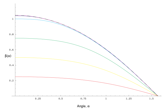
Figure 1: Plots of the function $\beta(\alpha)$ against $\alpha$ for of six different values of the initial data. The curves merge into a dashed enveloping curve that shows $\beta(\alpha)$ for the Pilch-Warner solution. For the Klebanov-Witten solution one has $\beta\equiv 0$.

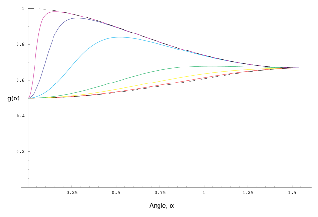
Figure 2: Plots of the function $g(\alpha)$ against $\alpha$ for of six different values of the initial data. The upper and lower dashed lines show the function, $g(\alpha)$, for the Pilch-Warner solution and for the Klebanov-Witten solution respectively. The horizontal dashed line shows the “target value”, ${2\over 3}$, for $g(\alpha)$ at $\alpha=\frac{\pi}{2}$.

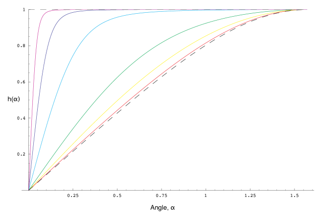
Figure 3: Plots of the function $h(\alpha)$ against $\alpha$ for of six different values of the initial data. The lower dashed curve shows $h(\alpha)$ for the Klebanov-Witten solution, while $h(\alpha)\equiv 1$ for the Pilch-Warner solution.

We have focussed on the set of regular solutions to the BPS equations. As we noted earlier, there is a three-parameter family of solutions in general. Our numerical solutions show that the other solutions to the BPS equations can be characterized as solutions starting from $g={1\over 2}$ at $\alpha=0$ and arriving at some arbitrary value of $g$ at $\alpha={\pi\over 2}$. The absence of conical singularities required that $(3g-1)\in{\mathbb{Z}}$, and the Klebanov-Witten solution imposed $(3g-1)=1$. However, there might be other interesting solutions to our BPS equations that are regular geometries but with different asymptotic values of $g$.

8 The central charge

As a final check on our results, we calculate the central charge of the family of solutions. It turns out that this is actually an exact calculation even though the exact solutions are not known. The central charge of the holographic dual gauge theory is proportional to the effective five-dimensional Newton constant [24, 20].

8.1 Calculating the effective five-dimensional Newton constant

The effective five-dimensional Newton constant $G_{5}$ is given by

$$G_{5}=G_{10}\int\limits_{X_{5}}\frac{1}{\Omega^{2}}\,e^{1}\wedge e^{2}\wedge e^{3}\wedge e^{4}\wedge e^{5}$$ (8.1)

Using the vielbein Ansatz this can be reduced to

$$G_{5}=2(2\pi)^{3}G_{10}\int\limits_{I}\frac{A_{1}A_{2}A_{3}A_{4}A_{5}}{\Omega^{2}}\,d\theta$$ (8.2)

Using the equations (6.17), (6.22) one can show that

$$G_{5}=-\frac{2(2\pi)^{3}G_{10}}{3}\int\limits_{I}(A_{1}^{2}A_{2}^{2})^{\prime}\,d\theta.$$ (8.3)

For the family of ${\cal N}=1$ theories the boundary conditions imply that

$$G_{5}^{(IR)}=\frac{2(2\pi)^{3}G_{10}f_{0}^{2}}{27},$$ (8.4)

whereas for the ${\cal N}=2$ theory

$$G_{5}^{(UV)}=\frac{3(2\pi)^{3}G_{10}f_{0}^{2}}{48}.$$ (8.5)

Note that the factor 3 in the enumerator is due to the different periodicity of $\phi$ as discussed in section 7.5. These formulas depend on the integration constant, $f_{0}$. This constant was introduced as the coefficient of the five-form flux. For this reason it is related to the number $N_{D3}$ of D3-branes, which is the rank of the gauge group. However, (8.4) already shows that the central charge of the dual field theory is constant across the entire family of solutions, and independent of the choice of the initial data for the BPS equations. To conclude that this implies that the central charge of the dual field theory is constant across the family one really needs to show that the parameter, $f_{0}$, represents the number of $D3$-branes present in the family of solutions. While this seems highly plausible, we will now prove it.

8.2 Calculating the rank of the gauge group

The Bianchi identity [22]

$$dF^{(5)}=\frac{i}{8}G\wedge G^{\ast}$$ (8.6)

implies that the five-form flux is not only sourced by D3-branes, but also by three-form flux. For this reason the total five-form flux cannot be used to determine the rank of the gauge group. The effect of the three-form flux can be subtracted as follows

$$N_{D3}=\int\limits_{X_{5}}\left(F^{(5)}-\frac{i}{16}\epsilon_{\alpha\beta}A^{\alpha}\wedge F^{\beta}\right).$$ (8.7)

The five-form under the integral is not gauge invariant by itself, but the integral is gauge invariant.

To determine this integral, we need to relate the quantities appearing here to metric and field coefficients. The internal part of the field strength $F^{(5)}$ is given by

$$F^{(5)}_{int}=\frac{f_{0}A_{1}A_{2}A_{3}A_{4}A_{5}}{\Omega^{10}}\,\sigma^{1}\wedge\sigma^{2}\wedge\sigma^{3}\wedge d\theta\wedge d\phi$$ (8.8)

The three-form flux $F^{(3)}=F^{1}=(F^{2})^{\ast}$ is related to $G$ by

$$G=-\epsilon_{\alpha\beta}V^{\alpha}_{+}\,F^{\beta}.$$ (8.9)

Using the identity

$$|V_{+}^{2}|^{2}-|V_{+}^{1}|^{2}=1,$$ (8.10)

the foregoing relation can be inverted to yield

$$F^{(3)}=V_{+}^{2}{}^{\ast}G+V^{1}_{+}G^{\ast}.$$ (8.11)

In our geometry $G$ has the form

$$\begin{array}[]{rl}G=&h_{1}\sigma^{1}\wedge\sigma^{3}\wedge d\theta+h_{2}\sigma^{2}\wedge\sigma^{3}\wedge d\theta+h_{3}\sigma^{1}\wedge\sigma^{3}\wedge d\phi+\\ +&h_{4}\sigma^{2}\wedge\sigma^{3}\wedge d\phi+h_{5}\sigma^{1}\wedge d\theta\wedge d\phi+h_{6}\sigma^{2}\wedge d\theta\wedge d\phi,\end{array}$$ (8.12)

which implies, that $F^{(3)}$ has the form

$$\begin{array}[]{rl}F^{(3)}&=f_{1}\sigma^{1}\wedge\sigma^{3}\wedge d\theta+f_{2}\sigma^{2}\wedge\sigma^{3}\wedge d\theta+f_{3}\sigma^{1}\wedge\sigma^{3}\wedge d\phi+\\ +&f_{4}\sigma^{2}\wedge\sigma^{3}\wedge d\phi+f_{5}\sigma^{1}\wedge d\theta\wedge d\phi+f_{6}\sigma^{2}\wedge d\theta\wedge d\phi.\end{array}$$ (8.13)

The field strength, $F^{(3)}$, satisfies the Bianchi identity $dF^{(3)}=0$, which implies

$$f_{5}=-f_{4}^{\prime}\qquad{\rm and}\qquad f_{6}=f_{3}^{\prime}.$$ (8.14)

A two-form potential $A^{(2)}$ for such an $F^{(3)}$ is then

$$A^{(2)}=-f_{1}\sigma^{2}\wedge d\theta+f_{2}\sigma^{1}\wedge d\theta-f_{3}\sigma^{2}\wedge d\phi+f_{4}\sigma^{1}\wedge d\phi.$$ (8.15)

This can be used to determine

$$\epsilon_{\alpha\beta}A^{\alpha}F^{\beta}=2(f_{1}f_{3}^{\ast}-f_{1}^{\ast}f_{3}+f_{2}f_{4}^{\ast}-f_{2}^{\ast}f_{4})\,\sigma^{1}\wedge\sigma^{2}\wedge\sigma^{3}\wedge d\theta\wedge d\phi$$ (8.16)

or

$$\epsilon_{\alpha\beta}A^{\alpha}F^{\beta}=2(h_{1}h_{3}^{\ast}-h_{1}^{\ast}h_{3}+h_{2}h_{4}^{\ast}-h_{2}^{\ast}h_{4})\,\sigma^{1}\wedge\sigma^{2}\wedge\sigma^{3}\wedge d\theta\wedge d\phi$$ (8.17)

This can be reexpressed in terms of the vielbein coefficients

$$\begin{array}[]{c}\epsilon_{\alpha\beta}A^{\alpha}F^{\beta}=\\ =-4A_{3}^{2}A_{4}A_{5}((g_{1}+g_{4})(g_{3}+g_{6})A_{1}^{2}+(g_{1}-g_{4})(g_{3}-g_{6})A_{2}^{2})\,\sigma^{1}\wedge\sigma^{2}\wedge\sigma^{3}\wedge d\theta\wedge d\phi\end{array}$$ (8.18)

One can check that

$$\begin{array}[]{l}-\frac{(A_{1}^{2}A_{2}^{2}\cos^{2}\beta)^{\prime}}{3f_{0}}=\\ \frac{f_{0}A_{1}A_{2}A_{3}A_{4}A_{5}}{\Omega^{10}}+\frac{iA_{3}^{2}A_{4}A_{5}((g_{1}+g_{4})(g_{3}+g_{6})A_{1}^{2}+(g_{1}-g_{4})(g_{3}-g_{6})A_{2}^{2})}{144}.\end{array}$$ (8.19)

which implies that

$$N_{D3}=-\frac{2(2\pi)^{3}}{3f_{0}}\int\limits_{I}(A_{1}^{2}A_{2}^{2}\cos^{2}\beta)^{\prime}\,d\theta.$$ (8.20)

For the family of ${\cal N}=1$ theories this yields:

$$N_{D3}^{(IR)}=\frac{2(2\pi)^{3}f_{0}}{27}$$ (8.21)

and for the ${\cal N}=2$ theory this is

$$N_{D3}^{(UV)}=\frac{3(2\pi)^{3}f_{0}}{48}.$$ (8.22)

This enables us to express the effective five-dimensional Newton constant in terms of the rank of the gauge group

$$G_{5}^{(IR)}=\frac{27G_{10}N_{D3}^{(IR)}{}^{2}}{2(2\pi)^{3}}\qquad{\rm and}\qquad G_{5}^{(UV)}=\frac{48G_{10}N_{D3}^{(IR)}{}^{2}}{3(2\pi)^{3}}.$$ (8.23)

The ratio of the effective five-dimensional Newton constants is exactly the ratio of the central charges of the UV and the IR gauge theories

$$\frac{G_{5}^{(IR)}}{G_{5}^{(UV)}}=\frac{27}{32}=\frac{c_{(IR)}}{c_{(UV)}}.$$ (8.24)

Thus the family of solutions has precisely the correct central charge to be the duals of the family of fixed points predicted in [3, 19].

9 Conclusions

We have found the long-sought family of $AdS_{5}$ vacuum solutions that interpolate between the $T^{1,1}$ compactification and the flux compactification of Pilch and Warner [4]. This family of solutions is holographically dual to the family of ${\cal N}=1^{*}$ IR fixed points that can be obtained by flowing from an ${\cal N}=2$, ${\mathbb{Z}}_{2}$ quiver gauge theory. In the field theory, this family is parametrized by the ratio, $m_{1}/m_{2}$, of masses given to the chiral multiplets on each node of the quiver. In supergravity the difference of the masses, $m_{1}-m_{2}$, is dual to the Kähler modulus of a non-trivial $S^{2}$, while the sum of the masses, $m_{1}+m_{2}$, is dual to a non-trivial, three-form field strength. Thus the family represents a kind of continuous geometric transition in which a Kähler deformation is traded for flux.

One of the surprises, and perhaps one of the reasons why this solution was not discovered earlier, is that the generic solution has a non-trivial dilaton. It is surprising because the dilaton background is trivial for the two previously know (KW and PW) solutions. There are obvious questions about whether there is any interesting physics to be learned from the non-trivial dilaton profiles. On the more mathematical side, it raises questions about the underlying geometric structure of these solutions. One of the important insights of [16] was that the geometry of the PW solution, and indeed the flows to and around it [7, 25], possessed an integrable complex structure, and indeed were “almost Calabi-Yau.” The non-trivial dilaton profile, and indeed the fact that it is real, seems to be at odds with the integrability of the complex structure. We have tried the obvious generalizations of the integrable complex structure found in [16] and they fail to work here, and this failure perhaps explains the incompatibility of the complex structures, noted in [25], of the PW flow and of the Calabi-Yau metric that must underlie [16] the KW flow. There is thus an interesting issue as to how to characterize the geometry of the interpolating family obtained here.

The system of BPS equations that we obtained were surprisingly complicated, also probably as a consequence of the non-trivial dilaton profile. This is all the more surprising in the light of the results of [3] that led to the conjectured existence of the family of solutions. It was shown in [3] that, from the perspective of five-dimensional, ${\cal N}=4$ gauged supergravity, all the vacuum solutions in the family, and indeed all the flows to them, were governed by exactly the same set of equations. The complete family, in five-dimensional supergravity, is swept out by the action of an $SU(2)$ symmetry. One would therefore, naively, expect an equally simple formulation in ten-dimensions. However, as was pointed out in [3], and as we see explicitly here, this sweeping out of the family involves some extremely non-trivial trading of very different geometric quantities in ten dimensions. It is certainly not the first time that a trivial symmetry in lower dimensions has led to subtle or profound effects in higher dimensions, and indeed the parallels between the present example and mirror symmetry are rather intriguing. It would certainly be very interesting to find how the symmetry that sweeps out the family acts in ten dimensions. This might be similar to the $SL(2,{\rm I\kern-1.79993ptR})$ action in [17]. For this reason there should be a simpler form of our BPS equations and a way to solve them analytically. However, in string theory such a continous symmetry group of the supergravity will be broken down to a discrete duality group by solitonic excitations [26, 27, 28].

There is also the issue of the flow solutions: We have found the fixed points, but it would be very useful to find the family of flows from the quiver gauge theories to these fixed points. Finding these might also shed light upon the underlying geometric structure.

As a final comment, we found the family of solutions by a very careful analysis of the symmetries of the field theory. In particular, the discrete ${\mathbb{Z}}_{2}$ symmetry in combination with the $SO(3)$ symmetry played a very significant role in fixing the metric Ansatz and in determining one of the supersymmetry projectors. We suspect that such a careful treatment of such discrete symmetries of will also give new insights into how to solve other open problems in holographic descriptions of field theories, especially for field theories related to ${\cal N}=4$ SYM.

Acknowledgments

This work is supported in part by funds provided by the DOE under grant number DE-FG03-84ER-40168. The work of NH is supported in part by a Fletcher Jones Graduate Fellowship from USC. Research at the Perimeter Institute is supported in part by funds from NSERC of Canada.

NH would like to thank the theory group at Stony Brook and ANU for hospitality. CR and NW would like to thank the Aspen Center for Physics in which part of the work was done.

We would like to thank Andy Brandhuber, Alex Buchel, Rich Corrado, Jerome Gauntlett, Jaume Gomis, Peter Mayr, Andrei Starinets and Nemani Suryanarayana for useful discussions.

Appendix A Some Clifford algebra

A.1 Generalities

The Clifford algebra is defined by the anticommutation relations

$$\{\gamma^{m},\gamma^{n}\}=2\eta^{mn},$$ (A.1)

where $\eta^{mn}=\eta^{m}\delta^{mn}$. We choose a representation in which $\sqrt{\eta^{m}}\gamma^{m}$ is Hermitean. Given a complex structure, one can define the raising and lowering operators

$$\Gamma^{m}=\sqrt{\eta^{2m-1}}\gamma^{2m-1}+i\sqrt{\eta^{2m}}\gamma^{2m},\quad{\rm and}\quad(\Gamma^{m})^{\dagger}=\sqrt{\eta^{2m-1}}\gamma^{2m-1}-i\sqrt{\eta^{2m}}\gamma^{2m}.$$ (A.2)

Then the raising and lowering operators satisfy the following anticommutation relations:

$$\{\Gamma^{m},\Gamma^{n}\}=\{(\Gamma^{m})^{\dagger},(\Gamma^{n})^{\dagger}\}=0\quad{\rm and}\quad\{\Gamma^{m},(\Gamma^{n})^{\dagger}\}=4\delta^{mn}.$$ (A.3)

One can then define the fermion number operators

$$F^{m}=i\sqrt{\eta^{2m-1}}\gamma^{2m-1}\sqrt{\eta^{2m}}\gamma^{2m}=1-{\frac{1}{2}}\Gamma^{m}(\Gamma^{m})^{\dagger}=-1+{\frac{1}{2}}(\Gamma^{m})^{\dagger}\Gamma^{m}.$$ (A.4)

The chirality operator is then the product of all the Fermion number operators $\gamma=F^{1}\cdots F^{n}$.

The Fermion number operators have eigenvalues $\pm 1$. The eigenvalues of the Fermion number operators can be used to label a basis of states. One can define a ground state $|0\rangle$ which is anihilated by all the lowering operators. It has Fermion number $-1$ for all Fermion number operators. All other states can be gotten by applying raising operators. If one labels a state by $|\nu_{1},\cdots,\nu_{n}\rangle$, then the raising and lowering operators act as follows:

$$|\nu_{1},\cdots,+1,\cdots,\nu_{n}\rangle = {\frac{1}{2}}\nu_{1}\cdots\nu_{m-1}(\Gamma^{m})^{\dagger}|\nu_{1},\cdots,-1,\cdots,\nu_{n}\rangle,$$ (A.5)

$$|\nu_{1},\cdots,-1,\cdots,\nu_{n}\rangle = {\frac{1}{2}}\nu_{1}\cdots\nu_{m-1}\Gamma^{m}|\nu_{1},\cdots,+1,\cdots,\nu_{n}\rangle.$$ (A.6)

This defines the matrix elements of the gamma matrices. One can see that in this basis $\Gamma^{m}$ is real. From this follows that

• The matrices $\sqrt{\eta^{m}}\gamma^{m}$ are Hermitean,

• The matrices $\sqrt{\eta^{2m-1}}\gamma^{2m-1}$ are symmetric and real and

• The matrices $\sqrt{\eta^{2m}}\gamma^{2m}$ are antisymmetric and imaginary.

In general there are matrices $B$, $C$ and $D$ such that

$$(\gamma^{m})^{*} = \eta_{B}B\gamma^{m}B^{-1},$$ (A.7)

$$(\gamma^{m})^{\dagger} = C\gamma^{m}C^{-1},$$ (A.8)

$$(\gamma^{m})^{t} = \eta_{B}D\gamma^{m}D^{-1},$$ (A.9)

where $\eta_{B}=\pm 1$ is a constant which is chosen (if possible) such that $BB^{*}=1$. One can see that $D=(B^{\dagger})^{-1}C$. Given a spinor $\epsilon$, $\epsilon^{\odot}=B^{-1}\epsilon^{*}$, $\bar{\epsilon}=\epsilon^{\dagger}C$ and $\tilde{\epsilon}=\epsilon^{t}D$ transform covariantly.

If $BB^{*}=1$ one can impose the Majorana condition $\epsilon=B^{-1}\epsilon^{*}$. And if $B$ commutes with the chirality operator $\gamma$, one can impose the Majorana-Weyl condition.

In the following we collect useful Gamma matrix identities in various dimensions.

A.2 $Spin(1,9)$

Chirality operator:

$$\gamma=-\gamma^{0\cdots 9}$$ (A.10)

Complex conjugation:

$$B=\gamma^{013579}$$ (A.11)

$$B\gamma^{M}B^{-1}=-(\gamma^{M})^{*}$$ (A.12)

$$B\gamma_{(10)}B^{-1}=\gamma_{(10)}^{*}$$ (A.13)

$$BB^{*}=1$$ (A.14)

Hermitean conjugation:

$$C=\gamma^{0}$$ (A.15)

$$C\gamma^{M}C^{-1}=(\gamma^{M})^{\dagger}$$ (A.16)

Transpose:

$$D=(B^{\dagger})^{-1}\,C=-\gamma^{13579}$$ (A.17)

$$D\gamma^{M}D^{-1}=-(\gamma^{M})^{t}$$ (A.18)

A.3 $Spin(1,4)$

Chirality operator:

$$\gamma^{4}=-\gamma^{0123}$$ (A.19)

$$\gamma^{01234}=1$$ (A.20)

Complex Conjugation:

$$B=\gamma^{013}$$ (A.21)

$$B\gamma^{\mu}B^{-1}=(\gamma^{\mu})^{*}$$ (A.22)

$$BB^{*}=-1$$ (A.23)

Hermitean conjugation:

$$C=\gamma^{0}$$ (A.24)

$$C\gamma^{\mu}C^{-1}=(\gamma^{\mu})^{\dagger}$$ (A.25)

Transpose:

$$D=(B^{\dagger})^{-1}\,C=\gamma^{13}$$ (A.26)

$$D\gamma^{\mu}D^{-1}=(\gamma^{\mu})^{t}$$ (A.27)

A.4 $Spin(5)$

Chirality operator:

$$\gamma^{5}=-\gamma^{1234}$$ (A.28)

$$\gamma^{12345}=-1$$ (A.29)

Complex Conjugation:

$$B=\gamma^{24}$$ (A.30)

$$B\gamma^{m}B^{-1}=(\gamma^{m})^{*}$$ (A.31)

$$BB^{*}=-1$$ (A.32)

Hermitean conjugation:

$$C=1$$ (A.33)

$$C\gamma^{m}C^{-1}=(\gamma^{m})^{\dagger}$$ (A.34)

Transpose:

$$D=(B^{\dagger})^{-1}\,C=\gamma^{24}$$ (A.35)

$$D\gamma^{m}D^{-1}=(\gamma^{m})^{t}$$ (A.36)

It is easy to check that

$$\begin{array}[]{cc}B^{-1}|++\rangle^{*}=|--\rangle,&B^{-1}|+-\rangle^{*}=-|-+\rangle,\\ B^{-1}|-+\rangle^{*}=|+-\rangle,&B^{-1}|--\rangle^{*}=-|++\rangle.\end{array}$$ (A.37)

A.5 Decomposition of a ten-dimensional spinor

We want to decompose spinors in ten-dimensional Minkowski space of mostly minus signature into four-dimensional and six-dimensional spinors. The gamma matrices can be decomposed as

$$\gamma_{(10)}^{\mu}=\left(\begin{array}[]{cc}0&\gamma_{(e)}^{\mu}\otimes 1_{(i)}\\ \gamma_{(e)}^{\mu}\otimes 1_{(i)}&0\end{array}\right)\quad{\rm and}\quad\gamma_{(10)}^{m}=\left(\begin{array}[]{cc}0&-1_{(e)}\otimes\gamma_{(i)}^{m}\\ 1_{(e)}\otimes\gamma_{(i)}^{m}&0\end{array}\right).$$ (A.38)

Note that the internal gamma matrices $\gamma_{(i)}^{m}$ have a $+$-signaturte.

The ten-dimensional chirality operator is given by

$$\gamma_{(10)}=-\gamma_{(10)}^{0\cdots 9}=\left(\begin{array}[]{cc}1&0\\ 0&-1\end{array}\right),$$ (A.39)

the complex conjugation is given by

$$B_{(10)}=\left(\begin{array}[]{cc}B_{(e)}\otimes B_{(i)}&0\\ 0&-B_{(e)}\otimes B_{(i)}\end{array}\right)$$ (A.40)

and the hermitean conjugation is given by

$$C_{(10)}=\left(\begin{array}[]{cc}0&C_{(e)}\otimes C_{(i)}\\ C_{(e)}\otimes C_{(i)}&0\end{array}\right).$$ (A.41)

Appendix B The spin connection of the internal metric

The derivatives of the vielbein are

$$de^{1} = \frac{A_{1}^{\prime}}{A_{1}A_{4}}e^{4}\wedge e^{1}+\frac{A_{1}}{A_{2}A_{3}}e^{2}\wedge e^{3}-\frac{A_{1}B_{1}}{A_{2}A_{5}}e^{2}\wedge e^{5}-\frac{A_{1}B_{2}}{A_{2}A_{4}}e^{2}\wedge e^{4},$$ (B.1)

$$de^{2} = \frac{A_{2}^{\prime}}{A_{2}A_{4}}e^{4}\wedge e^{2}-\frac{A_{2}}{A_{1}A_{3}}e^{1}\wedge e^{3}+\frac{A_{2}B_{1}}{A_{1}A_{5}}e^{1}\wedge e^{5}+\frac{A_{2}B_{2}}{A_{1}A_{4}}e^{1}\wedge e^{4},$$ (B.2)

$$de^{3} = \frac{A_{3}^{\prime}}{A_{3}A_{4}}e^{4}\wedge e^{3}+\frac{A_{3}}{A_{1}A_{2}}e^{1}\wedge e^{2}+\frac{A_{3}B_{1}^{\prime}}{A_{4}A_{5}}e^{4}\wedge e^{5},$$ (B.3)

$$de^{4} = 0,$$ (B.4)

$$de^{5} = \frac{A_{5}^{\prime}}{A_{5}A_{4}}e^{4}\wedge e^{5}.$$ (B.5)

This leads to the following spin connection:

$$\omega_{114} = \frac{A_{1}^{\prime}}{A_{1}A_{4}},$$ (B.6)

$$\omega_{123} = -\frac{A_{1}}{2A_{2}A_{3}}+\frac{A_{2}}{2A_{1}A_{3}}+\frac{A_{3}}{2A_{1}A_{2}},$$ (B.7)

$$\omega_{124} = \frac{A_{1}B_{2}}{2A_{2}A_{4}}-\frac{A_{2}B_{2}}{2A_{1}A_{4}},$$ (B.8)

$$\omega_{125} = \frac{A_{1}B_{1}}{2A_{2}A_{5}}-\frac{A_{2}B_{1}}{2A_{1}A_{5}},$$ (B.9)

$$\omega_{224} = \frac{A_{2}^{\prime}}{A_{2}A_{4}},$$ (B.10)

$$\omega_{213} = -\frac{A_{1}}{2A_{2}A_{3}}+\frac{A_{2}}{2A_{1}A_{3}}-\frac{A_{3}}{2A_{1}A_{2}},$$ (B.11)

$$\omega_{214} = \frac{A_{1}B_{2}}{2A_{2}A_{4}}-\frac{A_{2}B_{2}}{2A_{1}A_{4}},$$ (B.12)

$$\omega_{215} = \frac{A_{1}B_{1}}{2A_{2}A_{5}}-\frac{A_{2}B_{1}}{2A_{1}A_{5}},$$ (B.13)

$$\omega_{312} = \frac{A_{1}}{2A_{2}A_{3}}+\frac{A_{2}}{2A_{1}A_{3}}-\frac{A_{3}}{2A_{1}A_{2}},$$ (B.14)

$$\omega_{334} = \frac{A_{3}^{\prime}}{A_{3}A_{4}},$$ (B.15)

$$\omega_{345} = -\frac{A_{3}B_{1}^{\prime}}{2A_{4}A_{5}},$$ (B.16)

$$\omega_{412} = -\frac{A_{1}B_{2}}{2A_{2}A_{4}}-\frac{A_{2}B_{2}}{2A_{1}A_{4}},$$ (B.17)

$$\omega_{435} = -\frac{A_{3}B_{1}^{\prime}}{2A_{4}A_{5}},$$ (B.18)

$$\omega_{512} = -\frac{A_{1}B_{1}}{2A_{2}A_{5}}-\frac{A_{2}B_{1}}{2A_{1}A_{5}},$$ (B.19)

$$\omega_{534} = \frac{A_{3}B_{1}^{\prime}}{2A_{4}A_{5}},$$ (B.20)

$$\omega_{554} = \frac{A_{5}^{\prime}}{A_{5}A_{4}}.$$ (B.21)

Appendix C Recovering the fields

Going through all the independent BPS equations one can recover the vielbein coefficients from $\alpha$, $\beta$, $g$ and $h$

$$\Omega^{2} = \sqrt{\frac{f_{0}}{\cos\beta}},$$ (C.1)

$$A_{1} = \sqrt{-\frac{f_{0}\sin^{3}\alpha\,\sin\beta\,g(h^{2}+1)}{4\beta^{\prime}\cos\alpha}},$$ (C.2)

$$A_{2} = \sqrt{-\frac{f_{0}\sin^{3}\alpha\,\sin\beta\,g(h^{2}+1)}{4\beta^{\prime}\cos\alpha\,h^{2}}},$$ (C.3)

$$A_{3} = -\frac{\sqrt{f_{0}\cos\beta}\sin^{2}\alpha\,\sin\beta\,g(h^{2}+1)}{2\beta^{\prime}\cos\alpha\,h},$$ (C.4)

$$A_{4} = g\sqrt{\frac{f_{0}}{\cos\beta}},$$ (C.5)

$$A_{5} = -\frac{2}{3}\sqrt{\frac{f_{0}}{\cos\beta}}\cos\alpha,$$ (C.6)

$$B_{1} = \frac{4\beta^{\prime}\cos\alpha\,h}{3g\sin\alpha\,\sin\beta\,(h^{2}+1)},$$ (C.7)

$$p = -\frac{\beta^{\prime}\sin\beta\,(h^{2}-1)}{2\sqrt{f_{0}\cos\beta}\,g(h^{2}+1)},$$ (C.8)

$$g_{1} = \frac{\cos\beta\,\beta^{\prime}}{f_{0}g},$$ (C.9)

$$g_{2} = -\frac{4\sin\beta\,\cos\beta}{f_{0}}-\frac{\cot\alpha\,\beta^{\prime}}{f_{0}g},$$ (C.10)

$$g_{3} = -\frac{i\beta^{\prime}}{f_{0}g\sin\alpha},$$ (C.11)

$$g_{4} = \frac{\cos\beta\,\beta^{\prime}(h^{2}-1)}{f_{0}g(h^{2}+1)},$$ (C.12)

$$g_{5} = -\frac{\beta^{\prime}\cot\alpha\,(h^{2}-1)}{f_{0}g(h^{2}+1)},$$ (C.13)

$$g_{6} = \frac{i\beta^{\prime}(h^{2}-1)}{f_{0}g\sin\alpha\,(h^{2}+1)}.$$ (C.14)

Appendix D The resolution of an $A_{1}$ singularity

The Eguchi-Hansen metric can be written as

$$ds^{2}=4r^{6}(a+r^{4})^{-\frac{5}{2}}(2a+r^{4})dr^{2}+(a+r^{4})^{-{\frac{1}{2}}}\left(\frac{r^{8}}{2a+r^{4}}(\sigma^{1})^{2}+(2a+r^{4})((\sigma^{2})^{2}+(\sigma^{3})^{2})\right),$$ (D.1)

with $r\geq 0$. This is a global coordinate system which allows a smooth $a\rightarrow 0$ limit. A corresponding vielbein is

$$e^{1} = A_{1}\sigma^{1}=r^{4}(a+r^{4})^{-\frac{1}{4}}(2a+r^{4})^{-{\frac{1}{2}}}\sigma^{1},$$ (D.2)

$$e^{2} = A_{2}\sigma^{2}=(a+r^{4})^{-\frac{1}{4}}(2a+r^{4})^{\frac{1}{2}}\sigma^{2},$$ (D.3)

$$e^{3} = A_{3}\sigma^{3}=(a+r^{4})^{-\frac{1}{4}}(2a+r^{4})^{\frac{1}{2}}\sigma^{3},$$ (D.4)

$$e^{4} = A_{4}\sigma^{4}=2r^{3}(a+r^{4})^{-\frac{5}{4}}(2a+r^{4})^{\frac{1}{2}}dr.$$ (D.5)

The linearized perturbation around $a=0$ is given by

$$\delta A_{1} = -\frac{5}{4r^{3}}\delta a,$$ (D.6)

$$\delta A_{2}=\delta A_{3} = \frac{3}{4r^{3}}\delta a,$$ (D.7)

$$\delta A_{4} = \frac{1}{2r^{4}}\delta a$$ (D.8)

The size of the deformation can be determined using the natural metric

$$\delta g_{ij}\delta g_{kl}g^{ik}g^{jl}=\sqrt{A_{1}A_{2}A_{3}A_{4}}\,\sum_{i}\left(\frac{2\delta A_{i}}{A_{i}}\right)^{2}=\sqrt{2}r^{-\frac{13}{2}}\delta a^{2}.$$ (D.9)

This diverges as $r\rightarrow 0$, which indicates that the range of validity of the linearized approximation is smaller for small $r$.

References

- [1] J. M. Maldacena, “The large n limit of superconformal field theories and supergravity,” Adv. Theor. Math. Phys. 2 (1998) 231–252, hep-th/9711200.
- [2] E. Witten, “Anti-de sitter space and holography,” Adv. Theor. Math. Phys. 2 (1998) 253–291, hep-th/9802150.
- [3] R. Corrado, M. Gunaydin, N. P. Warner, and M. Zagermann, “Orbifolds and flows from gauged supergravity,” Phys. Rev. D65 (2002) 125024, hep-th/0203057.
- [4] K. Pilch and N. P. Warner, “A new supersymmetric compactification of chiral IIB supergravity,” Phys. Lett. B487 (2000) 22–29, hep-th/0002192.
- [5] L. J. Romans, “New Compactifications of Chiral N=2, d = 10 Supergravity,” Phys. Lett. B153 (1985) 392.
- [6] I. R. Klebanov and E. Witten, “Superconformal field theory on threebranes at a Calabi-Yau singularity,” Nucl. Phys. B536 (1998) 199–218, hep-th/9807080.
- [7] D. Z. Freedman, S. S. Gubser, K. Pilch, and N. P. Warner, “Renormalization group flows from holography supersymmetry and a c-theorem,” Adv. Theor. Math. Phys. 3 (1999) 363–417, hep-th/9904017.
- [8] A. Khavaev, K. Pilch, and N. P. Warner, “New vacua of gauged N = 8 supergravity in five dimensions,” Phys. Lett. B487 (2000) 14–21, hep-th/9812035.
- [9] R. G. Leigh and M. J. Strassler, “Exactly marginal operators and duality in four-dimensional N=1 supersymmetric gauge theory,” Nucl. Phys. B447 (1995) 95–136, hep-th/9503121.
- [10] J. P. Gauntlett, D. Martelli, J. Sparks, and D. Waldram, “Supersymmetric ads(5) solutions of m-theory,” Class. Quant. Grav. 21 (2004) 4335–4366, hep-th/0402153.
- [11] A. Butti, M. Grana, R. Minasian, M. Petrini, and A. Zaffaroni, “The baryonic branch of Klebanov-Strassler solution: A supersymmetric family of SU(3) structure backgrounds,” JHEP 03 (2005) 069, hep-th/0412187.
- [12] G. Dall’Agata, “On supersymmetric solutions of type IIB supergravity with general fluxes,” Nucl. Phys. B695 (2004) 243–266, hep-th/0403220.
- [13] C. N. Gowdigere, D. Nemeschansky, and N. P. Warner, “Supersymmetric solutions with fluxes from algebraic Killing spinors,” Adv. Theor. Math. Phys. 7 (2004) 787–806, hep-th/0306097.
- [14] K. Pilch and N. P. Warner, “Generalizing the N = 2 supersymmetric RG flow solution of IIB supergravity,” Nucl. Phys. B675 (2003) 99–121, hep-th/0306098.
- [15] K. Pilch and N. P. Warner, “N = 1 supersymmetric solutions of IIB supergravity from Killing spinors,” hep-th/0403005.
- [16] N. Halmagyi, K. Pilch, C. Römelsberger, and N. P. Warner, “The complex geometry of holographic flows of quiver gauge theories,” hep-th/0406147.
- [17] O. Lunin and J. Maldacena, “Deforming field theories with U(1) x U(1) global symmetry and their gravity duals,” JHEP 05 (2005) 033, hep-th/0502086.
- [18] M. R. Douglas and G. W. Moore, “D-branes, Quivers, and ALE Instantons,” hep-th/9603167.
- [19] R. Corrado and N. Halmagyi, “N = 1 field theories and fluxes in IIB string theory,” Phys. Rev. D71 (2005) 046001, hep-th/0401141.
- [20] S. S. Gubser, “Einstein manifolds and conformal field theories,” Phys. Rev. D59 (1999) 025006, hep-th/9807164.
- [21] D. Anselmi, D. Z. Freedman, M. T. Grisaru, and A. A. Johansen, “Nonperturbative formulas for central functions of supersymmetric gauge theories,” Nucl. Phys. B526 (1998) 543–571, hep-th/9708042.
- [22] J. H. Schwarz, “Covariant Field Equations of Chiral, N=2 D = 10 Supergravity,” Nucl. Phys. B226 (1983) 269.
- [23] P. Candelas and X. C. de la Ossa, “Comments on Conifolds,” Nucl. Phys. B342 (1990) 246–268.
- [24] M. Henningson and K. Skenderis, “The holographic Weyl anomaly,” JHEP 07 (1998) 023, hep-th/9806087.
- [25] C. N. Gowdigere and N. P. Warner, “Holographic Coulomb branch flows with N = 1 supersymmetry,” hep-th/0505019.
- [26] C. M. Hull and P. K. Townsend, “Unity of superstring dualities,” Nucl. Phys. B438 (1995) 109–137, hep-th/9410167.
- [27] E. Witten, “String theory dynamics in various dimensions,” Nucl. Phys. B443 (1995) 85–126, hep-th/9503124.
- [28] N. Halmagyi, C. Römelsberger, and N. P. Warner, “Inherited duality and quiver gauge theory,” hep-th/0406143.