Bulk versus Brane in the Absorption and Emission : $5$D Rotating Black Hole Case

Abstract

The absorption and emission spectra for the minimally-coupled brane and bulk scalar fields are numerically computed when the spacetime is a $5d$ rotating black hole carrying the two different angular momentum parameters $a$ and $b$. The effect of the superradiant scattering in the spectra is carefully examined. It is shown that the low-energy limit of the total absorption cross section always equal to the area of the non-spherically symmetric horizon, i.e. $4\pi(r_{H}^{2}+a^{2})$ for the brane scalar and $2\pi^{2}(r_{H}^{2}+a^{2})(r_{H}^{2}+b^{2})/r_{H}$ for the bulk scalar where $r_{H}$ is an horizon radius. The energy amplification for the bulk scalar is roughly order of $10^{-9}\%$ while that for the brane scalar is order of unity. This indicates that the effect of the superradiance is negligible for the case of the bulk scalar. Thus the standard claim that black holes radiate mainly on the brane is not changed although the effect of the superradiance is taken into account. The physical implication of this fact is discussed in the context of TeV-scale gravity.

The recent brane-world scenarios which assume the large[1, 2] or warped[3, 4] extra dimensions generally allow the emergence of the TeV-scale gravity, which opens the possibility to make the tiny black holes factory in the future high-energy colliders[5, 6, 7, 8, 9]. In this reason the absorption and emission problems for the higher-dimensional non-rotating black holes were extensively explored recently[10, 11, 12]. It was found[10] numerically that the emission on the brane is dominant compared to the emission off the brane in the Schwarzschild black hole background. This fact strongly supports the main conclusion of Ref.[13]. Adopting a different numerical technique used in Ref.[14, 15], it was also found[12] that the higher-dimensional charged black holes also radiate mainly on the brane if the number of the extra dimensions is not too large.

For the higher-dimensional rotating black holes, however, the situation can be more complicated. For the non-rotating black holes the crucial factor which makes the Hawking evaporation on the brane to be dominant is a geometrical factor $r_{H}/L<<1$, where $r_{H}$ is an horizon radius and $L$ is a size of the extra dimensions. In the rotating black holes, besides this geometrical factor, there is another important factor called superradiance, which means that the incident wave is amplified by the extraction of the rotation energy of the black holes under the particular condition. The effect of the superradiance in the $4d$ black holes was extensively studied long ago[16, 17, 18, 19]. The black hole bomb, i.e. rotating black hole plus mirror system, was recently re-examined in detail[20] from the aspect of the black hole stability.

The importance of the superradiance modes in the tiny rotating black holes produced by the high energy scattering in the future collider was discussed in Ref.[21, 22, 23]. Especially, in Ref.[23] it was shown that superradiance for the bulk scalar in the background of the $5d$ Myers-Perry rotating black hole[24] exists when the wave energy $\omega$ satisfies $0<\omega<m\Omega_{a}+k\Omega_{b}$, where $\Omega_{a}$ and $\Omega_{b}$ are angular frequencies of the black hole and, $m$ and $k$ are the azimuthal quantum numbers of the incident scalar wave. The generic conditions for the existence of the superradiance modes in the presence of single or multiple angular momentum parameters were derived recently[25, 26] when the incident bulk scalar, bulk electromagnetic and bulk gravitational waves are scattered by the higher-dimensional rotating black hole.

Recently, the emission spectra for the brane fields were explored analytically[27] in the low-energy regime and numerically[28, 29] in the entire range of the energy. The crucial difference of the brane fields from the bulk fields is the fact that the condition for the existence of the superradiance for the brane fields is $0<\omega<m\Omega$ while same condition for the bulk field is $0<\omega<\sum_{i}m_{i}\Omega_{i}$ as shown in Ref.[26]. Thus, in the background of the higher-dimensional black holes carrying the multiple angular momentum parameters the bulk field can be scattered superradiantly in the more wide range of $\omega$ compared to the brane fields. This may change the standard claim that black holes radiate mainly on the brane[13]. The purpose of this paper is to explore this issue by choosing the $5d$ Myers-Perry rotating black hole with two angular momentum parameters $a$ and $b$ as a prototype.

In the following we will compute the absorption and emission spectra in the full range of $\omega$ for the brane scalar and bulk scalar. As a computational technique we will adopt an appropriate numerical technique which will be explained in detail later. Although the superradiant scattering takes place more readily for the bulk scalar, its energy amplification arising due to the superradiance is shown to be roughly $10^{-9}\%$ while that for the brane scalar is order of unity. This fact indicates that the effect of the superradiance does not change the standard claim, i.e. black holes radiate mainly on the brane. In order to compare the superradiant effects in $4d$ and $5d$, we carry out the calculation in the Appendix for the superradiant scattering in the $4d$ Kerr background. The comparision reveals a big difference ($8$ orders of magnitude) for the energy amplification.

The $5d$ rotating black hole derived by Myers and Perry is expressed by a metric

$$ds_{5}^{2} = -dt^{2}+\frac{r^{2}\rho^{2}}{\bigtriangleup}dr^{2}+\rho^{2}d\theta^{2}+(r^{2}+a^{2})\sin^{2}\theta d\phi^{2}+(r^{2}+b^{2})\cos^{2}\theta d\psi^{2}$$ (2)

$$\hskip 56.9055pt+\frac{r_{0}^{2}}{\rho^{2}}(dt+a\sin^{2}\theta d\phi+b\cos^{2}\theta d\psi)^{2}$$

where $0\leq\phi,\psi<2\pi$, $0\leq\theta\leq\pi/2$,

$$\rho^{2} = r^{2}+a^{2}\cos^{2}\theta+b^{2}\sin^{2}\theta$$ (3)

$$\bigtriangleup = (r^{2}+a^{2})(r^{2}+b^{2})-r_{0}^{2}r^{2}$$ (4)

and, $a$ and $b$ are two angular momentum parameters. The mass $M$, two angular momenta $J_{1}$ and $J_{2}$ and the Hawking temperature $T_{H}$ are given by

$$M=\frac{3\pi r_{0}^{2}}{8}\hskip 28.45274ptJ_{1}=\frac{2}{3}Ma\hskip 28.45274ptJ_{2}=\frac{2}{3}Mb\hskip 28.45274ptT_{H}=\frac{r_{H}^{4}-a^{2}b^{2}}{2\pi r_{H}(r_{H}^{2}+a^{2})(r_{H}^{2}+b^{2})}$$ (5)

where $r_{H}$ is an horizon radius defined by $\bigtriangleup=0$ at $r=r_{H}$.

The induced $4d$ metric on the brane can be written as

$$ds_{4}^{2}=-dt^{2}+\frac{r^{2}\rho^{2}}{\bigtriangleup}dr^{2}+\rho^{2}d\theta^{2}+(r^{2}+a^{2})\sin^{2}\theta d\phi^{2}+\frac{r_{0}^{2}}{\rho^{2}}(dt+a\sin^{2}\theta d\phi)^{2}$$ (6)

if the self-gravity on the brane is negligible, where we assume $0\leq\theta\leq\pi$ to cover the whole $4d$ spacetime. The scalar wave equation $\Box\Phi_{BR}=0$ in the background (6) is not separable. If, however, $b=0$, this wave equation is separable into the following radial and angular equations:

$$\frac{d}{dr}\left(\tilde{\bigtriangleup}\frac{dR_{BR}}{dr}\right)+\left[\frac{[\omega(r^{2}+a^{2})-am]^{2}}{\tilde{\bigtriangleup}}-\Lambda_{\ell}^{m}\right]R_{BR}=0$$ (7)

$$\frac{1}{\sin\theta}\frac{d}{d\theta}\left(\sin\theta\frac{d\Theta_{BR}}{d\theta}\right)+\left[-\frac{m^{2}}{\sin^{2}\theta}+\omega^{2}a^{2}\cos^{2}\theta+{\cal E}_{\ell}^{m}\right]\Theta_{BR}=0$$ (8)

where $\tilde{\bigtriangleup}=r^{2}+a^{2}-r_{0}^{2}$ and $\Lambda_{\ell}^{m}={\cal E}_{\ell}^{m}+a^{2}\omega^{2}-2am\omega$. When deriving Eq.(7), we used a factorization condition $\Phi_{BR}=e^{-i\omega t}e^{-im\phi}R_{BR}(r)\Theta_{BR}(\theta)$.

The eigenvalue of the angular equation ${\cal E}_{\ell}^{m}$ was computed in Ref.[30] as an expansion of $a\omega$. Since, however, we need ${\cal E}_{\ell}^{m}$ when $a\omega$ is arbitrarily large, we would like to solve the angular equation numerically. This is easily solved as following. First, we note that $\Theta_{BR}$ becomes the usual spherical harmonics $|\ell,m>$ when $a\omega=0$. Of course, in this case ${\cal E}_{\ell}^{m}=\ell(\ell+1)$. When $a\omega\neq 0$, we expand $\Theta_{BR}$ as $\Theta_{BR}=\sum_{\ell^{\prime}}C_{\ell\ell^{\prime}}|\ell^{\prime},m>$. Then the angular equation reduces to the following eigenvalue equation

$$\sum_{\ell^{\prime}}A_{\ell^{\prime\prime}\ell^{\prime}}^{m}C_{\ell\ell^{\prime}}={\cal E}_{\ell}^{m}C_{\ell\ell^{\prime\prime}}$$ (9)

where

$$A_{\ell^{\prime\prime}\ell^{\prime}}^{m}=\ell^{\prime}(\ell^{\prime}+1)\delta_{\ell^{\prime}\ell^{\prime\prime}}-a^{2}\omega^{2}<\ell^{\prime\prime},m|\cos^{2}\theta|\ell^{\prime},m>.$$ (10)

Thus, the coefficients $C_{\ell\ell^{\prime}}$ and the separation constant ${\cal E}_{\ell}^{m}$ are simultaneously obtained by computing the eigenvectors and eigenvalues of the matrix $A_{\ell^{\prime\prime}\ell^{\prime}}^{m}$. Solving the eigenvalue equation (9) numerically, one can easily compute the $a\omega$-dependence of ${\cal E}_{\ell}^{m}$.

Now, we consider the wave equation $\Box\Phi_{BL}=0$ for the bulk scalar in the background of the $5d$ metric (2). The wave equation is always separable and the radial and angular equations are

$$\hskip 142.26378pt\frac{\bigtriangleup}{r}\frac{d}{dr}\left(\frac{\bigtriangleup}{r}\frac{R_{BL}}{dr}\right)+WR_{BL}=0$$ (11)

$$\frac{d}{d\theta}\left(\sin\theta\cos\theta\frac{d\Theta_{BL}}{d\theta}\right)+\left[\lambda_{\ell}^{m_{1}m_{2}}-\omega^{2}(a^{2}\sin^{2}\theta+b^{2}\cos^{2}\theta)-\frac{m_{1}^{2}}{\sin^{2}\theta}-\frac{m_{2}^{2}}{\cos^{2}\theta}\right]\sin\theta\cos\theta\Theta_{BL}=0$$ (12)

where

$$W=\bigtriangleup\left[-\lambda_{\ell}^{m_{1}m_{2}}+\omega^{2}(r^{2}+a^{2}+b^{2})+\frac{m_{1}^{2}(a^{2}-b^{2})}{r^{2}+a^{2}}+\frac{m_{2}^{2}(b^{2}-a^{2})}{r^{2}+b^{2}}\right]$$ (13)

$$\hskip 85.35826pt+r_{0}^{2}(r^{2}+a^{2})(r^{2}+b^{2})\left(\omega-\frac{m_{1}a}{r^{2}+a^{2}}-\frac{m_{2}b}{r^{2}+b^{2}}\right)^{2}.$$ (14)

When deriving Eq.(11), a factorization condition $\Phi_{BL}=e^{-i\omega t}e^{-i(m_{1}\phi+m_{2}\psi})R_{BL}(r)\Theta_{BL}(\theta)$ is used.

The angular equation can be solved numerically in a similar way to the case of the brane field. When $a=b=0$, the eigenfunction of the angular equation is expressed in terms of the Jacobi’s polynomial as following[23]

$$\Theta_{BL}\equiv|\ell,m_{1},m_{2}>=2^{-(m_{1}+m_{2}-1)/2}\sqrt{\frac{(2\ell+m_{1}+m_{2}+1)\Gamma[\ell+1]\Gamma[\ell+m_{1}+m_{2}+1]}{\Gamma[\ell+m_{1}+1]\Gamma[\ell+m_{2}+1]}}$$ (15)

$$\hskip 142.26378pt\times(1-\cos 2\theta)^{m_{1}/2}(1+\cos 2\theta)^{m_{2}/2}P_{\ell}^{(m_{1},m_{2})}(\cos 2\theta)$$ (16)

with $\lambda_{\ell}^{m_{1}m_{2}}=(2\ell+m_{1}+m_{2})(2\ell+m_{1}+m_{2}+2)$, where $P_{\ell}^{(m_{1},m_{2})}$ is a jacobi’s polynomial. When $a$ and $b$ are nonzero, we expand $\Theta_{BL}$ as $\Theta_{BL}=\sum_{\ell^{\prime}}D_{\ell\ell^{\prime}}|\ell^{\prime},m_{1},m_{2}>$. Then, by the same way as the brane case the angular equation reduces to the eigenvalue problem:

$$\sum_{\ell^{\prime}}B_{\ell^{\prime\prime}\ell^{\prime}}^{m_{1}m_{2}}D_{\ell\ell^{\prime}}=\lambda_{\ell}^{m_{1}m_{2}}D_{\ell\ell^{\prime\prime}}$$ (17)

where

$$B_{\ell^{\prime\prime}\ell^{\prime}}^{m_{1}m_{2}}=(2\ell^{\prime}+m_{1}+m_{2})(2\ell^{\prime}+m_{1}+m_{2}+2)\delta_{\ell^{\prime}\ell^{\prime\prime}}+<\ell^{\prime\prime},m_{1},m_{2}|\hat{H}_{1}|\ell^{\prime},m_{1},m_{2}>$$ (18)

with $\hat{H}_{1}=a^{2}\omega^{2}\sin^{2}\theta+b^{2}\omega^{2}\cos^{2}\theta$. Solving the eigenvalue equation (17) numerically, one can compute $\lambda_{\ell}^{m_{1}m_{2}}$.

Now, we would like to discuss how to solve the radial equations in (7) and (11). If we define $x=\omega r$ and $x_{H}=\omega r_{H}$, the radial equations reduce to

$$(x^{2}-x_{H}^{2})\frac{d}{dx}(x^{2}-x_{H}^{2})\frac{dR_{BR}}{dx}+\left[(x^{2}+a^{2}\omega^{2}-am\omega)^{2}-\Lambda_{\ell}^{m}(x^{2}-x_{H}^{2})\right]R_{BR}=0$$ (19)

$$\hskip 85.35826ptf(x,x_{H})\frac{d}{dx}f(x,x_{H})\frac{dR_{BL}}{dx}+\omega^{4}WR_{BL}=0$$ (20)

where

$$f(x,x_{H})=\frac{\omega^{4}\bigtriangleup}{x}=\frac{x_{H}^{2}(x^{2}+a^{2}\omega^{2})(x^{2}+b^{2}\omega^{2})-x^{2}(x_{H}^{2}+a^{2}\omega^{2})(x_{H}^{2}+b^{2}\omega^{2})}{xx_{H}^{2}}.$$ (21)

The radial equations (19) imply that if $R$ is a solution, $R^{\ast}$ is a solution too. The Wronskians between them become

$$W[R_{BR}^{\ast},R_{BR}]_{x}\equiv R_{BR}^{\ast}\frac{dR_{BR}}{dx}-R_{BR}\frac{dR_{BR}^{\ast}}{dx}=\frac{{\cal C}_{1}}{x^{2}-x_{H}^{2}}$$ (22)

$$W[R_{BL}^{\ast},R_{BL}]_{x}\equiv R_{BL}^{\ast}\frac{dR_{BL}}{dx}-R_{BL}\frac{dR_{BL}^{\ast}}{dx}=\frac{{\cal C}_{2}x}{(x^{2}-x_{H}^{2})(x^{2}-a^{2}b^{2}\omega^{4}/x_{H}^{2})}$$ (23)

where ${\cal C}_{1}$ and ${\cal C}_{2}$ are integration constants.

From the radial equations (19) one can derive the near-horizon and asymptotic solutions analytically as a series form[14, 15]. The explicit expressions for the solutions of the radial equations convergent near horizon are

$${\cal G}_{\ell,BR}^{m}(x,x_{H})=e^{\rho_{4}\ln|x-x_{H}|}\sum_{n=0}^{\infty}d_{\ell,n}^{m}(x-x_{H})^{n}$$ (24)

$${\cal G}_{\ell,BL}^{(m_{1},m_{2})}(x,x_{H})=e^{\rho_{5}\ln|x-x_{H}|}\sum_{n=0}^{\infty}d_{\ell,n}^{(m_{1},m_{2})}(x-x_{H})^{n}$$ (25)

where

$$\rho_{4}=-i\frac{\omega(r_{H}^{2}+a^{2})(\omega-m\Omega_{a})}{2x_{H}}\hskip 28.45274pt\rho_{5}=-i\frac{r_{H}(r_{H}^{2}+a^{2})(r_{H}^{2}+b^{2})(\omega-m_{1}\Omega_{a}-m_{2}\Omega_{b})}{2(r_{H}^{4}-a^{2}b^{2})}.$$ (26)

In Eq.(24) we choosed the sign in the exponents so that the solutions (24) become ingoing in the frame of reference of an observer co-rotating with a black hole. In Eq.(26) $\Omega_{a}$ and $\Omega_{b}$ are the angular frequency of the rotating black hole corresponding to the angular momentum parameters $a$ and $b$:

$$\Omega_{a}=\frac{a}{r_{H}^{2}+a^{2}}\hskip 56.9055pt\Omega_{b}=\frac{b}{r_{H}^{2}+b^{2}}.$$ (27)

The recursion relations for the coefficients $d_{\ell,n}^{m}$ and $d_{\ell,n}^{(m_{1},m_{2})}$ can be easily derived by inserting Eq.(24) into the radial equation (19). Since the explicit expressions are too lengthy, we will not present them. It is important to note that when $\omega<m\Omega_{a}$, the imaginary part of $\rho_{4}$ becomes positive. This implies that the near-horizon solution for the brane wave equation becomes the outgoing wave with respect to an observer at infinity. This guarantees that the superradiant scattering occurs at $0<\omega<m\Omega_{a}$ for the brane field. As expected, the second equation in Eq.(26) implies that the superradiance exists for the bulk scalar at $0<\omega<m_{1}\Omega_{a}+m_{2}\Omega_{b}$. Using Eq.(22) one can show that the Wronskians between the near-horizon solutions are

$$W[{\cal G}_{\ell,BR}^{m\ast},{\cal G}_{\ell,BR}^{m}]_{x}=-2i\omega\frac{(r_{H}^{2}+a^{2})(\omega-m\Omega_{a})}{x^{2}-x_{H}^{2}}|g_{\ell}^{m}|^{2}$$ (28)

$$W[{\cal G}_{\ell,BL}^{(m_{1},m_{2})\ast},{\cal G}_{\ell,BL}^{(m_{1},m_{2})}]_{x}=-2i\omega^{2}\frac{(r_{H}^{2}+a^{2})(r_{H}^{2}+b^{2})(\omega-m_{1}\Omega_{a}-m_{2}\Omega_{b})x}{r_{H}(x^{2}-x_{H}^{2})(x^{2}-a^{2}b^{2}\omega^{4}/x_{H}^{2})}|g_{\ell}^{(m_{1},m_{2})}|^{2}$$ (29)

where $g_{\ell}^{m}\equiv d_{\ell,0}^{m}$ and $g_{\ell}^{(m_{1},m_{2})}\equiv d_{\ell,0}^{(m_{1},m_{2})}$.

Next let us consider the solutions of the radial equations (19) convergent at the asymptotic regime:

$${\cal F}_{\ell(\pm),BR}^{m}(x,x_{H})=(\pm i)^{\ell+1}e^{\mp ix}(x-x_{H})^{\pm\rho_{4}}\sum_{n=0}^{\infty}\tau_{n(\pm)}^{BR}x^{-(n+1)}$$ (30)

$${\cal F}_{\ell(\pm),BL}^{(m_{1},m_{2})}(x,x_{H})=(\pm i)^{\ell+3/2}\frac{e^{\mp ix}(x-x_{H})^{\pm\rho_{5}}}{\sqrt{x}}\sum_{n=0}^{\infty}\tau_{n(\pm)}^{BL}x^{-(n+1)}.$$ (31)

${\cal F}_{(+)}$ and ${\cal F}_{(-)}$ represent the ingoing and outgoing waves respectively. The recursion relations between the coefficients are not explicitly given here. With an aid of Eq.(22) it is easy to show that the Wronskians between the asymptotic solutions are

$$W[{\cal F}_{\ell(+),BR}^{m},{\cal F}_{\ell(-),BR}^{m}]_{x}=\frac{2i}{x^{2}-x_{H}^{2}}$$ (32)

$$W[{\cal F}_{\ell(+),BL}^{(m_{1},m_{2})},{\cal F}_{\ell(-),BL}^{(m_{1},m_{2})}]_{x}=\frac{2ix}{(x^{2}-x_{H}^{2})(x^{2}-a^{2}b^{2}\omega^{4}/x_{H}^{2})}.$$ (33)

Next, we would like to show how the coefficients $g_{\ell}^{m}$ and $g_{\ell}^{(m_{1},m_{2})}$ are related to the partial scattering amplitude. For this we define the real scattering solutions $R_{\ell,BR}^{m}$ and $R_{\ell,BL}^{(m_{1},m_{2})}$, which behave as

$$R_{\ell,BR}^{m}\stackrel{{\scriptstyle x\rightarrow x_{H}}}{{\sim}}g_{\ell}^{m}(x-x_{H})^{\rho_{4}}[1+O(x-x_{H})]$$ (34)

$$R_{\ell,BL}^{(m_{1},m_{2})}\stackrel{{\scriptstyle x\rightarrow x_{H}}}{{\sim}}g_{\ell}^{(m_{1},m_{2})}(x-x_{H})^{\rho_{5}}[1+O(x-x_{H})]$$ (35)

$$R_{\ell,BR}^{m}\stackrel{{\scriptstyle x\rightarrow\infty}}{{\sim}}i^{\ell+1}\frac{2\ell+1}{2x}\left[e^{-ix+\rho_{4}\ln|x-x_{H}|}-(-1)^{\ell}S_{\ell}^{m}(x_{H})e^{ix-\rho_{4}\ln|x-x_{H}|}\right]+O(x^{-2})$$ (36)

$$R_{\ell,BL}^{(m_{1},m_{2})}\stackrel{{\scriptstyle x\rightarrow\infty}}{{\sim}}\sqrt{\frac{2}{\pi}}\frac{i^{\ell+3/2}(\ell+1)^{2}}{x^{3/2}}\left[e^{-ix+\rho_{5}\ln|x-x_{H}|}-(-1)^{\ell+1/2}S_{\ell}^{(m_{1},m_{2})}(x_{H})e^{ix-\rho_{5}\ln|x-x_{H}|}\right]+O(x^{-5/2})$$ (37)

where $S_{\ell}^{m}(x_{H})$ and $S_{\ell}^{(m_{1},m_{2})}(x_{H})$ are the scattering amplitudes for the brane and bulk scalars respectively. From the near-horizon behavior we can understand the Wronskians between the real scattering solutions $W[R_{\ell,BR}^{m\ast},R_{\ell,BR}^{m}]_{x}$ and $W[R_{\ell,BL}^{(m_{1},m_{2})\ast},R_{\ell,BL}^{(m_{1},m_{2})}]_{x}$ are exactly same with Eq.(28) respectively.

If we define the phase shifts $\delta_{\ell}^{m}(x_{H})=(1/2i)\ln S_{\ell}^{m}(x_{H})$ and $\delta_{\ell}^{(m_{1},m_{2})}(x_{H})=(1/2i)\ln S_{\ell}^{(m_{1},m_{2})}(x_{H})$, the asymptotic behavior of $R_{\ell,BR}^{m}$ and $R_{\ell,BL}^{(m_{1},m_{2})}$ can be written as

$$R_{\ell,BR}^{m}\stackrel{{\scriptstyle x\rightarrow\infty}}{{\sim}}\frac{2\ell+1}{x}e^{i\delta_{\ell}^{m}}\sin\left[x+i\rho_{4}\ln|x-x_{H}|-\frac{\pi\ell}{2}+\delta_{\ell}^{m}\right]+O(x^{-2})$$ (38)

$$R_{\ell,BL}^{(m_{1},m_{2})}\stackrel{{\scriptstyle x\rightarrow\infty}}{{\sim}}\sqrt{\frac{8}{\pi}}\frac{(\ell+1)^{2}}{x^{3/2}}e^{i\delta_{\ell}^{(m_{1},m_{2})}}\sin\left[x+i\rho_{5}\ln|x-x_{H}|-\pi\frac{\ell+1/2}{2}+\delta_{\ell}^{(m_{1},m_{2})}\right]+O(x^{-5/2}).$$ (39)

Assuming that the phase shifts are the complex quantities, i.e. $\delta_{\ell}^{m}\equiv\eta_{\ell}^{m}+i\beta_{\ell}^{m}$ and $\delta_{\ell}^{(m_{1},m_{2})}\equiv\eta_{\ell}^{(m_{1},m_{2})}+i\beta_{\ell}^{(m_{1},m_{2})}$, the Wronskians derived from the asymptotic behavior (38) are

$$W[R_{\ell,BR}^{m\ast},R_{\ell,BR}^{m}]_{x}=\frac{-i(2\ell+1)^{2}}{x^{2}-x_{H}^{2}}e^{-2\beta_{\ell}^{m}}\sinh 2\beta_{\ell}^{m}$$ (40)

$$W[R_{\ell,BL}^{(m_{1},m_{2})\ast},R_{\ell,BL}^{(m_{1},m_{2})}]_{x}=\frac{-8i(\ell+1)^{4}x}{\pi(x^{2}-x_{H}^{2})(x^{2}-a^{2}b^{2}\omega^{4}/x_{H}^{2})}e^{-2\beta_{\ell}^{(m_{1},m_{2})}}\sinh 2\beta_{\ell}^{(m_{1},m_{2})}.$$ (41)

Equating Eq.(40) with Eq.(28) yields

$$|g_{\ell}^{m}|^{2}=\frac{\left(\ell+\frac{1}{2}\right)^{2}}{\omega(r_{H}^{2}+a^{2})(\omega-m\Omega_{a})}(1-e^{-4\beta_{\ell}^{m}})$$ (42)

$$|g_{\ell}^{(m_{1},m_{2})}|^{2}=\frac{2(\ell+1)^{4}r_{H}}{\pi\omega^{2}(r_{H}^{2}+a^{2})(r_{H}^{2}+b^{2})(\omega-m_{1}\Omega_{a}-m_{2}\Omega_{b})}(1-e^{-4\beta_{\ell}^{(m_{1},m_{2})}}).$$ (43)

In the first equation of Eq.(42) $|g_{\ell}^{m}|^{2}>0$ implies that the greybody factor (or the transmission coefficient) $1-e^{-4\beta_{\ell}^{m}}\equiv 1-|S_{\ell}^{m}|^{2}$ becomes negative when $0<\omega<m\Omega_{a}$, which is nothing but the superradiant scattering. Similarly, the superradiance for the bulk scalar exists when $\omega$ satisfies $0<\omega<m_{1}\Omega_{a}+m_{2}\Omega_{b}$, which is easily deduced from the second equation of Eq.(42).

Now, we would like to discuss how to compute the physical quantities such as absorption cross section and emission rate from $g_{\ell}^{m}$ and $g_{\ell}^{(m_{1},m_{2})}$. For this discussion it is convenient to introduce new wave solutions $\tilde{R}_{\ell,BR}^{m}$ and $\tilde{R}_{\ell,BL}^{(m_{1},m_{2})}$, which differ from $R_{\ell,BR}^{m}$ and $R_{\ell,BL}^{(m_{1},m_{2})}$ in their normalization. They are normalized as

$$\tilde{R}_{\ell,BR}^{m}(x)\stackrel{{\scriptstyle x\rightarrow x_{H}}}{{\sim}}(x-x_{H})^{\rho_{4}}\left[1+O(x-x_{H})\right]$$ (44)

$$\tilde{R}_{\ell,BL}^{(m_{1},m_{2})}(x)\stackrel{{\scriptstyle x\rightarrow x_{H}}}{{\sim}}(x-x_{H})^{\rho_{5}}\left[1+O(x-x_{H})\right].$$ (45)

Since ${\cal F}_{(+)}$ and ${\cal F}_{(-)}$ derived in Eq.(30) are linearly independent solutions of the radial equations, we can gererally express these new wave solutions as a linear combination of ${\cal F}_{(\pm)}$:

$$\tilde{R}_{\ell,BR}^{m}=f_{\ell(-)}^{m}(x_{H}){\cal F}_{\ell(+),BR}^{m}(x,x_{H})+f_{\ell(+)}^{m}(x_{H}){\cal F}_{\ell(-),BR}^{m}(x,x_{H})$$ (46)

$$\tilde{R}_{\ell,BL}^{(m_{1},m_{2})}=f_{\ell(-)}^{(m_{1},m_{2})}(x_{H}){\cal F}_{\ell(+),BL}^{(m_{1},m_{2})}(x,x_{H})+f_{\ell(+)}^{(m_{1},m_{2})}(x_{H}){\cal F}_{\ell(-),BL}^{(m_{1},m_{2})}(x,x_{H})$$ (47)

where the coefficients $f_{\pm}$ are called the jost functions. Using Eq.(32) one can compute the jost functions in the following:

$$f_{\ell(\pm)}^{m}(x_{H})=\pm\frac{x^{2}-x_{H}^{2}}{2i}W[{\cal F}_{\ell(\pm),BR}^{m},\tilde{R}_{\ell,BR}^{m}]_{x}$$ (48)

$$f_{\ell(\pm)}^{(m_{1},m_{2})}(x_{H})=\pm\frac{(x^{2}-x_{H}^{2})(x^{2}-a^{2}b^{2}\omega^{4}/x_{H}^{2})}{2ix}W[{\cal F}_{\ell(\pm),BL}^{(m_{1},m_{2})},\tilde{R}_{\ell,BL}^{(m_{1},m_{2})}]_{x}.$$ (49)

Inserting the explicit expressions of ${\cal F}_{(\pm)}$ into Eq.(46) and comparing those with the asymptotic behavior of the real scattering solutions in Eq.(34), one can derive the following relations:

$$g_{\ell}^{m}(x_{H})=\frac{\ell+\frac{1}{2}}{f_{\ell(-)}^{m}(x_{H})},\hskip 28.45274ptS_{\ell}^{m}(x_{H})=\frac{f_{\ell(+)}^{m}(x_{H})}{f_{\ell(-)}^{m}(x_{H})}$$ (51)

$$g_{\ell}^{(m_{1},m_{2})}(x_{H})=\sqrt{\frac{2}{\pi}}\frac{(\ell+1)^{2}}{f_{\ell(-)}^{(m_{1},m_{2})}(x_{H})},\hskip 28.45274ptS_{\ell}^{(m_{1},m_{2})}(x_{H})=\frac{f_{\ell(+)}^{(m_{1},m_{2})}(x_{H})}{f_{\ell(-)}^{(m_{1},m_{2})}(x_{H})}.$$

Combining Eq.(42) and Eq.(51), we can compute the greybody factors in terms of the jost functions:

$${\cal T}_{\ell,BR}^{m}\equiv 1-|S_{\ell}^{m}|^{2}=\frac{\omega(r_{H}^{2}+a^{2})(\omega-m\Omega_{a})}{|f_{\ell(-)}^{m}|^{2}}$$ (52)

$${\cal T}_{\ell,BL}^{(m_{1},m_{2})}\equiv 1-|S_{\ell}^{(m_{1},m_{2})}|^{2}=\frac{\omega^{2}(r_{H}^{2}+a^{2})(r_{H}^{2}+b^{2})(\omega-m_{1}\Omega_{a}-m_{2}\Omega_{b})}{r_{H}|f_{\ell(-)}^{(m_{1},m_{2})}|^{2}}.$$ (53)

Thus if $0<\omega<m\Omega_{a}$, ${\cal T}_{\ell,BR}^{m}$ becomes negative which indicates the existence of the superradiance for the brane scalar. Same is true when $0<\omega<m_{1}\Omega_{a}+m_{2}\Omega_{b}$ for the bulk scalar.

The partial absorption cross section $\sigma_{\ell}^{m}$ for the brane scalar and $\sigma_{\ell}^{(m_{1},m_{2})}$ for the bulk scalar are given by

$$\sigma_{\ell}^{m}=\frac{\pi}{\omega^{2}}{\cal T}_{\ell,BR}^{m}=\frac{\pi(r_{H}^{2}+a^{2})(\omega-m\Omega_{a})}{\omega|f_{\ell(-)}^{m}|^{2}}$$ (54)

$$\sigma_{\ell}^{(m_{1},m_{2})}=\frac{4\pi}{\omega^{3}}{\cal T}_{\ell,BL}^{(m_{1},m_{2})}=\frac{4\pi(r_{H}^{2}+a^{2})(r_{H}^{2}+b^{2})(\omega-m_{1}\Omega_{a}-m_{2}\Omega_{b})}{x_{H}|f_{\ell(-)}^{(m_{1},m_{2})}|^{2}}.$$ (55)

Of course, the total absorption cross sections $\sigma_{BR}$ and $\sigma_{BL}$ are algebric sum of their partial absorption cross sections:

$$\sigma_{BR}=\sum_{\ell,m}\sigma_{\ell}^{m}\hskip 56.9055pt\sigma_{BL}=\sum_{\ell,m_{1},m_{2}}\sigma_{\ell}^{(m_{1},m_{2})}.$$ (56)

The total emission rate $\Gamma_{BR}$ for the brane scalar and $\Gamma_{BL}$ for the bulk scalar are given by

$$\Gamma_{BR}=\sum_{\ell,m}\Gamma_{\ell}^{m}d\omega\hskip 56.9055pt\Gamma_{BL}=\sum_{\ell,m_{1},m_{2}}\Gamma_{\ell}^{(m_{1},m_{2})}d\omega$$ (57)

where

$$\Gamma_{\ell}^{m}=\frac{1}{e^{(\omega-m\Omega_{a})/T_{H}}-1}\frac{\omega^{3}\sigma_{\ell}^{m}}{2\pi^{2}}$$ (58)

$$\Gamma_{\ell}^{(m_{1},m_{2})}=\frac{1}{e^{(\omega-m_{1}\Omega_{a}-m_{2}\Omega_{b})/T_{H}}-1}\frac{\omega^{4}\sigma_{\ell}^{(m_{1},m_{2})}}{8\pi^{2}}$$ (59)

and $T_{H}$ is an Hawking temperature given in Eq.(5). Therefore, we can compute all physical quantities related to the scattering between the rotating black hole and the scalar field if we can compute the jost functions.

Now, we would like to present briefly how to compute the jost functions numerically. It is important to note that besides the near-horizon or asymptotic solution, we can derive the solutions from the radial equations (19) which is convergent in the neighborhood of $x=b$, where $b$ is an arbitrary point. Their expressions are

$$\varphi_{\ell,BR}^{m}(x)=(x-x_{H})^{\rho_{4}}\sum_{n=0}^{\infty}D_{\ell,n}^{m}(x-b)^{n}$$ (60)

$$\varphi_{\ell,BL}^{(m_{1},m_{2})}(x)=(x-x_{H})^{\rho_{5}}\sum_{n=0}^{\infty}D_{\ell,n}^{(m_{1},m_{2})}(x-b)^{n}.$$ (61)

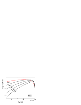
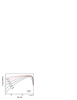
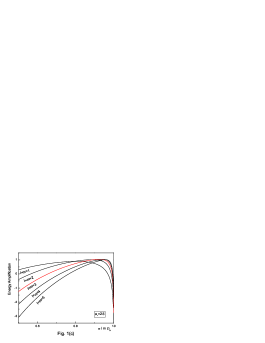
FIG. 1.: $Log$-plot of the energy amplification for the brane scalar when $a_{\ast}\equiv a/r_{H}$ is $1.5$ (Fig. 1(a)), $2.0$ (Fig. 1(b)), and $2.5$ (Fig. 1(c)). When $a_{\ast}=2.0$ (or $2.5$), the $\ell=m=2$ (or $\ell=m=3$) mode has a maximum peak. This means that the superradiant scattering of the higher modes becomes more and more significant when $a_{\ast}$ becomes larger. This seems to be the important effect of the extra dimensions.

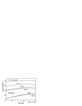
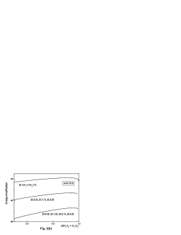
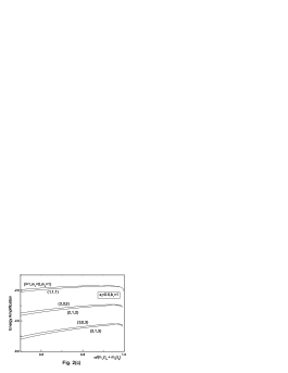
FIG. 2.: Energy amplification for the bulk scalar when $b_{\ast}\equiv b/r_{H}=0$ (Fig. 2(a)), $0.5$ (Fig. 2(b) and $1$ (Fig. 2(c)) with fixed $a_{\ast}$ as $0.5$. Usually the mode which satisfies $m_{1}+m_{2}=\ell$ has a maximum amplification at fixed $\ell$. Comparision with Fig. 1 leads a conclusion that the effect of the superradiance for the bulk scalar is negligible.

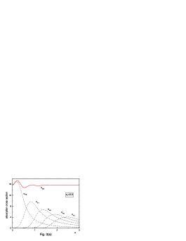
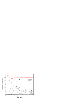
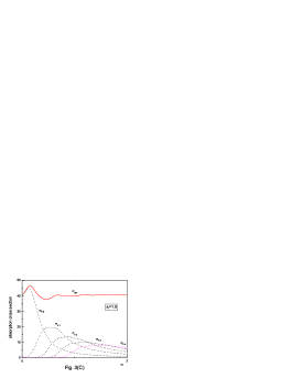
FIG. 3.: The total and partial absorption cross sections for the brane scalar when $a_{\ast}=0.5$ (Fig. 3(a), $1.0$ (Fig. 3(b)) and $1.5$ (Fig. 3(c)). Our numberical calculation shows that the low-energy limits of the total absorption cross sections always equal to the non-spherically symmetric horizon area $4\pi(r_{H}^{2}+a^{2})$. This fact gives rise to the conjecture that the universality for the scalar field discussed in Ref.[31] is extended to the non-spherically symmetric spacetime. In the high-energy limits they approach to the nonzero values which are roughly same with their low-energy limits.

The recursion relations between the coefficients can be explicitly derived by inserting Eq.(60) into the radial equation (19), which is not presented in this paper. Thus one can perform the matching procedure between the near-horizon and the asymptotic solutions by making use of this intermediate solutions as following. Matching procedure between the near-horizon solutions and $\varphi_{\ell}$ generates a solution whose domain of convergence is larger than the near-horizon region. Repeat of this matching procedure would increase the convergence region more and more. Similar matching procedure between the asymptotic solutions and $\varphi_{\ell}$ can be repeated to decrease the convergent region from the asymptotic region. Eventually, we can obtain two solutions which have common domain of convergence. Using these solutions we can compute the jost functions with an aid of Eq.(48).

Fig. 1 shows the $log$-plot of the superradiant scattering for the brane field. The $y$-axis is a $\ln(-100T_{\ell,BR}^{m})$ for the most favour modes. Fig. 1(a), (b), and (c) correspond to respectively $a_{\ast}=1.5$, $a_{\ast}=2.0$, and $a_{\ast}=2.5$ where $a_{\ast}\equiv a/r_{H}$. As commented in Ref.[28] the superradiant scattering for the higher modes becomes more and more significant as $a_{\ast}$ becomes larger. This fact is evidently verified in Fig. 1. Table I shows the first three modes at each $a_{\ast}$ whose maximum energy amplification is large. This Table shows that the lowest $\ell=m=1$ mode has a maximum energy amplification at $a_{\ast}=1.5$. But at $a_{\ast}=2.0$ (or $2.5$) $\ell=m=2$ (or $\ell=m=3$) mode has a maximum amplification. It also shows that the average amplification tends to increase with increasing $a_{\ast}$.

Table I: Maximum Energy Amplification for the Several Modes of Brane Scalar

Fig. 2 shows the $log$-plot of the superradiant scattering for the bulk scalar. The vertical axis is a $\ln(-100T_{\ell,BL}^{m_{1},m_{2}})$ when $b_{\ast}=0$, $0.5$ and $1$ with $a_{\ast}=0.5$ where $b_{\ast}\equiv b/r_{H}$. The modes in this figure are selected by comparing the maximum energy amplification at fixed $\ell$. Usually one of the mode which satisfies $m_{1}+m_{2}=\ell$ has the largest maximum amplification at given $\ell$. When, especially, $a_{\ast}=b_{\ast}$, the amplifications for the modes which have same $m_{1}+m_{2}$ are exactly identical. For example, when $\ell=2$, the amplications for $(0,2)$, $(1,1)$ and $(2,0)$ are exactly identical, where $(p,q)$ means $m_{1}=p$ and $m_{2}=q$. When $a\neq b$, this kind of degeneracy is broken. However, still one of the modes which satisfies $m_{1}+m_{2}=\ell$ generally has the largest maximum amplification. In Table II the maximum amplification values for several modes are given. Table I and Table II show that the energy amplification for the brane scalar is order of unity while that for the bulk scalar is order of $10^{-9}\%$ . This means that the effect of the superradiance for the bulk scalar is negligible. This indicates that consideration of the effect of the superradiance does not change the standard claim[13] that black holes radiate mainly on the brane. This will be confirmed in Fig. 5 explicitly.

Table II: Maximum Energy Amplification for the Several Modes of Bulk Scalar

Fig. 3 shows the total and partial absorption cross sections for the brane scalar when $a_{\ast}=0.5$, $1$ and $1.5$. The partial absorption cross section plotted in Fig. 3 is defined as $\sigma_{\ell}=\sum_{m}\sigma_{\ell}^{m}$. The negative value of $\sigma_{\ell}^{m}$ for $m>0$ in the range of $0<\omega<m\Omega_{a}$ arising due to the superradiant scattering is compensated by the positive value of $\sigma_{\ell}^{m}$ for $m\leq 0$ in the same range arising due to the normal scattering. Therefore, the partial absorption cross section $\sigma_{\ell}$ is positive in the full range of $\omega$.

FIG. 4.: The total absorption cross sections for the bulk scalar when $b_{\ast}=0$, $0.5$, and $1.0$ with $a_{\ast}=0.5$. The low-energy limits always equal to the area of the non-spherically symmetric horizon hypersurface $2\pi^{2}(r_{H}^{2}+a^{2})(r_{H}^{2}+b^{2})/r_{H}$. Unlike the non-rotating black hole the contribution of the higher partial waves to the total absorption cross section is negligible.

FIG. 5.: The total emission rate for the brane and bulk scalar fields. This figure shows that the $5d$ rotating black hole radiates mainly on the brane although we take the effect of the superradiance into account.

In the low-energy limits the total absorption cross sections exactly equal to the non-spherically symmetric horizon area ${\cal A}_{BR}$ defined

$${\cal A}_{BR}\equiv\int_{0}^{\pi}d\theta\int_{0}^{2\pi}d\phi\sqrt{g_{\theta\theta}g_{\phi\phi}-(g_{\theta\phi})^{2}}\Bigg{|}_{r=r_{H}}=4\pi(r_{H}^{2}+a^{2}).$$ (62)

As proved in Ref.[31] the low-energy limit of the total absorption cross section for the minimally coupled scalar always equals to the horizon area in the asymptotically flat and spherically symmetric black hole, which is called ‘universality’. Although the general proof is not given yet, our numerical investigation supports the evidence that this universality seems to be extended to the non-spherically symmetric background.

In the high-energy limits the total absorption cross sections approach to the nonzero values which are roughly same with the low-energy limits. In the intermediate region the total absorption cross sections do not exhibit an oscillatory pattern, which seems to be the effect of the extra dimensions[10, 12].

Fig. 4 shows the total absorption cross sections for the bulk scalar when $b_{\ast}=0$, $0.5$, and $1$ with $a_{\ast}=0.5$. The low-energy limits equal to the area of the non-spherically symmetric horizon hypersurface ${\cal A}_{BL}$ defined

$${\cal A}_{BL}\equiv\int_{0}^{\frac{\pi}{2}}d\theta\int_{0}^{2\pi}d\phi d\psi\sqrt{g_{\theta\theta}\left[g_{\phi\phi}g_{\psi\psi}-\left(g_{\phi\psi}\right)^{2}\right]}=2\pi^{2}\frac{(r_{H}^{2}+a^{2})(r_{H}^{2}+b^{2})}{r_{H}}.$$ (63)

This result also supports that the universality in Ref.[31] holds in the non-spherically symmetric background. In the high-energy limits the total absorption cross sections seem to approach to the nonzero values, which is much smaller than the low-energy limits. This fact indicates that unlike the non-rotating black hole case[10, 12], the contribution of the higher partial waves except S-wave to the total absorption cross section is too much negligible.

Fig. 5 shows the emission rate $\Gamma_{BL}/d\omega$ for the bulk scalar and $\Gamma_{BR}/d\omega$ for the brane scalar together. For the brane scalar we choosed $a=0.5$ and $b=0$ while for the bulk scalar $b$ is chosen as $0$, $0.5$ and $1$ with $a=0.5$. The wiggly pattern in $\Gamma_{BR}/d\omega$ indicates that unlike the non-rotating black holes the contribution of the higher partial waves is not negligible. This means that the effect of the superradiant scattering is crucially significant in the brane emission. This wiggly pattern disappears in $\Gamma_{BL}/d\omega$, which means that the effect of the superradiance is negligible. For the bulk scalar, therefore, the contribution of S-wave to the emission rate is dominant like the case of the non-rotating black hole background. Integrating the plots in Fig. 5, we can compute the total emission rate. For the brane scalar the total emission rate is $0.00353832$ and for the bulk scalar $0.000343955$, $0.000123524$ and $7.44114\times 10^{-6}$ for the cases of $b=0$, $b=0.5$ and $b=1$ respectively. Thus the emission rate for the bulk scalar is much smaller than that for the brane scalar. Thus the effect of the superradiance in $5d$ rotating black hole background does not seem to change the main conclusion of Ref.[13], i.e. black holes radiate mainly on the brane.

We computed the absorption and emission spectra for the brane and bulk scalar fields when the spacetime is an $5d$ rotating black hole carrying the two different angular momentum parameters. Although the effect of the superradiant scattering is taken into account, the main conclusion of Ref.[13] does not seem to be changed. This is due to the fact that the energy amplification for the bulk scalar is order of $10^{-9}\%$ while that for the brane scalar is order of unity. It seems to be straightforward to extend our calculation to the $6d$ rotating black hole background. It is of interest to check explicitly whether or not the effect of the superradiance is negligible in $6d$ case.

It is well-known that the Hawking radiation is highly dependent on the spin of the field. Thus, it seems to be greatly important to take the effect of spin into account in the higher-dimensional rotating black hole background. This is in progress and will be reported elsewhere.

Acknowledgement: This work was supported by the Korea Research Foundation under Grant (KRF-2003-015-C00109).

Appendix

The $4d$ Kerr metric is well-known in the form

$$ds^{2}= - (1-\frac{\mu r}{\Sigma})dt^{2}-\frac{2a\mu r\sin^{2}\theta}{\Sigma}dtd\phi+\frac{\Sigma}{\Delta}dr^{2}+\Sigma d\theta^{2}$$ (A.1)

$$+ (r^{2}+a^{2}+\frac{a^{2}\mu r\sin^{2}\theta}{\Sigma})\sin^{2}\theta d\phi^{2}$$ (A.2)

where $\Delta=r^{2}-\mu r+a^{2}\equiv(r-r_{+})(r-r_{-})$, $\Sigma=r^{2}+a^{2}\cos^{2}\theta$ and $r_{\pm}=(\mu\pm\sqrt{\mu^{2}-4a^{2}})/2$ are the inner and outer horizons. Then it is not difficult to show that the scalar wave equation $\Box\Phi=0$ in this background is separable. The radial and angular equations of this wave equation reduce to

$$\Delta\frac{d}{dr}\Delta\frac{dR}{dr}+[(r^{2}w+a^{2}w-am)^{2}-\Delta\Lambda_{\ell}^{m}]R=0$$ (A.3)

$$\frac{1}{\sin\theta}\frac{d}{d\theta}(\sin\theta\frac{dT}{d\theta})+[-\frac{m^{2}}{\sin^{2}\theta}+a^{2}w^{2}\cos^{2}\theta+E_{\ell}^{m}]T=0$$ (A.4)

where $\Phi=R(r)T(\theta)e^{im\phi}e^{-iwt}$, $\Lambda_{\ell}^{m}=E_{\ell}^{m}+a^{2}w^{2}-2amw$ and $E_{\ell}^{m}$ is a separation constant. Defining $x=wr$ and $x_{\pm}=wr_{\pm}$, one can show that the radial equation becomes

$$(x-x_{+})(x - x_{-})\frac{d}{dx}(x-x_{+})(x-x_{-})\frac{dR}{dx}$$ (A.5)

$$+ [(x^{2}+a^{2}w^{2}-amw)^{2}-\Lambda_{\ell}^{m}(x-x_{+})(x-x_{-})]R=0.$$ (A.6)

Solving the radial equation as a series form, one can derive the near-horizon solution

$${\cal G}_{\ell}^{m}(x,x_{+},x_{-})=e^{\lambda_{4}ln|x-x_{+}|}\sum_{n=0}^{\infty}d_{\ell,n}^{m}(x-x_{+})^{n}$$ (A.7)

and the asymptotic solution

$${\cal F}_{\ell(\pm)}^{m}(x,x_{+},x_{-})=(\pm i)^{\ell+1}e^{\mp ix}(x-x_{+})^{\pm\lambda_{4}}\sum_{n=0}^{\infty}\tau_{n(\pm)}x^{-(n+1)}$$ (A.8)

where the recursion relations for $d_{\ell,n}^{m}$ and $\tau_{n(\pm)}$ can be explicitly derived by inserting (A.7) and (A.8) into (A.5). The factor $\lambda_{4}$ arises due to the regular singular nature of the radial equation and its explicit expression is

$$\lambda_{4}=-i\frac{w(r_{+}^{2}+a^{2})(w-m\Omega)}{x_{+}-x_{-}}$$ (A.9)

where $\Omega=a/(r_{+}^{2}+a^{2})$ is an angular frequency of the black hole. If $0<w<m\Omega$, $Im\lambda_{4}$ becomes negative which indicates that the near-horizon solution (A.7) becomes outgoing wave. Thus the superradiant scattering takes place under the condition $0<w<m\Omega$.

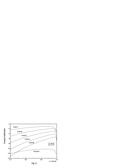
FIG. 6.: $Log$-plot of the energy amplification for the minimally-coupled scalar when the spacetime background is a $4d$ Kerr black hole with $a_{\ast}\equiv a/r_{+}=0.8$. This figure indicates that the energy amplification for the $4d$ case is order of $10^{-1}\%$ like the maximally rotating case.

The energy amplification arising due to the superradiant scattering was computed in Ref. [17, 28] when the spacetime background is a maximally rotating ($a_{\ast}\equiv a/r_{+}=1$) Kerr black hole. The authors in Ref. [17, 28] solved the radial and angular equations (A.3) directly by adopting the different numerical technique. For our case, however, the near-horizon and asymptotic solutions (A.7) and (A.8) are used. Thus our numerical method cannot be applied to the case of the maximally rotating black hole because $a_{\ast}=1$ implies the extremal limit, i.e. $r_{+}=r_{-}$ and $\lambda_{4}$ goes to infinity in this limit. Applying the numerical method used in the present paper the energy amplification can be straightforwardly computed for $a_{\ast}<1$.

Fig. 6 is a $\log$-plot of the energy amplification when $a_{\ast}=0.8$. Although Fig. 6 is different from Fig. 1 of Ref. [17] due to the different choice of $a_{\ast}$, it indicates that the energy amplification of the scalar wave in the $4d$ Kerr black hole is order of $10^{-1}\%$ like the case of $a_{\ast}=1$.

REFERENCES

[1] N. Arkani-Hamed, S. Dimopoulos and G. Dvali,
The Hierarchy Problem and New Dimensions at a Millimeter,
Phys. Lett. B429 (1998) 263 [hep-ph/9803315].
[2] L. Antoniadis, N. Arkani-Hamed, S. Dimopoulos and G. Dvali,
New Dimensions at a Millimeter to a Fermi and Superstrings at a
TeV, Phys. Lett. B436 (1998) 257 [hep-ph/9804398].
[3] L. Randall and R. Sundrum, A Large Mass Hierarchy from a
Small Extra Dimension,
Phys. Rev. Lett. 83 (1999) 3370 [hep-ph/9905221].
[4] L. Randall and R. Sundrum, An Alternative to
Compactification, Phys. Rev. Lett. 83 (1999) 4690 [hep-th/9906064].
[5] S. B. Giddings and T. Thomas, High energy colliders
as black hole factories: The end of short distance physics, Phys. Rev.
D65 (2002) 056010 [hep-ph/0106219].
[6] S. Dimopoulos and G. Landsberg, Black Holes at the
Large Hadron Collider, Phys. Rev. Lett. 87 (2001) 161602
[hep-ph/0106295].
[7] D. M. Eardley and S. B. Giddings, Classical black hole
production in high-energy collisions, Phys. Rev. D66 (2002)
044011 [gr-qc/0201034].
[8] D. Stojkovic, Distinguishing between the small ADD and
RS black holes in accelerators, Phys. Rev. Lett. 94 (2005)
011603 [hep-ph/0409124].
[9] V. Cardoso, E. Berti and M. Cavaglià, What we
(don’t) know about black hole formation in high-energy collisions
[hep-ph/0505125].
[10] C. M. Harris and P. Kanti, Hawking Radiation from a
-dimensional Black Hole: Exact Results for the Schwarzschild Phase,
JHEP 0310 (2003) 014 [hep-ph/0309054].
[11] E. Jung, S. H. Kim, and D. K. Park, Low-energy
absorption
cross section for massive scalar and Dirac fermion by -dimensional
Schwarzschild black hole, JHEP 0409 (2004) 005 [hep-th/0406117].
[12] E. Jung and D. K. Park, Absorption and Emission
Spectra of an higher-dimensional Reissner-Nordström black hole,
Nucl. Phys. B717 (2005) 272 [hep-th/0502002].
[13] R. Emparan, G. T. Horowitz and R. C. Myers, Black Holes
radiate mainly on the Brane, Phys. Rev. Lett. 85 (2000) 499
[hep-th/0003118].
[14] N. Sanchez, Absorption and emission spectra of a
Schwarzschild black hole, Phys. Rev. D18 (1978) 1030.
[15] E. Jung and D. K. Park, Effect of Scalar Mass in the
Absorption and Emission Spectra of Schwarzschild Black Hole, Class. Quant.
Grav. 21 (2004) 3717 [hep-th/0403251].
[16] Y. B. Zel’dovich, Generation of waves by a
rotating body, JETP Lett. 14 (1971) 180.
[17] W. H. Press and S. A. Teukolsky, Floating Orbits,
Superradiant Scattering and the Black-hole Bomb, Nature 238 (1972) 211.
[18] A. A. Starobinskii, Amplification of waves during
reflection from a rotating black hole, Sov. Phys. JETP 37 (1973)
28.
[19] A. A. Starobinskii and S. M. Churilov, Amplification
of electromagnetic and gravitational waves scattered by a rotating black
hole, Sov. Phys. JETP 38 (1974) 1.
[20] V. Cardoso, O. J. C. Dias, J. P. S. Lemos and S. Yoshida,
The black hole bomb and superradiant instabilities, Phys. Rev.
D70 (2004) 044039 [hep-th/0404096].
[21] V. Frolov and D. Stojković, Black hole radiation
in the brane world and the recoil effect, Phys. Rev. D66 (2002)
084002 [hep-th/0206046].
[22] V. Frolov and D. Stojković, Black Hole as a Point
Radiator and Recoil Effect on the Brane World, Phys. Rev. Lett.
89 (2002) 151302 [hep-th/0208102].
[23] V. Frolov and D. Stojković, Quantum radiation from
a -dimensional black hole, Phys. Rev. D67 (2003) 084004
[gr-qc/0211055].
[24] R. C. Myers and M. J. Perry, Black Holes in Higher
Dimensional Space-Times, Ann. Phys. 172 (1986) 304.
[25] E. Jung, S. H. Kim and D. K. Park, Condition for
Superradiance in Higher-dimensional Rotating Black Holes, Phys. Lett.
B615 (2005) 273
[hep-th/0503163].
[26] E. Jung, S. H. Kim and D. K. Park, Condition for the
Superradiance Modes in Higher-Dimensional Black Holes with Multiple
Angular Momentum Parameters [hep-th/0504139].
[27] D. Ida, K. Oda and S. C. Park, Rotating black holes
at future collider: Greybody factors for brane field, Phys. Rev.
D67 (2003) 064025 [hep-th/0212108].
[28] C. M. Harris and P. Kanti, Hawking Radiation from a
-Dimensional Rotating Black Hole [hep-th/0503010].
[29] D. Ida, K. Oda and S. C. Park, Rotating black holes
at future colliders II : Anisotropic scalar field emission [hep-th/0503052].
[30] E. Seidel, A comment on the eigenvalue of spin-weighted
spheroidal functions, Class. Quantum Grav. 6 (1989) 1057.
[31] S. R. Das, G. Gibbons, and S. D. Mathur,
Universality of Low Energy Absorption Cross Sections for Black Holes,
Phys. Rev. Lett. 78 (1997) 417 [hep-th/9609052].