Logarithmic corrections to the entropy of the exact string black hole

Abstract

Exploiting a recently constructed target space action for the exact string black hole, logarithmic corrections to the leading order entropy are studied. There are contributions from thermal fluctuations and from corrections due to $\alpha^{\prime}>0$ which for the microcanonical entropy appear with different signs and therefore may cancel each other, depending on the overall factor in front of the action. For the canonical entropy no such cancellation occurs. Remarks are made regarding the applicability of the approach and concerning the microstates. As a byproduct a formula for logarithmic entropy corrections in generic 2D dilaton gravity is derived.

1 Entropy of black holes

Entropy $S$ is a remarkable physical quantity and black holes with a horizon of area $A$ are remarkable (astro)physical objects. A full microscopical understanding of their combination, that is, the entropy of black holes (BHs), is often considered as an important mile stone on the road to quantum gravity. The famous Bekenstein–Hawking relation $S_{\mathrm{BH}}=A/4$ receives (to leading order logarithmic) corrections, $S=S_{\mathrm{BH}}+\alpha\ln{S_{\mathrm{BH}}}+\mathcal{O}(1)$ (with $\alpha=\mathrm{const.}$) from quantum gravity effects, but also from thermal fluctuations around the equilibrium. For a review on BH thermodynamics which discusses also logarithmic corrections to entropy cf. e.g. [1] and references therein. See [2] for further reviews.

The purpose of this paper is to discuss in detail the entropy of the exact string BH (ESBH) [3] and to calculate logarithmic corrections from thermal fluctuations as well as from subleading effects of the string-coupling $\alpha^{\prime}$. This is possible exploiting a target space action for the ESBH constructed recently [4]. The limitation of the current approach as well as the possibility of the cancellation of both contributions is discussed.

Probably because the corresponding calculations often are deceptively simple, there exists a large amount of literature devoted to the study of logarithmic corrections to entropy of various BHs, cf. [5, 6, 7, 8] (and references therein) for a somewhat randomly selected list of references. So the question arises whether it is useful and interesting to add yet another example. As to the usefulness, I attempt to clarify en passant some slightly confusing statements found in the literature regarding the applicability of calculations concerning thermal fluctuations, which may be of pedagogical value. Regarding the question of interest, the BH under consideration is the ESBH, a nonperturbative solution of 2D string theory, valid to all orders in $\alpha^{\prime}$. Until recently not even the leading order entropy could be calculated because no suitable target space action was known, but now that it is available one can easily obtain not only the leading order entropy but also logarithmic corrections to it. In particular, the intricate interplay between $\alpha^{\prime}$ corrections and thermal fluctuations will turn out to be of physical relevance.

As a byproduct a result for logarithmic corrections to entropy of generic 2D dilaton BHs is presented.

2 Logarithmic entropy corrections in generic 2D dilaton gravity

2.1 General features of thermal fluctuations

A brief collection of basic thermodynamical quantities with an explanation of our notation is contained in appendix A. The calculation of fluctuations below follows loosely [7], but differs in certain aspects. For a given mass $M$ sufficiently close to the equilibrium value $M_{0}$ one may expand the microcanonical entropy $S_{\rm mc}(M)=S_{\rm mc}(M_{0})+(M-M_{0})S^{\prime}_{\rm mc}+\frac{1}{2}\,(M-M_{0})^{2}S^{\prime\prime}_{\rm mc}+\dots$ perturbatively, where prime denotes differentiation with respect to mass and setting $M=M_{0}$ afterwards. Physically the BH mass is not fixed anymore but rather allowed to fluctuate around $M_{0}$, as expected for a BH coupled to a heat bath, e.g. provided by its own Hawking radiation. While the microcanonical entropy is a function of (fixed) mass, the canonical one depends on temperature and therefore is more suitable for our purposes. Temperature to leading order is given by $1/T=S^{\prime}_{\rm mc}$, which makes the integral in (35) a well-defined Gaussian one provided $S^{\prime\prime}_{\rm mc}<0$. Neglecting contributions of order of unity yields $S_{\rm c}=S_{\rm mc}-\frac{1}{2}\,\ln{(-S^{\prime\prime}_{\rm mc})}$. By virtue of (34) the relation $-S^{\prime\prime}_{\rm mc}=1/(C_{\rm mc}T^{2})$ holds. In the present work it will be assumed that in equilibrium microcanonical and canonical entropies coincide, $S_{\rm c}^{\rm eq}=S_{\rm mc}(M_{0})=:S$, and also the respective specific heats are equivalent, $C_{\rm mc}=C_{V}$. The canonical entropy which includes thermal fluctuations due to slight variations in the BH mass according to the previous discussion reads

$$S_{\rm c}=S+\sfrac 12\,\ln{\left(C_{V}T^{2}\right)}+\dots\,,$$ (1)

provided that the specific heat is positive, $C_{V}>0$. The omitted terms are of order of unity. In the context of BH thermodynamics Eq. (1) is of interest because it includes logarithmic corrections to the area law. Note that in the range of applicability of Eq. (1) thermal fluctuations lead to an increase of canonical entropy, $S_{c}>S$, as might have been anticipated on general grounds.

The approximation (1) is valid only if thermal fluctuations are much larger than quantum fluctuations. The simplest necessary bound one can provide is given by

$$\Delta_{T}M=\left<M^{2}\right>-\left<M\right>^{2}=C_{V}T^{2}\gg\Delta_{Q}M\geq 1\,,$$ (2)

where $\Delta_{T}$ and $\Delta_{Q}$ denote thermal and quantum fluctuations, respectively. Note that condition (2) assures that the logarithm in (1) is positive. The assumption $\Delta_{Q}M\geq 1$ is plausible as the minimal quantum fluctuations of the BH mass are likely to be of order of the Planck mass. For certain systems it is conceivable that $\Delta_{Q}M$ actually is much higher. If, for instance, quantum fluctuations yield logarithmic corrections to the entropy then it does not appear to be meaningful to apply (1) in order to study thermal fluctuations on top of them. Therefore, one ought to be very careful regarding cancellations of logarithmic corrections. Related caveats have been expressed in [1].

2.2 Entropy in 2D dilaton gravity

2D dilaton gravity

Generic dilaton gravity in 2D comprises a large class of models, some of which are toy models invented for the purpose of studying BH evaporation and conceptual issues regarding quantum gravity [11, 12], while others stem from certain limits of higher dimensional theories, e.g. the Schwarzschild BH in spherically reduced Einstein gravity, toroidal reduction [13] of the BTZ BH [14] or Kaluza–Klein reduction of the (super)gravity Chern–Simons term [15]. Also 2D type 0A/0B string theory yields a low energy effective action which belongs to this set of theories, cf. e.g. [16, 17]. For the purpose of this paper it is sufficient to recall four facts (for a comprehensive review and references cf. [18]):

1. Generic 2D dilaton gravity,

   $$L=\frac{1}{4\pi G}\int_{\mathcal{M}_{2}}\operatorname{d}\!^{2}x\sqrt{-g}\Bigl{(}\Phi R+U(\Phi)(\nabla\Phi)^{2}-2V(\Phi)\Bigr{)}$$ (3)

   involves two free functions $U$, $V$ depending on the dilaton field $\Phi$ which define the model, but for simple thermodynamical considerations only a particular (conformally invariant) combination thereof, denoted by

   $$w(\Phi):=\int^{\Phi}V(y)\E^{\int^{y}U(z)\operatorname{d}\!z}\operatorname{d}\!y\,,$$ (4)

   is of relevance. The multiplicative and additive ambiguities implicit in the indefinite integrals my be absorbed by a respective rescaling and shift of the mass definition. The coupling constant $G$ is dimensionless and irrelevant in the absence of matter; nevertheless, we will keep it as mass and entropy both scale with $1/G$.

2. Entropy is proportional to the dilaton evaluated at the (Killing) horizon, which must be a solution of $w(\Phi)+M=0$, where $M$ is essentially the BH mass. This statement will be recalled in detail below by various methods.

3. Temperature is proportional to the first derivative of $w(\Phi)$ evaluated at the horizon (this coincides with surface gravity).

4. Specific heat is proportional to temperature over the second derivative of $w(\Phi)$ evaluated at the horizon. The latter will be denoted by $r=w^{\prime\prime}$ since it corresponds to curvature on the horizon in a conformal frame where $U=0$. The specific heat is positive if the signs of the first and second derivative of $w(\Phi)$ coincide at the horizon.

Entropy from Wald’s Noether charge technique

Wald’s method [22] to derive the BH entropy has been applied numerously. Because all classical solutions of (3) have at least one Killing vector this method is very suitable here. The basic idea is inspired by standard quantum field theory methods: An infinitesimal diffeomorphism generated by some vector field $\xi$ yields for the variation of the Lagrangian 2-form $L$ a term proportional to the equations of motion plus an exact form denoted by $\operatorname{d}\!\Theta$, where $\Theta$ is a 1-form. The 1-form $j=\Theta-\xi\cdot L$, where $\cdot$ means contraction (with the first index), on-shell is not only closed but even exact, $j=\operatorname{d}\!Q$, where $Q$ is the Noether charge. If $\xi$ coincides with the Killing vector associated with stationarity (normalized to unity at infinity for asymptotically flat spacetimes) and $Q$ is evaluated at the Killing horizon, then the quantity $Q/T$ is the entropy of the BH, where $T$ is the Hawking temperature as derived from surface gravity. For 2D dilaton gravity, where $\xi^{\mu}\propto\varepsilon^{\mu\nu}\nabla_{\nu}\Phi$ and $Q\propto\varepsilon^{\mu\nu}(2\xi_{\mu}\nabla_{\nu}\Phi+\Phi\nabla_{\mu}\xi_{\nu})$, this method has been applied in [23], establishing the important result

$$S=\frac{1}{G}\,\Phi\bigg{|}_{w(\Phi)+M=0}=\frac{1}{G}\,\Phi_{h}\,.$$ (5)

The famous Bekenstein–Hawking relation is encoded in (5) because the dilaton field evaluated at the horizon is the 2D equivalent of an “area” (for spherically reduced gravity one can take this literally as $\Phi$ becomes proportional to the surface area; see, however, below). The same result can be obtained by virtue of the first law (33): $\operatorname{d}\!M=-w^{\prime}(\Phi)\operatorname{d}\!\Phi=T\operatorname{d}\!S\propto-w^{\prime}(\Phi)\operatorname{d}\!S$, which implies $(S-S_{0})\propto\Phi$ (all $\Phi$-dependent quantities have to be evaluated at the horizon). If one takes into account the appropriate proportionality factor and sets the “zero point entropy” $S_{0}=0$ then (5) is recovered. Thus, in 2D dilaton gravity there are no corrections to the BH entropy from the Noether charge technique (but there are examples in the literature where such corrections arise, cf. e.g. [24]).

CFT counting of microstates

There exist various ways to count the microstates by appealing to the Cardy formula and to recover the result (5). However, the true nature of these microstates remains unknown in this approach, which is a challenging open problem. Here are references, some of which contain mutually contradicting results: [25].

A poor man’s counting of microstates

This is a speculative paragraph, but I think it contains a grain of “truth”. It could be that the identification of the appropriate microstates in 2D dilaton gravity has been unsuccessful so far because the problem has been misinterpreted. What I mean is the following: in $D$ dimensions the Bekenstein–Hawking formula for entropy reads

$$S=\frac{A}{4G}\,,$$

supposing that there is a coupling constant $1/G$ in front of the geometric action (times an appropriate numerical factor); even though one might scale $G$ to unity it is kept for illustration. Concerning the 2D dilaton gravity result (5) there are two possibilities: $\Phi_{h}$ determines the area of the horizon or $\Phi_{h}$ rescales the inverse coupling. From the spherically reduced point of view the first interpretation is apparent (as pointed out above $\Phi$ is essentially the surface area), but for intrinsically 2D dilaton gravity only the second possibility is applicable, as the area of a “one-sphere”, $A=2$ (obtained by analytic continuation from $A=2r^{D-1}\pi^{D/2}/\Gamma(D/2)$ to $D=1$), is just a constant of order of unity. This implies that the dilaton field is not related to the area but rather to the effective gravitational coupling. This concurs with the observation [26] that the dilaton multiplies all boundary terms and thus the number of intrinsically 2D microstates has to be only of order of unity to produce the correct formula for entropy. Note that the equation

$$G^{\rm eff}=\frac{G}{\Phi_{h}}=G\E^{2\phi_{h}}$$ (6)

is well-known from string theory, where $\phi_{h}$ is the dilaton field usually employed in string theory, evaluated at the horizon.

A macroscopic way to get 1 bit of microstates may be related to the fact that globally a 1-horizon spacetime consists of two copies of basic Eddington–Finkelstein patches, i.e., contains two asymptotic regions. So entropy arises not for any surface but just for horizons. Up to numerical factors of $\ln{2}$ and $\pi$ this provides the correct entropy if one takes into account the effective coupling constant:

$$S=\frac{\mathcal{O}(1)}{G^{\mathrm{eff}}}=\frac{\mathcal{O}(1)}{G}\,\Phi_{h}\,.$$ (7)

However, I don’t know a way to actually derive the correct numerical prefactor. It were marvellous if the ideas expressed above could be put on firmer grounds.

2.3 Log corrections in generic 2D dilaton gravity

Thermal fluctuations

Putting the previous observations together, Eq. (1) yields

$$S_{\rm c}=\frac{1}{G}\Phi+\frac{3}{2}\ln{T}-\frac{1}{2}\ln|r|+\dots\,,$$ (8)

recalling that $T\propto|w^{\prime}|$ and $r=w^{\prime\prime}$ evaluated at the horizon. A large and interesting class of models is given by $w=-\Phi^{\alpha}$, including the $D$-dimensional Schwarzschild BH ($\alpha=(D-3)/(D-2)$), the Witten BH ($\alpha=1$) [27, 11] and the Jackiw–Teitelboim model ($\alpha=2$) [28]. Insertion into (8) gives

$$S_{\rm c}=S+\left(\alpha-\sfrac 12\right)\ln{S}+\dots$$ (9)

with $S=M^{1/\alpha}/G\propto T^{\alpha/(\alpha-1)}$. Amusingly, for the 4D Schwarzschild BH the corrections vanish, but since $C_{V}<0$ in that case (and even if the sign of $C_{V}$ was reversed the bound (2) is violated), Eq. (1) is not applicable. In fact, positivity of the specific heat requires $\alpha>1$, so that the coefficient in front of the logarithmic term in (9) is always positive and bigger than $\frac{1}{2}$. The condition (2) demands $M^{2-1/\alpha}\gg(\alpha-1)/\alpha^{2}$. So in general the mass of the BH has to be large, as expected intuitively.

Semiclassical corrections

If matter is coupled to the geometric action (3) one may apply 1-loop results to obtain logarithmic corrections from quantum fluctuations of matter on a given background [5] (see also [29]). This approach is interesting on its own but it will not be considered here.

3 Logarithmic corrections for the ESBH

3.1 A mini review on the ESBH

Geometry of the ESBH

The ESBH geometry was discovered by Dijkgraaf, Verlinde and Verlinde more than a decade ago [3]. In the notation of [35] for Euclidean signature the line element of the ESBH is given by

$$\operatorname{d}\!s^{2}=f^{2}(x)\operatorname{d}\!\tau^{2}+\operatorname{d}\!x^{2}\,,$$ (10)

with

$$f(x)=\frac{\tanh(bx)}{\sqrt{1-p\tanh^{2}(bx)}}\,.$$ (11)

Physical scales are adjusted by the parameter $b\in\mathbb{R}^{+}$ which has dimension of inverse length. The corresponding expression for the dilaton,

$$\phi=\phi_{0}-\ln\cosh(bx)-\sfrac 14\,\ln\left(1-p\tanh^{2}(bx)\right),$$ (12)

contains an integration constant $\phi_{0}$. Additionally, there are the following relations between constants, string-coupling $\alpha^{\prime}$, level $k$ and dimension $D$ of string target space:

$$\alpha^{\prime}b^{2}=\frac{1}{k-2}\,,\qquad p:=\frac{2}{k}=\frac{2\alpha^{\prime}b^{2}}{1+2\alpha^{\prime}b^{2}}\,,\qquad D-26+6\alpha^{\prime}b^{2}=0\,.$$ (13)

For $D=2$ one obtains $p=\frac{8}{9}$, but like in the original work [3] we will treat general values of $p\in(0;1)$ and consider the limits $p\to 0$ and $p\to 1$ separately: for $p=0$ one recovers the Witten BH geometry; for $p=1$ the Jackiw–Teitelboim model is obtained. Both limits exhibit singular features: for all $p\in(0;1)$ the solution is regular globally, asymptotically flat and exactly one Killing horizon exists. However, for $p=0$ a curvature singularity (screened by a horizon) appears and for $p=1$ space–time fails to be asymptotically flat. In the present work exclusively the Minkowskian version of (10)

$$\operatorname{d}\!s^{2}=f^{2}(x)\operatorname{d}\!\tau^{2}-\operatorname{d}\!x^{2}\,,$$ (14)

will be needed. The maximally extended space–time of this geometry has been studied by Perry and Teo [36] and by Yi [37]. Winding/momentum mode duality implies the existence of a dual solution, the Exact String Naked Singularity (ESNS), which can be acquired most easily by replacing $bx\to bx+\I\pi/2$, entailing in all formulas above the substitutions

$$\sinh\to\I\cosh\,,\qquad\cosh\to\I\sinh\,.$$ (15)

A target space action for the ESBH

It took surprisingly long until a suitable target space action had been constructed [4]. Typically this means that either the problem is very difficult or not very interesting. The problem of finding a target space action and its importance for entropy has been addressed already in early publications, cf. e.g. [38], as well as in recent ones [17]. This may be taken as an indication for the first option. In rare cases, however, there is a third one, namely that the solution is actually simple once appropriate tools are employed. Indeed, after it had been realized that the nogo result of [39] may be circumvented without introducing superfluous physical degrees of freedom simply by adding an abelian $BF$-term, a straightforward reverse-engineering procedure allowed to construct uniquely a target space action of the form (3), supplemented by aforementioned $BF$-term. Per constructionem it reproduces as classical solutions precisely Eqs. (11)–(14) not only locally but globally. Incidentally also the first order formulation has been a pivotal technical prerequisite. The corresponding first order Maxwell-dilaton gravity action (which for $BF=0$ is classically equivalent to (3) with the same functions $U$ and $V$)

$$L_{\mathrm{ESBH}}=\frac{1}{2\pi G}\int_{{\mathcal{M}}_{2}}\Bigl{[}X_{a}T^{a}+\Phi R+BF+\epsilon\bigl{(}X^{+}X^{-}U(\Phi)+V(\Phi)\bigr{)}\Bigr{]}\,,$$ (16)

with potentials $U$, $V$ to be defined below, describes the ESBH as well as the ESNS, i.e., on-shell the metric $g_{\mu\nu}=\eta_{ab}\,e^{a}_{\mu}\,e^{b}_{\nu}$ and the dilaton $\phi$ are given by (11)–(15). Regarding the latter, the relation

$$(\Phi-\gamma)^{2}={\rm arcsinh}\,^{2}{\gamma}$$ (17)

in conjunction with the definition

$$\gamma:=\frac{\E^{2\phi}}{B}$$ (18)

may be used to express the auxiliary dilaton field $\Phi$ in terms of the “true” dilaton field $\phi$ and the auxiliary field $B$. The two branches of the square root function correspond to the ESBH (main branch) and the ESNS (second branch), respectively. Henceforth the notation (to be distinguished from lightcone indices!)

$$\Phi_{\pm}=\gamma\pm{\rm arcsinh}\,{\gamma}$$ (19)

will be employed, where $+$ refers to the ESBH and $-$ to the ESNS. The potentials read

$$V=-2b^{2}\gamma\,,\qquad U_{\pm}=-\frac{1}{\gamma N_{\pm}(\gamma)}\,,$$ (20)

with an irrelevant scale parameter $b\in\mathbb{R}^{+}$ and

$$N_{\pm}(\gamma)=1+\frac{2}{\gamma}\left(\frac{1}{\gamma}\pm\sqrt{1+\frac{1}{\gamma^{2}}}\right).$$ (21)

Note that $N_{+}N_{-}=1$. This completes the definition of all terms appearing in the action (16). In figure 1 the potential $U$ is plotted as function of the auxiliary dilaton $\gamma$. The lowest branch is associated with the ESBH, the one on top with the ESNS and the one in the middle with the Witten BH. The regularity of the ESBH is evident, as well as the convegence of all three branches for $\gamma\to\infty$. The potential $V$ is linear and homogeneous in $\gamma$ for all three branches, see Eq. (20).

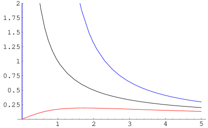
Figure 1: The potential $U$ as function of the auxiliary dilaton $\gamma$.

For evaluation of entropy the auxiliary dilaton $\Phi$ is the relevant field because it multiplies the curvature scalar in the action and therefore the (Gibbons–Hawking) boundary term contains $\Phi$ evaluated at the boundary [26]. Then one may trivially integrate out the abelian $BF$ term as it decouples from all other fields.

Recollection of relevant quantities

The (target space) action (16) is needed in order to be able to discuss entropy of the ESBH. The conformally invariant combination of the dilaton potentials defined in (4) reads

$$w=-b\left(1+\sqrt{1+\gamma^{2}}\right)\,,$$ (22)

where $\gamma$ is an auxiliary field which fulfils (see Eq. (19))

$$\frac{\operatorname{d}\!\gamma}{\operatorname{d}\!\Phi}=1+\frac{1}{\sqrt{1+\gamma^{2}}}\,.$$ (23)

The ADM mass is given by

$$M_{\rm ADM}=\frac{b}{2\pi G}\,k=\frac{2b}{2\pi G}\,M\,,$$ (24)

where $k$ is the level, $b$ an irrelevant scale parameter and the dimensionless quantity $M$ used henceforth lies in the interval $(1,\infty)$. Hawking temperature reads

$$T=\frac{b}{2\pi}\,\sqrt{1-\frac{1}{M}}\,.$$ (25)

The microcanonical entropy in equilibrium takes the form

$$S=\frac{2}{G}\left(\sqrt{M(M-1)}+{\rm arctanh}\,{\sqrt{1-\frac{1}{M}}}\right).$$ (26)

Finally, the specific heat will be needed:

$$C_{V}=\frac{8\pi}{bG}\,M^{2}\,T>0\,.$$ (27)

3.2 Thermal fluctuations vs. α^′ corrections

Application of (8) is possible only if $M\gg 1$. Thus, in order to study thermal fluctuations it is sufficient to expand (26) around $M=\infty$. Therefore, already the equilibrium entropy acquires logarithmic corrections which are $\alpha^{\prime}$ corrections:

$$S=\frac{2}{G}\left(M+\frac{1}{2}\ln{M}+\dots\right).$$ (28)

The leading order term will be denoted by $S^{\mathrm{WBH}}=2M/G=2/((1-(2\pi T/b)^{2})G)$. Note that the subleading term comes with a positive sign. It is emphasized that neither thermal nor quantum fluctuations have been considered so far. If the latter are negligible, i.e., $M\gg 1$, and additionally $\ln{M}\gg|\ln{G}|$ then Eq. (8) together with (28) establishes our main result,

$$S^{\mathrm{ESBH}}_{\mathrm{c}}=S^{\mathrm{WBH}}+\left(1+\frac{1}{G}\right)\ln S^{\mathrm{WBH}}\,.$$ (29)

It should be noted that for corresponding corrections to the microcanonical entropy, as mentioned below (1), the term arising from thermal fluctuations reverses its sign, i.e.,

$$S^{\mathrm{ESBH}}_{\rm mc}=S^{\mathrm{WBH}}-\left(1-\frac{1}{G}\right)\ln{S^{\mathrm{WBH}}}\,.$$ (30)

3.3 Discussion

While for the canonical entropy both corrections increase the entropy, for the microcanonical entropy the following happens: If $G$ is small [large] the $\alpha^{\prime}$ corrections [thermal fluctuations] dominate and yield a positive [negative] prefactor in front of the logarithmic term. If $G=1$ both kind of corrections cancel each other and the “improved” microcanonical entropy of the exact string BH is equal to $S_{\mathrm{WBH}}$, i.e., proportional to the mass. It is stressed that this is a consistent cancellation of logarithmic contributions in the sense that it is not resulting from thermal fluctuations on top of quantum fluctuations, but rather from thermal fluctuations on top of $\alpha^{\prime}$ corrections. However, as already mentioned the use of the microcanonical entropy is difficult to interpret physically if mass is allowed to fluctuate. In any case, the appearance of the dimensionless coupling constant $G$ in (29) due to $\alpha^{\prime}$ corrections seems to be a remarkable new feature in the context of log-corrections to BH entropy.

If $E-TS\neq 0$ there are two possibilities: either work terms are present or energy contains a “Casimir contribution” violating the Euler relation $E=TS$ [40], i.e., a non-extensive component which in $D$ dimensions scales as $E_{C}(S/G)=E_{C}(S)/G^{1-2/D}$, as opposed to the extensive part $E(S/G)=E(S)/G$. In 2D $E_{C}$ does not scale at all (or at most logarithmically). If one defines $E=M_{\mathrm{ADM}}-b/(\pi G)$ one obtains in the absence of fluctuations

$$E-TS=-\frac{b}{\pi G}\sqrt{1-\frac{1}{M}}\,{\rm arctanh}\,{\sqrt{1-\frac{1}{M}}}\approx-\frac{T}{G}\ln{S^{\mathrm{WBH}}}\,.$$ (31)

Because the right hand side above scales extensively with $1/G$ it seems adequate to infer the presence of work terms. They vanish for $E\to 0$. It could be quite interesting to unravel their physical meaning. We will provide but the first step: To this end it is helpful to observe that the right hand side in (31) is nothing but (minus) temperature times the $\alpha^{\prime}$ correction to the (micro-)canonical entropy. Thus, the $\alpha^{\prime}$ corrections are responsible for the violation of $E=TS$.

Finally, it is recalled that the result (8) may be applied to any 2D dilaton gravity model and therefore could be useful for future studies.

I am grateful to D. Vassilevich for discussion and to S. Moskaliuk for important administrative help. Some of the results have been presented at a conference in Prague “Path Integrals. From Quantum Information to Cosmology” in June 2005. The relevant references concerning my talk “Path integral quantization of the ESBH” are contained in appendix B.

Appendix A Basic thermodynamical notions

Entropy may be defined as the maximum of the mean expected information under given constraints, times an irrelevant dimensionful factor, the Boltzmann constant, which will be set to unity in the present work. Although not always a detailed microscopic understanding is available for a given system, especially in BH physics, it is nevertheless useful to adopt the information theoretic approach: For a given discrete ensemble with probability distribution $w_{\nu}$ (where $\sum_{\nu}w_{\nu}=1$, the sum extending over all possible configurations $\nu=1,\dots,N$ and $w_{\nu}\in[0,1]$ being the probability to measure a particular configuration $\nu$) the information for any event $v$ is defined as $-\ln{w_{\nu}}$. Its mean value is $-\sum_{\nu}w_{\nu}\ln{w_{\nu}}$. The canonical entropy in the context of BH physics rests upon the physical constraint $\sum_{\nu}w_{\nu}M_{\nu}=:\left<M\right>=M$:

$$S_{\rm c}=\max\left[-\sum_{\nu}w_{\nu}\ln{w_{\nu}}-\alpha\biggl{(}\sum_{\nu}w_{\nu}-1\biggr{)}-\beta\biggl{(}\sum_{\nu}w_{\nu}M_{\nu}-M\biggr{)}\right].$$ (32)

The quantity $\exp{(1+\alpha)}$ is called partition function and usually is denoted by $Z$. The quantity $T=1/\beta$ is called (Hawking) temperature of the BH. Ensuingly, $S_{\mathrm{c}}=\ln{Z}+M/T$. From $\delta w_{\nu}(\ln{w_{\nu}}+1+\alpha+\beta M_{\nu})=0$ one deduces $w_{\nu}=\exp{(-M_{\nu}/T)}/Z$. The first law of thermodynamics/BH mechanics,

$$\operatorname{d}\!M=T\operatorname{d}\!S_{\rm c}\,,$$ (33)

is a simple consequence. Work terms are assumed to be absent, which is sufficient for our purposes.

The microcanonical entropy, $S_{\rm mc}$, may be obtained as a special case from the canonical entropy where only states with the same value of $M_{\nu^{\prime}}$ are considered, $S_{\mathrm{mc}}=\ln\rho$, where $\rho=1/w_{\nu^{\prime}}=Z\exp{(M_{\nu^{\prime}}/T)}$ is the corresponding number of microstates (which necessarily are equally distributed). Apart from rare but interesting exceptions the equilibrium values of canonical and microcanonical entropies coincide. Such an exception arises, for instance, if the microcanonical specific heat,

$$C_{\rm mc}=-\frac{\left(S^{\prime}_{\rm mc}\right)^{2}}{S^{\prime\prime}_{\rm mc}}\,,$$ (34)

is negative, where prime denotes differentiation with respect to $M$.

In the continuum case sums are replaced by integrals and $\rho(M)$ becomes the density of states at a given mass $M$. The partition function may be considered as the Laplace transformed density of states,

$$Z(\beta)=\int_{0}^{\infty}\rho(M)\E^{-\beta M}\operatorname{d}\!M=\int_{0}^{\infty}\E^{S_{\rm mc}(M)-\beta M}\operatorname{d}\!M\,.$$ (35)

This formula allows to derive corrections to the partition function from thermal fluctuations in the mass.

If there are two subsystems which may exchange energy (like a BH and radiation) then the total entropy $S_{\rm tot}$ is the maximum of the sum of the entropies $S_{1}$, $S_{2}$ of the subsystems under the constraint that $E_{1}+E_{2}=E$, where $E$ is a constant, the total energy, and $E_{1}$, $E_{2}$ are the energies of the subsystems. Variation under such a constraint yields that the temperatures of both subsystems have to be equal. However, equality of temperatures only establishes an extremum of the total entropy. For a maximum in addition the inequality

$$\frac{\partial^{2}S_{1}}{\partial E_{1}^{2}}+\frac{\partial^{2}S_{2}}{\partial E_{2}^{2}}<0\,,$$ (36)

has to be fulfilled. Defining the (canonical) specific heat as

$$C_{V}:=-\beta^{2}\,\frac{\partial^{2}\ln{Z}}{\partial\beta^{2}}=T\,\frac{\partial S_{\rm c}}{\partial T}\,,$$ (37)

one can see that (36) holds if the specific heat of each subsystem, in particular of the BH, is positive.

Appendix B Path integral quantization of the ESBH

This appendix is much closer to the actual content of my talk at the conference “Path Integrals: From Quantum Information to Cosmology” in Prague, but as it does not contain essential new considerations I shall be very brief and provide mainly a pointer to the literature. For a first orientation and a more comprehensive list of references the review article Ref. [18] may be consulted. Below the emphasis will be on the “Vienna School approach”. The basic feature discriminating it from other approaches, like Dirac quantization (cf. e.g. [42]), is the possibility to integrate out geometry exactly even in the presence of matter, thus obtaining an effective theory with nonlocal and nonpolynomial matter interactions. The latter is a suitable starting point for a perturbative treatment where to each given order geometry may be reconstructed self-consistently. The path integral formulation appears to be the most adequate language to derive these perturbative results.

Various aspects of the path integral quantization of generic dilaton gravity (including different signatures and supergravity extensions) with matter have been discussed in a series of publications [43] which, in a sense, are built upon the two basic papers of Kummer and Schwarz [44]. In particular, $S$-matrix calculations where “Virtual Black Holes” emerge as intermediate states have been performed and discussed in Refs. [45, 46, 47, 48]. Previous proceedings contributions may also be of use as a further literature guide [49]. It is emphasized that the first order formulation mentioned in footnote 4 has been a crucial technical ingredient.

Applying this formalism to the ESBH is possible since a suitable target space action has been constructed [4]. If the geometric action (3) is supplemented by scalar matter (e.g. the tachyon)

$$L^{(m)}=\int_{\mathcal{M}_{2}}\operatorname{d}\!^{2}x\sqrt{-g}\Bigl{(}F(\Phi)(\nabla\phi)^{2}+f(\Phi,\phi)\Bigr{)}\,,$$ (38)

where $F$ is the coupling function and $\phi$ the scalar field, exact solutions emerge only for very specific cases as the system now exhibits one propagating physical degree of freedom. The considerations of local self interactions encoded in the function $f$ is straightforward and for simplicity will be omitted here. Since the conference has been on Path Integrals it is appropriate to provide the latter at least schematically

$$\begin{array}[]{rcl}W(\mathrm{sources})&=&\disty\int\mathcal{D}(\mathrm{geometry})\,\mathcal{D}(\mathrm{dilaton})\,\mathcal{D}(\mathrm{ghosts})\,\mathcal{D}\phi\times\\[9.0pt] &&\disty\times\exp\left[\I\int\operatorname{d}\!^{2}x\left(\mathcal{L}^{\mathrm{eff}}(\mathrm{geometry},\mathrm{dilaton},\mathrm{ghosts},\phi)+\mathrm{sources}\right)\right].\end{array}$$ (39)

Path integration over all fields but matter is possible exactly, without introducing a fixed background geometry. Thus, the quantization procedure is non-perturbative and background independent. However, there are ambiguities coming from integration constants the fixing of which selects a certain asymptotics of spacetime; two of them are trivial while the third one essentially determines the ADM mass (whenever this notion makes sense). Thus, background independence holds only in the bulk but fails to hold in the asymptotic region; we regard this actually as an advantage for describing scattering processes because there is no “background independent asymptotic observer”. What one ends up with is a generating functional for Green functions depending solely on the matter field $\phi$, the corresponding source $\sigma$ and on the integration constants mentioned in the previous paragraph [47]:

$$W(\sigma) = \int(\mathcal{D}\phi)\exp\Bigl{[}\I\int\operatorname{d}\!^{2}x(\mathcal{L}^{\rm eff}+\sigma\phi)\Bigr{]}\,,$$

$$\mathcal{L}^{\rm eff} = F(\hat{\Phi})\partial_{0}\phi\partial_{1}\phi-\tilde{g}w^{\prime}(\hat{\Phi})\,.$$ (40)

The constant $\tilde{g}$ is an effective coupling which turns out to be inessential and may be absorbed by a redefinition of the unit of length. For minimal coupling ($F=\rm const.$) $w^{\prime}$ is the only source for matter vertices. It is a non-polynomial function, in general. Moreover, the quantity $\hat{\Phi}$, which is the quantum version of the dilaton $\Phi$, depends not only on integration constants but also non-locally on matter; to be more precise, it depends non-locally on $(\partial_{0}\phi)^{2}$ due to the appearance of the operator $\partial_{0}^{-1}$. Thus, in general the effective Lagrangian density (40) is non-local and non-polynomial in the matter field.

Figure 2: The total $V^{(4)}$-vertex (with outer legs).

The classical vertices are generated by the conformally invariant combination of potentials defined in (4). Evidently, constant and linear contributions to the function $w$ are of no relevance for vertices. Perturbation theory yields to lowest order the two Feynman diagrams depicted in figure 2. The total $V^{(4)}$-vertex (with outer legs) contains a symmetric contribution $V^{(4)}_{a}$ and (for non-minimal coupling) a non-symmetric one $V^{(4)}_{b}$. The shaded blobs depict the intermediate interactions with virtual BHs. With the abbreviations

$$\phi_{0}:=\sfrac 12\,(\partial_{0}\phi)^{2}\,,\qquad\phi_{1}:=\sfrac 12\,(\partial_{0}\phi)(\partial_{1}\phi)\,,$$

the Feynman rules for the lowest order non-local vertices read [47]:

$$V_{a}^{(4)}=-2\int_{x}\int_{y}\phi_{0}(x)\phi_{0}(y)\theta(x^{0}-y^{0})\delta(x^{1}-y^{1})F(x^{0})F(y^{0})\times\hskip 56.9055pt$$

$$\times\Bigg{[}4\left(w(x^{0})-w(y^{0})\right)-2(x^{0}-y^{0})\Big{(}w^{\prime}(x^{0})+w^{\prime}(y^{0})+$$

$$\qquad+\frac{F^{\prime}(x^{0})}{F(x^{0})}\left(w(x^{0})+M_{\mathrm{ADM}}\right)+\frac{F^{\prime}(y^{0})}{F(y^{0})}\left(w(y^{0})+M_{\mathrm{ADM}}\right)\Big{)}\Bigg{]}\,,$$ (41)

and

$$V_{b}^{(4)}=-4\int_{x}\int_{y}\phi_{0}(x)\phi_{1}(y)\delta(x^{1}-y^{1})F(x^{0})F^{\prime}(y^{0})\left|x^{0}-y^{0}\right|\,.$$ (42)

For the simpler case of minimal coupling, $F=\rm const.$, the non-symmetric vertex $V_{b}^{(4)}$ vanishes and the symmetric one for the ESBH simplifies to

$$\begin{array}[]{rcl}V^{(a)}_{\mathrm{ESBH}}&=&\disty-2F^{2}\int_{x}\int_{y}\phi_{0}(x)\phi_{0}(y)\theta(x^{0}-y^{0})\delta(x^{1}-y^{1})\times\\[9.0pt] &&\disty\times\left[4\bigl{(}w(x^{0})-w(y^{0})\bigr{)}-2(x^{0}-y^{0})\biggl{(}\frac{w(x^{0})\gamma(x^{0})}{\gamma^{2}(x^{0})+1}+\frac{w(y^{0})\gamma(y^{0})}{\gamma^{2}(y^{0})+1}\biggr{)}\right],\end{array}$$ (43)

with $w$ as defined in Eqs. (22) and (23).

The $S$-matrix element with ingoing modes $q$, $q^{\prime}$ and outgoing ones $k$, $k^{\prime}$,

$$T(q,q^{\prime};k,k)=\frac{1}{2}\left<0\left|a^{-}_{k}a^{-}_{k^{\prime}}\left(V^{(4)}_{a}+V^{(4)}_{b}\right)a^{+}_{q}a^{+}_{q^{\prime}}\right|0\right>,$$ (44)

depends not exclusively on the vertices (41), (42), but also on the asymptotic states of the scalar field with corresponding creation/anihilation operators $a^{\pm}$ obeying canonical commutation relations of the form $\left[a^{-}_{k},a^{+}_{k^{\prime}}\right]\propto\delta(k-k^{\prime})$. Asymptotically the Klein–Gordon equation with $K:=M_{\mathrm{ADM}}+w(x^{0})$ reads

$$\partial_{0}\left(\partial_{1}+K\partial_{0}\right)\phi=-\frac{F^{\prime}(x^{0})}{2F(x^{0})}\,\left(\partial_{1}+2K\partial_{0}\right)\phi\,,$$ (45)

If (45) can be solved exactly and the set of solutions is complete and normalizable (in an appropriate sense) a Fock space for incoming and outgoing scalars can be constructed in the usual way. Since the integration constant $M_{\mathrm{ADM}}$ enters (45) the asymptotic states depend on the choice of boundary conditions. Physically, the scalar particles are scattered on their own gravitational self-energy (the “Coulomb gravitons” have been integrated out).

It appears to be straightforward to solve (45) for minimal coupling and to calculate the $S$-matrix (44) with (43). Such a calculation is of interest (but will not be performed here) because for the Witten BH [27, 11], which arises as limit of the ESBH, the function $w$ is linear and therefore exhibits scattering triviality [47]. Obviously, the $\alpha^{\prime}$ corrections implicit in the ESBH are able to transcend this triviality result.

References

- [1] D.N. Page: hep-th/0409024.
-
[2]
V.P. Frolov and D.V. Fursaev,
Class. Quant. Grav. 15 (1998) 2041,
hep-th/9802010;
R. M. Wald, Living Rev. Rel. 4 (2001) 6, gr-qc/9912119;
T. Padmanabhan, Phys. Rept. 406 (2005) 49, gr-qc/0311036;
T. Damour, hep-th/0401160;
S. Das, Pramana 63 (2004) 797 hep-th/0403202;
D.V. Fursaev, Phys. Part. Nucl. 36 (2005) 81, [Fiz. Elem. Chast. Atom. Yadra 36 (2005) 146], gr-qc/0404038. - [3] R. Dijkgraaf, H. Verlinde and E. Verlinde: Nucl. Phys. B 371 (1992) 269.
- [4] D. Grumiller: JHEP 05 (2005) 028, hep-th/0501208.
-
[5]
V.P. Frolov, W. Israel and S.N. Solodukhin: Phys. Rev. D
54 (1996) 2732, hep-th/9602105;
S.N. Solodukhin: Phys. Rev. D 57 (1998) 2410, hep-th/9701106;
R.B. Mann and S.N. Solodukhin: Nucl. Phys. B 523 (1998) 293, hep-th/9709064;
A.J.M. Medved and G. Kunstatter: Phys. Rev. D 60 (1999) 104029, hep-th/9904070. -
[6]
R.K. Kaul and P. Majumdar: Phys. Rev. Lett. 84 (2000)
5255, gr-qc/0002040;
S. Carlip: Class. Quant. Grav. 17 (2000) 4175, gr-qc/0005017;
J.-l. Jing and M.-L. Yan: Phys. Rev. D 63 (2001) 024003, gr-qc/0005105;
D. Birmingham and S. Sen: Phys. Rev. D 63 (2001) 047501, hep-th/0008051;
D. Birmingham, I. Sachs and S. Sen: Int. J. Mod. Phys. D 10 (2001) 833, hep-th/0102155;
D. Birmingham, K.S. Gupta and S. Sen: Phys. Lett. B 505 (2001) 191, hep-th/0102051;
K.S. Gupta and S. Sen: Phys. Lett. B 526 (2002) 121, hep-th/0112041;
J.E. Lidsey, S. Nojiri, S.D. Odintsov and S. Ogushi: Phys. Lett. B 544 (2002) 337, hep-th/0207009. - [7] S. Das, P. Majumdar and R.K. Bhaduri: Class. Quant. Grav. 19 (2002) 2355, hep-th/0111001.
-
[8]
M.R. Setare: Eur. Phys. J. C 33 (2004) 555,
hep-th/0309134;
A. Chatterjee and P. Majumdar: Phys. Rev. Lett. 92 (2004) 141301, gr-qc/0309026;
M.-I. Park: JHEP 12 (2004) 041, hep-th/0402173. - [9] L.D. Landau and E.M. Lifshitz: Statistical Physics, ch. XII. Pergamon, 1969.
- [10] J. Preskill, P. Schwarz, A.D. Shapere, S. Trivedi and F. Wilczek: Mod. Phys. Lett. A 6 (1991) 2353.
- [11] C.G. Callan, Jr., S.B. Giddings, J.A. Harvey and A. Strominger: Phys. Rev. D 45 (1992) 1005, hep-th/9111056.
-
[12]
J.G. Russo, L. Susskind and L. Thorlacius: Phys. Lett. B
292 (1992) 13, hep-th/9201074; Phys. Rev. D
46 (1992) 3444, hep-th/9206070; Phys. Rev. D
47 (1993) 533, hep-th/9209012;
S.P. de Alwis: Phys. Lett. B 289 (1992) 278, hep-th/9205069; Phys. Lett. B 300 (1993) 330, hep-th/9206020;
A. Bilal and C.G. Callan: Nucl. Phys. B 394 (1993) 73, hep-th/9205089;
S. Bose, L. Parker and Y. Peleg: Phys. Rev. D 52 (1995) 3512, hep-th/9502098;
S.N. Solodukhin: Phys. Rev. D 53 (1996) 824, hep-th/9506206. - [13] A. Achucarro and M.E. Ortiz: Phys. Rev. D 48 (1993) 3600, hep-th/9304068.
-
[14]
M. Banados, C. Teitelboim and J. Zanelli: Phys. Rev. Lett.
69 (1992) 1849, hep-th/9204099;
M. Banados, M. Henneaux, C. Teitelboim and J. Zanelli: Phys. Rev. D 48 (1993) 1506, gr-qc/9302012. -
[15]
G. Guralnik, A. Iorio, R. Jackiw and S.Y. Pi: Ann. Phys.
308 (2003) 222, hep-th/0305117;
D. Grumiller and W. Kummer: Ann. Phys. 308 (2003) 211, hep-th/0306036;
L. Bergamin, D. Grumiller, A. Iorio and C. Nuñez: JHEP 11 (2004) 021, hep-th/0409273. -
[16]
T. Takayanagi and N. Toumbas: JHEP 07 (2003) 064,
hep-th/0307083;
M.R. Douglas et al.: hep-th/0307195;
D.M. Thompson: Phys. Rev. D 70 (2004) 106001, hep-th/0312156;
A. Strominger: JHEP 03 (2004) 066, hep-th/0312194;
S. Gukov, T. Takayanagi and N. Toumbas: JHEP 03 (2004) 017, hep-th/0312208;
J.L. Davis, L.A. Pando Zayas and D. Vaman: JHEP 03 (2004) 007, hep-th/0402152;
U.H. Danielsson, J.P. Gregory, M.E. Olsson, P. Rajan and M. Vonk: JHEP 04 (2004) 065, hep-th/0402192. - [17] J.L. Davis and R. McNees: hep-th/0411121.
- [18] D. Grumiller, W. Kummer and D.V. Vassilevich: Phys. Rept. 369 (2002) 327, hep-th/0204253.
- [19] P. Schaller and T. Strobl: Mod. Phys. Lett. A 9 (1994) 3129, hep-th/9405110.
- [20] T. Klösch and T. Strobl: Class. Quant. Grav. 13 (1996) 965, gr-qc/9508020; Class. Quant. Grav. 13 (1996) 2395, gr-qc/9511081; Class. Quant. Grav. 14 (1997) 1689, hep-th/9607226.
-
[21]
J.G. Russo and A.A. Tseytlin: Nucl. Phys. B 382 (1992)
259, hep-th/9201021;
S.D. Odintsov and I.L. Shapiro: Phys. Lett. 263 (1991) 183. -
[22]
R.M. Wald: Phys. Rev. D 48 (1993) 3427,
gr-qc/9307038;
V. Iyer and R. M. Wald, Phys. Rev. D 50 (1994) 846, gr-qc/9403028. - [23] J. Gegenberg, G. Kunstatter and D. Louis-Martinez: Phys. Rev. D 51 (1995) 1781, gr-qc/9408015.
- [24] G. Lopes Cardoso, B. de Wit and T. Mohaupt: Phys. Lett. B 451 (1999) 309, hep-th/9812082.
-
[25]
A. Strominger: JHEP 01 (1999) 007,
hep-th/9809027;
M. Cadoni and S. Mignemi: Phys. Rev. D 59 (1999) 081501, hep-th/9810251;
S. Carlip: Phys. Rev. Lett. 82 (1999) 2828, hep-th/9812013;
S.N. Solodukhin: Phys. Lett. B 454 (1999) 213, hep-th/9812056;
M.-I. Park and J. Ho: Phys. Rev. Lett. 83 (1999) 5595, hep-th/9910158;
S. Carlip: Phys. Rev. Lett. 83 (1999) 5596, hep-th/9910247;
M.-I. Park and J.H. Yee: Phys. Rev. D 61 (2000) 088501, hep-th/9910213;
G. Kang, J.-i. Koga and M.-I. Park: Phys. Rev. D 70 (2004) 024005, hep-th/0402113;
S. Carlip: hep-th/0408123;
V.O. Soloviev,: gr-qc/0507124. - [26] L. Bergamin, D. Grumiller, W. Kummer and D. Vassilevich: in preparation.
-
[27]
G. Mandal, A.M. Sengupta and S.R. Wadia: Mod. Phys. Lett. A
6 (1991) 1685;
S. Elitzur, A. Forge and E. Rabinovici: Nucl. Phys. B 359 (1991) 581;
E. Witten: Phys. Rev. D 44 (1991) 314. -
[28]
C. Teitelboim: Phys. Lett. B 126 (1983) 41;
R. Jackiw: Nucl. Phys. B 252 (1985) 343. -
[29]
T.M. Fiola, J. Preskill, A. Strominger and S.P. Trivedi: Phys.
Rev. D 50 (1994) 3987, hep-th/9403137;
R.C. Myers: Phys. Rev. D 50 (1994) 6412, hep-th/9405162;
J.D. Hayward: Phys. Rev. D 52 (1995) 2239, gr-qc/9412065;
O.B. Zaslavsky: Phys. Lett. B 375 (1996) 43. - [30] A.A. Tseytlin: Phys. Lett. B 268 (1991) 175.
- [31] I. Jack, D.R.T. Jones and J. Panvel: Nucl. Phys. B 393 (1993) 95, hep-th/9201039.
- [32] A.A. Tseytlin: Nucl. Phys. B 399 (1993) 601, hep-th/9301015.
- [33] I. Bars and K. Sfetsos: Phys. Rev. D 48 (1993) 844, hep-th/9301047.
- [34] K. Becker: hep-th/9404157.
- [35] V.A. Kazakov and A.A. Tseytlin: JHEP 06 (2001) 021, hep-th/0104138.
- [36] M.J. Perry and E. Teo: Phys. Rev. Lett. 70 (1993) 2669, hep-th/9302037.
- [37] P. Yi: Phys. Rev. D 48 (1993) 2777, hep-th/9302070.
- [38] G.W. Gibbons and M.J. Perry: Int. J. Mod. Phys. D 1 (1992) 335, hep-th/9204090.
- [39] D. Grumiller and D.V. Vassilevich: JHEP 11 (2002) 018, hep-th/0210060.
- [40] E. Verlinde: hep-th/0008140.
- [41] H. Touchette: Equivalence and Nonequivalence of Microcanonical and Canonical Ensembles: A Large Deviations Study. PhD thesis, McGill University, Montreal, 2003.
-
[42]
D. Cangemi and R. Jackiw: Phys. Rev. Lett. 69 (1992) 233,
hep-th/9203056;
A. Mikovic: Phys. Lett. B 291 (1992) 19, hep-th/9207006;
D. Cangemi and R. Jackiw: Phys. Lett. B 299 (1993) 24, hep-th/9210036;
A. Mikovic: Phys. Lett. B 304 (1993) 70, hep-th/9211082;
J. Gegenberg and G. Kunstatter: Phys. Rev. D 47 (1993) 4192, gr-qc/9302006;
D. Cangemi and R. Jackiw: Ann. Phys. 225 (1993) 229, hep-th/9302026;
D. Louis-Martinez, J. Gegenberg and G. Kunstatter: Phys. Lett. B 321 (1994) 193, gr-qc/9309018;
K.V. Kuchař: Phys. Rev. D 50 (1994) 3961, gr-qc/9403003;
T. Strobl: Phys. Rev. D 50 (1994) 7346, hep-th/9403121;
D. Cangemi and R. Jackiw: Phys. Lett. B 337 (1994) 271, hep-th/9405119;
A. Mikovic: Phys. Lett. B 355 (1995) 85, hep-th/9407104;
M. Cavaglia, V. de Alfaro and A.T. Filippov: Int. J. Mod. Phys. D 4 (1995) 661, gr-qc/9411070;
D. Cangemi, R. Jackiw and B. Zwiebach: Ann. Phys. 245 (1996) 408, hep-th/9505161;
M. Varadarajan: Phys. Rev. D 52 (1995) 7080, gr-qc/9508039;
A. Barvinsky and G. Kunstatter: Phys. Lett. B 389 (1996) 231, hep-th/9606134;
K.V. Kuchař, J.D. Romano and M. Varadarajan: Phys. Rev. D 55 (1997) 795, gr-qc/9608011;
J. Gegenberg, G. Kunstatter and T. Strobl: Phys. Rev. D 55 (1997) 7651, gr-qc/9612033;
M. Cavaglia, V. de Alfaro and A.T. Filippov: Phys. Lett. B 424 (1998) 265, hep-th/9802158. -
[43]
F. Haider and W. Kummer: Int. J. Mod. Phys. A 9 (1994)
207;
W. Kummer, H. Liebl and D.V. Vassilevich: Nucl. Phys. B 493 (1997) 491, gr-qc/9612012;
Nucl. Phys. B 544 (1999) 403, hep-th/9809168;
L. Bergamin, D. Grumiller, W. Kummer and D.V. Vassilevich: Class. Quant. Grav. 22 (2005) 1361, hep-th/0412007;
L. Bergamin, D. Grumiller and W. Kummer: JHEP 05 (2004) 060, hep-th/0404004;
L. Bergamin: hep-th/0408229. - [44] W. Kummer and D.J. Schwarz: Phys. Rev. D 45 (1992) 3628; Nucl. Phys. B 382 (1992) 171.
-
[45]
D. Grumiller, W. Kummer and D.V. Vassilevich: Nucl. Phys. B
580 (2000) 438, gr-qc/0001038;
P. Fischer, D. Grumiller, W. Kummer and D.V. Vassilevich: Phys. Lett. B 521 (2001) 357, gr-qc/0105034. Erratum ibid. 532 (2002) 373;
D. Grumiller: Class. Quant. Grav. 19 (2002) 997, gr-qc/0111097;
D. Grumiller, W. Kummer and D.V. Vassilevich: JHEP 07 (2003) 009, hep-th/0305036. - [46] D. Grumiller: Quantum dilaton gravity in two dimensions with matter. PhD thesis, Technische Universität Wien, 2001; gr-qc/0105078.
- [47] D. Grumiller, W. Kummer and D.V. Vassilevich: European Phys. J. C 30 (2003) 135, hep-th/0208052.
- [48] D. Grumiller: Int. J. Mod. Phys. D 13 (2004) 1973, hep-th/0409231.
-
[49]
D. Grumiller: Int. J. Mod. Phys. A 17 (2001) 989,
hep-th/0111138;
in Proceedings of International Workshop on Mathematical
Theories and their Applications, S. Moskaliuk, ed., pp. 59–96,
TIMPANI. Cernivtsi, Ukraine, 2004. hep-th/0305073;
gr-qc/0311011; Invited talk at MG X;
D. Grumiller and W. Kummer: in What comes beyond the Standard Model? Symmetries beyond the standard model, N.M. Borstnik, H.B. Nielsen, C.D. Froggatt, and D. Lukman, eds., vol. 4 of Bled Workshops in Physics, pp. 184–196, EURESCO. Portoroz, Slovenia, July, 2003. gr-qc/0310068, based upon two talks. - [50] H. Liebl, D.V. Vassilevich and S. Alexandrov: Class. Quant. Grav. 14 (1997) 889, gr-qc/9605044.
-
[51]
T. Banks and M. O’Loughlin: Nucl. Phys. B 362 (1991)
649;
V.P. Frolov: Phys. Rev. D 46 (1992) 5383;
R.B. Mann: Phys. Rev. D 47 (1993) 4438, hep-th/9206044. - [52] H. Grosse, W. Kummer, P. Presnajder and D.J. Schwarz: J. Math. Phys. 33 (1992) 3892, hep-th/9205071.
- [53] D. Grumiller and D. Mayerhofer: Class. Quant. Grav. 21 (2004) 5893, gr-qc/0404013.
- [54] D. Grumiller and W. Kummer: Phys. Rev. D 61 (2000) 064006, gr-qc/9902074.