Braneworld Flux Inflation

Abstract

We propose a geometrical model of brane inflation where inflation is driven by the flux generated by opposing brane charges and terminated by the collision of the branes, with charge annihilation. We assume the collision process is completely inelastic and the kinetic energy is transformed into the thermal energy after collision. Thereafter the two branes coalesce together and behave as a single brane universe with zero effective cosmological constant. In the Einstein frame, the 4-dimensional effective theory changes abruptly at the collision point. Therefore, our inflationary model is necessarily 5-dimensional in nature. As the collision process has no singularity in 5-dimensional gravity, we can follow the evolution of fluctuations during the whole history of the universe. It turns out that the radion field fluctuations have a steeply tilted, red spectrum, while the primordial gravitational waves have a flat spectrum. Instead, primordial density perturbations could be generated by a curvaton mechanism.

I Introduction

Recent cosmological observations such as the WMAP results are consistent with the inflationary scenario. Hence, we are prompted to seek the inflaton in a unified theory of particle physics. Currently, it is widely believed that the most promising candidate for a unified theory is superstring theory. Interestingly, the superstring theory predicts the existence of the extra dimensions. In order to reconcile this prediction with our observed 4-dimensional universe, we need a mechanism to hide the extra dimensions. For a long time, the Kaluza-Klein compactification was considered to be the unique choice. However, recent developments in superstring theory suggest a braneworld picture where we are living on 4-dimensional hypersurface embedded in a higher dimensional spacetime Horava . This braneworld picture not only gives a way for the superstring theory to be phenomenologically viable but also suggests a new inflationary scenario, so-called brane inflation Dvali ; Kachru .

In the brane inflation scenario, the radion, the distance between branes, plays the role of the inflaton and inflation is terminated by the brane collision. This is nice because the inflation is realized purely geometrical manner without introducing an ad-hoc scalar field. In this scenario, however, branes are treated as test branes. On the other hand, relativistic cosmologists have studied the braneworld gravity intensively review . In these studies, the effect of the bulk geometry on the 4-dimensional braneworld cosmology have been a central concern, though inflation is usually assumed to be driven by the fundamental scalar field either on the brane or in the bulk. In this braneworld cosmology, the self-gravity of branes are properly treated and hence, it is clear how to calculate corrections due to the bulk effect MWBH ; LMWgw ; KKS ; HS . Taking a look at both approaches, we have come up with the idea of incorporating geometrical inflation in a simple Randall-Sundrum (RS) model RS1 .

In this paper, we would like to propose an inflationary scenario driven by the flux generated by a brane that is charged with respect to a five-form field strength. The idea is very similar to that of brane inflation but we take into account the self-gravity of branes. Our model is constructed in the RS framework RS1 . We suppose that initially two positive tension branes are inflating as de Sitter spacetimes embedded in an anti-de Sitter bulk. Eventually, they collide with each other and inflation will end. Subsequently, two branes are assumed to coallesce and evolve as a single $Z_{2}$-symmetric positive tension brane. The gravitational theory is non-singular and the model we construct is essentially 5-dimensional way. Except at the collision point, we can use the effective action obtained by the low energy approximation KS1 ; KS2 ; wiseman . But in the 4-dimensional Einstein frame, the evolution of the universe is discontinuous at the collision point, which means that the effective 4-dimensional theory breaks down. However at the collision point we can use 5-dimensional energy-momentum conservation to determine the dynamics LMW . We are thus able to analyze the spectrum of primordial scalar and tensor fluctuations produced after the collision. It turns out that a curvaton-type mechanism is required to generate the primordial density perturbations producing the present structure of the universe.

The organization of this paper is as follows. In sec.II, the basic setup is presented. In sec.III, our cosmological scenario is described. Inflation driven by the flux is analyzed both in the induced metric frame and the Einstein frame. The consistency analysis gives the expansion rate after the collision determined by the expansion rate of both branes before the collision. The cosmological history after the collision is briefly summarized. In sec.IV, the spectrum of fluctuations are calculated. The sec.V is devoted to conclusions. In the appendix, the detailed derivation of the effective action is provided.

II Basic Setup

The point of brane inflation is that no fundamental scalar field is necessary and the exit from inflation is realized by the collision of branes. What we want to do is to incorporate this idea into the codimension-one RS braneworld model.

We consider a two-brane system where one has a $Z_{2}$ symmetry and the other does not. Hereafter, we call the former the boundary brane and the latter the bulk brane. As we show in an appendix such a set-up can be realised as the limiting case of a three-brane system, with two boundary branes, where one of the $Z_{2}$-symmetric branes is sent to infinity.

The model is described by the 5-dimensional action

$$S = \frac{1}{2\kappa^{2}}\int d^{5}x\sqrt{-g}\left[\overset{(5)}{R}+2\Lambda\right]+\sum_{i=1}^{2}\frac{1}{\kappa^{2}}\int d^{4}x\sqrt{-h_{i}}K^{i}$$ (1)

$$-\frac{1}{2\cdot 5!}\int d^{5}x\sqrt{-g}F_{5}^{2}+\sum_{i=1}^{2}\mu_{i}\int C_{4}$$

$$+\frac{1}{4!}\int d^{5}x\partial_{A}\left(\sqrt{-g}F^{ABCDE}C_{BCDE}\right)$$

$$+\sum_{i=1}^{2}\int d^{4}x\sqrt{-h_{i}}\left[-\sigma_{i}+{\cal L}^{i}_{\rm matter}\right]$$

where $\kappa^{2}$ is the 5-dimensional gravitational coupling constant and $\overset{(5)}{R}$ is the 5-dimensional curvature. Both our branes have positive tension, $\sigma_{1},\sigma_{2}>0$, but opposite charges, $\mu_{1}>0,\ \mu_{2}<0$, which couple to a 4-form potential field, $C_{4}=(1/4!)C_{ABCD}dx^{A}\wedge dx^{B}\wedge dx^{C}\wedge dx^{D}$. The bulk brane separates the bulk into regions $I$ and $I\!I$ (see FIG.1).

We denote the induced metric on each brane by $h_{i\mu\nu}$ and $K^{i}$ denotes the trace-part of the extrinsic curvature of each brane. Here we have taken into account the Gibbons-Hawking boundary term instead of introducing delta-function singularities in the five-dimensional curvature. We incorporated the 5-form field $F_{5}=dC_{4}$ which can change the effective cosmological constant in the bulk $\Lambda$ TS . The third line represents the surface term which is introduced to make the variation of the action with fixed $F_{5}$ consistent.

Let us take the coordinate system

$$ds^{2}=dy^{2}+g_{\mu\nu}(y,x)dx^{\mu}dx^{\nu}$$ (2)

The Latin indices $\{A,B,\cdots\}$ and the Greek indices $\{\mu,\nu,\cdots\}$ are used for tensors defined in the bulk and on the brane, respectively. The 5-form equation of motion becomes

$$\partial_{M}\left(\sqrt{-g}F^{0123y}\right)dx^{M}+\sum_{i=1}^{2}\mu_{i}\delta(y-\phi_{i}(x))dy=0$$ (3)

where $\phi_{i}(x)$ denotes the position of each brane. In each bulk ($y\neq\phi_{i}$), it is easy to solve Eq. (3) as

$$F_{I}^{0123y}=\frac{c_{I}}{\sqrt{-g}}\ ,\quad F_{I\!I}^{0123y}=\frac{c_{I\!I}}{\sqrt{-g}}\ .$$ (4)

where $c_{I},c_{II}$ are constants of integration. Because of the charge conservation, we have $c_{I\!I}=0$ as is explained in the appendix. Thus we see $F_{5}$ has no local dynamics. As $F_{5}$ is not dynamical, we can eliminate it from the action by simply substituting the above solution into the original action. This can be done using the equations of motion to give

$$\frac{1}{4!}\int d^{5}x\partial_{A}\left(\sqrt{-g}F^{ABCDE}C_{BCDE}\right)$$

$$=\frac{1}{5!}\int d^{5}xF_{5}^{2}+\int d^{5}x\partial_{y}\left(\sqrt{-g}F^{0123y}\right)C_{0123}$$

$$=-\int_{I}d^{5}xc_{I}^{2}-\sum_{i=1}^{2}\mu_{i}\int d^{4}xC_{0123}\ .$$ (5)

Substituting Eq. (5) into the original action (1), we see that 4-form potentials are cancelled and the effect of 5-form field strength is indistinguishable from a cosmological constant term in the bulk. Thus, the resultant action is

$$S = \frac{1}{2\kappa^{2}}\int_{I}d^{5}x\sqrt{-g}\left[\overset{(5)}{R}+2\Lambda-\kappa^{2}c_{I}^{2}\right]$$ (6)

$$+\frac{1}{2\kappa^{2}}\int_{I\!I}d^{5}x\sqrt{-g}\left[\overset{(5)}{R}+2\Lambda\right]$$

$$+\sum_{i}\frac{1}{\kappa^{2}}\int\sqrt{-h_{i}}K^{i}$$

$$+\sum_{i}\int d^{4}x\sqrt{-h_{i}}\left[-\sigma_{i}+{\cal L}^{i}_{\rm matter}\right]\ .$$

The 5-form field strength $F_{5}$ in region $I$ acts like a change in the effective 5-dimensional cosmological constant in region $I$, $\Lambda_{I}\equiv\Lambda-\kappa^{2}c_{I}^{2}/2$. Consequently, two bulk regions have a different cosmological constant. The absolute value of the cosmological constant in region I is assumed to be small and therefore we shall see that the effective cosmological constants induced on both branes are positive.

If the expansion rate of the second brane is faster than that of first, both branes will eventually collide with each other and the opposing charges annihilate. The resulting brane tension is assumed to become (close to) the Randall-Sundrum tuning value so that the inflation ends and the universe becomes radiation dominated. We assume a completely inelastic collision so that the kinetic energy of the branes is transformed into radiation energy density on the brane. The subsequent evolution is same as that of the radiation dominated universe in the RSII brane model. Thus, the original flux generated by the charged branes has caused de Sitter inflation of branes and the exit from inflation is realized by the brane collision. In the following sections, we shall look at the details of this scenario.

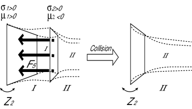
Figure 1: The 3-brane charges produce $F_{5}$ flux in the region I. This changes the cosmological constant in region I. After the collision, the single brane remains and the big-bang universe commences.

III Flux Inflation

The non-linear dynamics of de Sitter branes embedded in 5-dimensional anti-de Sitter space can be studied exactly without recourse to any approximation kaloper ; BCG ; radion . However the study of inhomogeneous perturbations about this background, when two de Sitter branes are in relative motion, is a much harder problem. Therefore we will use a low-energy approximation KS1 ; wiseman ; KS2 ; sugumi in this case, valid when the Hubble rate is smaller than the anti-de Sitter scale. In this case the only extra degree of freedom coming from the 5-dimensional gravitational field is the radion, a scalar in the 4-dimensional effective theory, describing the distance between the two branes.

Before the collision, the radion field is non-minimally coupled to the 4-dimensional gravitational field on either brane and the system is described by the scalar-tensor theory. Hence, it is useful to look at the cosmological evolution both from the induced metric frame on the bulk brane and the Einstein frame. After the collision the radion field vanishes and the low-energy system is described by 4-dimensional Einstein gravity. As the collision changes the theory discontinuously, the evolution of the universe in the Einstein frame looks strange. We find a contracting universe immediately before the collision which will start to expand abruptly after the collision. However, in the induced metric frame which is a natural frame for an observer, the universe is always expanding.

III.1 Inflation in the induced metric frame

Except for the collision point, the low energy approximation can be applied KS1 ; wiseman ; KS2 ; sugumi . The detailed derivation of the effective action for our system can be found in the appendix. An alternative derivation is given in Ref. Ludo . The induced metric on the bulk brane is $h_{\mu\nu}$. The low-energy effective action on the bulk brane is

$$S=\frac{\ell_{I}}{2\kappa^{2}}\int d^{4}x\sqrt{-h}\left[\left(\Psi^{2}+\alpha-1\right)R(h)+6(\partial\Psi)^{2}-V\right]\ ,$$ (7)

where $\Psi$ represents the radion field, with $\Psi\to 1$ when the branes are coincident. The AdS length scale $\ell_{I}$ is given in Eq. (47). For simplicity, we denote $h^{\alpha\beta}\partial_{\beta}\Psi\partial_{\alpha}\Psi$ as $(\partial\Psi)^{2}$. The effective potential for the radion is given by

$$\frac{\ell_{I}^{2}}{12}V=\left(\beta_{1}-1\right)\Psi^{4}-\left(\frac{1}{\alpha}-1-\beta_{2}\right)\ .$$ (8)

Here we have defined the dimensionless parameters

$$\alpha=\frac{\ell_{I\!I}}{\ell_{I}}\ ,\quad\beta_{1}=\frac{\kappa^{2}\sigma_{1}\ell_{I}}{6}\ ,\quad\beta_{2}=\frac{\kappa^{2}\sigma_{2}\ell_{I}}{3}\ .$$ (9)

We obtain the static case of single Minkowski brane at fixed distance in AdS when $\beta_{1}=1$, $\beta_{2}=0$ and $\alpha=1$. As we have $c_{I\!I}=0$, the effective cosmological constant in region $I$, $\Lambda_{I}=\Lambda-\kappa^{2}c_{I}^{2}/2$, is always smaller than that in region $I\!I$, $\Lambda$, due to the flux in the region $I$. From (A2), we see $\ell_{I}>\ell_{I\!I}$, i.e. $\alpha<1$.

The equation of motion for the radion is

$$\Box\Psi-\frac{\Psi^{2}-1+\alpha}{12(1-\alpha)}\frac{\partial V}{\partial\Psi}+\frac{\Psi}{3(1-\alpha)}V(\Psi)=0\ .$$ (10)

The dynamics of the radion field thus appear non-trivial, and as the effective theory in the induced metric frame is a scalar-tensor theory, the cosmological dynamics will also depend on this non-trivial dynamics. However, the equations of motion for the induced metric can be written as

$$G_{\mu\nu}=-\frac{6}{\ell_{I}^{2}(1-\alpha)}\left(\frac{1}{\alpha}-1-\beta_{2}\right)h_{\mu\nu}+E_{\mu\nu}$$ (11)

where $E_{\mu\nu}$ represents the projected 5-dimensional Weyl tensor on the brane SMS and is determined by the radion field,

$$E_{\mu\nu} = \frac{6}{\ell_{I}^{2}(1-\alpha)}\left(\frac{1}{\alpha}-1-\beta_{2}\right)h_{\mu\nu}$$ (12)

$$+\frac{2\Psi}{\Psi^{2}-1+\alpha}\left(\nabla_{\mu}\nabla_{\nu}\Psi-h_{\mu\nu}\Box\Psi\right)$$

$$-\frac{4}{\Psi^{2}-1+\alpha}\left(\nabla_{\mu}\Psi\nabla_{\nu}\Psi-\frac{1}{4}h_{\mu\nu}(\partial\Psi)^{2}\right)$$

$$-\frac{1}{2(\Psi^{2}-1+\alpha)}h_{\mu\nu}V\,.$$

This satisfies the traceless condition $E^{\mu}{}_{\mu}=0$ and indicates the radion field behaves as the conformally invariant matter on the brane. Hence, for the isotropic and homogeneous Universe,

$$ds^{2}=-dt^{2}+a^{2}(t)\left(dx^{2}+dy^{2}+dz^{2}\right)\ ,$$ (13)

the effect of the bulk gravity, $E_{\mu\nu}$, acts like a radiation fluid, and the Friedman equation is obtained as

$$H_{2}^{2}\ell_{I}^{2}=\frac{2}{1-\alpha}\left(\frac{1}{\alpha}-1-\beta_{2}\right)+\frac{C}{a^{4}}\ ,$$ (14)

where $H_{2}$ denotes the Hubble parameter of the induced spacetime and the constant of integration $C$ is often called the dark radiation. As we know $\alpha<1$, in order to have the positive effective cosmological constant, we assume

$$\frac{1}{\alpha}-1-\beta_{2}>0\,.$$ (15)

In practice, once the universe starts to expand, the dark radiation term $\frac{C}{a^{4}}$ becomes soon negligible. Thus, we see that the induced spacetime on the brane rapidly approaches de Sitter at late times ($a(t)\rightarrow\infty$). We can obtain enough e-foldings on the brane, if we fine tune the initial brane positions (and hence the initial value of $\Psi$, see Fig. 2). Thus, we have obtained an inflationary universe on the brane.

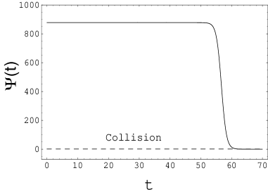
Figure 2: Evolution of the radion in the induced metric frame is depicted for the parameters $\alpha=0.98,\beta_{1}=1.000001,\beta_{2}=0.005$. For these parameters, Hubble parameter becomes 1.2413 in unit of $1/\ell_{I}$, the number of e-foldings becomes about 74.

When $\Psi$ reaches $1$, the inflation is suddenly terminated by the collision of branes in our scenario.

III.2 View from the Einstein frame

We have shown that we can obtain a de Sitter inflationary universe in the induced metric frame due to the existence of the flux between the two branes in the bulk. It is interesting to see this in the conformally related Einstein frame nojiri . In the Einstein frame, the metric is $\gamma_{\mu\nu}=[\Psi^{2}+(\alpha-1)]~{}h_{\mu\nu}$, using the variable $\Psi^{2}=(1-\alpha)\coth^{2}\psi$. Then the action reduces to

$$S = \frac{\ell_{I}}{2\kappa^{2}}\int d^{4}x\sqrt{-\gamma}\left[R(\gamma)-6\left(\partial\psi\right)^{2}-U(\psi)\right]$$ (16)

where the effective potential for the minimally-coupled radion $\psi$ is given by

$$\frac{\ell_{I}^{2}}{12}U=\left(\beta_{1}-1\right)\cosh^{4}\psi-\frac{\frac{1}{\alpha}-1-\beta_{2}}{(1-\alpha)^{2}}\sinh^{4}\psi\ .$$ (17)

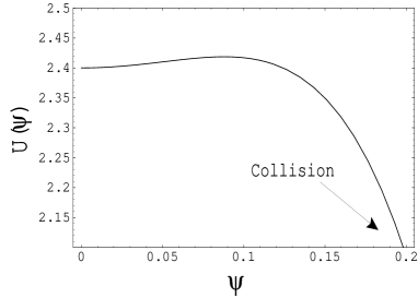
Figure 3: Here, we present the radion potential. The collision point is determined by $\coth^{2}\psi=1/\sqrt{1-\alpha}$.

The above potential is depicted in Figure 3. The unstable extremum corresponds to the static two de Sitter brane solution.

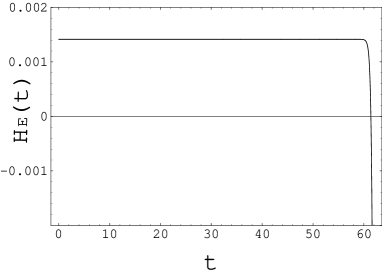
Figure 4: Evolution of the Hubble parameter in the Einstein frame for the same parameters as Figure 2. The horizontal axis represents the cosmic time in Jordan frame.

This extremum is located at $\psi_{0}$ determined by

$$(\beta_{1}-1)\cosh^{2}\psi_{0}=\frac{\frac{1}{\alpha}-1-\beta_{2}}{(1-\alpha)^{2}}\sinh^{2}\psi_{0}\ .$$ (18)

In that case, the potential energy becomes

$$\frac{\ell_{I}^{2}}{12}U\big{|}_{\psi=\psi_{0}}=\frac{\frac{1}{\alpha}-1-\beta_{2}}{(1-\alpha)^{2}}\sinh^{2}\psi_{0}\ .$$ (19)

The effective mass-squared is negative,

$$\frac{\ell_{I}^{2}}{12}\frac{d^{2}U}{d\psi^{2}}\Big{|}_{\psi=\psi_{0}}=-8\frac{\frac{1}{\alpha}-1-\beta_{2}}{(1-\alpha)^{2}}\sinh^{2}\psi_{0}\ .$$ (20)

From the above, one can read off the radion effective mass $m^{2}_{r}=-4H_{0}^{2}$, where $H_{0}$ represents the Hubble parameter at $\psi_{0}$. This indicates the linearised instability of the static two de Sitter brane system, consistent with previous analyses GenSas ; CF ; Contaldi .

Let us assume two branes are separated enough initially, which means the radion is located at near the maximum. The radion then starts to roll down the hill and reaches the collision point $\coth^{2}\psi=1/\sqrt{1-\alpha}$ which corresponds to $\Psi=1$. In contrast to the other models discussing collisions Khoury ; Gen ; Bucher ; KSS ; GT ; Pillado , our model has no singularity at the collision because the bulk region never disappears in our model.

The Hubble parameter in the Einstein frame, $H_{E}$, is related to the Hubble parameter in the induced metric frame, $H_{2}$, as

$$H_{E}=\frac{1}{\sqrt{\Psi^{2}-1+\alpha}}H_{2}+\frac{\Psi\dot{\Psi}}{\left(\Psi^{2}-1+\alpha\right)^{3/2}}\ .$$ (21)

The typical behavior of the Hubble parameter in the Einstein frame is depicted in Figure 4. While $\Psi$ remains almost constant the Hubble rate is also nearly constant and we have almost exponential expansion in both the induced and Einstein frames. Due to the suppression factor $1/\sqrt{\Psi^{2}-1+\alpha}$, the Hubble rate in the Einstein frame is much smaller than that in the induced frame. However, the e-folding number is almost the same as that in the Jordan frame because the time in the Einstein frame becomes longer by the conformal factor $\sqrt{\Psi^{2}+(\alpha-1)}$. Shortly before the collision, we find that the effective potential in the Einstein frame becomes negative, the universe recollapses and immediately before the collision the universe is contracting in the Einstein frame, though the universe is always expanding in the induced metric frame.

III.3 Graceful Exit Through Brane Collision

We need a fully 5-dimensional consideration to give a rule for evolution through the collision. We consider the simplest case of a completely inelastic collision where the bulk brane is absorbed by the boundary brane.

To describe the $Z_{2}$-symmetric collision of the branes it is useful to consider the complete system of four branes, consisting of the incoming $Z_{2}$ symmetric boundary brane, two copies of the bulk brane, and the outgoing $Z_{2}$ symmetric brane (see Figure 5).

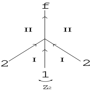
Figure 5: The collision process is schematically depicted. The final brane has also $Z_{2}$ symmetry.

A detailed analysis gives consistency conditions for the collision Neronov ; LMW . These are equivalent to relativistic energy-momentum conservation LMW

$$\rho_{f}=\sigma_{1}+2\gamma_{2|1}\sigma_{2}$$ (22)

where the pseudo-Lorentz factor between the colliding branes can be written as $\gamma_{2|1}\equiv\cosh(\theta_{2}-\theta_{1})$ where

$$\sinh\theta_{1}=H_{1}\ell_{1}\,,\quad\sinh\theta_{2}=H_{2}\ell_{1}\,.$$ (23)

At low energy (small “angles”) this reduces to the “Newtonian” energy conservation law

$$\rho_{f}=\sigma_{1}+2\sigma_{2}\,,$$ (24)

plus the momentum conservation law

$$H_{f}=\frac{1}{\alpha}\left[H_{1}-(1-\alpha)H_{2}\right]\ .$$ (25)

Hence, in order to obtain an expanding universe after the collision we have to impose the constraint

$$H_{1}>(1-\alpha)H_{2}\,.$$ (26)

In addition to this constraint, we require that the expansion rate of the bulk brane is bigger than the $Z_{2}$ symmetric brane, $H_{2}>H_{1}$, in order to cause a collision. It is easy to meet both these requirements, as we set $\alpha<1$.

III.4 Cosmological Evolution After the Collision

After the collision, we assume the branes coalesce and behave as a single brane. We further assume the resulting brane tension is given by the RS value, $\kappa^{2}\sigma_{f}=6/\ell_{II}$ so that the effective cosmological constant on the brane vanishes after the collision. This is the brane-world equivalent of the usual assumption that the inflaton potential is zero at its minimum.

At the collision, the additional energy density (above the RS brane tension) is assumed to be transferred to light degrees of freedom on the brane, i.e., radiation. Hence, the subsequent evolution will be governed by the standard Friedmann equation for the hot big bang with small Kaluza-Klein corrections.

As the radion disappears after the collision, the difference between the induced metric frame and the Einstein frame also disappears. In the Einstein frame, the abrupt change of the contracting phase to the expanding phase cannot be described within the 4-dimensional effective theory. This clearly shows that our model is different from a conventional 4-dimensional inflationary model.

IV Perturbations

Having constructed a homogeneous cosmological model, we can now consider the spectrum of inhomogeneous perturbations that would be expected due to small-scale quantum fluctuations. As there is no singularity at the collision, we can unambiguously follow the evolution of fluctuations generated during inflation through the collision.

To study the behavior of fluctuations before the collision, it is convenient to work in the Einstein frame in which the radion is minimally coupled to the metric. We have the equations of motion in the Einstein frame

$$G_{\mu\nu}=6\left(\partial_{\mu}\psi\partial_{\nu}\psi-\frac{1}{2}\gamma_{\mu\nu}(\partial\psi)^{2}\right)-\frac{1}{2}\gamma_{\mu\nu}U(\psi)$$

$$\Box\psi-\frac{1}{12}\frac{dU}{d\psi}=0\ .$$ (27)

The homogeneous and istropic background metric is

$$ds^{2}=b^{2}(\eta)\left[-d\eta^{2}+\delta_{ij}dx^{i}dx^{j}\right]\ .$$ (28)

and we have the Einstein equations become

$$3{\cal H}^{2}=3\psi^{\prime 2}+\frac{1}{2}b^{2}U(\psi)$$ (29)

$${\cal H}^{2}+2{\cal H}^{\prime}=-3\psi^{\prime 2}+\frac{1}{2}b^{2}U(\psi)$$ (30)

$$\psi^{\prime\prime}+2{\cal H}\psi^{\prime}+\frac{b^{2}}{12}\frac{\partial U}{\partial\psi}=0\ .$$ (31)

where a prime denotes a derivative with respect to the conformal time $\eta$ and ${\cal H}=b^{\prime}/b$. During the de Sitter phase, the solution is

$$b=\frac{1}{-H_{0}\eta}\ ,\quad\psi=\psi_{0}\ ,$$ (32)

where $bH_{0}={\cal H}_{0}$ and

$$\ell_{I}^{2}H_{0}^{2}=2\frac{\frac{1}{\alpha}-1-\beta_{2}}{(1-\alpha)^{2}}\sinh^{2}\psi_{0}\ .$$ (33)

Now we can examine possible fluctuations separately.

IV.1 Gravitational waves

Let us consider first the tensor perturbations

$$ds^{2}=b^{2}(\eta)\left[-d\eta^{2}+\left(\delta_{ij}+q_{ij}\right)dx^{i}dx^{j}\right]\ ,$$ (34)

where the tensor perturbations satisfy $q^{i}{}_{i}=0\ ,\ q_{ij,j}=0$. We can reduce the Einstein equations to

$$q_{ij}^{\prime\prime}+2{\cal H}q_{ij}^{\prime}+k^{2}q_{ij}=0\ .$$ (35)

Before the radion starts to roll down the hill, the background spacetime is the de Sitter spacetime (32). The positive frequency mode function is the standard one

$$q_{ij}\propto(-H_{0}\eta)^{3/2}H^{(1)}_{3/2}(-k\eta)\ ,$$ (36)

where $H^{(1)}_{3/2}$ is the Hankel’s function of the first kind. This gives the standard flat spectrum for the primordial gravitational waves. During the roll down phase, the universe will begin to contract rapidly from a numerical calculation, we see that the contracting phase is negligible in practice. During the collision process, as the gravitational waves are independent of gauge, we will have a flat spectrum on long wavelengths after the collision when the standard radiation dominated era begins.

IV.2 Radion fluctuations

To study the behavior of the radion fluctuations, we express the metric perturbation in the Einstein frame as

$$ds^{2}=b^{2}\left[-(1+2A)d\eta^{2}+2\partial_{i}Bdx^{i}d\eta\right.$$

$$\qquad\qquad\left.+\left((1+2{\cal R})\delta_{ij}+2\partial_{i}\partial_{j}E\right)dx^{i}dx^{j}\right]\ ,$$ (37)

where $A,B,{\cal R},E$ represent the gauge-dependent scalar metric perturbations. A convenient gauge-invariant combination is the comoving curvature perturbation, which is the intrinsic curvature perturbation on uniform-radion hypersurfaces:

$${\cal R}_{c}={\cal R}-{\cal H}{\delta\psi\over\psi^{\prime}}\,.$$ (38)

The second-order action for the curvature perturbation ${\cal R}_{c}$ is

$$S={1\over 2}\int d\eta\,d^{3}x\,z^{2}\left[{\cal R}_{c}^{\prime}{}^{2}-{\cal R}_{c}^{\,|i}{\cal R}_{c\,|i}\right]\,,$$ (39)

where

$$z=\sqrt{3\ell_{I}\over 2\kappa^{2}}\,{b\psi^{\prime}\over{\cal H}}\,.$$ (40)

The equation of motion for ${\cal R}_{c}$ is

$${\cal R}_{c}^{\prime\prime}+2{z^{\prime}\over z}{\cal R}_{c}^{\prime}+k^{2}{\cal R}_{c}=0\ .$$ (41)

Therefore, on large scales, ${\cal R}_{c}$ is constant.

Equivalently we can work in terms of the radion on uniform-curvature hypersurfaces

$$Q=\delta\psi-\frac{\psi^{\prime}}{{\cal H}}{\cal R}=-\frac{\psi^{\prime}}{{\cal H}}{\cal R}_{c}\,.$$ (42)

During the de Sitter phase, the equation for $Q$ can be written as

$$Q^{\prime\prime}+2{\cal H}Q^{\prime}+(k^{2}-4H_{0}^{2}b^{2})Q=0\ ,$$ (43)

where we have used Eq. (31). Hence, the positive frequency mode becomes

$$Q\sim(-H_{0}\eta)^{3/2}H^{(1)}_{5/2}(-k\eta)\ ,$$ (44)

where $H^{(1)}_{5/2}$ is the Hankel’s function of the first kind. Thus, we can read off the power spectrum of $Q$ as ${\cal P}_{Q}\sim k^{-2}$. Despite the exponential expansion the spectrum on large scales becomes red during the de Sitter inflation because the radion has negative effective mass-squared.

These field fluctuations can be translated to the curvature perturbations on comoving hypersurfaces via Eq. (42). The coefficient $\psi^{\prime}/{\cal H}$ is independent of scale and hence the comoving curvature perturbation shares the same red spectrum, ${\cal P}_{\cal R}\sim k^{-2}$. Near the collision, we expect the spectrum to be blue because of the rapid contraction, but this only affects small scales.

Finally, we need to calculate the curvature perturbation on uniform-density hypersurfaces, $\zeta$, on large scales after the collision. This should then remain constant on large scales for adiabatic perturbations after the collision, even in the brane-world Langlois , simply as a consequence of local energy conservation WMLL .

In the low-energy limit, energy conservation at the collision gives Eq. (24) which implies that the collision hypersurface will be a uniform-energy hypersurface. Thus $\zeta$ after the collision coincides with the curvature perturbation of this collision hypersurface.

We define the collision hypersurface in terms of the low-energy effective theory before the collision by the condition that $\Psi=1$. Thus the collision hypersurface is a uniform-radion hypersurface and we can identify the curvature perturbation on this hypersurface as the comoving curvature perturbation, $\zeta=-{\cal R}_{c}$ (where the negative sign comes from different historical conventions for the sign of the curvature perturbation).

One might worry that ${\cal R}_{c}$ was calculated in the Einstein frame and the collision hypersurface corresponds to a physical hypersurface on the two branes. In fact the comoving curvature perturbation is invariant under any conformal transformation that is function of the radion field, $\Omega^{2}(\Psi)$, as the conformal transformation then corresponds to a uniform rescaling on uniform-$\Psi$ hypersurfaces, leaving the comoving curvature perturbation conformally invariant. Hence ${\cal R}_{c}$ does describe the curvature perturbation on the physical collision hypersurface.

Alternatively we can calculate the curvature perturbation on the collision hypersurface using the $\delta N$ formalism Sasaki . This says that the curvature perturbation is given by the perturbed expansion with respect to an initial flat hypersurface, or $\zeta=(dN/d\phi_{*})\delta\phi_{*}$ where $\delta\phi_{*}$ is the field perturbation on the initial spatially flat hypersurface at horizon exit. This gives the usual expression ${\cal R}_{c}=-(H/\dot{\psi})Q$ for the comoving curvature perturbation during inflation. Because the collision hypersurface is a uniform-$\psi$ hypersurface before the collision and a uniform-density hypersurface after the collision we have $\zeta=-{\cal R}_{c}=(H/\dot{\psi})Q$.

However, we have shown that the comoving curvature perturbation has a steeply tilted red spectrum which means that these perturbations cannot be responsible for the formation of the large scale structure in our Universe.

IV.3 Scale-invariant perturbations

The curvaton mechanism EnqSlo ; LW ; MT provides a simple example of how scale-invariant perturbations could be generated in our model. Both the bulk and boundary branes experience a de Sitter expansion before the collision. The radion field acquires a red spectrum due to its negative mass-squared, but any minimally-coupled, light scalar field living on either brane would acquire a scale-invariant spectrum of perturbations before the collision.

Thus we add to our basic model an additional degree of freedom which, to be specific, we assume lives on the bulk brane. The action for the curvaton $\chi$ in the induced metric frame takes the simple form

$$S_{\rm curvaton}=\int d^{4}x\sqrt{-h}\left[-\frac{1}{2}(\partial\chi)^{2}\right]$$ (45)

Vacuum fluctuations of a massless scalar field in de Sitter spacetime have the same time-dependence as the graviton (36), becoming frozen-in on large scales. Normalising to the Bunch-Davies vacuum state on small scales leads to the standard scale-invariant spectrum, $(H_{2}/2\pi)^{2}$, on super-Hubble scales. Hence, the fluctuations of the curvaton have a completely flat spectrum.

This is similar the way the curvaton mechanism was originally proposed in the pre-big bang scenario EnqSlo ; LW where axion fields have a non-trivial coupling to the dilaton field in the Einstein frame, but are minimally coupled in a conformally related frame, which can give rise to a scale-invariant spectrum if the expansion is de Sitter in that conformal frame CEW .

The curvaton mechanism requires that the curvaton has a non-zero mass after the collision, which seems entirely natural if the collision is associated with some symmetry-breaking in the degrees of freedom on the brane. The energy density of any massive scalar field will grow relative to the radiation density once the Hubble rate drops below its effective mass. Indeed the particles must decay before primordial nucleosynthesis to avoid an early matter domination in conflict with standard predictions of the abundances of the light elements. But if the curvaton comes to contribute a significant fraction of the total energy density before it decays then perturbations in the curvaton will result in primordial density perturbations on large scales capable of seeding the large scale structure in our Universe EnqSlo ; LW ; MT .

V Conclusions

We have proposed a geometrical model of inflation where inflation on two branes is driven by the flux generated by the brane charge and terminated by the brane collision with charge annihilation. We assume the collision process is completely inelastic and the kinetic energy is transformed into the thermal energy. After the collision the two branes coalesce together and behave as a single brane universe with zero effective cosmological constant.

The four-dimensional, low-energy effective theory in the Einstein frame has to change abruptly at the collision point. Therefore, our model needs to be consistently described using 5-dimensional gravity. This can be done using consistency conditions at the collision that ensure energy-momentum conservation in the 5-dimensional theory. As the collision process has no singularity in the 5-dimensional gravity, we can unambiguously follow the evolution of inhomogeneous vacuum fluctuations about this homogenous background during the whole history of the universe. It turns out that the radion fluctuations produced during inflation have a steep red spectrum and cannot produce the present large-scale structure of our universe. Instead the curvature perturbations observed today must be generated by the curvaton or some similar mechanism from initially isocurvature excitations of massless degrees of freedom on one or other of the branes before the collision. The primordial gravitational waves produced are likely to be difficult to detect.

Our model does suffer from a significant fine tuning problem of the initial conditions. The radion field must start very close to an unstable extremum of its potential in order to obtain sufficient inflation. However, the radion field has a geometrical meaning so that the initial value is determined by the initial separation between two branes. Sufficient separation of the initial brane positions does not seem so unnatural, and the fine tuning valu of the radion may not be so serious. A quantum cosmological consideration GS ; Koyama would be needed to give a more insight on this initial condition problem. It might be that one can find an instanton solution to describe tunnelling to this extremum. Alternatively, in a semi-classical model such as stochastic inflation, it may be that quantum fluctuations drive the field to the top of the potential before classical evolution takes over and the field rolls down, leading to the branes to collide.

We stress that our model is fundamentally 5-dimensional in nature. It cannot be constructed starting from a 4-dimensional theory. It would of course be interesting to see if it is possible to embed our model into string theory model, but that goes beyond the scope of this paper.

Note added: While this work was being written up Koyama and Koyama KKKK submitted a related paper deriving an equivalent effective action for anti-D-branes in a type IIB string model.

Appendix A Derivation of effective action

A.1 Static Solution

We shall start with the three-brane system and take the two-brane limit to derive the low energy effective action for the two-brane system. This allows us to use a simple moduli approximation method. Assuming there exists no matter on the third brane, this procedure can be justified.

In the low energy limit, the configuration should be almost static. As we have no matter in the bulk, the bulk metric should be anti-de Sitter spacetime. Hence, let us first consider the static solution of the form

$$ds_{I}^{2}=dy^{2}+b_{I}^{2}(y)\eta_{\mu\nu}dx^{\mu}dx^{\nu}$$

$$ds_{I\!I}^{2}=dy^{2}+b_{I\!I}^{2}(y)\eta_{\mu\nu}dx^{\mu}dx^{\nu}$$ (46)

where $b_{I}=\exp(-y/\ell_{I})$ and $b_{I\!I}=\exp(-y/\ell_{I\!I})$ represents the warp factor in each region. The bulk equation of motion imply the relation between the curvature scale in the bulk and the flux as

$$\frac{6}{\ell_{I}^{2}}=\Lambda-\frac{\kappa^{2}}{2}c_{I}^{2}\ ,$$

$$\frac{6}{\ell_{I\!I}^{2}}=\Lambda-\frac{\kappa^{2}}{2}c_{I\!I}^{2}\ .$$ (47)

We also have junction conditions for the metric which give the relation

$$\kappa^{2}\sigma_{1}=\frac{6}{\ell_{I}}$$ (48)

$$\kappa^{2}\sigma_{2}=\frac{3}{\ell_{I\!I}}-\frac{3}{\ell_{I}}$$ (49)

$$\kappa^{2}\sigma_{3}=-\frac{6}{\ell_{I\!I}}\ .$$ (50)

If we assume the inflating bulk brane $\sigma_{2}>0$, we have $\ell_{I\!I}<\ell_{I}$. The above implies the relation

$$\sigma_{1}+2\sigma_{2}+\sigma_{3}=0\ .$$ (51)

The junction conditions for 5-form fields give

$$c_{I}=-\frac{\mu_{1}}{2}\ ,\quad c_{I\!I}=-(\mu_{2}+\frac{\mu_{1}}{2})$$ (52)

$$\mu_{1}+2\mu_{2}+\mu_{3}=0\ .$$ (53)

The last relation is nothing but the charge conservation law. The static solution is realized under the relations Eqs. (51) and (53). In this paper, we set $\mu_{3}=0$. This implies $c_{I\!I}=0$.

A.2 Low energy effective action

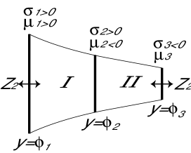
Figure 6: three-brane system

Let us employ the moduli approximation method GPT which can be shown to be valid at low energy Soda ; Kanno . (An alternative derivation appears in Ref. Ludo .) In this method, we can use the factorized metric ansatz

$$ds^{2} = dy^{2}+b_{I}^{2}(y)g_{\mu\nu}^{I}(x)dx^{\mu}dx^{\nu}$$

$$ds^{2} = dy^{2}+b_{I\!I}^{2}(y)g_{\mu\nu}^{I\!I}(x)dx^{\mu}dx^{\nu}\ .$$ (54)

The brane positions are denoted by $\phi_{1}(x),\phi_{2}(x)$ and $\phi_{3}(x)$. Now, we calculate the bulk action, the action for each brane tensions, and the Gibbons-Hawking terms, separately.

Let us start with the calculation of the bulk action. For the metric (54), using the Gauss equation, it is straightforward to relate the bulk Ricci scalar to the 4-dimentional Ricci scalar,

$$\overset{(5)}{R}=\frac{R(g^{i})}{b_{i}^{2}}-\frac{20}{\ell_{i}^{2}}\ ,$$ (55)

we can write the contributions from each bulk as

$$S_{\rm bulkI} = \frac{2}{2\kappa^{2}}\int d^{4}x\sqrt{-g^{I}}\int^{\phi_{2}}_{\phi_{1}}dyb_{I}^{4}(y)\left[\frac{R(g^{I})}{b_{I}^{2}}-\frac{8}{\ell_{I}^{2}}\right]$$ (56)

$$= \frac{1}{\kappa^{2}}\int d^{4}x\sqrt{-g^{I}}\left[-\frac{\ell_{I}}{2}\left\{b_{I}^{2}(\phi_{2})-b_{I}^{2}(\phi_{1})\right\}R(g^{I})\right.$$

$$\left.+\frac{2}{\ell_{I}}\left\{b_{I}^{4}(\phi_{2})-b_{I}^{4}(\phi_{1})\right\}\right]$$

where we used the bulk equation of motion (47) in the first line. The factor 2 over $\kappa^{2}$ comes from the $Z_{2}$ symmetry of this spacetime and we neglected the second order quantities. In the same way for region II, we have

$$S_{\rm bulkI\!I}=\frac{2}{2\kappa^{2}}\int d^{4}x\sqrt{-g^{I\!I}}\int^{\phi_{3}}_{\phi_{2}}dyb_{I\!I}^{4}(y)\left[\frac{R(g^{II})}{b_{I\!I}^{2}}-\frac{8}{\ell_{I\!I}^{2}}\right]$$

$$=\frac{1}{\kappa^{2}}\int d^{4}x\sqrt{-g^{I\!I}}\left[-\frac{\ell_{I\!I}}{2}\left\{b_{I\!I}^{2}(\phi_{3})-b_{I\!I}^{2}(\phi_{2})\right\}R(g^{II})\right.$$

$$\left.\qquad+\frac{2}{\ell_{I\!I}}\left\{b_{I\!I}^{4}(\phi_{3})-b_{I\!I}^{4}(\phi_{2})\right\}\right]\ .$$ (57)

In order to calculate the action for each brane tensions, we need to know the induced metric. The induced metric on the left boundary brane becomes

$$b^{2}(\phi_{1})g_{\mu\nu}^{I}+\partial_{\mu}\phi_{1}\partial_{\nu}\phi_{1}$$ (58)

and the similar formula holds for other branes. Then, the contributions from the brane tension terms become

$$S_{1}=-\sigma_{1}\int d^{4}x\sqrt{-g^{I}}b_{I}^{4}(\phi_{1})\left[1+\frac{1}{2b_{I}^{2}(\phi_{1})}\left(\partial\phi_{1}\right)^{2}\right]\ ,\quad$$ (59)

$$S_{2} = -2\sigma_{2}\int d^{4}x\sqrt{-g^{I}}b_{I}^{4}(\phi_{2})\left[1+\frac{1}{2b_{I}^{2}(\phi_{2})}\left(\partial\phi_{2}\right)^{2}\right]$$ (60)

$$= \!\!\!\!-2\sigma_{2}\int d^{4}x\sqrt{-g^{I\!I}}b_{I\!I}^{4}(\phi_{2})\left[1+\frac{1}{2b_{I\!I}^{2}(\phi_{2})}\left(\partial\phi_{2}\right)^{2}\right]\qquad\quad$$

and

$$S_{3}=-\sigma_{3}\int d^{4}x\sqrt{-g^{I\!I}}b_{I\!I}^{4}(\phi_{3})\left[1+\frac{1}{2b_{I\!I}^{2}(\phi_{3})}\left(\partial\phi_{3}\right)^{2}\right]\ ,\quad$$ (61)

where the factor 2 in front of $\sigma_{2}$ comes from the $Z_{2}$ symmetry.

Let us turn to the calculation of Gibbons-Hawking terms. The extrinsic curvature in leading order is given by

$$K_{\mu\nu}=n_{y}\left[\frac{4}{\ell}+\frac{1}{b^{2}}\Box\phi+\frac{1}{\ell b^{2}}(\partial\phi)^{2}\right]\ ,$$ (62)

where $n_{y}$ is the normal vector to the brane defined by

$$n_{y}=\left(1+\frac{1}{b^{2}}(\partial\phi)^{2}\right)^{-1/2}\ .$$ (63)

Hence, the Gibbons-Hawking terms are

$$S_{\scriptscriptstyle\rm GH1}=\frac{2}{\kappa^{2}\ell_{I}}\int d^{4}x\sqrt{-g^{I}}\left[4b_{I}^{4}(\phi_{1})+3b_{I}^{2}(\phi_{1})\left(\partial\phi_{1}\right)^{2}\right]\ ,\ \quad$$ (64)

$$S_{\scriptscriptstyle\rm GH2}=\frac{2}{\kappa^{2}\ell_{I\!I}}\int d^{4}x\sqrt{-g^{I\!I}}\left[4b_{I\!I}^{4}(\phi_{2})+3b_{I\!I}^{2}(\phi_{2})\left(\partial\phi_{2}\right)^{2}\right]$$

$$-\frac{2}{\kappa^{2}\ell_{I}}\int d^{4}x\sqrt{-g^{I}}\left[4b_{I}^{4}(\phi_{2})+3b_{I}^{2}(\phi_{2})\left(\partial\phi_{2}\right)^{2}\right]\ ,\qquad$$ (65)

and

$$S_{\scriptscriptstyle\rm GH3}=\frac{2}{\kappa^{2}\ell_{I\!I}}\int d^{4}x\sqrt{-g^{I\!I}}\left[4b_{I\!I}^{4}(\phi_{3})+3b_{I\!I}^{2}(\phi_{3})\left(\partial\phi_{3}\right)^{2}\right]\ ,\ \$$ (66)

where the factor 2 over $\kappa^{2}$ in $S_{\rm GH2}$ again comes from the $Z_{2}$ symmetry

Substituting Eqs.(56), (57), (59), (60) (61), (64), (65) and (66) into the 5-dimensional action (1), the resultant 4-dimensional effective action can be summarized by the following. The curvature part becomes

$$S_{\rm R}=\frac{\ell_{I}}{2\kappa^{2}}\int d^{4}x\sqrt{-g^{I}}\left[b_{I}^{2}(\phi_{1})-b_{I}^{2}(\phi_{2})\right]R(g^{I})$$

$$+\frac{\ell_{I\!I}}{2\kappa^{2}}\int d^{4}x\sqrt{-g^{I\!I}}\left[b_{I\!I}^{2}(\phi_{2})-b_{I\!I}^{2}(\phi_{3})\right]R(g^{I\!I})\ .\quad$$ (67)

The kinetic part of radions are

$$S_{\rm K}=\frac{3}{\kappa^{2}\ell_{I}}\int d^{4}x\sqrt{-g^{I}}\left[b_{I}^{2}(\phi_{1})\left(\partial\phi_{1}\right)^{2}-b_{I}^{2}(\phi_{2})\left(\partial\phi_{2}\right)^{2}\right]$$

$$+\frac{3}{\kappa^{2}\ell_{I\!I}}\int d^{4}x\sqrt{-g^{I\!I}}\left[b_{I\!I}^{2}(\phi_{2})\left(\partial\phi_{2}\right)^{2}-b_{I\!I}^{2}(\phi_{3})\left(\partial\phi_{3}\right)^{2}\right]\ .\qquad$$ (68)

The potential energy will be induced as

$$S_{\rm V}=\int d^{4}x\sqrt{-g^{I}}\left[\left(\frac{6}{\kappa^{2}\ell_{I}}-\sigma_{1}\right)b_{I}^{4}(\phi_{1})\right.$$

$$\left.-\left\{2\sigma_{2}-\frac{6}{\kappa^{2}}\left(\frac{1}{\ell_{I\!I}}-\frac{1}{\ell_{I}}\right)\right\}b_{I}^{4}(\phi_{2})\right]$$

$$-\int d^{4}x\sqrt{-g^{I\!I}}\left(\sigma_{3}+\frac{6}{\kappa^{2}\ell_{I\!I}}\right)b_{I\!I}^{4}(\phi_{3})\ .$$ (69)

Now we can write down the effective action for the bulk brane. The continuity condition of the metric is given by

$$h_{\mu\nu}=b_{I}^{2}(\phi_{2})g^{I}_{\mu\nu}=b_{I\!I}^{2}(\phi_{2})g^{I\!I}_{\mu\nu}\ ,$$ (70)

where $h_{\mu\nu}$ is the induced metric of the bulk brane. Defining the variables

$$\Psi=\frac{b_{I}(\phi_{1})}{b_{I}(\phi_{2})}\ ,\quad\Phi=\frac{b_{I\!I}(\phi_{3})}{b_{I\!I}(\phi_{2})}\ ,$$ (71)

we obtain

$$S = \frac{\ell_{I}}{2\kappa^{2}}\int d^{4}x\sqrt{-h}\left[\Psi^{2}-1+\alpha\left(1-\Phi^{2}\right)\right]R(h)$$ (72)

$$+\frac{3\ell_{I}}{\kappa^{2}}\int d^{4}x\sqrt{-h}\left[\left(\partial\Psi\right)^{2}-\alpha\left(\partial\Phi\right)^{2}\right]$$

$$+\frac{6}{\kappa^{2}\ell_{I}}\int d^{4}x\sqrt{-h}\left[\left(1-\beta_{1}\right)\Psi^{4}\right.$$

$$\left.-\left(1-\frac{1}{\alpha}+\beta_{2}\right)-\left(\frac{1}{\alpha}+\beta_{3}\right)\Phi^{4}\right]\ .$$

Here we have defined the dimensionless parameters

$$\alpha=\frac{\ell_{I\!I}}{\ell_{I}}\ ,$$ (73)

$$\beta_{1}=\frac{\kappa^{2}\sigma_{1}\ell_{I}}{6}\ ,\quad\beta_{2}=\frac{\kappa^{2}\sigma_{2}\ell_{I}}{3}\ ,\quad\beta_{3}=\frac{\kappa^{2}\sigma_{3}\ell_{I}}{6}\ .$$ (74)

As we have the relation $\ell_{I\!I}<\ell_{I}$, the relation $\alpha<1$ also holds.

After taking the two-brane limit $a(\phi_{3})\rightarrow 0$, namely, $\Phi\rightarrow 0$, we obtain the low energy effective action for the two-brane system.

$$S=\frac{\ell_{I}}{2\kappa^{2}}\int d^{4}x\sqrt{-h}\left(\Psi^{2}+\alpha-1\right)R(h)$$

$$\quad+\frac{3\ell_{I}}{\kappa^{2}}\int d^{4}x\sqrt{-h}\left(\partial\Psi\right)^{2}$$ (75)

$$+\frac{6}{\kappa^{2}\ell_{I}}\int d^{4}x\sqrt{-h}\left[\left(1-\beta_{1}\right)\Psi^{4}-\left(1-\frac{1}{\alpha}+\beta_{2}\right)\right]\ .$$

The scalar variable $\Psi$ which describes the distance between two positive tension branes is called as the radion.

References

- (1) P. Horava and E. Witten, Nucl. Phys. B 460, 506 (1996) [arXiv:hep-th/9510209]; I. Antoniadis, N. Arkani-Hamed, S. Dimopoulos and G. R. Dvali, Phys. Lett. B 436, 257 (1998) [arXiv:hep-ph/9804398]; A. Lukas, B. A. Ovrut, K. S. Stelle and D. Waldram, Phys. Rev. D 59, 086001 (1999) [arXiv:hep-th/9803235]; N. Arkani-Hamed, S. Dimopoulos and G. R. Dvali, Phys. Lett. B 429, 263 (1998) [arXiv:hep-ph/9803315].
- (2) G. R. Dvali and S. H. H. Tye, Phys. Lett. B 450, 72 (1999) [arXiv:hep-ph/9812483].
-
(3)
S. Kachru, R. Kallosh, A. Linde and S. P. Trivedi,
Phys. Rev. D 68, 046005 (2003)
[arXiv:hep-th/0301240];
S. Kachru, R. Kallosh, A. Linde, J. Maldacena, L. McAllister and S. P. Trivedi, JCAP 0310, 013 (2003) [arXiv:hep-th/0308055]; - (4) R. Maartens, Living Rev. Rel. 7, 7 (2004) [arXiv:gr-qc/0312059]; P. Brax, C. van de Bruck and A. C. Davis, Rept. Prog. Phys. 67, 2183 (2004) [arXiv:hep-th/0404011]; S. Kanno and J. Soda, arXiv:hep-th/0407184.
- (5) R. Maartens, D. Wands, B. A. Bassett and I. Heard, Phys. Rev. D 62, 041301 (2000) [arXiv:hep-ph/9912464].
- (6) D. Langlois, R. Maartens and D. Wands, Phys. Lett. B 489, 259 (2000) [arXiv:hep-th/0006007].
- (7) S. Kobayashi, K. Koyama and J. Soda, Phys. Lett. B 501, 157 (2001) [arXiv:hep-th/0009160].
- (8) Y. Himemoto and M. Sasaki, Phys. Rev. D 63, 044015 (2001) [arXiv:gr-qc/0010035].
- (9) L. Randall and R. Sundrum, Phys. Rev. Lett. 83, 3370 (1999) [arXiv:hep-ph/9905221];
- (10) S. Kanno and J. Soda, Phys. Rev. D 66, 083506 (2002) [arXiv:hep-th/0207029];
-
(11)
S. Kanno and J. Soda,
Phys. Rev. D 66, 043526 (2002)
[arXiv:hep-th/0205188];
S. Kanno and J. Soda, Astrophys. Space Sci. 283, 481 (2003) [arXiv:gr-qc/0209087];
S. Kanno and J. Soda, Gen. Rel. Grav. 36, 689 (2004) [arXiv:hep-th/0303203]. -
(12)
T. Wiseman,
Class. Quant. Grav. 19, 3083 (2002)
[arXiv:hep-th/0201127];
T. Shiromizu and K. Koyama, Phys. Rev. D 67, 084022 (2003) [arXiv:hep-th/0210066]. - (13) D. Langlois, K. Maeda and D. Wands, Phys. Rev. Lett. 88, 181301 (2002) [arXiv:gr-qc/0111013].
- (14) T. Shiromizu, K. Koyama and T. Torii, Phys. Rev. D 68, 103513 (2003) [arXiv:hep-th/0307151]; K. Takahashi and T. Shiromizu, Phys. Rev. D 70, 103507 (2004) [arXiv:hep-th/0408043]; P. Brax and N. Chatillon, JHEP 0312, 026 (2003) [arXiv:hep-th/0309117]; P. Brax and N. Chatillon, Phys. Rev. D 70, 106009 (2004) [arXiv:hep-th/0405143].
- (15) P. Binetruy, C. Deffayet and D. Langlois, Nucl. Phys. B 615, 219 (2001) [arXiv:hep-th/0101234].
- (16) N. Kaloper, Phys. Rev. D 60, 123506 (1999) [arXiv:hep-th/9905210].
- (17) P. Bowcock, C. Charmousis and R. Gregory, Class. Quant. Grav. 17, 4745 (2000) [arXiv:hep-th/0007177].
-
(18)
S. Kanno and J. Soda,
Phys. Lett. B 588, 203-209 (2004)
[arXiv:hep-th/0312106];
P. L. McFadden and N. Turok, Phys. Rev. D 71, 021901 (2005) [arXiv:hep-th/0409122]. - (19) L. Cotta-Ramusino, “Low energy effective theory for brane world models”, MPhil thesis, University of Portsmouth (2004).
- (20) T. Shiromizu, K. i. Maeda and M. Sasaki, Phys. Rev. D 62, 024012 (2000) [arXiv:gr-qc/9910076].
- (21) S. Nojiri, O. Obregon, S. D. Odintsov and V. I. Tkach, Phys. Rev. D 64, 043505 (2001) [arXiv:hep-th/0101003].
- (22) U. Gen and M. Sasaki, Prog. Theor. Phys. 105, 591 (2001) [arXiv:gr-qc/0011078].
- (23) Z. Chacko and P. J. Fox, Phys. Rev. D 64, 024015 (2001) [arXiv:hep-th/0102023].
- (24) C. R. Contaldi, L. Kofman and M. Peloso, JCAP 0408, 007 (2004) [arXiv:hep-th/0403270].
- (25) J. Khoury, B. A. Ovrut, P. J. Steinhardt and N. Turok, Phys. Rev. D 64, 123522 (2001) [arXiv:hep-th/0103239].
- (26) U. Gen, A. Ishibashi and T. Tanaka, Phys. Rev. D 66, 023519 (2002) [arXiv:hep-th/0110286].
- (27) M. Bucher, arXiv:hep-th/0107148.
- (28) S. Kanno, M. Sasaki and J. Soda, Prog. Theor. Phys. 109, 357 (2003) [arXiv:hep-th/0210250].
- (29) J. Garriga and T. Tanaka, Phys. Rev. D 65, 103506 (2002) [arXiv:hep-th/0112028].
- (30) J. J. Blanco-Pillado and M. Bucher, Phys. Rev. D 65, 083517 (2002) [arXiv:hep-th/0111089].
- (31) A. Neronov, JHEP 0111, 007 (2001) [arXiv:hep-th/0109090].
- (32) D. Langlois, R. Maartens, M. Sasaki and D. Wands, Phys. Rev. D 63, 084009 (2001) [arXiv:hep-th/0012044].
- (33) D. Wands, K. A. Malik, D. H. Lyth and A. R. Liddle, Phys. Rev. D 62, 043527 (2000) [arXiv:astro-ph/0003278].
- (34) M. Sasaki and E. D. Stewart, Prog. Theor. Phys. 95, 71 (1996) [arXiv:astro-ph/9507001].
- (35) K. Enqvist and M. S. Sloth, Nucl. Phys. B 626, 395 (2002) [arXiv:hep-ph/0109214].
- (36) D. H. Lyth and D. Wands, Phys. Lett. B 524, 5 (2002) [arXiv:hep-ph/0110002].
- (37) T. Moroi and T. Takahashi, Phys. Lett. B 522, 215 (2001) [Erratum-ibid. B 539, 303 (2002)] [arXiv:hep-ph/0110096].
- (38) E. J. Copeland, R. Easther and D. Wands, Phys. Rev. D 56, 874 (1997) [arXiv:hep-th/9701082].
- (39) J. Garriga and M. Sasaki, Phys. Rev. D 62, 043523 (2000) [arXiv:hep-th/9912118].
- (40) K. Koyama and J. Soda, Phys. Lett. B 483, 432 (2000) [arXiv:gr-qc/0001033].
- (41) K. Koyama and K. Koyama, arXiv:hep-th/0505256.
-
(42)
J. Garriga, O. Pujolas and T. Tanaka,
Nucl. Phys. B 655, 127 (2003)
[arXiv:hep-th/0111277];
P. Brax, C. van de Bruck, A. C. Davis and C. S. Rhodes, Phys. Rev. D 67, 023512 (2003) [arXiv:hep-th/0209158];
G. A. Palma and A. C. Davis, Phys. Rev. D 70, 106003 (2004) [arXiv:hep-th/0407036];
J. L. Lehners and K. S. Stelle, Nucl. Phys. B 661, 273 (2003) [arXiv:hep-th/0210228]. - (43) S. Kanno and J. Soda, Phys. Rev. D 71, 044031 (2005) [arXiv:hep-th/0410061].
- (44) S. Kanno, arXiv:hep-th/0504087.