Casimir Energies for 6D Supergravities Compactified on ${\cal T}_{2}/Z_{N}$ with Wilson Lines

Abstract:

We compute (as functions of the shape and Wilson-line moduli) the one-loop Casimir energy induced by higher-dimensional supergravities compactified from 6D to 4D on 2-tori, and on some of their $Z_{N}$ orbifolds. Detailed calculations are given for a 6D scalar field having an arbitrary 6D mass $m$, and we show how to extend these results to higher-spin fields for supersymmetric 6D theories. Particular attention is paid to regularization issues and to the identification of the divergences of the potential, as well as the dependence of the result on $m$, including limits for which $m^{2}{\cal A}\ll 1$ and $m^{2}{\cal A}\gg 1$ where ${\cal A}$ is the volume of the internal 2 dimensions. Our calculation extends those in the literature to very general boundary conditions for fields about the various cycles of these geometries. The results have potential applications towards Supersymmetric Large Extra Dimensions (SLED) as a theory of the Dark Energy. First, they provide an explicit calculation within which to follow the dependence of the result on the mass of the bulk states which travel within the loop, and for heavy masses these results bear out the more general analysis of the UV-sensitivity obtained using heat-kernel methods. Second, because the potentials we find describe the dynamics of the classical flat directions of these compactifications, within SLED they would describe the present-day dynamics of the Dark Energy.

1 Introduction.

The Casimir energy for various field theories compactified on 2 internal dimensions has been extensively studied (see for example refs. [1]-[16]). In this paper we return to this calculation for the particularly simple examples of 2-tori and their orbifolds. At the technical level, our aim in is to provide a generalization of previous calculations for fields compactified on ${\cal T}_{2}$ and ${\cal T}_{2}/Z_{N}$ to include very general boundary conditions, including those which would be generated by (constant) Wilson-line backgrounds.

Our physical motivation for performing this calculation is due to its relevance for the recent proposal for using 6D supergravity to shed light on the cosmological-constant problem [17, 18] within the context of Supersymmetric Large Extra Dimensions (SLED). (See also [19] for related discussions and similar proposals.) Within this proposal the extra dimensions must presently be sub-millimeter in size, and the recently-discovered [20] cosmological Dark Energy density corresponds to the Casimir energy of the model’s bulk fields as functions of the moduli of these large 2 internal dimensions. The smallness of the Dark Energy density in this picture is ultimately traced to the large size of these extra dimensions. In this picture these moduli can be extremely light in a technically natural way, and so the Dark Energy phenomenology is controlled by the dynamics of the moduli as they respond to this Casimir energy. Although simple cosmologies appear to be possible along roughly these lines [21], a more detailed determination of their viability requires a more careful calculation of the modulus potential which is provided by the Casimir energy, such as we present here.

Torus-based Casimir energies are particularly well-studied, and recent one-loop studies include [5], who study the energy of massless scalars compactified on ${\cal T}_{2}$ and ${\cal T}_{2}/Z_{2}$ at the special modular point corresponding to an orthogonal underlying torus. Ref. [6], on the other hand, computes the full modulus-dependence of the Casimir energy for various massless fields compactified on ${\cal T}_{2}$, assuming these fields to satisfy periodic boundary conditions about the cycles of the background geometry. Ref. [7] computes for ${\cal T}_{2}$ compactifications the dependence of the Casimir energy on a particular modulus, arg$\,U$, but restrict some others (by choosing equal toroidal radii). Refs. [8] and [9] consider the ${\cal T}_{2}/Z_{2}$ orbifold, with moduli fixed to those values appropriate for an orthogonal underlying torus. Ref. [10] considers the case of ${\cal T}_{2}/Z_{2}$ or ${\cal T}_{2}$, including the presence of Wilson lines, but only computes the Wilson-line dependent part of the result. Other recent calculations make similar assumptions [11, 12, 13].

In this paper we present results for the fields which appear in supergravity models compactified on a 2-torus, ${\cal T}_{2}$ and some of its orbifolds, ${\cal T}_{2}/Z_{N}$, as functions of the relevant moduli and the higher-dimensional particle mass, $m$. We do so for a very general set of boundary conditions about the cycles of the background geometry, such as could be generated by the presence of nontrivial Wilson lines wrapping these cycles. We provide formulae which lend themselves to numerical evaluation, and focus in particular on the form of the result in the large- and small-$m$ limits.

A spin-off of this calculation is the information it provides about the large-$m$ limit, and so of the ultraviolet sensitivity of these Casimir-energy calculations. This UV-sensitivity is a crucial part of the SLED proposal, and explicit calculations such as those presented here provide important checks on the more general, heat-kernel, UV-sensitivity calculations for 6D backgrounds, presented in a companion paper, [22]. These general heat-kernel results properly describe the explicit dependence of the toroidal example considered here, and also show how flat geometries like tori are dangerous gedanken laboratories, because they are particularly insensitive to large-$m$ UV effects.

The explicit orbifold calculation also provides the simplest example of the appearance of new, brane-localized, UV divergences — a phenomenon which is generic to Casimir-energy calculations in the presence of branes due to the singularities and boundaries which these branes typically induce in the background geometry [23, 22]. We exhibit this new divergent contribution explicitly and show that it arises due to the orbifold projections which must be performed.

So far as they go, our results support the SLED framework inasmuch as all of the one-loop contributions we find are at most of order $1/{\cal A}^{2}$, where ${\cal A}$ is the compactification area. This makes them no larger than is required for the success of the SLED proposal.

The paper is organized as follows: In the next section we describe the relevant parts of the toroidal geometry and the boundary conditions for fields on this geometry for which we compute the Casimir energy. The explicit calculations are first performed in detail for complex scalar fields, for which we also display the ultraviolet-divergent and large-$m$ dependent parts. Results for the finite part of the Casimir energy are given for general boundary conditions for massless scalar fields and these are then extended using a simple argument to obtain the corresponding results for massless higher-spin fields in 6 dimensions. Section 3 addresses the same issues for the case of ${\cal T}_{2}/Z_{N}$ orbifolds, with the ${\cal T}_{2}/Z_{2}$, ${\cal T}_{2}/Z_{4}$ orbifolds treated in detail. The small-$m$/large-$m$ cases are again discussed. The main text only quotes the results of the calculations, and full technical details are provided in the Appendix. Many of the tools of this Appendix including the detailed calculations of series of Kaluza-Klein integrals, can prove useful for other applications such as loop corrections to gauge couplings in gauge theories on orbifolds with discrete Wilson lines.

2 Casimir Energy for 2-Tori.

In this section we compute the Casimir energy for various 6D fields in a compactification to 4 dimensions on a 2-torus ${\cal T}_{2}$, for a very broad class of boundary conditions for these fields about the two cycles of ${\cal T}_{2}$. Although the result is interesting in its own right, it is also the starting point for the later calculation of Casimir energy on orbifolds (which exhibit the effects for the Casimir energy of the presence of co-dimension 2 branes).

We define ${\cal T}_{2}$ by identifying points on the plane according to

$$(y_{1},y_{2})\cong(y_{1}+n_{2}L_{2}\cos\theta+n_{1}L_{1};y_{2}+n_{2}L_{2}\sin\theta)\,,$$ (1)

where $n_{1,2}$ are integers and $\theta$, $L_{1}$ and $L_{2}$ are the three real moduli of the torus (see Fig. 1). Equivalently, in terms of the complex coordinate $z=y_{1}+iy_{2}$ this is

$$z\cong z+(n_{2}U+n_{1})L_{1}\,,$$ (2)

with the complex quantity $U$ defined by $U=\exp(i\theta)L_{2}/L_{1}=U_{1}+iU_{2}$, $(U_{2}>0)$.

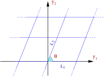
Figure 1: 2D torus characterized by the moduli $\theta$, $L_{1}$ and $L_{2}$, defined by the two identifications $(y_{1},y_{2})=(y_{1}+L_{1},y_{2})$ and $(y_{1},y_{2})=(y_{1}+L_{2}\cos\theta,y_{2}+L_{2}\sin\theta)$.

2.1 Scalar Field Casimir Energy

Consider a complex 6D field $\Phi$ on a space-time compactified to 4 dimensions on the above 2-torus. Writing the six coordinates as $\{x_{\mu},y_{i}\}$, with $\mu=0,...,3$ and $i=1,2$, assume the scalar satisfies the following boundary conditions

$$\Phi(x,y_{1}+n_{2}L_{2}\cos\theta+n_{1}L_{1};y_{2}+n_{2}L_{2}\sin\theta)=e^{2\pi i(n_{1}\,\rho_{1}+n_{2}\,\rho_{2})}\,\Phi(x,y_{1},y_{2})\,,$$ (3)

with $\rho_{1,2}$ being two real quantities. The choices $\rho_{1,2}=0,\frac{1}{2}$ correspond to periodic or anti-periodic boundary conditions along the torus’ two cycles. More general values of $\rho_{i}$ are also possible, such as when $\Phi$ transforms non-trivially under a gauge group for which nonzero Wilson lines are turned on for the corresponding cycles. Here we consider $\rho_{1,2}$ arbitrary.

Expanding the scalar field in terms of eigenfunctions of the 2D Laplacian, $\Box_{2}=\partial_{1}^{2}+\partial_{2}^{2}$, according to

$$\Phi(x,y)=\sum_{n_{1},n_{2}}\phi_{n_{1},n_{2}}(x)\,f_{n_{1},n_{2}}(y_{1},y_{2};\rho_{1},\rho_{2})\,,$$ (4)

we have $\Box_{2}f_{n_{1},n_{2}}=-M_{n_{1},n_{2}}^{2}\,f_{n_{1},n_{2}}$ with

$$M^{2}_{n_{1},n_{2}}(\rho_{1},\rho_{2}) = \frac{(2\pi)^{2}}{{\cal A}\,U_{2}}\,|n_{2}+\rho_{2}-U(n_{1}+\rho_{1})|^{2}\,.$$ (5)

Here ${\cal A}\!=\!L_{1}L_{2}\sin\theta$ denotes the area of the torus. The mode functions are given by

$$f_{n_{1},n_{2}}(y_{1},y_{2};\rho_{1},\rho_{2})=\frac{1}{\sqrt{\cal A}}\,e^{2i\,\pi[(n_{1}+\rho_{1})(y_{1}-y_{2}\cot\theta)/L_{1}+(n_{2}+\rho_{2})y_{2}/(L_{2}\sin\theta)]}\,.$$ (6)

We now compute the vacuum energy for a complex scalar field having 6D mass $m$, compactified on ${\cal T}_{2}$ with the above boundary conditions. Denoting the vacuum-energy per unit 3-volume for such a scalar field by $V(\rho_{1},\rho_{2})$, we have

$$V(\rho_{1},\rho_{2}) \equiv \mu^{4-d}\!\!\sum_{n_{1,2}\in{\bf Z}}\int\!\frac{d^{d}p}{(2\pi)^{d}}\ln\bigg{[}\frac{p^{2}\!+\!M_{n_{1},n_{2}}^{2}\!+m^{2}}{\mu^{2}}\bigg{]}\!$$ (7)

$$= -\frac{\mu^{4}}{(2\pi)^{d}}\!\!\sum_{n_{1,2}\in{\bf Z}}\int_{0}^{\infty}\!\!\!\!\!\frac{dt}{t^{1+d/2}}e^{-\pi\,t\,\big{[}\,(M_{n_{1},n_{2}}^{2}+m^{2})/\mu^{2}\big{]}}$$

where we have continued the momentum integration to Euclidean signature, and we regulate the ultraviolet divergences which arise in the sum and integral using dimensional regularization, with the complex quantity $d=4-\epsilon$ ultimately being taken to 4. Here $\mu$ denotes the arbitrary mass scale which arises in dimensional regularization, and which drops out of all physical quantities.

A potential subtlety arises in the above expression for massless 6D fields ($m=0$) if both $\rho_{1}$ or $\rho_{2}$ are integers, because in this case there is a choice of integers $(n_{1},n_{2})$ for which $M_{n_{1},n_{2}}$ vanishes. In this case it is convenient to keep $m$ nonzero so that all manipulations remain well-defined, with $m$ taken to zero at the end of the calculation. In principle, one must be alive to the possibility of unexpected singularities appearing when $m$ tends to zero after renormalization, such as the familiar infrared mass singularities of Quantum Electrodynamics [24]. As usual, such infrared problems are less severe in higher dimensions and we shall see that there is no such obstruction to taking $m\to 0$ for our applications in 6 dimensions.

The calculation of the two infinite sums in (7) is tedious, and is given in detail in Appendices A and B — c.f. eqs.(A-1), (B-1), (B) to (B-18) — using the approach of [25]. In what follows we quote only the final results which are appropriate to the discussion at hand. The next three sections respectively concentrate on the ultraviolet-divergent part of the result, as well as the finite part in the cases where the 6D scalars are either massless ($m^{2}{\cal A}\to 0$) or very massive ($m^{2}{\cal A}\gg 1$).

2.1.1 Ultraviolet Divergences for 2-Tori

The ultraviolet divergent part of $V$ in (7) denoted $V_{\infty}$ is, with $\epsilon=4-d$ (see eqs. (B-1), (B) to (B-18))

$$V_{\infty}(\rho_{1},\rho_{2})=\frac{m^{6}\,{\cal A}}{192\pi^{3}\epsilon}$$ (8)

which is valid for arbitrary $m$. (Eq.(8) shows the importance of keeping a non-zero $m$ when discussing ultraviolet divergences in dimensional regularization (DR), since these can easily be missed if $m=0$.) This expression has several features on which we now remark (and which agree with the more general analysis of the ultraviolet divergences in 6D field theories compactified on Ricci-flat backgrounds given in a companion paper [22]).

$\bullet$ First, the divergent part depends on the moduli, $L_{1,2}$ and $\theta$, only through the toroidal area ${\cal A}=L_{1}L_{2}\sin\theta$, and is interpreted as being a renormalization of the 6D cosmological constant. Note also that the UV divergence vanishes if we take $\theta\rightarrow 0$, corresponding to collapsing the two cycles of the torus onto each other down to one dimension less. This agrees with the well-known absence of one-loop UV divergences for a broad class of theories when they are dimensionally regularized in odd dimensions.

$\bullet$ The proportionality to $m^{6}$ is also what is required on dimensional grounds (in dimensional regularization) for a contribution to the 6D cosmological constant. The absence of other powers of $m$, such as an ${\cal A}$-independent result proportional to $m^{4}$, is a consequence of the torus being flat, and is not true for more general curved spacetimes [22]. Once the UV divergence is renormalized into the 6D cosmological constant there is no obstruction to taking $m\to 0$, unlike the situation for massless 4D theories. We consequently feel free to simply set $m=0$ in subsequent applications of our formulae for $V^{\rm ren}$ where

$$V^{\rm ren}\equiv V-V_{\infty}$$ (9)

with $V$ as in (7) and $V_{\infty}$ its divergent part.

$\bullet$ The divergent part of $V$ is $\rho_{i}$-independent and so does not depend on the boundary conditions of the scalar field, eqs.(3). Again this agrees with general arguments, since the short-wavelength modes responsible for the UV properties are not sensitive to the boundary conditions which depend on the global properties of the background geometry. We shall see that for orbifolds new divergences are present corresponding to counterterms localized at the fixed points, and these new divergences can depend on the nature of the boundary conditions imposed on the covering space.

$\bullet$ The $1/\epsilon$ pole which appears here represents a bona fide 6D divergence. This is at first sight surprising, since $\epsilon$ represents the difference between $d$ and 4 rather than 6, and it is introduced for each of the Kaluza-Klein (KK) modes. To understand this it is important to recognize that our expressions contain two separate sources of UV divergence: the integration over 4-momentum, $p$, and the two sums over KK mode numbers, $n_{i}$. In our calculations the dimensional continuation is $\epsilon=4-d$ away from four in order to regularize the $p$-integration. On the other hand, the KK mode sums are managed using zeta-function techniques, and the presence of $\epsilon$ ensures the regularisation of these sums. With these choices the leading inverse powers of $\epsilon$ obtained turn out to be precisely those which would be obtained starting from 6D and following the powers of $\epsilon^{\prime}=(6-d)$. This equivalence is shown in more detail for an explicit example (using a spherical geometry, for which more divergences may be followed) in ref. [22].

We now examine the finite parts of the Casimir energy density.

2.1.2 Massless Fields in 6D

In the massless limit, $m\to 0$, the result for the vacuum energy density is (see eqs.(A-3), (B-1), (B) to (B-18))

$$V^{\rm ren}(\rho_{1},\rho_{2})|_{m=0}=-\frac{1}{{\cal A}^{2}}\,\left\{\,\frac{(2\pi U_{2})^{3}}{90}\,\left[\frac{1}{21}-\Delta_{\rho_{1}}^{2}\,\left(1-5\,\Delta_{\rho_{1}}^{2}-2\,\Delta_{\rho_{1}}^{4}+6\,\Delta_{\rho_{1}}^{3}\right)\right]\right.$$

$$\qquad+\sum_{n_{1}\in{\bf Z}}\left[(n_{1}+\Delta_{\rho_{1}})^{2}\,\mbox{Li}_{3}(\sigma_{n_{1}})+\frac{3\left|n_{1}+\Delta_{\rho_{1}}\right|}{2\pi U_{2}}\,\mbox{Li}_{4}(\sigma_{n_{1}})\right.\left.\left.+\frac{3}{(2\pi U_{2})^{2}}\,\mbox{Li}_{5}(\sigma_{n_{1}})+c.c.\right]\!\right\}$$

with

$$\sigma_{n_{1}\geq 0}=e^{-2i\,\pi\big{(}\Delta_{\rho_{2}}-U\Delta_{\rho_{1}}-Un_{1}\big{)}}\qquad\hbox{and}\qquad\sigma_{n_{1}<0}=\frac{1}{\overline{\sigma}_{n_{1}>0}}\,,$$ (10)

where $\overline{\sigma}_{n_{1}}$ denotes the complex conjugate of $\sigma_{n_{1}}$. In these expressions $0\leq\Delta_{\rho_{i}}<1$ represents the fractional part of $\rho_{i}$, as in $\rho_{i}=[\rho_{i}]+\Delta_{\rho_{i}}$, where $[\rho_{i}]\in{\bf Z}$ is the largest integer smaller than or equal to $\rho_{i}$. The poly-logarithm functions which appear here are defined by the sums [26]

$$\mbox{Li}_{\sigma}(x)=\sum_{n=1}^{\infty}\frac{x^{n}}{n^{\sigma}}\,.$$ (11)

The point of rewriting the initial two sums into the ones written here is that these converge well and so are useful for numerical purposes. Figure 2 plots $V(\rho_{1},\rho_{2})$ as functions of the moduli $U_{1}$ and $U_{2}$ for various choices for the boundary conditions $(\rho_{1},\rho_{2})$.

We have checked that the above formula agrees with the particular cases studied in the literature. For instance in the special case $\rho_{1}=\rho_{2}=0$ we find

$$V^{\rm ren}(0,0)\big{|}_{m=0} = -\frac{1}{{\cal A}^{2}}\,\bigg{\{}\frac{4\pi^{3}U_{2}^{3}}{945}+\frac{3\,\zeta[5]}{2\pi^{2}U_{2}^{2}}+2\sum_{n_{1}=1}^{\infty}\Big{[}n_{1}^{2}\,\mbox{Li}_{3}(q^{n_{1}})\phantom{\frac{1}{2}}$$ (12)

$$\qquad\qquad+\frac{3\,n_{1}}{2\pi U_{2}}\,\mbox{Li}_{4}(q^{n_{1}})+\frac{3}{4\pi^{2}U_{2}^{2}}\,\mbox{Li}_{5}(q^{n_{1}})+c.c.\Big{]}\bigg{\}},$$

where $q\equiv e^{2i\pi U}$. This agrees with the result given in ref. [6].

2.1.3 Heavy-Mass Dependence

The generality of the calculation in Appendix A, B also allows the explicit exhibition of the heavy-mass limit, $m^{2}{\cal A}\to\infty$, of the Casimir energy. This is of particular interest for Supersymmetric Large Extra Dimensions, where the naturalness of the description of the Dark Energy density relies on the Casimir energy only depending weakly on the masses of heavy fields in the 6D bulk. Using formulae (B), (B-16), (B-18) of the appendix it may be shown that if $m\gg\{1/L_{1},1/(L_{2}\sin\theta)\}$, leading to $m^{2}{\cal A}\gg 1$, then

$$V(\rho_{1},\rho_{2})=\frac{m^{6}\,{\cal A}}{384\pi^{3}}\Big{(}\frac{2}{\epsilon}-\ln\frac{4\pi^{3}m^{2}e^{\gamma-11/6}}{\mu^{2}}\Big{)}+\frac{1}{{\cal A}^{2}}\,{\cal O}\Big{(}(m^{2}{\cal A})^{\mu}\,U_{2}^{\nu}\,e^{-2\pi(m^{2}{\cal A})^{\sigma}U_{2}^{\pm\sigma}}\Big{)}$$ (13)

thus powers of $m^{2}{\cal A}$ other than $m^{6}$ are exponentially suppressed. These expressions agree well with the general results of ref. [22], which identify the large-$m$ behaviour using general heat-kernel techniques. For general geometries there can be powers of $m$ in the large-$m$ limit, but the leading such powers are proportional to local effective interactions which involve polynomials of the background fields and their derivatives. For the simple toroidal geometries considered here all of these local interactions vanish, leading to the exponential mass suppression found above.

The absence of powers like $m^{4}$ or $m^{2}$ in the large-$m$ limit is more difficult to understand from the point of view where the 6D calculation is regarded as simply being the sum over an infinite number of 4D contributions, each of which can themselves have such powers of $m$. As is clear from the general 6D analysis of [22], the absence of these terms may be traced to the requirements of locality and general covariance in 6 dimensions — requirements which are easily missed in a KK mode sum calculation.

2.2 Higher-Spin Fields on ${\cal T}_{2}$.

With an eye towards applications to supersymmetric theories, in this section we compute the corresponding results for the Casimir energy for other massless fields in 6 dimensions. We do so using the trick of ref. [6], which uses the prior knowledge that the Casimir energy must vanish once summed over the field content of a 6D supermultiplet, provided that these fields all share the same boundary conditions about the cycles of ${\cal T}_{2}$ (and so do not break any of the supersymmetries).

Multiplet	Field Content
Hyper	($\psi_{+}$, 2$\phi$)
Gauge	($A_{M}$, 2$\psi_{-}$)
Tensor	($A_{MN}^{+}$, 2$\psi_{+}$,$\phi$)
Gravitino I	($\psi_{M+}$, 2$A_{MN}^{-}$)
Gravitino II	($\psi_{M-}$, 2$A_{M}$,$\psi_{-}$)
Graviton	($g_{MN}$, 2$\psi_{M+}$, $A_{MN}^{-}$)

Table 1: The field content of some of the massless representations of $(2,0)$ supersymmetry in 6 dimensions. The fermions are taken to be symplectic-Weyl, and their plus and minus subscripts correspond to their chirality, as measured by their $\Gamma_{7}$ eigenvalue. The $+$ ($-$) sign on the 2-form potential similarly indicates it is self (anti-self) dual. There is also an equivalent set of representations where all plus and minus signs are interchanged.

To this end we reproduce as Table 1 a table from ref. [22] listing the massless field content of some of the representations of $(2,0)$ supersymmetry in 6 dimensions. In this table the scalars are real, the spinors are symplectic-Weyl and the 2-form gauge potentials are self-dual or anti-self-dual.

The argument of ref. [6] uses the observation that a single symplectic-Weyl fermion and two real scalars preserve 6-dimensional $(2,0)$ supersymmetry in a toroidal compactification for which they share the same boundary conditions, $(\rho_{1},\rho_{2})$, about the torus’ two cycles. The Casimir energy for these fields must therefore cancel in order to give a vanishing result for the contribution of a hypermultiplet. Since we know the scalar result for general $\rho_{i}$, we may infer from this that the Casimir energy for a single symplectic-Weyl fermion must be precisely $-1$ times the result quoted above for a complex scalar field having the same boundary conditions.

Using the identical argument based on the vanishing of the Casimir energy summed over the field content of a gauge multiplet similarly shows that the Casimir energy of a 6D gauge boson must be $-2$ times the result for a 6D symplectic-Weyl fermion — and so is $+2$ times the result for a 6D complex scalar — having the same boundary conditions. Arguing in this way allows the inference of the Casimir energy for all of the other fields appearing in the supermultiplets listed in Table 1. The results found in this way are

$$V_{1/2}(\rho_{1},\rho_{2}) = -V(\rho_{1},\rho_{2})$$

$$V_{1}(\rho_{1},\rho_{2}) = 2\,V(\rho_{1},\rho_{2})$$

$$V_{KR}(\rho_{1},\rho_{2}) = \frac{3}{2}\,V(\rho_{1},\rho_{2})$$

$$V_{3/2}(\rho_{1},\rho_{2}) = -3\,V(\rho_{1},\rho_{2})$$

$$V_{2}(\rho_{1},\rho_{2}) = -V(\rho_{1},\rho_{2})\,,$$ (14)

where the divergent and finite parts of the right-hand side of this equation are given explicitly by eqs. (8) and (2.1.2), above. Here $V_{1/2}$, $V_{1}$, $V_{KR}$, $V_{3/2}$ and $V_{2}$ respectively denote the results for a symplectic-Weyl fermion, a gauge boson, a Kalb-Ramond self-dual (or anti-self-dual) 2-form gauge potential, a symplectic-Weyl gravitino and a graviton.

Given these expressions, it is simple to compute the nonzero Casimir energy which results when 6D supersymmetry is broken à la Scherk and Schwarz [27], by assigning different boundary conditions to different fields within a single supermultiplet. Supersymmetry is broken in this case by the boundary conditions themselves. For instance, if the symplectic-Weyl fermion in a hypermultiplet has boundary condition $(\rho_{1},\rho_{2})$ but the complex scalar has boundary condition $(\rho^{\prime}_{1},\rho^{\prime}_{2})$ then the Casimir energy for this hypermultiplet would be

$$V_{\rm hyper}=V_{1/2}(\rho_{1},\rho_{2})+V(\rho^{\prime}_{1},\rho^{\prime}_{2})=V(\rho^{\prime}_{1},\rho^{\prime}_{2})-V(\rho_{1},\rho_{2})\,.$$ (15)

Similarly applying different boundary conditions to the constituents of a gauge or tensor multiplet gives

$$V_{\rm gauge} = V_{1}(\rho_{1},\rho_{2})+2\,V_{1/2}(\rho^{\prime}_{1},\rho^{\prime}_{2})=2\,[V(\rho_{1},\rho_{2})-V(\rho^{\prime}_{1},\rho^{\prime}_{2})]$$

$$V_{\rm tensor} = V_{KR}(\rho_{1},\rho_{2})+2\,V_{1/2}(\rho^{\prime}_{1},\rho^{\prime}_{2})+\frac{1}{2}\,V(\rho^{\prime\prime}_{1},\rho^{\prime\prime}_{2})$$ (16)

$$= \frac{3}{2}\,V(\rho_{1},\rho_{2})-2\,V(\rho^{\prime}_{1},\rho^{\prime}_{2})+\frac{1}{2}\,V(\rho^{\prime\prime}_{1},\rho^{\prime\prime}_{2})\,,$$

and so on.

Figure 2 gives in addition to the plots of $V(\rho_{1},\rho_{2})$, the differences $V(\rho_{1},\rho_{2})-V(\rho^{\prime}_{1},\rho^{\prime}_{2})$ as functions of $U_{1}$ and $U_{2}$ for various choices for the boundary conditions $(\rho_{1},\rho_{2})$ and $(\rho^{\prime}_{1},\rho^{\prime}_{2})$. The periodicity wrt $U_{1}$ in the plots is a remnant of the $SL(2,Z)_{U}$ symmetry (modified by non-zero Wilson lines). For $U_{2}=L_{2}/L_{1}\sin\theta\geq{\cal O}(1)$, one has flat directions for $V$ (as function of $U_{1},U_{2}$). This changes for $U_{2}\ll 1$ (say if $\theta\ll 1$) when $V$ develops maxima/minima. For values of $\rho_{i}$ other than those in the figure, the peaks in these plots have different height.

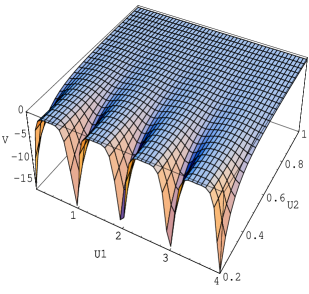
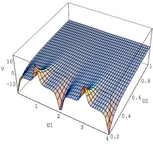
(a) The potential $V^{ren}$ for $\rho_{1}=\!\rho_{2}=0$.    (b) The potential $V^{ren}$ for $\rho_{1}=\!1/2,\,\rho_{2}\!=0$.

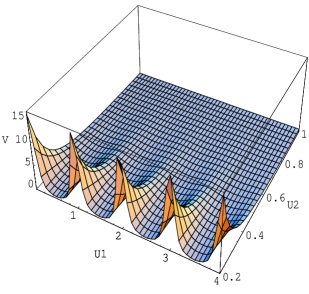
   (c) The potential $V^{ren}$ for $\rho_{1}=0,\rho_{2}=1/2$.
   (d) The potential $V^{ren}$ for $\rho_{1}\!=\!1/2,\rho_{2}\!=\!1/2$.
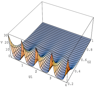
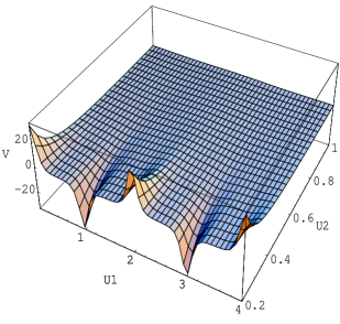
   (e) The plot $V^{ren}\big{|}_{\rho_{1}\!=\!0,\,\rho_{2}\!=\!\frac{1}{2}}-V^{ren}\big{|}_{\rho_{1}=\!\rho_{2}\!=\!0}$    (f) The plot $V^{ren}\big{|}_{\rho_{1}\!=\!\rho_{2}\!=\!\frac{1}{2}}-V^{ren}\big{|}_{\rho_{1}=\frac{1}{2},\,\rho_{2}=0}$

Figure 2: The (finite part of the) potential $V$, up to an overall positive factor and for fixed area ${\cal A}$. The plots are in function of $U_{1}$, $U_{2}$, ($U\!\equiv\!U_{1}\!+\!iU_{2}\!=\!L_{2}/L_{1}\exp(i\theta)$) for various $\rho_{1,2}$. See also eqs.(2.1.2) and (3.1.2). The peaks of the plots indicate (moduli) divergences present at $U_{2}\ll 1$ when the two dimensions collapse onto each other ($\theta=0$).

3 Casimir Energy for Orbifolds

None of the previous results included the effects of 3-branes within the bulk when computing the Casimir energies. We now extend these calculations to some simple examples which include branes, and for which the background geometry includes the back-reaction of the brane tensions by incorporating the appropriate conical singularities at the brane positions. We only consider here brane singularities which correspond to the specific defect angles which arise when an orbifold is constructed from the 2-torus by identifying points under the action, $Z_{N}$, of a discrete set of rotations. We analyze separately the case of ${\cal T}_{2}/Z_{2}$, with full details, and then the orbifold ${\cal T}_{2}/Z_{4}$ whose technical details differ considerably. For ${\cal T}_{2}/Z_{4}$ we use a general method which can be applied to the remaining ${\cal T}_{2}/Z_{3}$ and ${\cal T}_{2}/Z_{6}$.

To this end we return to the description of ${\cal T}_{2}$ as a complex plane, $z=y_{1}+i\,y_{2}$, identified under the action of a lattice of discrete translations as in eq. (2). Following standard practice, we construct an orbifold from this torus by further identifying points under the action of the $Z_{N}$ rotations defined by

$$z\cong\tau^{k}\,z\,,$$ (17)

where $\tau=e^{2\pi i/N}$. This gives a well-defined coset space, ${\cal O}={\cal T}_{2}/Z_{N}$, provided that these rotations take the initial lattice which defines the torus onto itself. Notice that if $N=2$, then the rotation $z\cong-z$ is automatically a symmetry of the lattice for any value of the moduli $L_{1}$, $L_{2}$ and $\theta$, and so these three quantities are also moduli of the resulting orbifold, ${\cal O}$. On the other hand, if $N>2$ then the rotation is a symmetry of the lattice only for specific choices for the complex structure: $U\equiv(L_{2}/L_{1})e^{i\theta}=\tau$, and so $L_{2}=L_{1}=L$ and $\theta=2\pi/N$, and so only one modulus, $L$, in this case survives.

The coset ${\cal T}_{2}/Z_{N}$ is an orbifold rather than a manifold because of the metric singularities which arise at the fixed points of the group. For instance, in the case ${\cal T}_{2}/Z_{2}$ there are 4 such points, corresponding to $z=0,\frac{1}{2},\frac{1}{2}\,U$ and $\frac{1}{2}(1+U)$. The metric has a conical singularity at each of these points, whose defect angle is $\pi$. For further details on orbifolds and their fixed points see Appendix D.

3.1 A Scalar Field on ${\cal T}_{2}/Z_{2}$.

We now compute the Casimir energy for a complex scalar field, $\Phi$, compactified from 6D to 4D on the orbifold ${\cal O}={\cal T}_{2}/Z_{2}$. As before, the 6 coordinates are taken to be $\{x,y_{i}\}$, with the orbifold corresponding to the coordinates $y_{i},i=1,2$. We consider the 6D scalar field to satisfy the boundary conditions

$$\Phi(x,y_{1}+L_{1};y_{2}) = e^{2\pi i\rho_{1}}\,\,\Phi(x,y_{1},y_{2});\qquad\rho_{1}=0,1/2.$$ (18)

$$\Phi(x,y_{1}+L_{2}\cos\theta;y_{2}+L_{2}\sin\theta) = e^{2\pi i\rho_{2}}\,\,\Phi(x,y_{1},y_{2});\qquad\rho_{2}=0,1/2.$$ (19)

$$\Phi(x,-y_{1},-y_{2}) = \pm\,\,\Phi(x,y_{1},y_{2})\,.$$ (20)

Condition (20) is possible because of the new cycle that the orbifold has (which the torus does not). As is indicated in eqs. (18) and (19), the quantities $\rho_{i}$ are no longer free to take any real value in this case, because the underlying Wilson lines must be compatible with the orbifold rotation. For instance, when acting on the coordinates it is straightforward to show that the composite transformation $X=\Sigma\circ P\circ\Sigma$ gives $X(y_{1},y_{2})=(-y_{1},-y_{2})$, if $\Sigma(y_{1},y_{2})=(y_{1}+L_{1},y_{2})$ and $P(y_{1},y_{2})=(-y_{1},-y_{2})$. Applying the same transformations to $\Phi$ and using the boundary conditions (18) and (20), consistency requires $\exp(4\pi i\rho_{1})=1$, and so $\rho_{1}=n/2$ for some integer $n$. A similar argument implies that $\rho_{2}$ is also half-integer. If we require, without loss of generality, $0\leq\rho_{i}<1$, then we see that consistency requires $\rho_{1,2}=0,1/2$. Altogether there are 8 possible choices for the boundary conditions, denoted by $(\rho_{1},\rho_{2})^{\pm}$.

Because the orbifold reflection is a symmetry of $\Box_{2}$, these reflections have a natural action on its eigenfunctions, $f_{n_{1},n_{2}}$. Using the explicit expressions obtained earlier, eq. (6), for the toroidal mode functions

$$f_{n_{1},n_{2}}(-y_{1},-y_{2};\rho_{1},\rho_{2}) = \frac{1}{\sqrt{\cal A}}\,e^{-2i\,\pi[(n_{1}+\rho_{1})(y_{1}-y_{2}\cot\theta)/L_{1}+(n_{2}+\rho_{2})y_{2}/(L_{2}\sin\theta)]}$$ (21)

$$= f_{n_{1},n_{2}}^{*}(y_{1},y_{2};\rho_{1},\rho_{2})\,,$$

$$\equiv f_{n_{1}^{\prime},n_{2}^{\prime}}(y_{1},y_{2};\rho_{1},\rho_{2})\,,$$

where $n^{\prime}_{i}=-n_{i}-2\rho_{i}$ ensures $n^{\prime}_{i}+\rho_{i}=-(n_{i}+\rho_{i})$. Notice that $n^{\prime}_{i}$ defined in this way remains an integer because for the $Z_{2}$ orbifold $\rho_{i}=0,\frac{1}{2}$.

Using this action it is straightforward to specialize the toroidal mode expansion, eq. (4), to fields on ${\cal T}_{2}/Z_{2}$ with boundary conditions $(\rho_{1},\rho_{2})^{\pm}$. We now write these expansions explicitly, in terms of the real and imaginary parts of the mode functions $f_{n_{1},n_{2}}=e_{n_{1},n_{2}}+ig_{n_{1},n_{2}}$.

(1). $(\rho_{1},\rho_{2})=(0,0)^{\pm}$. In this case $f_{n_{1},n_{2}}(-y_{1},-y_{2})=f_{-n_{1},-n_{2}}(y_{1},y_{2})$ and so using the boundary conditions of eqs. (20) in the mode expansion of eq. (4) gives

$$\Phi^{+}(x,y_{1},y_{2}) = \sum_{n_{1}\geq 0,\,n_{2}\in{\bf Z}}\frac{2}{2^{\delta_{n_{1},0}}}\,\phi_{n_{1},n_{2}}(x)\,\,e_{n_{1},n_{2}}(y_{1},y_{2};0,0),$$

$$\Phi^{-}(x,y_{1},y_{2}) = \sum_{n_{1}\geq 0,\,n_{2}\in{\bf Z}}^{\prime}\frac{2i}{2^{\delta_{n_{1},0}}}\,\phi_{n_{1},n_{2}}(x)\,\,g_{n_{1},n_{2}}(y_{1},y_{2};0,0),$$ (22)

where the superscript on $\Phi$ indicates the sign chosen for the orbifold projection, and $\delta_{n_{1},0}$ is the usual Kronecker delta-function which vanishes unless $n_{1}=0$, in which case it equals unity. Notice that because $g_{0,0}(y_{1},y_{2};0,0)=0$, the mode $(n_{1},n_{2})=(0,0)$ is absent in the double sum for $\Phi^{-}$, as is indicated by the primed double sum.

(2). $(\rho_{1},\rho_{2})=(0,1/2)^{\pm}$. In this case $f_{n_{1},n_{2}}(-y_{1},-y_{2})=f_{-n_{1},-n_{2}-1}(y_{1},y_{2})$ and so the mode expansion becomes

$$\Phi^{+}(x,y_{1},y_{2}) = \sum_{n_{1}\geq 0,\,n_{2}\in{\bf Z}}\frac{2}{2^{\delta_{n_{1},0}}}\,\phi_{n_{1},n_{2}}(x)\,\,e_{n_{1},n_{2}}(y_{1},y_{2};0,1/2),$$

$$\Phi^{-}(x,y_{1},y_{2}) = \sum_{n_{1}\geq 0,\,n_{2}\in{\bf Z}}\frac{2i}{2^{\delta_{n_{1},0}}}\,\phi_{n_{1},n_{2}}(x)\,\,g_{n_{1},n_{2}}(y_{1},y_{2};0,1/2).$$ (23)

(3). $(\rho_{1},\rho_{2})=(1/2,0)^{\pm}$. Here $f_{n_{1},n_{2}}(-y_{1},-y_{2})=f_{-n_{1}-1,-n_{2}}(y_{1},y_{2})$, and so

$$\Phi^{+}(x,y_{1},y_{2}) = \sum_{n_{1}\geq 0,\,n_{2}\in{\bf Z}}2\,\,\phi_{n_{1},n_{2}}(x)\,\,e_{n_{1},n_{2}}(y_{1},y_{2};1/2,0),\qquad$$

$$\Phi^{-}(x,y_{1},y_{2}) = \sum_{n_{1}\geq 0,\,n_{2}\in{\bf Z}}2i\,\phi_{n_{1},n_{2}}(x)\,\,g_{n_{1},n_{2}}(y_{1},y_{2};1/2,0),\qquad$$ (24)

(4). $(\rho_{1},\rho_{2})=(1/2,1/2)^{\pm}$. In this case $f_{n_{1},n_{2}}(-y_{1},-y_{2})=f_{-n_{1}-1,-n_{2}-1}(y_{1},y_{2})$, and so

$$\Phi^{+}(x,y_{1},y_{2}) = \sum_{n_{1}\geq 0,\,n_{2}\in{\bf Z}}2\,\,\phi_{n_{1},n_{2}}(x)\,\,e_{n_{1},n_{2}}(y_{1},y_{2};1/2,1/2),\,\,$$

$$\Phi^{-}(x,y_{1},y_{2}) = \sum_{n_{1}\geq 0,\,n_{2}\in{\bf Z}}2i\,\phi_{n_{1},n_{2}}(x)\,\,g_{n_{1},n_{2}}(y_{1},y_{2};1/2,1/2).\,\,$$ (25)

There are two ways to compute the Casimir energy for the scalar field $\Phi$ on ${\cal T}_{2}/Z_{2}$ with these boundary conditions. One approach is to recognize that the scalar propagator on the orbifold may be obtained from the propagator on the torus using the method of images:

$$G^{\pm}_{{\cal O}}(x-x^{\prime},y-y^{\prime})=G_{{\cal T}}(x-x^{\prime},y-y^{\prime})\pm G_{{\cal T}}(x-x^{\prime},y+y^{\prime})\,,$$ (26)

and following the implications of this for the vacuum energy. The second approach is to directly perform the KK mode sum over the modified mode functions given above. Both lead to the same result, and we present the mode-function derivation here because, albeit more involved, it can be extended to the case of ${\cal T}_{2}/Z_{N}$ and allows a general discussion of the ultraviolet divergences for ${\cal T}_{2}/Z_{N}$.

The vacuum energy density per unit 3-volume written as a mode sum is given by

$$V_{\cal O}(0,0)^{\pm} = \sum_{n_{1}\geq 0,\,n_{2}\in{\bf Z}}^{(-)^{\prime}}\frac{\mu^{4-d}}{2^{\delta_{n_{1},0}}}\int\frac{d^{d}p}{(2\pi)^{d}}\,\ln\bigg{[}\frac{p^{2}+M_{n_{1},n_{2}}^{2}(0,0)+m^{2}}{\mu^{2}}\bigg{]}$$

$$V_{\cal O}(0,1/2)^{\pm} = \sum_{n_{1}\geq 0,\,n_{2}\in{\bf Z}}\frac{\mu^{4-d}}{2^{\delta_{n_{1},0}}}\int\frac{d^{d}p}{(2\pi)^{d}}\,\ln\bigg{[}\frac{p^{2}+M_{n_{1},n_{2}}^{2}(0,1/2)+m^{2}}{\mu^{2}}\bigg{]}$$

$$V_{\cal O}({1}/{2},0)^{\pm} = \sum_{n_{1}\geq 0,\,n_{2}\in{\bf Z}}\,\mu^{4-d}\,\int\frac{d^{d}p}{(2\pi)^{d}}\,\ln\bigg{[}\frac{p^{2}+M_{n_{1},n_{2}}^{2}(1/2,0)+m^{2}}{\mu^{2}}\bigg{]}$$

$$V_{\cal O}({1}/{2},{1}/{2})^{\pm} = \sum_{n_{1}\geq 0,\,n_{2}\in{\bf Z}}\,\mu^{4-d}\,\int\!\frac{d^{d}p}{(2\pi)^{d}}\,\ln\bigg{[}\frac{p^{2}+M_{n_{1},n_{2}}^{2}(1/2,1/2)+m^{2}}{\mu^{2}}\bigg{]},$$ (27)

where $d=(4-\epsilon)$ and the symbol $(-)^{\prime}$ on the sum in the first line indicates the exclusion from the sum of the single mode $(n_{1},n_{2})=(0,0)$, but only for the case of $(0,0)^{-}$ boundary conditions.

As might be expected from the approach based on the method of images, these expressions may be evaluated in terms of the corresponding quantities on the torus. To see this for the mode sums we denote the summands of these expressions by ${\cal W}(|n_{2}+\rho_{2}-U(n_{1}+\rho_{1})|^{2})$ in order to emphasize their dependence on mode numbers and moduli. It is then simple to use the invariance of ${\cal W}$ under changes in sign of $(n_{i}+\rho_{i})$ to prove the following identities:

$$\sum_{n_{1}\geq 0;\,n_{2}\in{\bf Z}}\frac{1}{2^{\delta_{n_{1},0}}}{\cal W}\Big{(}|n_{2}-Un_{1}|^{2}\Big{)} = \frac{1}{2}\sum_{n_{1},n_{2}\in{\bf Z}}{\cal W}\Big{(}|n_{2}-Un_{1}|^{2}\Big{)}$$

$$\sum_{n_{1}\geq 0;\,n_{2}\in{\bf Z}}\frac{1}{2^{\delta_{n_{1},0}}}{\cal W}\Big{(}|n_{2}+1/2-Un_{1}|^{2}\Big{)} = \frac{1}{2}\sum_{n_{1},n_{2}\in{\bf Z}}{\cal W}\Big{(}|n_{2}+1/2-Un_{1}|^{2}\Big{)}$$

$$\sum_{n_{1}\geq 0;\,n_{2}\in{\bf Z}}{\cal W}\Big{(}|n_{2}+\rho_{2}-U(n_{1}+1/2)|^{2}\Big{)} = \frac{1}{2}\!\!\sum_{n_{1},n_{2}\in{\bf Z}}{\cal W}\Big{(}|n_{2}+\rho_{2}-U(n_{1}+1/2)|^{2}\Big{)},\quad$$ (28)

where $\rho_{2}$ is either 0 or $\frac{1}{2}$ in the last line. These expressions allow the derivation of the following expressions for the Casimir energies in terms of the toroidal results, $V(\rho_{1},\rho_{2})$

$$V_{\cal O}(0,0)^{-} = \frac{1}{2}\,\Bigl{[}V(0,0)-V_{\rm zm}\Bigr{]}$$

$$V_{\cal O}(\rho_{1},\rho_{2})^{\pm} = \frac{1}{2}\,V(\rho_{1},\rho_{2})\qquad\hbox{for all others.}$$ (29)

Here $V_{\rm zm}$ is the contribution to the torus Casimir energy of the “zero mode” $(n_{1},n_{2})\!=\!(0,0)$ with $(\rho_{1},\rho_{2})^{-}=(0,0)^{-}$ (for its expression see (B-17) and (B-18)). We can now present in detail the divergent and finite parts of the sums and integrals in (3.1), (3.1).

3.1.1 Ultraviolet Divergences

We isolate the divergent part of $V_{\cal O}$ in eqs.(3.1) and write

$$V_{\cal O}(\rho_{1},\rho_{2})^{\pm}=V_{{\cal O},\infty}(\rho_{1},\rho_{2})^{\pm}+V_{\cal O}^{\rm{ren}}(\rho_{1},\rho_{2})^{\pm}$$ (30)

where all divergent terms are included in $V_{{\cal O},\infty}$. As is clear from eqs. (3.1), for all choices of boundary condition except $(0,0)^{-}$ on the orbifold the ultraviolet divergences encountered are precisely half of those encountered on the torus, eq. (8):

$$V_{{\cal O}\infty}(\rho_{1},\rho_{2})^{\pm}=\frac{m^{6}\,{\cal A}}{384\pi^{3}\epsilon}=\frac{m^{6}\,{\cal A}_{\cal O}}{192\pi^{3}\epsilon}\,,\qquad\hbox{if}\qquad(\rho_{1},\rho_{2})^{\pm}\neq(0,0)^{-}\,.$$ (31)

This divergence may be absorbed, as usual, into a renormalization of the bulk cosmological constant. Notice that its coefficient is the same as was obtained earlier for the torus, once the divergence is expressed in terms of the area of the orbifold, ${\cal A}_{\cal O}$, which is half the area, ${\cal A}$, of the covering torus.

By contrast, the exclusion of the zero mode for the specific choice $(0,0)^{-}$ introduces a new type of divergence which was not encountered for the torus. In this case the orbifold and toroidal divergences differ by the contribution of the $n_{1}=n_{2}=0$ mode alone, and thus, using eqs.(A-3), (B-1), (B), (B), one has

$$V_{{\cal O}\infty}(0,0)^{-}=\frac{1}{2}\,V^{*}_{\infty}(0,0)=\frac{m^{6}\,{\cal A}_{\cal O}}{192\pi^{3}\epsilon}+\frac{m^{4}}{32\pi^{2}\epsilon}\,.$$ (32)

The presence of the last term is consistent with the general heat-kernel analysis. Because it is proportional to $m^{4}$ and is independent of the bulk moduli, it has the right properties to be interpreted as a renormalization of the tension of the branes whose presence at the fixed points is responsible for the conical singularities in the bulk geometry at these points. As before, the ultraviolet-finite part of the Casimir energy obtained after this renormalization is nonsingular in the $m\to 0$ limit, and so we are free to take this limit explicitly in the renormalized result for massless 6D fields which we quote below.

It should be emphasized that although this divergence renormalizes the local brane tensions, it arises due to the functional integration over bulk fields. This is a feature which arises quite generically for quantum effects in the presence of boundaries and defects, whose origin can be understood in detail as follows. The bulk vacuum energy density, $t_{MN}=\langle T_{MN}\rangle$ is ultraviolet finite (for the flat orbifold under discussion) after the bulk cosmological constant is appropriately renormalized. However although $t_{MN}$ is finite, it is also position-dependent due to the presence of the orbifold singularities breaking the translation invariance of the underlying torus. In particular, $t_{MN}(y)$ typically goes to infinity as the singular points are approached in a way which diverges once integrated over the volume of the orbifold. It is this new divergence which is renormalized by the brane-tension counter-term localized at the singularity.

3.1.2 6D Massless Fields

Using eqs.(3.1) we can now give the explicit results for the Casimir energy of a massless complex 6D scalar field compactified on ${\cal T}_{2}/Z_{2}$, for the various boundary conditions $(\rho_{1},\rho_{2})^{\pm}$. It is noteworthy that $V^{\rm ren}_{\rm zm}(0,0)$ vanishes as $m\to 0$ in dimensional regularization, and so the orbifold result is half of the appropriate toroidal result for all choices of boundary conditions. After the renormalization of the ultraviolet divergences described above, one has

$$V_{\cal O}^{\rm ren}(\rho_{1},\rho_{2})^{\pm}\big{|}_{m=0}=\frac{1}{2}V^{\rm ren}(\rho_{1},\rho_{2})\big{|}_{m=0},\qquad\rho_{1,2}=0,1/2.$$ (33)

and that

$$\quad V^{\rm ren}_{\cal O}(0,0)^{\pm}\Big{|}_{m=0}=-\frac{1}{{\cal A}^{2}}\,\bigg{\{}\bigg{(}\frac{1}{21}\bigg{)}\frac{(2\pi U_{2})^{3}}{180}+\frac{3\,\zeta[5]}{(2\pi U_{2})^{2}}$$

$$\hskip 89.626pt+\sum_{n_{1}=1}^{\infty}\Big{[}n_{1}^{2}\,\mbox{Li}_{3}(q^{n_{1}})+\frac{3\,n_{1}}{2\pi U_{2}}\,\mbox{Li}_{4}(q^{n_{1}})+\frac{3}{(2\pi U_{2})^{2}}\,\mbox{Li}_{5}(q^{n_{1}})+c.c.\Big{]}\bigg{\}}$$

$$V^{\rm ren}_{\cal O}(0,1/2)^{\pm}\Big{|}_{m=0}=-\frac{1}{{\cal A}^{2}}\,\bigg{\{}\bigg{(}\frac{1}{21}\bigg{)}\frac{(2\pi U_{2})^{3}}{180}-\frac{45\,\zeta[5]}{16(2\pi U_{2})^{2}}$$

$$\hskip 89.626pt+\sum_{n_{1}=1}^{\infty}\Big{[}n_{1}^{2}\,\mbox{Li}_{3}(-q^{n_{1}})+\frac{3\,n_{1}}{2\pi U_{2}}\,\mbox{Li}_{4}(-q^{n_{1}})+\frac{3}{(2\pi U_{2})^{2}}\,\mbox{Li}_{5}(-q^{n_{1}})+c.c.\Big{]}\bigg{\}}$$

$$V^{\rm ren}_{\cal O}({1}/{2},0)^{\pm}\Big{|}_{m=0}=-\frac{1}{{\cal A}^{2}}\,\bigg{\{}-\bigg{(}\frac{31}{672}\bigg{)}\frac{(2\pi U_{2})^{3}}{180}+\sum_{n_{1}=0}^{\infty}\Big{[}\big{(}n_{1}+1/2\big{)}^{2}\,\mbox{Li}_{3}\big{(}q^{n_{1}+{1}/{2}}\big{)}$$

$$\hskip 89.626pt+\,\frac{3\,\big{(}n_{1}+1/2\big{)}}{2\pi U_{2}}\,\mbox{Li}_{4}\big{(}q^{n_{1}+{1}/{2}}\big{)}+\frac{3}{(2\pi U_{2})^{2}}\,\mbox{Li}_{5}\big{(}q^{n_{1}+{1}/{2}}\big{)}+c.c.\Big{]}\bigg{\}}$$

$$V^{\rm ren}_{\cal O}({1}/{2},{1}/{2})\Big{|}_{m=0}=-\frac{1}{{\cal A}^{2}}\,\bigg{\{}-\bigg{(}\frac{31}{672}\bigg{)}\frac{(2\pi U_{2})^{3}}{180}+\sum_{n_{1}=0}^{\infty}\Big{[}\big{(}n_{1}+{1}/{2}\big{)}^{2}\,\mbox{Li}_{3}\big{(}-q^{n_{1}+{1}/{2}}\big{)}$$

$$\hskip 89.626pt+\,\frac{3\,\big{(}n_{1}+1/2\big{)}}{2\pi U_{2}}\mbox{Li}_{4}\big{(}-q^{n_{1}+{1}/{2}}\big{)}+\frac{3}{(2\pi U_{2})^{2}}\,\mbox{Li}_{5}\big{(}-q^{n_{1}+{1}/{2}}\big{)}\!+\!c.c.\Big{]}\!\!\bigg{\}}\qquad\,$$ (34)

where $q=e^{2\pi iU}$ and the complex conjugate applies only to the series of polylogarithms.

3.1.3 Heavy-Mass Dependence

The divergences of the Casimir energy for large $m$ are identical to those for the case of small $m$ discussed in Section 3.1.1. Further, because the orbifold results are simply expressed in terms of the toroidal ones, the heavy-mass dependence of the toroidal expressions carry over immediately to the orbifold Casimir energy. In particular, in dimensional regularization (and after modified minimal subtraction) the finite parts of the Casimir energy fall exponentially for large $m$, and the only strong $m$-dependence arises in the divergent terms, including the new $m^{4}$ term which arises for some of the boundary conditions.

3.1.4 Higher-Spin Fields on ${\cal T}_{2}/Z_{2}$

The results for massless higher-spin fields on the ${\cal T}_{2}/Z_{2}$ orbifold can be read from their toroidal counterparts of Section 2.2. This is possible because the orbifold identification does not break supersymmetry provided that all of the fields within a 6D supermultiplet satisfy the same boundary conditions. The results for the Casimir energy of higher-spin fields may therefore simply be read off by multiplying the expressions (3.1.2) by the factors given in eqs. (2.2).

3.2 The Orbifold ${\cal T}_{2}/Z_{N}$ with $N>2$.

In this section we outline the steps for computing the Casimir energy for a complex scalar field $\Phi$ compactified on the ${\cal T}_{2}/Z_{N}$ orbifolds, with $N>2$. Recall that for these orbifolds

$$U=e^{2i\pi/N},\qquad L_{2}=L_{1}=L,\qquad\theta=2\pi/N$$ (35)

We take the following action of the translation and orbifold $Z_{N}$ symmetries on the field $\Phi$

$$\Phi^{g}(x,\tau^{k}\,z) = g^{k}\,\Phi^{g}(x,z),$$

$$\Phi^{g}(x,z+L_{1}) = e^{2i\pi\rho_{1}}\,\Phi^{g}(x,z)$$

$$\Phi^{g}(x,z+UL_{1}) = e^{2i\pi\rho_{2}}\,\Phi^{g}(x,z)\,,$$ (36)

where we use complex coordinates $z=y_{1}+iy_{2}$ and as before $\tau\equiv e^{2i\pi/N}$ and $k=\overline{0,N-1}$. Here $g$ is a particular representation of the $Z_{N}$ transformation, acting on $\Phi^{g}$. The superscript ‘$g$’ emphasizes that this representation is not unique, and the explicit form taken by $\Phi^{g}$ in general depends on which $g$ is chosen. As in the case of ${\cal T}_{2}/Z_{2}$, this realization only faithfully reproduces the symmetry for specific choices for the $\rho_{i}$, whose values we now determine.

The consistency conditions for the action on $\Phi^{g}$ are found by combining the above expressions and using geometrical relations which state how some of the $Z_{N}$ rotations can also be expressed as translations on the covering torus. To display these we use the complex coordinate $z=y_{1}+iy_{2}$, in terms of which the lattice of translations which defines the underlying torus is generated by $e_{1}=L_{1}$ and $e_{2}=UL_{1}$. Then, depending on the group of rotations, $Z_{N}$, which is of interest, the following restrictions can arise.

• If an orbifold rotation takes $e_{1}$ to $e_{2}$ — i.e. there is an integer $0<k<N$ for which $\tau^{k}e_{1}=e_{2}$ (or $\tau^{k}=U$) — then using eqs. (3.2) to evaluate $\Phi^{g}(x,\tau^{k}(z+e_{1}))=\Phi^{g}(x,\tau^{k}z+e_{2}\big{)}$ implies

  $$g^{k}\,\exp(2\pi i\rho_{1})=g^{k}\,\exp(2\pi i\rho_{2})\,,$$ (37)

  and so we may take $\rho_{1}=\rho_{2}$ without loss of generality.

• If an orbifold rotation takes $e_{i}\to-e_{i}$ then a similar argument implies

  $$g^{k}\,\exp(2\pi i\rho_{i})=g^{k}\,\exp(-2\pi i\rho_{i})\,,$$ (38)

  and so we may take $\rho_{i}=0$ or $1/2$.

For instance, only the second of these conditions applied to the $Z_{2}$ orbifold considered previously. By contrast, both conditions apply to the case of $\pi/N$ rotations which give the orbifold ${\cal T}_{2}/Z_{2N}$, and so for this case we must take $\rho_{1}=\rho_{2}=0,\frac{1}{2}$. For the $Z_{3}$ case, on the other hand, the first condition applies but instead of the second condition one has $e_{2}+\tau^{k}e_{2}=-e_{1}$, and so we find $\rho_{2}=\rho_{1}=0,\frac{1}{3}$ or $\frac{2}{3}$. These results express the quantization on these orbifolds of the underlying Wilson lines which are responsible for the boundary conditions which are expressed by the $\rho_{i}$. For a more detailed description of Wilson lines and their values on orbifolds see Appendix D.

To determine the action of the symmetries (3.2) on the toroidal mode functions, we adapt the discussion of Section 2.3 of ref. [28] to include the general phases $\rho_{1,2}$. It is convenient for these purposes to rewrite eq. (6) in complex coordinates

$$f_{{\underline{n}}_{1},{\underline{n}}_{2}}(z,\bar{z})=\frac{1}{\sqrt{\cal A}}\,\,e^{[({\underline{n}}_{2}-{\underline{n}}_{1}{\overline{U}})\,z\,-\,({\underline{n}}_{2}-{\underline{n}}_{1}U)\,{\overline{z}}]/(2L_{1}U_{2})},$$ (39)

where ${\underline{n}}_{i}=n_{i}+\rho_{i}$, for $i=1,2$. The construction of the mode functions for the orbifold ${\cal T}_{2}/Z_{N}$ is done by observing that all of the arguments in [28] remain valid if $n_{i}$ is replaced by ${\underline{n}}_{i}=n_{i}+\rho_{i}$. The basis functions one is led to are given by

$$h^{g}_{\underline{n}_{1},{\underline{n}}_{2}}(z)=\frac{1}{\sqrt{N}}\,\,\eta_{{\underline{n}},{\underline{0}}}\sum_{k=0}^{N-1}g^{-k}f_{\underline{n}_{1},{\underline{n}}_{2}}(\tau^{k}\,z)$$ (40)

where $\eta_{{\underline{n}},{\underline{0}}}=1/{\sqrt{N}}$ if ${\underline{n}}_{1}={\underline{n}}_{2}=0$, and otherwise equals 1. Using this definition, one can check that the mode functions satisfy the orbifold condition

$$h^{g}_{\underline{n}_{1},{\underline{n}}_{2}}(\tau^{k}z)=g^{k}\,h^{g}_{\underline{n}_{1},{\underline{n}}_{2}}(z)\,.$$ (41)

As outlined in [28] not all the functions $h_{{\underline{n}}_{1}{\underline{n}}_{2}}$ are independent, since they are related by

$$h_{\omega^{k}(\tau)\cdot({\underline{n}}_{1},{\underline{n}}_{2})}^{g}(z)=h^{g}_{{\underline{n}}_{1},{\underline{n}}_{2}}(\tau^{k}\,z),$$ (42)

where $\omega^{k}(\tau)\cdot({\underline{n}}_{1},{\underline{n}}_{2})$ is defined as a rotation which takes $-{\underline{n}}_{1}+\tau{\underline{n}}_{2}$ into $-{\underline{n}}_{1}^{\prime}+\tau{\underline{n}}_{2}^{\prime}=\tau^{k}(-{\underline{n}}_{1}+\tau{\underline{n}}_{2})$. The set of all such rotations (i.e. for $k=0,1,..,N-1$) identify $N$ domains whose union covers the whole complex plane $(Ox;Oy)$ defined by $(Ox;Oy)=(-{\underline{n}}_{1}+\tau_{1}{\underline{n}}_{2};\tau_{2}{\underline{n}}_{2})$. Each such domain fixes the set of levels ${\underline{n}}_{1},{\underline{n}}_{2}$ which identify the set of independent $h_{{\underline{n}}_{1},{\underline{n}}_{2}}^{g}$ which are not related by the rotation $\omega$ of (42). This gives ${\underline{n}}_{1}\!=\!n_{1}\!+\!\rho_{1}\!<\!0$ and ${\underline{n}}_{2}\!=\!n_{2}\!+\!\rho_{2}\geq 0$ as an independent set. Since here $0\!\leq\!\rho_{1,2}\!<\!1$, one concludes that the conditions $n_{1}\!<\!0,n_{2}\!\geq\!0$ define an independent set of functions $h_{{\underline{n}}_{1},{\underline{n}}_{2}}$ for the orbifold ${\cal T}_{2}/Z_{N}$.

Using the above considerations, one has the following mode decomposition for $\Phi^{g}$:

$$\Phi^{g}(x,z)=\sum_{n_{1}<0,n_{2}\geq 0}\Phi^{g}_{\underline{n}_{1},{\underline{n}}_{2}}(x)\,\,h_{\underline{n}_{1},{\underline{n}}_{2}}(z)+\frac{\delta^{g,1}}{\sqrt{\cal A}}\,\,\Phi^{1}_{\underline{0},\underline{0}},\qquad{\underline{n}}_{i}=n_{i}+\rho_{i}\,,$$ (43)

which satisfies the desired condition $\Phi^{g}(x,\tau^{k}z)\!=\!g^{k}\,\Phi^{g}(x,z)$. For example, for ${\cal T}_{2}/Z_{3}$

$$g=\tau^{0},\qquad\Phi^{0}(x,z) = \sum_{n_{1}<0,n_{2}\geq 0}\phi^{0}_{{\underline{n}}_{1},{\underline{n}}_{2}}(x)\,\,\bigg{[}\frac{1}{\sqrt{3}}\sum_{k=0}^{2}f_{{\underline{n}}_{1},{\underline{n}}_{2}}(\tau^{k}\,z)\bigg{]}+\frac{1}{\sqrt{\cal A}}\phi^{0}_{{\underline{0}},{\underline{0}}}(x)$$

$$g=\tau^{1},\qquad\Phi^{1}(x,z) = \sum_{n_{1}<0,n_{2}\geq 0}\phi^{1}_{{\underline{n}}_{1},{\underline{n}}_{2}}(x)\,\,\bigg{[}\frac{1}{\sqrt{3}}\sum_{k=0}^{2}\tau^{-k}\,f_{{\underline{n}}_{1},{\underline{n}}_{2}}(\tau^{k}\,z)\bigg{]}$$

$$g=\tau^{2},\qquad\Phi^{2}(x,z) = \sum_{n_{1}<0,n_{2}\geq 0}\phi^{2}_{{\underline{n}}_{1},{\underline{n}}_{2}}(x)\,\,\bigg{[}\frac{1}{\sqrt{3}}\sum_{k=0}^{2}\tau^{-2k}\,f_{{\underline{n}}_{1},{\underline{n}}_{2}}(\tau^{k}\,z)\bigg{]}$$ (44)

The main difference from the ${\cal T}_{2}/Z_{2}$ orbifold is that for ${\cal T}_{2}/Z_{N}$ the sum over the Kaluza-Klein levels is restricted to positive/negative values of $n_{1,2}$, unlike in ${\cal T}_{2}/Z_{2}$ where one sum could be extended to the whole set ${\bf Z}$ of integers. The above mode expansion leads to the following expression for the Casimir energy of a complex 6D scalar field on ${\cal T}_{2}/Z_{N}$, $N\!>\!2$.

$$V_{\cal O}\left(\rho_{1},\rho_{2}\right) = \sum_{n_{1}<0,\,n_{2}\geq 0}\mu^{4-d}\int\frac{d^{d}p}{(2\pi)^{d}}\ln\bigg{[}\frac{p^{2}+M_{n_{1},n_{2}}^{2}(\rho_{1},\rho_{2})+m^{2}}{\mu^{2}}\bigg{]}\,$$ (45)

where for each $g$ one uses the values of $\rho_{1,2}$ which respect the consistency conditions.

The above domain of summation for $n_{1,2}$ makes the analytical calculation of $V_{\cal O}(\rho_{1},\rho_{2})$ more difficult than in the case of ${\cal T}_{2}/Z_{2}$. The difficulty is caused by the fact that none of the sums over $n_{1}$, $n_{2}$ can be extended to a sum over the whole set ${\bf Z}$ of integers (as we had for ${\cal T}_{2}/Z_{2}$, eq.(3.1)). As a result no (Poisson) resummation of individual contributions to $V(\rho_{1},\rho_{2})$ is possible and the calculation is then more tedious. Although one may still be able to work on the covering torus rather than in the orbifold basis, the approach below (being valid for any $\rho_{1,2}$) allows a simultaneous analysis of all orbifolds ${\cal T}_{2}/Z_{N}$, $N\!>\!2$.

After a long calculation (see Appendix C, eqs.(C-1) to (C-9)) one has for $V(\rho_{1},\rho_{2})$ of (45) the following result (which is valid for $m\ll 1/L$)

$$V_{\cal O}(\rho_{1},\rho_{2}) = -\frac{1}{2\,{\cal A}^{2}}\,\bigg{\{}\tilde{\cal D}+\frac{m^{6}{\cal A}^{3}}{768\,\pi^{3}}\frac{-2}{\epsilon}+\frac{(2\pi U_{2})^{3}}{180}\bigg{[}\frac{1}{21}\!-\rho_{1}^{2}(1-5\rho_{1}^{2}-\!2\rho_{1}^{4}+6\rho_{1}^{3})\bigg{]}\!$$

$$+ \!\!\!\!\!\sum_{n_{1}<0}\bigg{[}(n_{1}+\rho_{1})^{2}\,\mbox{Li}_{3}(\sigma_{n_{1}})\!+\!\frac{3\,|n_{1}+\rho_{1}|}{2\pi\,U_{2}}\,\mbox{Li}_{4}(\sigma_{n_{1}})\!+\!\frac{3}{4\pi^{2}U_{2}^{2}}\,\mbox{Li}_{5}(\sigma_{n_{1}})\!+\!c.c.\bigg{]}\!\bigg{\}}\qquad\,\,$$ (46)

where

$$\sigma_{n_{1}<0}=e^{-2i\pi\big{(}U(n_{1}+\rho_{1})-\rho_{2}\big{)}},\qquad 0\leq\rho_{i}<1,\qquad U=U_{1}+i\,U_{2},\,\,U_{2}>0.$$ (47)

This is the result for the Casimir energy for ${\cal T}_{2}/Z_{N}$, $N\!>\!2$ with boundary conditions as in (3.2) and with $\rho_{1,2}$ taking the values required by the consistency conditions specific to each orbifold. Finally, $\tilde{\cal D}$ of (3.2) is an asymptotic series given by (see Appendix C, eq.(C-10))

$$\tilde{\cal D}\!=\!\frac{(\mu^{2}{\cal A})^{\frac{\epsilon}{2}}}{\pi^{{\epsilon}/{2}-2}}\!\!\!\!\!\!\sum_{n_{1}<0,p\geq 0}\!\frac{2\,(-1)^{p}}{p!\,U_{2}^{2p-2}}\,\Gamma\Big{[}p-2+\frac{\epsilon}{2}\Big{]}\,\zeta\big{[}-2p,\rho_{2}-U_{1}(n_{1}+\rho_{1})\big{]}\,\Big{[}\frac{m^{2}{\cal A}}{(2\pi)^{2}U_{2}}+(n_{1}+\rho_{1})^{2}\Big{]}^{2-p-\frac{\epsilon}{2}}$$ (48)

where $\zeta[q,x]$ is the Hurwitz zeta function [26], ${\cal A}=L^{2}\sin\theta$, $U_{2}={\rm Im}U=\sin\theta$, $\theta=2\pi/N$. This expression of $\tilde{\cal D}$ is valid without any restrictions on the relative values of $m$, $L$ or $U$.

The quantity $\tilde{\cal D}$ is of particular interest because it contains additional poles as $\epsilon\to 0$, and so potentially introduces new contributions to the UV divergent part of $V_{\cal O}$ in (3.2). Note that if one of the sums (say that over $n_{2}\geq 0$) in $V_{\cal O}$ of (45) were extended to the whole ${\bf Z}$ set of integers, the quantity $\tilde{\cal D}$ given above would not arise due to the cancellation against the similar contribution to $V_{\cal O}$, coming from $n_{2}<0$. The latter would actually be equal to $\tilde{\cal D}$ of (48) with the substitutions $\rho_{2}\rightarrow 1-\rho_{2}$ and $U_{1}\rightarrow-U_{1}$. The sum of these two contributions would then vanish

$$\tilde{\cal D}(\rho_{1},\rho_{2})+\tilde{\cal D}(\rho_{1},1-\rho_{2})\Big{|}_{U_{1}\rightarrow-U_{1}}=0$$ (49)

since $\zeta[-2m,x]+\zeta[-2m,1-x]=0$. In particular, this explains the absence of $\tilde{\cal D}$ in ${\cal T}_{2}$ and ${\cal T}_{2}/Z_{2}$ where one of the KK sums was over the whole set ${\bf Z}$. To conclude, the presence of $\tilde{\cal D}$ in the potential $V_{\cal O}$ is due to the fact that both sums over the Kaluza-Klein modes in (45) were restricted to positive/negative modes only.

3.2.1 Ultraviolet Divergences

Because the contribution $\tilde{\cal D}$ potentially introduces new UV divergences for ${\cal T}_{2}/Z_{N}$ orbifolds with $N>2$, in this section we investigate their form in more detail in order to see what kinds of counterterms they require. In particular, we show that for ${\cal T}_{2}/Z_{2N}$ no new counterterms are required beyond those which already arise for the $Z_{2}$ orbifold. To do so we consider in detail the case of ${\cal T}_{2}/Z_{4}$, for which the analysis of $\tilde{\cal D}$ is considerably simplified. For the remaining cases ${\cal T}_{2}/Z_{N}$ (with $N=3,6$) the analysis follows the same technical steps as below, but is more involved and will be presented elsewhere [30].

In the case of ${\cal T}_{2}/Z_{4}$ which has $U_{1}=0$, $U_{2}=1$, the Hurwitz zeta function in (48) has no dependence on $n_{1}$, and this simplifies the identification of the additional poles. In the last bracket in eq.(48) one can then use a binomial expansion ($mL\ll 1$) or an asymptotic expansion ($mL\gg 1$) and following the technical details in Appendix C, eqs.(C-11), (C-12), (C) one obtains from (48) that, for ${\cal T}_{2}/Z_{4}$

$$\!\!\!\!\!\!\tilde{\cal D}\! = -\frac{{\cal A}^{2}}{8\pi^{2}}\bigg{\{}\!\frac{m^{4}}{\epsilon}\,c_{1}+\!\frac{2m^{2}}{\epsilon}\frac{(2\pi)^{2}}{{\cal A}}\,c_{2}\!+\frac{1}{\epsilon}\,\frac{(2\pi)^{4}}{{\cal A}^{2}}\,c_{3}+\!\tilde{\cal D}_{f}\!+\!{\cal O}(\epsilon)\!\bigg{\}}\qquad$$

$$c_{3} = \zeta[-4,\rho_{2}]\,(1/2\!-\!\rho_{1})\!+\!\zeta[-4,\rho_{1}]\,(1/2\!-\!\rho_{2})\!+\!2\zeta[-2,\rho_{1}]\,\zeta[-2,\rho_{2}],$$

$$c_{2} = (1/2\!-\!\rho_{1})\,\zeta[-2,\rho_{2}]\!+\!\zeta[-2,\rho_{1}]\,(1/2\!-\!\rho_{2}),\qquad c_{1}=(1/2\!-\!\rho_{1})(1/2\!-\!\rho_{2})$$ (50)

In the first expression $\tilde{\cal D}_{f}$ describes the terms ${\cal O}(\epsilon^{0})$, and its exact value depends on whether $mL$ is smaller or larger than unity, and is discussed later on. The zeta functions appearing in the coefficients $c_{i}$ are given by

$$\zeta[-2,x] = -\frac{1}{6}\,x(x-1)(2x-1)$$

$$\zeta[-4,x] = -\frac{1}{30}\,x(x-1)(2x-1)(3x^{2}-3x-1)$$ (51)

Writing

$$V_{\cal O}=V_{{\cal O}\infty}+V^{\rm ren}_{\cal O}$$ (52)

we therefore identify the following UV divergent terms:

$$V_{{\cal O}\infty}=\frac{m^{6}\,{\cal A}}{768\pi^{3}\,\epsilon}+\frac{m^{4}\,\,\,c_{1}}{16\pi^{2}\,\,\epsilon}+\frac{m^{2}\,\,c_{2}}{2{\cal A}\,\,\epsilon}+\frac{\pi^{2}\,\,\,c_{3}}{{\cal A}^{2}\,\,\epsilon}$$ (53)

Notice that the structure of these divergences is valid independent of the relative size of $m$ and ${\cal A}$. For the $Z_{4}$ orbifold we have seen that consistency of the boundary conditions requires we choose the value of $\rho_{1}=\rho_{2}=\rho$ with $\rho$ equal to 0 or $\frac{1}{2}$, and so we must evaluate the coefficients $c_{k}$ with these choices. Since both $\zeta[-2,\rho]$ and $\zeta[-4,\rho]$ vanish when $\rho=0$ or $\rho=\frac{1}{2}$, we see that for all such cases

$$c_{2}=c_{3}=0$$ (54)

leaving in $V_{{\cal O}\,\infty}$ only the divergences in the first and second terms in eq.(53).

The first term in (53) is a renormalization of the bulk cosmological constant and is present irrespective of the values of $\rho_{1}$ or $\rho_{2}$. Its coefficient is $1/4$ the size of the similar result for the covering torus. Therefore, once this term is expressed in terms of the orbifold area, ${\cal A}_{\cal O}={\cal A}/4$, its coefficient is precisely the same as was found for ${\cal T}_{2}$ and ${\cal T}_{2}/Z_{2}$, as expected. The term in (53), proportional to $c_{1}$, is a “brane” divergence, which renormalizes the brane tension. It is nonzero only for the case where $\rho_{1}=\rho_{2}=0$, in which case $c_{1}=\frac{1}{4}$.

To conclude, we find that the UV divergences for the Casimir energy due to compactifications on ${\cal T}_{2}/Z_{4}$ with discrete Wilson lines $(\rho_{1},\rho_{2})$, have two kinds of divergences at one loop, similar to the case of ${\cal T}_{2}/Z_{2}$. These have the form and coefficients required by the general heat-kernel analysis [22] and renormalize the bulk cosmological constant and the tension of branes localized at the orbifold fixed points. For the case of remaining orbifolds ${\cal T}_{2}/Z_{3}$, ${\cal T}_{2}/Z_{6}$, the analysis of the divergences of the quantity $\tilde{\cal D}$ of (48) is more involved since the Zeta function entering its definition will retain a $n_{1}$ dependence. This makes the computation more tedious and the identification of the relevant counterterms more difficult to analyze in this case [30].

3.2.2 The finite part of Casimir Energy.

For the finite part of the Casimir energy for the orbifold ${\cal T}_{2}/Z_{4}$ one obtains in the limit of $m^{2}\,{\cal A}\ll 1$ (see Appendix eqs.(C-12) and (C)).

$$V^{\rm ren}_{\cal O}(\rho_{1},\rho_{2}) = -\frac{1}{2\,{\cal A}^{2}}\,\bigg{\{}\tilde{\cal D}_{f}+\frac{2\pi^{3}}{45}\bigg{[}\frac{1}{21}\!-\rho_{1}^{2}(1-5\rho_{1}^{2}-\!2\rho_{1}^{4}+6\rho_{1}^{3})\bigg{]}\!$$

$$+ \sum_{n_{1}<0}\bigg{[}(n_{1}+\rho_{1})^{2}\,\mbox{Li}_{3}(\sigma_{n_{1}})\!+\!\frac{3\,|n_{1}+\rho_{1}|}{2\pi}\,\mbox{Li}_{4}(\sigma_{n_{1}})\!+\!\frac{3\,}{4\pi^{2}}\,\mbox{Li}_{5}(\sigma_{n_{1}})\!+\!c.c.\bigg{]}\!\bigg{\}}\qquad\,\,$$

with the notation

$$\sigma_{n_{1}<0}=e^{2\pi\big{(}n_{1}+\rho_{1}+i\rho_{2}\big{)}},\qquad 0\leq\rho_{i}<1$$ (56)

Here $\tilde{\cal D}_{f}$ is an asymptotic series which for $m^{2}{\cal A}\!\ll\!1$ has the following expression (see Appendix C, eq.(C-12))

$$\tilde{\cal D}_{f} = \pi^{2}\bigg{\{}2\zeta[-2,\rho_{1}]\zeta[-2,\rho_{2}]\ln(\tau\pi e^{\gamma-1})+\zeta[0,\rho_{2}]\Big{(}\zeta[-4,\rho_{1}]\ln(\pi\tau e^{\gamma-\frac{3}{2}})+2\zeta^{\prime}[-4,1-\rho_{1}]\Big{)}$$ (57)

$$+ 4\zeta[-2,\rho_{2}]\zeta^{\prime}[-2,1-\rho_{1}]+\zeta[-4,\rho_{2}]\Big{(}\zeta[0,\rho_{1}]\ln(\pi\tau e^{\gamma})+2\zeta^{\prime}[0,1-\rho_{1}]\Big{)}$$

$$+ 2\sum_{k\geq 3}\frac{(-1)^{k}}{k!}\Gamma[k-2]\zeta[-2k,\rho_{2}]\,\zeta[2k-4,1-\rho_{1}]\bigg{\}},\quad{\rm with}\quad\tau=(2\pi)^{2}/(\mu^{2}{\cal A}).$$

Since for the orbifold ${\cal T}_{2}/Z_{4}$ the Wilson lines have the values $\rho_{1}\!=\!\rho_{2}\!=\!0,1/2$, $\tilde{\cal D}_{f}$ simplifies to give:

$$\tilde{\cal D}_{f}\Big{|}_{\rho_{1}=\rho_{2}=0}=\frac{3}{4\pi^{2}}\,\zeta[5],\qquad{\rm and}\qquad\tilde{\cal D}_{f}\Big{|}_{\rho_{1}=\rho_{2}=\frac{1}{2}}=0.$$ (58)

Eqs.(3.2.2), (58) and also (52), (53), (54) give the final result for the Casimir energy for the orbifold ${\cal T}_{2}/Z_{4}$ with discrete Wilson lines. Finally, with $\rho_{1}=\rho_{2}=0,1/2$ one has from eqs.(3.2.2) to (58)

$$V^{\rm ren}_{\cal O}(\rho,\rho)=\frac{1}{4}\,V^{\rm ren}(\rho,\rho)|_{m=0},\qquad\rho=0,\frac{1}{2}$$ (59)

where $V^{\rm ren}$ is the result for the 2-torus ${\cal T}_{2}$, given in eq.(2.1.2). Following closely these steps, one can also obtain from eqs.(3.2), (48) similar results for ${\cal T}_{2}/Z_{6}$ and ${\cal T}_{2}/Z_{3}$ orbifolds.

3.2.3 Heavy-mass dependence.

We discuss now the heavy mass dependence for the Casimir energy. For ${\cal T}_{2}/Z_{4}$ with $m\!\gg\!1/L$ it turns out that the divergences in $V_{\cal O}$ are identical to those in eq.(53). From Appendix C, eq.(C-15) with (C-9), (C), (C-14) one obtains the full result for $V_{\cal O}$ for $mL\!\gg\!1$. Here we outline only the main behaviour which is

$$V_{{\cal O}} = -\bigg{\{}\frac{m^{4}\,c_{1}}{32\pi^{2}}\,\ln(\pi e^{\gamma-\frac{3}{2}}m^{2}/\mu^{2})+\frac{1}{2}\frac{m^{6}{\cal A}}{768\pi^{3}}\ln(\pi\,e^{\gamma-\frac{11}{6}}m^{2}/\mu^{2})+\cdots\bigg{\}}$$ (60)

with $c_{1}=(1/2-\rho)^{2}$ and where the dots account for additional terms such as polylogarithms terms, identical to those in (3.2.2), and for (asymptotic series of) terms which are suppressed by inverse powers of $m^{2}{\cal A}$. The latter vanish in the special case of ${\cal T}_{2}/Z_{4}$ with $\rho=0,1/2$, to leave only the (exponentially suppressed) polylogarithm contributions.

4 Conclusions

In this paper we compute the value of the Casimir energy for a very broad class of two-dimensional toroidal compactifications. These include the general case of ${\cal T}_{2}$ compactifications with arbitrary boundary conditions for the 6D fields corresponding to the presence of arbitrary Wilson lines, as well as ${\cal T}_{2}/Z_{N}$ orbifolds (also with Wilson lines) obtained by identifying points under $Z_{N}$ rotations. Our calculations are explicit for a 6D scalar having an arbitrary 6D mass $m$, and we show how to extend these results to higher-spin fields for supersymmetric 6D theories. Particular attention was paid to regularization issues and to the identification of the divergences of the potential. The computation also investigated the dependence of the result on $m$, including limits for which $m^{2}{\cal A}$ is larger or smaller than unity, (where ${\cal A}$ is the volume of the internal 2 dimensions).

For the cases of ${\cal T}_{2}$ and ${\cal T}_{2}/Z_{2}$, our calculation generalizes earlier results to include the dependence on an arbitrary complex structure, $U$, for the underlying torus. The potential obtained is likely to be useful for studies of the dynamics of these moduli, including their stabilization and their potential applications to cosmology [6, 21].

By carefully isolating the UV divergent part of $V$, we show that all of the divergences may be renormalized into a bulk cosmological constant (which gives a Casimir energy proportional to $m^{6}{\cal A}$) and - for the case of ${\cal T}_{2}/Z_{2}$ - a cosmological constant (or brane tension) localized at the orbifold fixed points (which gives a Casimir energy proportional to $m^{4}$). Furthermore, these divergences agree with expectations based on general heat-kernel calculations, such as those recently performed for 6D compactifications in ref. [22]. For massive 6D scalar fields, $m^{2}{\cal A}\gg 1$, the dependence on $m$ of the finite part of the Casimir energy obtained in the modified minimal subtraction scheme, is exponentially suppressed.

We present results for the Casimir energy also for ${\cal T}_{2}/Z_{N}$ orbifolds with $N>2$, again including Wilson lines and any shape moduli which are allowed. The case ${\cal T}_{2}/Z_{4}$ was studied in particular detail. The UV divergences that emerge in this case again take the form required by general heat-kernel arguments, and can be absorbed into renormalizations of the bulk cosmological constant and brane tensions localized at the orbifold fixed points. The finite part of the Casimir energy was computed in detail and may be used for phenomenological applications. Finally, the technical tools of the Appendix can be used for other applications such as the one-loop corrections to the gauge couplings in gauge theories on orbifolds, in the presence of discrete Wilson lines.

Acknowledgements.
We thank Y. Aghababaie, Z. Chacko, J. Elliot, G. Gabadadze and A. de la Macorra for helpful discussions about 6D Casimir energies on the torus. D.G. thanks S. Groot-Nibbelink and Hyun Min Lee for discussions on some technical aspects of this work.

C.B.’s research is supported by grants from NSERC (Canada) and McMaster University and D.H. acknowledges partial support from McGill University. The research of F.Q. is partially supported by PPARC and a Royal Society Wolfson award. The work of D. Ghilencea was supported by a post-doctoral research grant from Particle Physics and Astronomy Research Council (PPARC), United Kingdom. D. Ghilencea acknowledges the support from the RTN European program MRTN-CT-2004-503369, to attend the “Planck 2005” conference where this work was completed.

Appendix

A .   Calculation of the vacuum energy in DR for 2D compactifications.

We provide here details of the calculation of the vacuum energy. One has ($d=4-\epsilon$)

$$\!\!\!V^{*}(\rho_{1},\rho_{2})\!\equiv\!\mu^{4-d}\!\!\!\sum_{n_{1,2}\in{\bf Z}}^{\prime}\int\!\frac{d^{d}p}{(2\pi)^{d}}\ln\Big{[}p^{2}+M_{n_{1},n_{2}}^{2}\Big{]}\!=\frac{-\mu^{4}}{(2\pi)^{d}}\!\!\!\sum_{n_{1,2}\in{\bf Z}}^{\prime}\int_{0}^{\infty}\!\!\!\!\!\frac{dt}{t^{1+d/2}}e^{-\pi\,t\,\big{[}M_{n_{1},n_{2}}^{2}/\mu^{2}\big{]}}\,\,\,\,$$ (A-1)

$\mu$ is a finite, non-zero mass scale introduced by the DR scheme. A “prime” on a double sum excludes the $(n_{1},n_{2})=(0,0)$ mode. If a level $(n_{1},n_{2})$ is massless $M_{n_{1},n_{2}}=0$ (for example if $\rho_{1,2}\in{\bf Z}$)), mathematical consistency requires one shift $M_{n_{1},n_{2}}^{2}\rightarrow M_{n_{1},n_{2}}^{2}+m^{2}$ by a finite non-zero $m^{2}=\delta\,\mu^{2}$ ($\delta$ dimensionless). This also helps us identify the scale ($m$) dependence of the divergences (poles in $\epsilon$). We use

$$M^{2}_{n_{1},n_{2}}=\frac{(2\pi)^{2}}{{\cal A}\,U_{2}}|n_{2}+\rho_{2}-U(n_{1}+\rho_{1})|^{2};\quad U\equiv U_{1}+iU_{2}=e^{i\theta}\frac{L_{2}}{L_{1}};\quad{\cal A}=L_{1}L_{2}\sin\theta$$ (A-2)

The DR regularized sum in (A-1) is re-written

$$\!\!\!\!\!V^{*}(\rho_{1},\rho_{2})=\mu^{4}\,C_{\epsilon}\!\!\sum_{n_{1,2}\in{\bf Z}}^{\prime}\int_{0}^{\infty}\!\!\frac{dt}{t^{3-\epsilon/2}}\,e^{-\pi\,t\,[M_{n_{1},n_{2}}^{2}/\mu^{2}+\delta]}\equiv\mu^{4}\,C_{\epsilon}\,{\cal J}^{*}_{-\epsilon/2},\quad C_{\epsilon}=\frac{-1}{(2\pi)^{4-{\epsilon}}}\,\,$$ (A-3)

with $\delta=m^{2}/\mu^{2}$. The calculation of $V^{*}$ is reduced to that of ${\cal J}_{\epsilon}^{*}$ performed below.

B .   Series of Kaluza-Klein integrals and their DR regularization.

We evaluate (in the text $\tau\rightarrow(2\pi)^{2}/(\mu^{2}{\cal A}\,U_{2})$, $\delta\rightarrow m^{2}/\mu^{2}$)

$$\!\!\!\!\!\!{\cal J}_{\epsilon}^{*}\equiv\!\!\!\!\sum_{n_{1},n_{2}\in{\bf Z}}^{\prime}\int_{0}^{\infty}\!\!\!\frac{dt}{t^{3+\epsilon}}\,\,e^{-\pi t\,\tau|n_{2}+\rho_{2}-U(n_{1}+\rho_{1})|^{2}}\,e^{-\pi\,\delta\,t},\,\,\,\tau\!>\!0,\,\,U\!\equiv\!U_{1}\!+\!iU_{2},\,\,\delta\!>\!0,\,\,\rho_{i}\!\in\!{\bf R}\,\,$$ (B-1)

${\cal J}_{\epsilon}^{*}$ includes shape moduli effects ($\theta\!\not=\!\pi/2$, $L_{1}\!\not=\!L_{2}$), $\delta$ shifts, and arbitrary “twists” $\rho_{i}$ wrt $L_{1,2}$. To evaluate ${\cal J}_{\epsilon}^{*}$ one uses re-summation (E-1); the integrand becomes

$$\!\!\sum_{n_{1},n_{2}\in{\bf Z}}^{\prime}e^{-\pi t\,\tau|n_{2}+\rho_{2}-U(n_{1}+\rho_{1})|^{2}}\! = \!\sum_{n_{2}\in{\bf Z}}^{\prime}e^{-{\pi\,t\,\tau}|n_{2}+\rho_{2}-U\rho_{1}|^{2}}+\sum_{n_{1}\in{\bf Z}}^{\prime}\sum_{n_{2}\in{\bf Z}}e^{-{\pi\,t\,\tau|n_{2}+\rho_{2}-U(n_{1}+\rho_{1})|^{2}}}$$

$$= \!\sum_{n_{2}\in{\bf Z}}^{\prime}e^{-\pi\,t\,\tau|n_{2}+\rho_{2}-U\rho_{1}|^{2}}+\frac{1}{\sqrt{t\,\tau}}\sum_{n_{1}\in{\bf Z}}^{\prime}e^{-\pi t\,\tau U_{2}^{2}\,(n_{1}+\rho_{1})^{2}}$$

$$+ \!\!\!\!\!\!\frac{1}{\sqrt{t\,\tau}}\!\!\sum_{n_{1}\in{\bf Z}}^{\prime}\sum_{\tilde{n}_{2}\in{\bf Z}}^{\prime}e^{-\frac{\pi{\tilde{n}_{2}}^{2}}{t\,\tau}-\pi t\,\tau U_{2}^{2}\,(n_{1}+\rho_{1})^{2}+2\pi i{\tilde{n}_{2}}(\rho_{2}-U_{1}(\rho_{1}+n_{1}))}$$ (B-2)

A prime on a double sum indicates that $(n_{1},n_{2})\!\not=\!(0,0)$ is excluded and a “prime” on a single sum excludes its $n=0$ mode. The three contributions above can be integrated termwise for any real $\rho_{i}$, (given the presence of $e^{-\pi\,t\,\delta}$). Accordingly, one has three contributions

$${\cal J}_{\epsilon}^{*}(\rho_{1},\rho_{2}) = {\cal K}_{1}(\rho_{1},\rho_{2})+{\cal K}_{2}(\rho_{1},\rho_{2})+{\cal K}_{3}(\rho_{1},\rho_{2})$$ (B-3)

defined/evaluated in the following:

$\bullet$ Computing ${\cal K}_{1}$:

$${\cal K}_{1} \equiv \sum_{n_{2}\in{\bf Z}}^{\prime}\int_{0}^{\infty}\frac{dt}{t^{3+\epsilon}}e^{-\pi\,t\,\tau|n_{2}+\rho_{2}-U\rho_{1}|^{2}}\,e^{-\pi\,\delta\,t}=\frac{\pi^{2}}{2\,\epsilon}\,(\delta+\tau|\rho_{2}-U\rho_{1}|^{2})^{2}$$

$$+ \frac{\pi^{2}}{4}(\delta+\tau|\rho_{2}-U\rho_{1}|^{2})^{2}\ln\bigg{[}\pi^{2}\,e^{2\gamma-3}\,(\delta+\tau|\rho_{2}-U\rho_{1}|^{2})^{2}\bigg{]}-\frac{8\pi^{3}}{15\sqrt{\tau}}(\delta+\tau U_{2}^{2}\rho_{1}^{2})^{\frac{5}{2}}$$

$$+ \!\!\!\!\!\!\!\!\tau(\delta+\tau\,U_{2}^{2}\rho_{1}^{2})\,\mbox{Li}_{3}(e^{-2\pi\gamma(0)})+\frac{3\,\tau^{\frac{3}{2}}}{2\pi}\,(\delta+\tau\,U_{2}^{2}\rho_{1}^{2})^{\frac{1}{2}}\,\mbox{Li}_{4}(e^{-2\pi\gamma(0)})+\frac{3\,\tau^{2}}{4\pi^{2}}\,\mbox{Li}_{5}(e^{-2\pi\gamma(0)})\!+\!c.c.$$

where “c.c.” applies to the PolyLogarithm functions only. To evaluate ${\cal K}_{1}$ we first added and subtracted the $n_{2}=0$ mode contribution. We then used a (Poisson) re-summation over $n_{2}$, then the integral representation of modified Bessel functions (E-2) with (E), and the definition of the Polylogarithm $\mbox{Li}_{\sigma}(x)$ (E-4). Finally we used the notation

$$\gamma(0)\equiv\frac{1}{\sqrt{\tau}}(\delta+\tau U_{2}^{2}\rho_{1}^{2})^{\frac{1}{2}}-i(\rho_{2}-U_{1}\rho_{1})$$ (B-5)

The divergence of ${\cal K}_{1}$ is that of the excluded $n_{2}=0$ mode in ${\cal K}_{1}$, which is in turn due to the absence of $(n_{1},n_{2})=(0,0)$ in the definition of ${\cal J}_{\epsilon}^{*}$.

$\bullet$ Computing ${\cal K}_{2}$:     We introduce the notation $\Delta_{\rho_{1}}\!\equiv\!\rho_{1}\!-\![\rho_{1}]$, $0\!\leq\!\Delta_{\rho_{1}}\!<\!1$, $[\rho_{1}]\!\in\!{\bf Z}$.

(a). For $0\!\leq\!\delta/(\tau U_{2}^{2})\!<\!1$ we have

$${\cal K}_{2}\! \equiv \!\!\frac{1}{\sqrt{\tau}}\sum_{n_{1}\in{\bf Z}}^{\prime}\int_{0}^{\infty}\!\frac{dt}{t^{7/2+\epsilon}}\,e^{-\pi t\,\tau\,U_{2}^{2}\,(n_{1}+\rho_{1})^{2}}\,e^{-\pi\,\delta\,t}$$

$$= \!\!\!\!\frac{1}{\sqrt{\tau}}\int_{0}^{\infty}\frac{dt}{t^{7/2+\epsilon}}\bigg{[}\sum_{n_{1}\in{\bf Z}}e^{-\pi\,t\,[\delta+\tau U_{2}^{2}(n_{1}+\Delta_{\rho_{1}})^{2}]}-e^{-\pi\,t\,(\delta+\tau U_{2}^{2}\rho_{1}^{2})}\bigg{]}$$

$$= \!\!\!\!\!\!\frac{\pi^{5/2+\epsilon}}{\sqrt{\tau}}\,\Gamma[\!-5/2-\!\epsilon]\bigg{[}\sum_{n_{1}\in{\bf Z}}^{\prime}[\delta+\tau U_{2}^{2}(n_{1}+\Delta_{\rho_{1}})^{2}]^{\frac{5}{2}+\epsilon}\!-\!(\delta+\tau U_{2}^{2}\rho_{1}^{2})^{\frac{5}{2}+\epsilon}\!+\!(\delta+\tau U_{2}^{2}\Delta_{\rho_{1}}^{2})^{\frac{5}{2}+\epsilon}\bigg{]}$$

$$= \!\!\!\!\frac{\pi^{\frac{5}{2}}}{\sqrt{\tau}}\,\Gamma[-5/2]\bigg{[}(\delta+\tau U_{2}^{2}\Delta_{\rho_{1}}^{2})^{\frac{5}{2}}-(\delta+\tau U_{2}^{2}{\rho_{1}}^{2})^{\frac{5}{2}}\bigg{]}$$

$$+ \!\!\!\!\!\!\!\frac{(\pi\,\tau U_{2}^{2})^{\frac{5}{2}+\epsilon}}{\sqrt{\tau}}\sum_{k\geq 0}\frac{\Gamma[k-5/2-\epsilon]}{k!}\bigg{[}\frac{-\delta}{\tau U_{2}^{2}}\bigg{]}^{k}\bigg{[}\zeta[2k\!-5-\!2\epsilon,1+\!\Delta_{\rho_{1}}]+(\Delta_{\rho_{1}}\rightarrow-\!\Delta_{\rho_{1}})\bigg{]}$$ (B-6)

In the last step we used the binomial expansion

$$\sum_{n\geq 0}[a(n+c)^{2}+q]^{-s}=a^{-s}\sum_{k\geq 0}\frac{\Gamma[k+s]}{k\,!\,\Gamma[s]}\bigg{[}\frac{-q}{a}\bigg{]}^{k}\zeta[2k+2s,c],\qquad 0<q/a\leq 1$$ (B-7)

Here $\zeta[q,a]$ with $a\not=0,-1,-2,\cdots$ is the Hurwitz zeta function, (with $\zeta[q,a]=\sum_{n\geq 0}(a+n)^{-q}$ for $\textrm{Re}(q)>1$). Hurwitz zeta-function has one singularity (simple pole) at $q=1$ and $\zeta[q,1]=\zeta[q]$ with $\zeta[q]$ the Riemann zeta function. The only divergence in ${\cal K}_{2}$ is due to its $k=3$ term in (B-6), from the singularity of the Zeta function. In the remaining terms in the series one can safely set $\epsilon=0$. Further

$$\zeta[1-2\epsilon,1\pm\Delta_{\rho_{1}}] = -\frac{1}{2\epsilon}-\psi(1\pm\Delta_{\rho_{1}})+{\cal O}(\epsilon)$$

$$\Gamma[1/2-\epsilon] = \pi^{1/2}(1+\epsilon\ln(4e^{\gamma}))+{\cal O}(\epsilon)$$

$$x^{\epsilon} = 1+\epsilon\ln x+{\cal O}(\epsilon)$$ (B-8)

we find for $0\leq\delta/(\tau U_{2}^{2})<1$:

$${\cal K}_{2} = \frac{\pi^{3}\delta^{3}}{6\tau|U_{2}|}\frac{1}{\epsilon}+\frac{\pi^{3}\delta^{3}}{6\tau|U_{2}|}\ln\bigg{[}4\pi\tau U_{2}^{2}e^{\gamma+\psi(\Delta_{\rho_{1}})+\psi(-\Delta_{\rho_{1}})}\bigg{]}$$

$$- \!\!\!\!\!\frac{8\pi^{3}}{15\sqrt{\tau}}\bigg{[}(\delta+\tau U_{2}^{2}\Delta_{\rho_{1}}^{2})^{\frac{5}{2}}-(\delta+\tau U_{2}^{2}{\rho_{1}}^{2})^{\frac{5}{2}}+(\tau U_{2}^{2})^{\frac{5}{2}}(\zeta[-5,1\!+\Delta_{\rho_{1}}]+\zeta[-5,1\!-\Delta_{\rho_{1}}])\bigg{]}$$

$$+ \!\!\!\!\frac{-4\pi^{3}}{3\sqrt{\tau}}\,\delta\,\tau^{3/2}\,|U_{2}|^{3}(\zeta[-3,1+\Delta_{\rho_{1}}]+\zeta[-3,1-\Delta_{\rho_{1}}])+\pi^{3}\,\delta^{2}\,|U_{2}|\,(1/6+\Delta_{\rho_{1}}^{2})$$

$$+ \!\!\!\!\frac{\pi^{5/2}}{\sqrt{\tau}}(\tau U_{2}^{2})^{5/2}\sum_{p\geq 1}\frac{\Gamma[p+1/2]}{(p+3)!}\bigg{[}\frac{-\delta}{\tau U_{2}^{2}}\bigg{]}^{p+3}\bigg{[}\zeta[2p+1,1+\Delta_{\rho_{1}}]+\zeta[2p+1,1-\Delta_{\rho_{1}}]\bigg{]}$$ (B-9)

The divergence in ${\cal K}_{2}$ is due to $\tilde{n}_{2}=0$ (i.e. Poisson re-summed zero mode wrt to the second dimension) in the presence of infinitely many KK modes of the first dimension ($n_{1}$). It is thus an interplay effect of both compact dimensions. The condition of validity of the above result $0\leq\delta/(\tau U_{2}^{2})<1$ gives $\delta\,\mu^{2}\leq 1/L_{1,2}^{2}$. If $\delta\!\ll\!1$ the result (B) simplifies considerably.

(b). If $\delta/(\tau U_{2}^{2})\!\geq\!1$ or $\delta\!\gg\!1$ eq.(B-7) does not converge. If so, ${\cal K}_{2}$ is reevaluated as below:

$$\!\!\!\!\!{\cal K}_{2}\! \equiv \!\!\frac{1}{\sqrt{\tau}}\sum_{n_{1}\in{\bf Z}}^{\prime}\int_{0}^{\infty}\!\frac{dt}{t^{7/2+\epsilon}}\,e^{-\pi t\,\tau\,U_{2}^{2}\,(n_{1}+\rho_{1})^{2}}\,e^{-\pi\,\delta\,t}$$

$$= \!\!\!\!\!\frac{1}{\sqrt{\tau}}\int_{0}^{\infty}\frac{dt}{t^{7/2+\epsilon}}\bigg{[}\sum_{n_{1}\in{\bf Z}}e^{-\pi\,t\,[\delta+\tau U_{2}^{2}(n_{1}+{\rho_{1}})^{2}]}-e^{-\pi\,t\,(\delta+\tau U_{2}^{2}\rho_{1}^{2})}\bigg{]}$$

$$= \!\!\!\!\!\!\!\!\frac{1}{\sqrt{\tau}}\!\int_{0}^{\infty}\!\!\!\!\!\frac{dt}{t^{7/2+\epsilon}}\bigg{[}\frac{1}{\sqrt{t\tau}U_{2}}\sum_{\tilde{n}_{1}\in{\bf Z}}^{\prime}e^{-\frac{\pi\tilde{n}_{1}^{2}}{t\tau U_{2}^{2}}+2i\pi\tilde{n}_{1}\rho_{1}-\pi\delta t}\!\!\!-\!e^{-\pi t(\delta+\tau U_{2}^{2}\rho_{1}^{2})}\bigg{]}\!\!+\!\!\frac{(\pi\delta)^{3+\epsilon}}{\tau U_{2}}\Gamma[-3-\epsilon]\qquad$$ (B-10)

where the last term originates in the $\tilde{n}_{1}=0$ term of the series. We find (with (E-2))

$${\cal K}_{2} = \frac{\pi^{3}\delta^{3}}{6\tau|U_{2}|}\Big{[}\frac{1}{\epsilon}+\ln\Big{(}\pi\delta e^{\gamma-11/6}\Big{)}\Big{]}+4\sqrt{\tau}U_{2}^{2}\delta^{\frac{3}{2}}\sum_{\tilde{n}_{1}\geq 1}\frac{\cos[2\pi\tilde{n}_{1}\rho_{1}]}{\tilde{n}_{1}^{3}}\,K_{3}\bigg{(}\!2\pi\tilde{n}_{1}\sqrt{\delta/(\tau U_{2}^{2})}\!\bigg{)}\,\,\,\,$$ (B-11)

$$+ \frac{8\pi^{3}}{15\sqrt{\tau}}(\delta+\tau U_{2}^{2}\rho_{1}^{2})^{\frac{5}{2}}$$

rapidly convergent if $\delta\!\geq\!\tau U_{2}^{2}$ or $\delta\!\gg\!1$. This ends our calculation of ${\cal K}_{2}$ at large/small $\delta$.

$\bullet$ Computing ${\cal K}_{3}$:

$${\cal K}_{3}\equiv\frac{1}{\sqrt{\tau}}\sum_{n_{1}\in{\bf Z}}^{\prime}\sum_{\tilde{n}_{2}\in{\bf Z}}^{\prime}\int_{0}^{\infty}\!\frac{dt}{t^{7/2+\epsilon}}\,e^{-\pi\tilde{n}_{2}^{2}/(t\,\tau)-\pi t\,\tau\,U_{2}^{2}\,(n_{1}+\rho_{1})^{2}+2\pi i\tilde{n}_{2}(\rho_{2}-U_{1}(\rho_{1}+n_{1}))-\pi\delta\,t}$$ (B-12)

Since ${\cal K}_{3}$ is always exponentially suppressed at $t\rightarrow 0$ and at $t\rightarrow\infty$ it has no singularities. We can thus safely set $\epsilon=0$. One finds

$${\cal K}_{3}\! \!=\! \!{\tau}\!\!\sum_{n_{1}\in{\bf Z}}^{\prime}\!\bigg{[}z(n_{1})\,\mbox{Li}_{3}(e^{-2\pi\gamma(n_{1})})\!+\!\frac{3}{2\pi}(\tau z(n_{1}))^{1/2}\,\mbox{Li}_{4}(e^{-2\pi\,\gamma(n_{1})})+\!\frac{3\tau}{4\pi^{2}}\,\mbox{Li}_{5}(e^{-2\pi\gamma(n_{1})})\bigg{]}\!+c.c.$$

$$z(n_{1}) \equiv \delta+\tau U_{2}^{2}(n_{1}+\rho_{1})^{2}$$

$$\gamma(n_{1}) \equiv \frac{1}{\sqrt{\tau}}(\delta+\tau U_{2}^{2}(n_{1}+\rho_{1})^{2})^{1/2}-i(\rho_{2}-U_{1}(n_{1}+\rho_{1}))$$ (B-13)

To evaluate ${\cal K}_{3}$ we used the representation of Bessel functions eq.(E-2), then (E) and finally the polylogarithm definition in (E-4). This result simplifies considerably if $\delta\ll 1$.

To conclude if $0\!\leq\!\delta/(\tau U_{2}^{2})\!<\!1$ we find for ${\cal J}_{\epsilon}^{*}$ (with (B-1), (B-3), (B), (B), (B))

$${\cal J}_{\epsilon}^{*} \equiv \sum_{n_{1},n_{2}\in{\bf Z}}^{\prime}\int_{0}^{\infty}\frac{dt}{t^{3+\epsilon}}\,e^{-\pi t\,\tau|n_{2}+\rho_{2}-U(n_{1}+\rho_{1})|^{2}}\,e^{-\pi\,\delta\,t}$$

$$= \!\!\!\!\frac{\pi^{2}}{2\,\epsilon}\,(\delta+\tau|\rho_{2}-U\rho_{1}|^{2})^{2}+\frac{\pi^{2}}{4}(\delta+\tau|\rho_{2}-U\rho_{1}|^{2})^{2}\ln\bigg{[}\pi^{2}\,e^{2\gamma-3}\,(\delta+\tau|\rho_{2}-U\rho_{1}|^{2})^{2}\bigg{]}$$

$$+ \!\!\!\!\!{\tau}\!\!\sum_{n_{1}\in{\bf Z}}\bigg{[}z(n_{1})\,\mbox{Li}_{3}(e^{-2\pi\gamma(n_{1})})+\frac{3}{2\pi}(\tau z(n_{1}))^{1/2}\,\mbox{Li}_{4}(e^{-2\pi\,\gamma(n_{1})})+\frac{3\tau}{4\pi^{2}}\,\mbox{Li}_{5}(e^{-2\pi\gamma(n_{1})})\bigg{]}\!+\!c.c.$$

$$- \!\!\!\!\!\frac{8\pi^{3}}{15\sqrt{\tau}}\,(\delta\!+\!\tau U_{2}^{2}\Delta_{\rho_{1}}^{2})^{\frac{5}{2}}+\!\frac{\pi^{3}\delta^{3}}{6\tau|U_{2}|}\bigg{[}\frac{1}{\epsilon}\!+\!\ln\Big{[}4\pi\tau U_{2}^{2}e^{\gamma+\psi(\Delta_{\rho_{1}})+\psi(-\Delta_{\rho_{1}})}\Big{]}\bigg{]}\!+\!\pi^{3}\delta^{2}|U_{2}|\big{(}\frac{1}{6}+\Delta_{\rho_{1}}^{2}\big{)}$$

$$+ \!\!\!\!\frac{4\pi^{3}}{45}\tau^{2}\,|U_{2}|^{5}\Big{[}\frac{1}{21}-\Delta_{\rho_{1}}^{2}\,(1-5\Delta_{\rho_{1}}^{2}-2\Delta_{\rho_{1}}^{4})\Big{]}-\frac{\pi^{3}\delta\,\tau|U_{2}|^{3}}{45}\Big{[}1-30\,\Delta_{\rho_{1}}^{2}(1+\Delta_{\rho_{1}}^{2})\Big{]}$$

$$+ \!\!\!\!\pi^{5/2}\,\tau^{2}|U_{2}|^{5}\sum_{p\geq 1}\frac{\Gamma[p+1/2]}{(p+3)!}\bigg{[}\frac{-\delta}{\tau U_{2}^{2}}\bigg{]}^{p+3}\bigg{[}\zeta[2p+1,1+\Delta_{\rho_{1}}]+\zeta[2p+1,1-\Delta_{\rho_{1}}]\bigg{]}$$ (B-14)

This restriction $0\leq\delta/(\tau U_{2}^{2})<1$ is required for the convergence of the calculation of ${\cal K}_{2}$. The first line in ${\cal J}_{\epsilon}^{*}$ is due to the absence of the mode $(0,0)$. ${\cal J}_{\epsilon}^{*}$ is well defined even for $\delta=0$ if $M_{n_{1},n_{2}}\not=0$. In such case the result is obtained by redoing the above calculation with $\delta=0$ or more easily, from the one above by formally setting $\delta=0$. The above result simplifies considerably when $\delta\ll 1$.

Finally, if we have $\delta/(\tau U_{2}^{2})\geq 1$, from eqs.(B-1), (B-3), (B), (B-11), (B) we find

$${\cal J}_{\epsilon}^{*} \equiv \sum_{n_{1},n_{2}\in{\bf Z}}^{\prime}\int_{0}^{\infty}\frac{dt}{t^{3+\epsilon}}\,e^{-\pi t\,\tau|n_{2}+\rho_{2}-U(n_{1}+\rho_{1})|^{2}}\,e^{-\pi\,\delta\,t}$$

$$= \!\!\!\!\frac{\pi^{2}}{2\,\epsilon}\,(\delta+\tau|\rho_{2}-U\rho_{1}|^{2})^{2}+\frac{\pi^{2}}{4}(\delta+\tau|\rho_{2}-U\rho_{1}|^{2})^{2}\ln\bigg{[}\pi^{2}\,e^{2\gamma-3}\,(\delta+\tau|\rho_{2}-U\rho_{1}|^{2})^{2}\bigg{]}$$

$$+ \!\!\!\!\!{\tau}\!\!\sum_{n_{1}\in{\bf Z}}\bigg{[}z(n_{1})\,\mbox{Li}_{3}(e^{-2\pi\gamma(n_{1})})+\frac{3}{2\pi}(\tau z(n_{1}))^{1/2}\,\mbox{Li}_{4}(e^{-2\pi\,\gamma(n_{1})})+\frac{3\tau}{4\pi^{2}}\,\mbox{Li}_{5}(e^{-2\pi\gamma(n_{1})})\bigg{]}\!+\!c.c.$$

$$+ \!\!\!\!\!\frac{\pi^{3}\delta^{3}}{6\tau|U_{2}|}\Big{[}\frac{1}{\epsilon}+\ln\Big{(}\pi\delta e^{\gamma-11/6}\Big{)}\Big{]}+4\sqrt{\tau}U_{2}^{2}\delta^{\frac{3}{2}}\!\!\sum_{\tilde{n}_{1}\geq 1}\frac{\cos[2\pi\tilde{n}_{1}\rho_{1}]}{\tilde{n}_{1}^{3}}\,K_{3}\bigg{(}2\pi\tilde{n}_{1}\sqrt{\delta/(\tau U_{2}^{2})}\bigg{)}$$ (B-15)

and this concludes the evaluation of ${\cal J}_{\epsilon}^{*}$. Using (E), one shows that the last equation has the contributions from $K_{3}$ and from the polylogarithms suppressed if $\delta\gg\tau U_{2}^{2}$ and $\delta\gg\tau$, to leave the first line and the term ${\pi^{3}\delta^{3}}/({6\epsilon\tau|U_{2}|})$ as its leading behaviour for this region of the parameter space.

$\bullet$ Adding to ${\cal J}_{\epsilon}^{*}$ the effect of the mode $(0,0)$ the result is

$${\cal J}_{\epsilon}(\rho_{1},\rho_{2})\equiv{\cal J}_{\epsilon}^{*}(\rho_{1},\rho_{2})+{\cal Z}_{\epsilon}(\rho_{1},\rho_{2})\,\,$$ (B-16)

with

$${\cal Z}_{\epsilon}(\rho_{1},\rho_{2}) = \int_{0}^{\infty}\frac{dt}{t^{3+\epsilon}}\,e^{-\pi t\,\tau|\rho_{2}-U\rho_{1})|^{2}}\,e^{-\pi\,\delta\,t}$$ (B-17)

$$= \!\!\!\!\!\!\!\!\frac{-\pi^{2}}{2\,\epsilon}(\delta+\tau|\rho_{2}-U\rho_{1}|^{2})^{2}\!-\frac{\pi^{2}}{4}(\delta+\tau|\rho_{2}-U\rho_{1}|^{2})^{2}\ln\bigg{[}\pi^{2}\,e^{2\gamma-3}(\delta+\tau|\rho_{2}\!-\!U\rho_{1}|^{2})^{2}\bigg{]}$$

${\cal J}_{\epsilon}$ is thus given by ${\cal J}^{*}_{\epsilon}$ without the first line in (B) or (B).

Eqs. (8), (2.1.2) in the text are then obtained from

$$V(\rho_{1},\rho_{2})=\mu^{4}\,C_{\epsilon}\,{\cal J}_{-\epsilon/2}(\rho_{1},\rho_{2}),\quad\rm{with}\quad\delta\rightarrow m^{2}/\mu^{2},\qquad\tau\rightarrow(2\pi)^{2}/(\mu^{2}{\cal A}U_{2}).$$ (B-18)

for the case $\delta\ll 1$.

C .   More series of Kaluza-Klein integrals for $T_{2}/Z_{N}$ orbifolds.

For general orbifolds ${\cal T}_{2}/Z_{N}$ one needs to evaluate ($U\equiv U_{1}+i\,U_{2}$)

$${\cal L}_{s} = \sum_{n_{1}<0,\,n_{2}\geq 0}\int_{0}^{\infty}\frac{dt}{t^{1-s}}\,e^{-\pi t\tau|n_{2}+\rho_{2}-U(n_{1}+\rho_{1})|^{2}}\,e^{-\pi t\delta}$$ (C-1)

$$= \sum_{n_{1}<0,\,n_{2}\geq 0}\Gamma[s]\,\pi^{-s}\Big{(}\tau|n_{2}+\rho_{2}-U(n_{1}+\rho_{1})|^{2}+\delta\Big{)}^{-s}\!\!,\quad\tau,\delta>0,\,\,0\!\leq\!\rho_{1,2}\!<\!1.$$

Eq.(3.2) in the text is then $V_{\cal O}=-\mu^{4}/(2\pi)^{4-\epsilon}{\cal L}_{-(2-\frac{\epsilon}{2})}\big{(}\delta\!\rightarrow\!{m^{2}}/{\mu^{2}},\tau\!\rightarrow\!(2\pi)^{2}/(\mu^{2}{\cal A}U_{2})\big{)}$.

To compute ${\cal L}_{s}$, the usual (Poisson) re-summation used in previous sections is not applicable given the restricted summation on $n_{1},n_{2}$. The sum of the last line is actually a “truncated” Epstein function. To analyze ${\cal L}_{s}$, we follow the method in [32], for both non-zero $\rho_{1,2}$ and complex $U$. For $s=-(2+\epsilon)$ this allows us to evaluate the Epstein function up to order ${\cal O}(\epsilon^{2})$, giving an expression for ${\cal L}_{-(2+\epsilon)}$ up to ${\cal O}(\epsilon)$. We use that

$$E_{1}[z;\,s;\,\tau,\,c_{1}] \equiv \sum_{n_{2}\geq 0}[z\,+\,\tau(n_{2}+c_{1})^{2}]^{-s}$$ (C-2)

has the asymptotic expansion [15]

$$E_{1}[z;s;\tau,c_{1}] \approx {z^{-s}}\sum_{m\geq 0}\frac{\Gamma[s+m]}{m!\,\Gamma[s]}\bigg{[}\frac{-\tau}{z}\bigg{]}^{m}\zeta[-2m,c_{1}]+\frac{z^{1/2-s}}{2}\bigg{[}\frac{\pi}{\tau}\bigg{]}^{\frac{1}{2}}\frac{\Gamma[s-1/2]}{\Gamma[s]}$$ (C-3)

$$+ \frac{2\pi^{s}}{\Gamma[s]}\tau^{-\frac{s}{2}-\frac{1}{4}}z^{-\frac{s}{2}+\frac{1}{4}}\sum_{p\geq 1}p^{s-\frac{1}{2}}\cos(2\pi c_{1}p)\,K_{s-\frac{1}{2}}\bigg{(}2\pi p\big{(}{z}/{\tau}\big{)}^{\frac{1}{2}}\bigg{)}$$

Here $\zeta[q,a],a\not=0,-1,-2,\cdots$ is the Hurwitz Zeta function, $K_{s}$ is the Bessel function (E-2). In the $m=0$ term in (C-3) one can use $\zeta[0,c_{1}]=1/2-c_{1}$ even for $c_{1}=0$. One can use (C-3) recurrently for the 2D case [32]. With the substitutions

$$c_{1}\rightarrow c_{1}(n_{1})\equiv\rho_{2}-U_{1}(n_{1}+\rho_{1});\,\qquad z\rightarrow z(n_{1})\equiv\tau U_{2}^{2}(n_{1}+\rho_{1})^{2}+\delta$$ (C-4)

in eq.(C-3) and after applying a summation over $n_{1}$, one obtains from (C-3) ${\cal L}_{s}$ of (C-1)

$${\cal L}_{s} = {\cal B}+{\cal C}+{\cal D}$$

$${\cal B} = \pi^{-s}\bigg{[}\frac{\pi}{\tau}\bigg{]}^{\frac{1}{2}}\frac{\Gamma[s-1/2]}{2}\sum_{n_{1}<0}z(n_{1})^{\frac{1}{2}-s}$$

$${\cal C} = 2\,\tau^{-\frac{s}{2}-\frac{1}{4}}\!\!\sum_{n_{1}<0;\,p\geq 1}\!\!z(n_{1})^{-\frac{s}{2}+\frac{1}{4}}p^{s-\frac{1}{2}}\cos\big{[}2\pi c_{1}(n_{1})p\big{]}\,K_{s-\frac{1}{2}}\bigg{(}2\pi p\,\big{(}{z(n_{1})}/{\tau}\big{)}^{\frac{1}{2}}\bigg{)}$$

$${\cal D} = \pi^{-s}\sum_{n_{1}<0,\,m\geq 0}\frac{\Gamma[s+m]}{m!}(-\tau)^{m}\zeta[-2m,c_{1}(n_{1})]\,{z(n_{1})^{-s-m}}$$ (C-5)

The series in ${\cal D}$ is asymptotic [32]. To compute ${\cal B}$ one considers the cases $\delta/(\tau U_{2}^{2})<1$, $>1$. In the following we take $s=-2-\epsilon$.

If $0\leq\delta/(\tau U_{2}^{2})<1$, one uses for ${\cal B}$ a binomial expansion of its term $z(n_{1})^{5/2+\epsilon}$, as in eqs.(B-7), (B), and the comments thereafter to isolate the poles, to find

$${\cal B} = \frac{1}{2}\bigg{\{}\frac{\pi^{3}\delta^{3}}{12\,\tau\,|U_{2}|}\bigg{[}\frac{1}{\epsilon}\!+\ln\Big{(}4\pi\tau U_{2}^{2}e^{\gamma+2\psi({1-\rho_{1}})}\Big{)}\bigg{]}+\pi^{3}\delta^{2}|U_{2}|\Big{[}\frac{1}{12}-\frac{1}{2}\,\rho_{1}(1-\rho_{1})\Big{]}$$ (C-6)

$$\qquad+\frac{2\pi^{3}}{45}\tau^{2}|U_{2}|^{5}\bigg{[}\frac{1}{21}\!-\rho_{1}^{2}(1-5\rho_{1}^{2}-\!2\rho_{1}^{4}+6\rho_{1}^{3})\bigg{]}\!-\frac{\pi^{3}\delta\tau|U_{2}|^{3}}{90}\Big{[}1-30\rho_{1}^{2}(1-\rho_{1})^{2}\Big{]}$$

$$\qquad+\,\pi^{5/2}\,\tau^{2}|U_{2}|^{5}\sum_{p\geq 1}\frac{\Gamma[p+1/2]}{(p+3)!}\bigg{[}\frac{-\delta}{\tau U_{2}^{2}}\bigg{]}^{p+3}\zeta[2p+1,1-{\rho_{1}}]\bigg{\}}+{\cal O}(\epsilon)\qquad$$

If instead $\delta/(\tau U_{2}^{2})\geq 1$, one uses for $z(n_{1})^{5/2+\epsilon}$ in ${\cal B}$ the expansion eq.(C-3), to find

$${\cal B} = \frac{1}{2}\bigg{\{}\frac{\pi^{3}\delta^{3}}{12\tau|U_{2}|}\Big{[}\frac{1}{\epsilon}+\ln\Big{(}\pi\delta e^{\gamma-\frac{11}{6}}\Big{)}\Big{]}\!+2\sqrt{\tau}U_{2}^{2}\delta^{\frac{3}{2}}\!\sum_{\tilde{n}_{1}\geq 1}\frac{\cos[2\pi\tilde{n}_{1}\rho_{1}]}{\tilde{n}_{1}^{3}}\,K_{3}\bigg{(}\!2\pi\tilde{n}_{1}\sqrt{\frac{\delta}{\tau U_{2}^{2}}}\!\bigg{)}$$ (C-7)

$$\qquad\qquad\quad+\frac{(\pi\delta)^{5/2}}{\sqrt{\tau}}\sum_{m\geq 0}\frac{\Gamma[m-5/2]}{m!}\Big{(}\frac{-\tau U_{2}^{2}}{\delta}\Big{)}^{m}\,\zeta[-2m,1-\rho_{1}]\bigg{\}}+{\cal O}(\epsilon)$$

For ${\cal C}$ one uses the definition of Bessel functions $K_{-5/2}$ and of $\mbox{Li}_{\sigma}$, to find

$$\!\!{\cal C}\!=\!\frac{\tau}{2}\!\!\sum_{n_{1}<0}\!\!\bigg{[}\!z(n_{1})\mbox{Li}_{3}(e^{-2\pi\gamma(n_{1})})\!+\!\frac{3}{2\pi}(\tau z(n_{1}))^{\frac{1}{2}}\mbox{Li}_{4}(e^{-2\pi\gamma(n_{1})}\!)\!+\!\frac{3\tau}{4\pi^{2}}\mbox{Li}_{5}(e^{-2\pi\gamma(n_{1})})\!+\!c.c.\!\bigg{]}\!\!+\!{\cal O}(\epsilon)$$

$$\gamma(n_{1}) \equiv \frac{1}{\sqrt{\tau}}(\delta+\tau U_{2}^{2}(n_{1}+\rho_{1})^{2})^{1/2}-i(\rho_{2}-U_{1}(n_{1}+\rho_{1}))$$ (C-8)

Therefore if $0\leq\delta/(\tau U_{2}^{2})\ll 1$ one has from (C), (C-6), (C)

$${\cal L}_{-(2+\epsilon)} = {\cal D}+\frac{(\tau U_{2})^{2}}{2}\bigg{\{}\frac{\pi^{3}\delta^{3}}{12\,(\tau\,|U_{2}|)^{3}}\frac{1}{\epsilon}+\frac{2\pi^{3}}{45}|U_{2}|^{3}\bigg{[}\frac{1}{21}\!-\rho_{1}^{2}(1-5\rho_{1}^{2}-\!2\rho_{1}^{4}+6\rho_{1}^{3})\bigg{]}\!$$ (C-9)

$$+ \sum_{n_{1}<0}\bigg{[}(n_{1}+\rho_{1})^{2}\,\mbox{Li}_{3}(\sigma_{n_{1}})\!+\!\frac{3\,|n_{1}+\rho_{1}|}{2\pi|U_{2}|}\,\mbox{Li}_{4}(\sigma_{n_{1}})\!+\!\frac{3\,}{4\pi^{2}U_{2}^{2}}\,\mbox{Li}_{5}(\sigma_{n_{1}})\!+\!c.c.\bigg{]}\bigg{\}}$$

$$\sigma_{n_{1}<0}=e^{-2i\pi\big{(}{\rho_{2}}-U_{1}\big{|}{\rho_{1}}+n_{1}\big{|}\big{)}}\,\,e^{2\pi|U_{2}|(\rho_{1}+n_{1})},\qquad 0\leq\rho_{1,2}<1$$

Eq.(3.2) in the text is then $V_{\cal O}=-\mu^{4}/(2\pi)^{4-\epsilon}{\cal L}_{-(2-\frac{\epsilon}{2})}\big{(}\delta\!\rightarrow\!{m^{2}}/{\mu^{2}},\tau\!\rightarrow\!(2\pi)^{2}/(\mu^{2}{\cal A}U_{2})\big{)}$.

It remains to evaluate the series of ${\cal D}$ in (C) in a form amenable to numerical evaluation. For this, its factor $z(n_{1})$ under the sum can be expanded in $\delta/(\tau U_{2}^{2})$ if $0\leq\delta/(\tau U_{2}^{2})<1$ by using the binomial expansion eq.(B-7). If $\delta/(\tau U_{2}^{2})>1$ one uses instead the asymptotic expansion of eq.(C-3). For our purposes $s=-(2+\epsilon)$, and then

$${\cal D}=\pi^{2+\epsilon}\!\!\!\!\!\sum_{n_{1}<0,\,m\geq 0}\!\!\!\Gamma[m-2-\epsilon]\frac{(-\tau)^{m}}{m!}\zeta[-2m,\rho_{2}-U_{1}(n_{1}+\rho_{1})]\,\Big{[}\delta+\tau U_{2}^{2}(n_{1}+\rho_{1})^{2}\Big{]}^{2-m+\epsilon}$$ (C-10)

Eq.(48) in the text is $\tilde{\cal D}\equiv 2{\cal A}^{2}\,\mu^{4}/(2\pi)^{4-\epsilon}\,{\cal D}\Big{(}\epsilon\!\rightarrow\!-{\epsilon}/{2},\tau\!\rightarrow\!(2\pi)^{2}/(\mu^{2}U_{2}{\cal A}),\delta\!\rightarrow\!m^{2}/\mu^{2}\Big{)}$.

$\bullet$ Case of ${\cal T}_{2}/Z_{4}$ orbifold: In the following we restrict the calculation of ${\cal D}$ to ${\cal T}_{2}/Z_{4}$, when $U_{1}=0$, $U_{2}=1$. If so, the argument of zeta function in ${\cal D}$ does not have a $n_{1}$ dependence and the sums over $n_{1}$ and $m$ can be easily performed. (For other orbifolds $U_{1}\not=0$ further evaluation of ${\cal D}$ is more tedious but very similar).

(a). For $0\leq\delta/\tau<1$, after a binomial expansion (B-7) of last bracket in (C-10), ${\cal D}$ becomes

$${\cal D} = (\pi\tau)^{2+\epsilon}\!\!\!\!\!\sum_{n_{1}<0,\,m\geq 0}\!\!\!\Gamma[m-2-\epsilon]\frac{(-1)^{m}}{m!}\zeta[-2m,\rho_{2}]\,\Big{[}\delta/\tau+(n_{1}+\rho_{1})^{2}\Big{]}^{2-m+\epsilon}$$ (C-11)

$$= (\pi\tau)^{2+\epsilon}\!\!\sum_{m\geq 0,p\geq 0}\Big{[}\frac{\delta}{\tau}\Big{]}^{p}\,(-1)^{m+p}\frac{\Gamma[p+m-2-\epsilon]}{m!\,p!}\zeta[-2m,\rho_{2}]\,\zeta[2p+2m-4-2\epsilon,1-\rho_{1}]$$

$$= \frac{(\pi\tau)^{2}}{2\epsilon}\bigg{\{}\zeta[-4,\rho_{2}]\,\zeta[0,\rho_{1}]+\zeta[-4,\rho_{1}]\,\zeta[0,\rho_{2}]+2\zeta[-2,\rho_{1}]\,\zeta[-2,\rho_{2}]\bigg{\}}$$

$$+ \frac{\pi^{2}\delta\tau}{\epsilon}\bigg{\{}\zeta[0,\rho_{1}]\,\zeta[-2,\rho_{2}]+\zeta[-2,\rho_{1}]\,\zeta[0,\rho_{2}]\bigg{\}}+\frac{\pi^{2}\delta^{2}}{2\epsilon}\zeta[0,\rho_{1}]\,\zeta[0,\rho_{2}]+{\cal D}_{f}+{\cal O}(\epsilon)$$

used in (3.2.1), (53) with $\tilde{\cal D}\equiv 2\mu^{4}L^{4}/(2\pi)^{4-\epsilon}\,{\cal D}\big{(}\epsilon\!\rightarrow\!-\epsilon/2,\tau\!\rightarrow\!(2\pi)^{2}/(\mu L)^{2},\delta\!\rightarrow\!m^{2}/\mu^{2}\big{)}$.
${\cal D}_{f}$ in eq.(C-11) is the finite ${\cal O}(\epsilon^{0})$ part:

$${\cal D}_{f}\!\! = \!\!\frac{(\pi\tau)^{2}}{2}\!\bigg{[}2\zeta[-2,\rho_{1}]\zeta[-2,\rho_{2}]\ln(\tau\pi e^{\gamma-1})\!+\!\zeta[0,\rho_{2}]\Big{(}\zeta[-4,\rho_{1}]\ln(\pi\tau e^{\gamma-\frac{3}{2}})\!+\!2\zeta^{\prime}[-4,1-\rho_{1}]\Big{)}$$ (C-12)

$$+ 4\zeta[-2,\rho_{2}]\zeta^{\prime}[-2,1-\rho_{1}]+\zeta[-4,\rho_{2}]\Big{(}\zeta[0,\rho_{1}]\ln(\pi\tau e^{\gamma})\!+\!2\zeta^{\prime}[0,1-\rho_{1}]\Big{)}\bigg{]}$$

$$+ \pi^{2}\delta\tau\bigg{[}\zeta[0,\rho_{2}]\Big{(}\zeta[-2,\rho_{1}]\ln(\pi\tau e^{\gamma-1})+2\zeta^{\prime}[-2,1-\rho_{1}]\Big{)}+\zeta[-2,\rho_{2}]\Big{(}\zeta[0,\rho_{1}]\ln(\pi\tau e^{\gamma})$$

$$+ 2\zeta^{\prime}[0,1-\rho_{1}]\Big{)}\bigg{]}+\frac{(\pi\delta)^{2}}{2}\zeta[0,\rho_{2}]\Big{(}\zeta[0,\rho_{1}]\ln(\pi\,\tau e^{\gamma})+2\zeta^{\prime}[0,1-\rho_{1}]\Big{)}$$

$$+ \!\!\!\!\!\sum_{p\geq 0,m\geq 0,p+m\geq 3}\!\!\pi^{2}\tau^{2}\Big{(}\frac{\delta}{\tau}\Big{)}^{p}(-1)^{p+m}\frac{\Gamma[p+m-2]}{p!\,m!}\zeta[-2m,\rho_{2}]\,\zeta[2p+2m-4,1-\rho_{1}]$$

This was used in (3.2.2), (57) with $\tilde{\cal D}_{f}\equiv 2\mu^{4}L^{4}/(2\pi)^{4}\,{\cal D}_{f}\big{(}\tau\!\rightarrow\!(2\pi)^{2}/(\mu L)^{2},\delta\!\rightarrow\!m^{2}/\mu^{2}\big{)}$, after neglecting any $mL\ll 1$ dependence.

(b). In the case when $\delta/\tau>1$ one uses in ${\cal D}$ of (C-10) or the first line in (C-11), the asymptotic expansion eq.(C-3). The results shows that the divergent part of ${\cal D}$ is identical to that in the last two lines in (C-11), while the value of ${\cal D}_{f}$ (${\cal O}(\epsilon^{0})$) in (C-11) has now the expression

$${\cal D}_{f} = (\pi\tau)^{2}\!\!\!\!\!\!\!\!\!\sum_{m\geq 0,k\geq 0,k+m\geq 3}\!\!\!\!\!\!\!\!\!\!(-1)^{m+k}\,\zeta[-2k,1-\rho_{1}]\,\zeta[-2m,\rho_{2}]\,\frac{\Gamma[k+m-2]}{m!\,k!}\,\Big{(}\frac{\delta}{\tau}\Big{)}^{2-m-k}$$

$$+ \sum_{m\geq 0}\frac{\pi^{\frac{5}{2}}\tau^{2}}{2}\zeta[-2m,\rho_{2}]\frac{(-1)^{m}}{m!}\Big{(}\frac{\delta}{\tau}\Big{)}^{\frac{5}{2}-m}\Gamma[m-5/2]$$

$$+ \sum_{m\geq 0}\frac{2\tau^{2}(-\pi)^{m}}{m!}\Big{(}\frac{\delta}{\tau}\Big{)}^{\frac{5}{4}-\frac{m}{2}}\zeta[-2m,\rho_{2}]\sum_{p\geq 1}\cos[2\pi p\rho_{1}]p^{m-\frac{5}{2}}\,K_{m-\frac{5}{2}}\Big{(}2\pi p\sqrt{\frac{\delta}{\tau}}\Big{)}$$

$$+ \frac{\pi^{2}\tau^{2}}{2}\bigg{[}\zeta[-4,\rho_{2}]\zeta[0,\rho_{1}]+\zeta[-4,\rho_{1}]\zeta[0,\rho_{2}]+2\zeta[-2,\rho_{1}]\zeta[-2,\rho_{2}]\bigg{]}\ln(\pi\delta e^{\gamma})$$

$$+ \!\!\!\!\!\!\pi^{2}\tau\delta(\zeta[-2,\rho_{1}]\zeta[0,\rho_{2}]+\zeta[-2,\rho_{2}]\,\zeta[0,\rho_{1}])\ln(\pi\delta e^{\gamma-1})+\frac{\pi^{2}\delta^{2}}{2}\zeta[0,\rho_{1}]\,\zeta[0,\rho_{2}]\ln(\pi\delta e^{\gamma-\frac{3}{2}})$$

To conclude, if $\delta/\tau\geq 1$, the value of ${\cal L}_{-(2+\epsilon)}$ is given by

$${\cal L}_{-(2+\epsilon)} = {\cal B}+{\cal C}+{\cal D}_{f}$$ (C-14)

$$+ \frac{(\pi\tau)^{2}}{2\epsilon}\bigg{\{}\zeta[-4,\rho_{2}]\,\zeta[0,\rho_{1}]+\zeta[-4,\rho_{1}]\,\zeta[0,\rho_{2}]+2\zeta[-2,\rho_{1}]\,\zeta[-2,\rho_{2}]\bigg{\}}$$

$$+ \frac{\pi^{2}\delta\tau}{\epsilon}\bigg{\{}\zeta[0,\rho_{1}]\,\zeta[-2,\rho_{2}]+\zeta[-2,\rho_{1}]\,\zeta[0,\rho_{2}]\bigg{\}}+\frac{\pi^{2}\delta^{2}}{2\epsilon}\zeta[0,\rho_{1}]\,\zeta[0,\rho_{2}]+{\cal O}(\epsilon)\qquad\quad$$

${\cal B}$ is given in eq.(C-7), ${\cal C}$ in eq.(C), while ${\cal D}_{f}$ is that of eq.(C).

Eq.(C-14) concludes the calculation of ${\cal L}_{-(2+\epsilon)}$ for ${\cal T}_{2}/Z_{4}$ for $\delta/\tau\geq 1$. Eq.(C-9) with (C-11), (C-12), gives ${\cal L}_{-(2+\epsilon)}$ for $0<\delta/\tau<1$ again for ${\cal T}_{2}/Z_{4}$. Eq.(C-9) with (C-6), (C-7), (C), (C-10) give ${\cal L}_{-(2+\epsilon)}$ for any $U$.

With the expression (C-14) for ${\cal L}$, eq.(60) in the text is then

$$V_{\cal O}=-\frac{\mu^{4}}{(2\pi)^{4-\epsilon}}{\cal L}_{-(2-\frac{\epsilon}{2})}\Big{(}\delta\!\rightarrow\!\frac{m^{2}}{\mu^{2}},\tau\!\rightarrow\!\frac{(2\pi)^{2}}{(\mu L)^{2}}\Big{)}.$$ (C-15)

D .   Orbifolds, Fixed points and discrete Wilson lines.

The lattice of $T_{2}/Z_{N}$ orbifolds is generated by $(1,\xi)$ with $\xi=i$ for $Z_{2}$, $Z_{4}$ and $\xi=e^{2i\pi/3}$ for $Z_{3}$, $Z_{6}$. The group $Z_{N}$ of discrete rotations has $N$ elements $P^{n}_{N}$, $0\leq n\!<\!N\!-\!1$ with $P^{N}_{N}=1$. Their fixed points are

$$Z_{2}: \qquad\qquad P_{2}:\qquad z_{f.p.}=0,\,\,1/2,\,\,\xi/2,\,\,(1+\xi)/2,\qquad\qquad\quad\xi=i$$

$$Z_{3}: \qquad\,\,P_{3},P_{3}^{2}:\qquad z_{f.p.}=0,\,\,(2+\xi)/3,\,\,(1+2\xi)/3,\qquad\qquad\xi=e^{2i\pi/3}$$

$$Z_{4}: \qquad\,\;P_{4},P_{4}^{3}:\qquad z_{f.p.}=0,\,\,(1+\xi)/2,\qquad\qquad\qquad\qquad\,\quad\xi=i$$

$$\qquad\qquad P^{2}_{4}:\qquad z_{f.p.}=0,\,\,(1+\xi)/2,\,\,\xi/2,\,\,1/2.$$

$$Z_{6}: \qquad\,\;P_{6},P_{6}^{5}:\qquad z_{f.p.}=0.\hskip 156.49014pt\xi=e^{2i\pi/3}$$ (D-1)

$$\qquad\,\,P_{6}^{2},P_{6}^{4}:\qquad z_{f.p.}=0,\,\,(2+\xi)/3,\,\,(1+2\xi)/3,$$

$$\qquad\qquad P_{6}^{3}:\qquad z_{f.p.}=0,\,\,1/2,\,\,\xi/2,\,\,(1+\xi)/2.$$

The usual orbifold action ($g$) and that of Wilson lines ($T_{1,2}$) are given by

$$\Phi^{g}(z+1) = T_{1}\,\Phi^{g}(z),$$

$$\Phi^{g}(z+\tau) = T_{2}\,\Phi^{g}(z)$$

$$\Phi^{g}(\tau z) = g\,\Phi^{g}(z),\quad{\rm with}\qquad\tau\equiv e^{2\,i\,\pi/N}$$ (D-2)

One has that

$$\Phi^{g}(z+\tau)=\Phi^{g}(\tau(\tau^{-1}z+1))=g\,T_{1}\,\Phi^{g}(\tau^{-1}z)=g\,T_{1}\,g^{N-1}\,\Phi^{g}(z)$$ (D-3)

Using the definition of $T_{2}$, then

$$T_{2}\,\,g\,=\,g\,\,T_{1}$$ (D-4)

One can further assume that the orbifold action $g$ and the Wilson lines $T_{i}$ commute, then $T_{1}=T_{2}=T$, and with $T_{i}\equiv e^{2i\pi\,\rho_{i}}$ one finds (modulo ${\bf Z}$) that $\rho_{1}=\rho_{2}=\rho$ for any $T_{2}/Z_{N}$.

The case of $Z_{3}$ orbifolds: ($\xi=e^{2i\pi/3}$)

$$\Phi^{g}(\tau^{2}(z+1)) = g^{2}\,T_{1}\,\Phi^{g}(z)$$

$$\Phi^{g}(\tau^{2}(z+1)) = T_{1}^{-1}\,\Phi^{g}(\tau^{2}(z+1)+1)=T_{1}^{-1}T_{2}^{-1}\,\Phi^{g}(\tau^{2}z)=T_{1}^{-1}T_{2}^{-1}\,g^{2}\,\Phi^{g}(z)$$ (D-5)

A solution to this is

$$g^{2}\,T_{1}=T_{1}^{-1}T_{2}^{-1}\,g^{2}$$ (D-6)

or, assuming $[g,T_{i}]=0$ giving $T_{1}=T_{2}=T$

$$T^{3}=1,\qquad\Rightarrow\qquad\rho=0,\,1/3,\,2/3.$$ (D-7)

where $T=\exp(2i\pi\rho)$. Further, for the fixed points

$$\!\!\!\!\!\!a).\quad if\quad z_{f.p.} = 0,\qquad\qquad\quad\,\,\Rightarrow\quad\Phi^{g}(0)=\Phi^{g}(\tau\,0)=g\,\,\Phi^{g}(0)$$

$$b).\quad if\quad z_{f.p.} = (2+\xi)/3,\qquad\Rightarrow\quad T\,g\,\,\Phi^{g}(z_{f.p.})\,=\Phi^{g}(z_{f.p.})$$

$$c).\quad if\quad z_{f.p.} = (1+2\,\xi)/3,\quad\,\,\,\Rightarrow\quad T^{2}\,g\,\Phi^{g}(z_{f.p.})=\Phi^{g}(z_{f.p.})=T\,g^{2}\,\Phi^{g}(z_{f.p.})$$ (D-8)

These are additional conditions which must be respected by the Wilson lines $T$, orbifold projections $g$ and fields $\Phi^{g}$ at the fixed points. The conditions can be respected by suitable relative choices for $T$, $g$, or trivially by requiring the fields vanish at these fixed points.

The case of $Z_{4}$ orbifolds: ($\xi=i$)

$$\Phi^{g}(\tau^{2}(z+1)) = T_{1}^{-1}\Phi^{g}(\tau^{2}z+\tau^{2}+1)=T_{1}^{-1}g^{2}\Phi^{g}(z)$$

$$\Phi^{g}(\tau^{2}(z+1)) = g^{2}\,T_{1}\,\Phi^{g}(z)$$ (D-9)

which gives

$$g^{2}\,T_{1}=T^{-1}_{1}\,g^{2}$$ (D-10)

or, assuming $[g,T_{i}]=0$ giving $T_{1}=T_{2}=T$ one has

$$T^{2}=1,\qquad\Rightarrow\qquad\rho=0,1/2.$$ (D-11)

where $T=\exp(2i\pi\rho)$. Further, for the fixed points

$$a).\quad if\quad z_{f.p.} = 0,\qquad\qquad\,\,\Rightarrow\qquad\Phi^{g}(0)=\Phi^{g}(\tau\,0)=g\,\,\Phi^{g}(0)$$

$$b).\quad if\quad z_{f.p.} = (1+\xi)/2,\quad\Rightarrow\qquad T\,g\,\,\Phi^{g}(z_{f.p.})\,=\Phi^{g}(z_{f.p.})$$

$$c).\quad if\quad z_{f.p.} = 1/2,\qquad\quad\,\,\,\Rightarrow\qquad T\,g^{2}\,\Phi^{g}(z_{f.p.})=T\,\Phi^{g}(-1/2)=\Phi^{g}(z_{f.p.})$$

$$d).\quad if\quad z_{f.p.} = \xi/2,\,\,\,\qquad\quad\Rightarrow\qquad T\,g^{2}\,\Phi^{g}(z_{f.p.})=g\,T\,\Phi^{g}(\xi^{2}/2)=\Phi^{g}(z_{f.p.})$$ (D-12)

Similar to the $Z_{3}$ case, the conditions can be respected by suitable choices for $T$, $g$, or trivially by requiring the fields vanish at these fixed points.

The case of $Z_{6}$ orbifolds:

$$\Phi^{g}(\tau^{3}(z+1)) = g^{3}\,T_{1}\,\Phi^{g}(z)$$

$$\Phi^{g}(\tau^{3}(z+1)) = T_{1}^{-1}\,\Phi^{g}(\tau^{3}z+\tau^{3}+1)=T_{1}^{-1}\,g^{3}\Phi^{g}(z)$$ (D-13)

since $\tau^{3}+1=0$. One solution is

$$g^{3}\,T_{1}=T^{-1}_{1}\,g^{3}$$ (D-14)

Assuming $[g,T_{1}]=0$ which gives $T_{1}=T_{2}=T$ one has

$$T^{2}=1,\quad\Rightarrow\quad\rho=0,1/2.$$ (D-15)

where $T\equiv\exp(2i\pi\rho)$. Further,

$$\Phi^{g}(\tau^{2}(z+1)) = g^{2}\,T_{1}\,\Phi^{g}(z)$$

$$\Phi^{g}(\tau^{2}(z+1)) = T_{1}^{-1}\,\Phi^{g}(\tau^{2}z+\tau^{2}+1)=T_{1}^{-1}T_{2}\,g^{2}\Phi^{g}(z)$$ (D-16)

since $\tau^{2}-\tau+1=0$. One solution is

$$g^{2}\,T_{1}=T^{-1}_{1}\,T_{2}\,g^{2}$$ (D-17)

With $[g,T_{i}]=0$ giving $T_{1}=T_{2}=T$ one has

$$T=1\,\qquad\Rightarrow\qquad\rho=0.$$ (D-18)

where $T\equiv\exp(2i\pi\rho)$. Thus, if $[g,T_{i}]=0$, one concludes from (D-15), (D-18) that $\rho=0$. Further relations at the fixed points exist, which can be found as in the case of ${\cal T}_{2}/Z_{3,4}$.

E .   Mathematical Formulae and Conventions.

We used the Poisson re-summation formula

$$\sum_{n\in Z}e^{-\pi A(n+\sigma)^{2}}=\frac{1}{\sqrt{A}}\sum_{\tilde{n}\in Z}e^{-\pi A^{-1}\tilde{n}^{2}+2i\pi\tilde{n}\sigma}$$ (E-1)

The integral representation of Bessel Function $K_{\nu}$ [26]

$$\int_{0}^{\infty}\!dx\,x^{\nu-1}e^{-bx^{p}-ax^{-p}}=\frac{2}{p}\,\bigg{[}\frac{a}{b}\bigg{]}^{\frac{\nu}{2p}}K_{\frac{\nu}{p}}(2\sqrt{a\,b}),\quad Re(b),\,Re(a)>0$$ (E-2)

with

$$K_{-\frac{5}{2}}(z) = \sqrt{\frac{\pi}{2z}}e^{-z}\bigg{[}1+\frac{3}{z^{2}}+\frac{3}{z^{2}}\bigg{]}$$

$$K_{3}(z\gg 1) = e^{-z}\sqrt{\frac{\pi}{2z}}\bigg{[}1+\frac{35}{8}\frac{1}{z}+\frac{945}{128}\frac{1}{z^{2}}+\frac{3465}{1024}\frac{1}{z^{3}}+\cdots\bigg{]}$$ (E-3)

The definition of PolyLogarithm

$$Li_{\sigma}(x)=\sum_{n\geq 1}\frac{x^{n}}{n^{\sigma}}$$ (E-4)

References

- [1] P. Candelas and S. Weinberg, “Calculation Of Gauge Couplings And Compact Circumferences From Selfconsistent Dimensional Reduction,” Nucl. Phys. B 237 (1984) 397.
- [2] C. R. Ordonez and M. A. Rubin, “Graviton Dominance In Quantum Kaluza-Klein Theory,” Nucl. Phys. B 260 (1985) 456; UTTG-18-84-ERRATUM;
-
[3]
R. Kantowski and K.A. Milton, “Scalar Casimir Energies In
M**4 X S**N For Even N,”
Phys. Rev. D35 (1987) 549;
D. Birmingham, R. Kantowski and K.A. Milton, “Scalar And Spinor Casimir Energies In Even Dimensional Kaluza-Klein Spaces Of The Form M(4) X S(N1) X S(N2) X ..,” Phys. Rev. D38 (1988) 1809; - [4] C. C. Lee and C. L. Ho, “Symmetry breaking by Wilson lines and finite temperature and density effects,” Mod. Phys. Lett. A 8, 1495 (1993).
- [5] M. Ito, “Casimir forces due to matters in compactified six dimensions,” Nucl. Phys. B 668 (2003) 322 [hep-ph/0301168].
- [6] E. Ponton and E. Poppitz, “Casimir energy and radius stabilization in five and six dimensional orbifolds,” JHEP 0106 (2001) 019 [hep-ph/0105021].
- [7] S. Matsuda and S. Seki, “Cosmological constant probing shape moduli through large extra dimensions,” hep-th/0404121.
- [8] Y. Hosotani, S. Noda and K. Takenaga, “Dynamical gauge symmetry breaking and mass generation on the orbifold T**2/Z(2)”, hep-ph/0403106.
- [9] Y. Hosotani, S. Noda and K. Takenaga, “Dynamical gauge-Higgs unification in the electroweak theory,” hep-ph/0410193.
- [10] I. Antoniadis, K. Benakli and M. Quiros, “Finite Higgs mass without supersymmetry,” New J. Phys. 3 (2001) 20 [hep-th/0108005].
- [11] J. E. Hetrick and C. L. Ho, “Dynamical Symmetry Breaking From Toroidal Compactification,” Phys. Rev. D 40, 4085 (1989).
- [12] C. C. Lee and C. L. Ho, “Recurrent dynamical symmetry breaking and restoration by Wilson lines at finite densities on a torus,” Phys. Rev. D 62, 085021 (2000) [hep-th/0010162].
- [13] A. Albrecht, C. P. Burgess, F. Ravndal and C. Skordis, “Exponentially large extra dimensions,” Phys. Rev. D 65 (2002) 123506 [hep-th/0105261].
- [14] E. Elizalde, K. Kirsten and Y. Kubyshin, “On the instability of the vacuum in multidimensional scalar theories,” Z. Phys. C 70 (1996) 159 [hep-th/9410101].
-
[15]
E. Elizalde, “Ten Physical Applications of Spectral Zeta
Functions”, Springer, Berlin, 1995.
E. Elizalde et al, Zeta Regularization Techniques with Applications”, World Scientific, Singapore, 1994. - [16] N. Haba, M. Harada, Y. Hosotani and Y. Kawamura, “Dynamical rearrangement of gauge symmetry on the orbifold S**1/Z(2),” hep-ph/0212035.
-
[17]
Y. Aghababaie, C.P. Burgess, S. Parameswaran and F. Quevedo, “Towards a Naturally Small Cosmological Constant from Branes in
6D
Supergravity”
Nucl. Phys. B680 (2004) 389–414, [hep-th/0304256];
G. W. Gibbons, R. Guven and C. N. Pope, “3-branes and uniqueness of the Salam-Sezgin vacuum,” Phys. Lett. B 595 (2004) 498 [hep-th/0307238];
Y. Aghabababie, C.P. Burgess, J.M. Cline, H. Firouzjahi, S. Parameswaran, F. Quevedo, G. Tasinato and I. Zavala, “Warped brane worlds in six dimensional supergravity,” JHEP 0309 (2003) 037 (48 pages) [hep-th/0308064];
G. Azuelos, P.H. Beauchemin and C.P. Burgess, “Phenomenological Constraints on Extra Dimensional Scalars” J.Phys. G31 (2005) 1-20, [hep-ph/0401125];
C.P. Burgess, J. Matias and F. Quevedo, “ MSLED: A Minimal Supersymmetric Large Extra Dimensions Scenario” [hep-ph/0404135];
P.H. Beauchemin, G. Azuelos and C.P. Burgess, “Dimensionless Coupling of Bulk Scalars at the LHC” J. Phys. G30 (2004) N17 [hep-ph/0407196];
C.P. Burgess, F. Quevedo, G. Tasinato and I. Zavala, “General Axisymmetric Solutions and Self-Tuning in 6D Chiral Gauged Supergravity” JHEP 0411 (2004) 069, [hep-th/0408109]. - [18] For reviews of the SLED proposal see: C.P. Burgess, “Supersymmetric Large Extra Dimensions and the Cosmological Constant: An Update,” Ann. Phys. 313 (2004) 283-401 [hep-th/0402200]; and in the proceedings of the Texas A&M Workshop on String Cosmology, [hep-th/0411140].
-
[19]
S. M. Carroll and M. M. Guica, “Sidestepping the
cosmological constant with football-shaped extra dimensions,”
[hep-th/0302067];
I. Navarro, “Codimension two compactifications and the cosmological constant problem,” JCAP 0309 (2003) 004 [hep-th/0302129];
I. Navarro, “Spheres, deficit angles and the cosmological constant,” Class. Quant. Grav. 20 (2003) 3603 [hep-th/0305014];
H. P. Nilles, A. Papazoglou and G. Tasinato, “Selftuning and its footprints,” Nucl. Phys. B 677 (2004) 405 [hep-th/0309042];
J. Vinet and J. M. Cline, “Can codimension-two branes solve the cosmological constant problem?” [hep-th/0406141];
M. L. Graesser, J. E. Kile and P. Wang, “Gravitational perturbations of a six dimensional self-tuning model,” [hep-th/0403074];
I. Navarro and J. Santiago, -“Flux compactifications: Stability and implications for cosmology,” JCAP 0409 (2004) 005 [hep-th/0405173];
J. Garriga and M. Porrati, “Football Shaped Extra Dimensions and the Absence of Self-Tuning” JHEP 0408 (2004) 028 [hep-th/0406158];
S. Randjbar-Daemi, V. Rubakov, “4d-flat compactifications with brane vorticities [hep-th/0407176]
H. M. Lee and A. Papazoglou, “Brane solutions of a spherical sigma model in six dimensions,” Nucl.Phys. B705 (2005) 152-166 [hep-th/0407208];
V.P. Nair and S. Randjbar-Daemi, “Nonsingular 4d-flat branes in six-dimensional supergravities” [hep-th/0408063];
I. Navarro and J. Santiago, “Gravity on codimension 2 brane worlds,” [hep-th/0411250]. -
[20]
S. Perlmutter et al., Ap. J. 483 565 (1997)
[astro-ph/9712212];
A.G. Riess et al, “ Observational Evidence from Supernovae for an Accelerating Universe and a Cosmological Constant” Ast. J. 116 1009 (1998) [astro-ph/9805201];
N. Bahcall, J.P. Ostriker, S. Perlmutter, P.J. Steinhardt, “The Cosmic Triangle: Revealing the State of the Universe” Science 284 (1999) 1481, [astro-ph/9906463]. - [21] A. Albrecht, C. P. Burgess, F. Ravndal and C. Skordis, “Natural quintessence and large extra dimensions,” Phys. Rev. D 65 (2002) 123507 [astro-ph/0107573]; M. Peloso and E. Poppitz, “Quintessence from shape moduli,” Phys. Rev. D68 (2003) 125009 [hep-ph/0307379]; K. Kainulainen and D. Sunhede, “Dark energy and large extra dimensions,” [astro-ph/0412609].
- [22] C.P. Burgess and D. Hoover, “UV Sensitivity in Supersymmetric Large Extra Dimensions: The Ricci-flat Case,” [hep-th/0504004].
-
[23]
J.S. Dowker, Phys. Rev. D36 (1987) 3095;
D. Kabat, “Black hole entropy and entropy of entanglement,” Nucl. Phys. B 453, 281 (1995) [hep-th/9503016];
D. V. Fursaev and S. N. Solodukhin, “On the description of the Riemannian geometry in the presence of conical defects,” Phys. Rev. D 52, 2133 (1995) [hep-th/9501127];
L. De Nardo, D. V. Fursaev and G. Miele, “Heat-kernel coefficients and spectra of the vector Laplacians on spherical domains with conical singularities,” Class. Quant. Grav. 14, 1059 (1997) [hep-th/9610011];
D. V. Fursaev and G. Miele, “Cones, Spins and Heat Kernels,” Nucl. Phys. B 484, 697 (1997) [hep-th/9605153]. - [24] S. Weinberg, “Why the Renormalization Group is a Good Thing,” in the proceedings of Asymptotic Realms of Physics, Cambridge 1981.
-
[25]
D. M. Ghilencea, “Wilson lines corrections to gauge
couplings from a field theory approach,” Nucl. Phys. B 670 (2003)
183 [hep-th/0305085];
D. M. Ghilencea and S. Groot Nibbelink, “String threshold corrections from field theory,” Nucl. Phys. B 641 (2002) 35 [hep-th/0204094];
D. M. Ghilencea, “Regularisation techniques for the radiative corrections of Wilson lines and Kaluza-Klein states,” Phys. Rev. D 70 (2004) 045011 [hep-th/0311187]. - [26] I.S. Gradshteyn, I.M.Ryzhik, “Table of Integrals, Series and Products”, Academic Press Inc., New York/London, 1965.
- [27] J. Scherk and J.H. Schwarz, “Spontaneous Breaking Of Supersymmetry Through Dimensional Reduction,”” Phys. Lett. B82 (1979) 60.
- [28] C. A. Scrucca, M. Serone, L. Silvestrini and A. Wulzer, “Gauge-Higgs unification in orbifold models,” JHEP 0402 (2004) 049 [hep-th/0312267].
- [29] S. Groot Nibbelink, “Traces on orbifolds: Anomalies and one-loop amplitudes,” JHEP 0307 (2003) 011 [arXiv:hep-th/0305139].
- [30] D. Ghilencea, work in progress.
- [31] G.V. Gersdorff, N.Irges, M.Quiros, Radiative brane-mass terms in orbifold gauge theories E-print: hep-ph/0210134.
-
[32]
E. Elizalde, “Multidimensional Extension of the generalised
Chowla-Selberg formula”, Commun. Math. Phys. 198, 83-95 (1998).
See also
E. Elizalde, “Complete determination of the singularity structure of zeta functions” arXiv:hep-th/9608056.