High-energy effective theory for matter on close Randall Sundrum branes

Abstract

Extending the analysis of deRham:2005xv , we obtain a formal expression for the coupling between brane matter and the radion in a Randall-Sundrum braneworld. This effective theory is correct to all orders in derivatives of the radion in the limit of small brane separation, and, in particular, contains no higher than second derivatives. In the case of cosmological symmetry the theory can be obtained in closed form and reproduces the five-dimensional behaviour. Perturbations in the tensor and scalar sectors are then studied. When the branes are moving, the effective Newtonian constant on the brane is shown to depend both on the distance between the branes and on their velocity. In the small distance limit, we compute the exact dependence between the four-dimensional and the five-dimensional Newtonian constants.

I Introduction

Advances in string/M-theory have recently motivated the study of new cosmological scenarios for which our Universe would be embedded in compactified extra dimensions where one extra dimension could be very large relative to the Planck scale. Although the notion of extra dimensions is not new Kaluza:1921tu ; Klein:1926tv ; Antoniadis:1990ew , braneworld scenarios offer a new approach for realistic cosmological models. In some of these models, spacetime is effectively five-dimensional and gauge and matter fields are confined to three-branes while gravity and bulk fields propagate in the whole spacetime Gibbons:1986wg ; Brax:2004xh ; Davis:2005au ; Langlois:2002bb . Playing the role of a toy model, the Randall Sundrum (RS) scenario is of special interest Randall:1999ee . In the RS model, the extra dimension is compactified on an $S_{1}/\mathbb{Z}_{2}$ orbifold, with two three-branes (or boundary branes) at the fixed points of the $\mathbb{Z}_{2}$ symmetry. In the model no bulk fields are present and only gravity propagates in the bulk which is filled with a negative cosmological constant. In the low-energy limit, an effective four-dimensional theory can be derived on the branes Mendes:2000wu ; Khoury:2002jq ; Kanno:2002ia ; Shiromizu:2002qr . However, beyond this limit, braneworlds models differ remarkably from standard four-dimensional models and have some distinguishing elements which could either generate cosmological signatures or provide alternative scenarios to standard cosmology. This has been pointed out in many publications Langlois:2003yy ; Maartens:1999hf ; Langlois:2000ns ; Copeland:2000hn ; Liddle:2001yq ; Sami:2003my ; Maartens:2003tw ; Koyama:2004ap ; deRham:2004yt ; Calcagni:2003sg ; Calcagni:2004bh ; Papantonopoulos:2004bm ; Kunze:2003vp ; Liddle:2003gw ; Shiromizu:2002ve and in particular in deRham:2005xv where the characteristic features of the model are pointed out in the limit that two such three-branes are close to each other. In particular the effective four-dimensional theory was derived in the limit when the distance between the branes is much smaller than the length scale characteristic for the five-dimensional Anti-de Sitter (AdS) bulk. The effective four-dimensional Einstein equations are affected by the braneworld nature of the model and new terms in the Einstein equations contain arbitrary powers of the first derivative of the brane distance. In deRham:2005xv the main results have been obtained for the simple case where no matter is present on the branes.

The main purpose of this work is to extend this analysis and to derive an effective theory in the presence of matter on the branes. At high energy, matter couples to gravity in a different way to what is usually expected in a standard four-dimensional scenario. In particular gravity couples quadratically to the stress-energy tensor of matter fields on the brane as well as to the electric part of the five-dimensional Weyl tensor, which encodes information about the bulk geometry Shiromizu:1999wj ; Binetruy:1999hy ; Flanagan:1999cu ; Mukohyama:1999qx . Consequently we expect the covariant theory in presence of matter to be genuinely different than normal four-dimensional gravity and to bring some interesting insights on the way matter might have coupled to gravity at the beginning of a hypothetical braneworld Universe.

Our analysis relies strongly on the assumption that the brane separation is small, so that the results would only be valid just after or just before a collision. However, it is precisely this regime that is of great importance if one is to interpret the Big Bang as a brane collision Khoury:2001wf ; Khoury:2001bz ; Webster:2004sp ; Gibbons:2005rt ; Jones:2002cv or as a collision of bubbles Gen:2001bx . In particular, we may point out Blanco-Pillado:2003hq where it is shown that bubbles collision could lead to a Big Crunch. The authors show that, close to the collision, the bubbles could be treated as branes. Their collision would lead to a situation where the branes are sticking together, creating a spatially-flat expanding Universe, where inflation could take place. In that model, the collision will be well defined and not lead to any five-dimensional singularities.

In order to study the presence of matter on the branes in a model analogue to RS, we first derive, from the five-dimensional theory, the exact Friedmann equations on the branes for the background. This is done in section II, in the limit where the branes are close together, i.e. either just before or just after a brane collision. We then give in section III an overview of the effective four-dimensional theory in the limit of small brane separation as presented in deRham:2005xv and show how the theory can be formally extended in order to accommodate the presence of matter on the boundary branes. We then check that this theory gives a result that agrees perfectly with the five-dimensional solution for the background. Having checked the consistency of this effective theory for the background, we use it in order to study the effect of matter perturbations about an empty background (i.e. a ‘stiff source’ approximation) in section V. For this we consider the branes to be empty for the background and introduce matter on the positive-tension brane only at the perturbed level. We then study with more detail the propagation of tensor and scalar perturbations. Although the five-dimensional nature of the theory does not affect the way tensor and scalar perturbations propagate in a given background, the coupling to matter is indeed affected. In particular, we show that the effective four-dimensional Newtonian constant depends both on the distance between the branes and their rate of separation. We then extend the analysis in order to have a better insight of what might happen when the small brane separation condition is relaxed. The implications of our results are discussed in section VI. Finally, in appendix B, we present the technical details for the study of scalar perturbations within this close-brane effective theory.

II Five-dimensional background behaviour

We consider a Randall-Sundrum two brane model allowing the presence of general stress-energies on each brane. Specifically, we assume an action of the form

$$S = \int\mathrm{d}^{5}x\sqrt{-g}\left(\frac{1}{2\kappa^{2}}R-\Lambda\right)$$

$$+\sum_{i=\pm}\int_{\mathcal{M}^{i}}\mathrm{d}^{4}x\sqrt{-g^{i}}\left(-\lambda_{i}+\mathcal{L}_{i}\right),$$

where the two four-dimensional integrals run over the positive- and negative-tension branes $\mathcal{M}^{\pm}$ respectively and $g^{\pm}_{\mu\nu}$ are the induced metrics. We assume a $\mathbb{Z}_{2}$ symmetry across the branes.

The five-dimensional bulk is filled with a negative cosmological constant $\Lambda=-6/\kappa^{2}L^{2}$, where $L$ is the associated AdS radius and $\kappa^{2}$ the five-dimensional Newtonian constant. The tensions $\lambda_{\pm}$ are, without loss of generality, assumed to take their standard fine-tuned values

$$\lambda_{\pm}=\pm\frac{6}{\kappa^{2}L},$$ (2)

with any deviations from these absorbed into the matter Lagrangians $\mathcal{L}_{\pm}$. The resulting four-dimensional stress-energy tensors on the brane can be written as

$$T^{\pm}_{\mu\nu}=\mp\frac{6}{\kappa^{2}L}g^{\pm}_{\mu\nu}+\tau^{(\pm)}_{\mu\nu}.$$

In this paper we use the index conventions that Greek indices run from 0 to 3 and Latin from 1 to 3, referring to the Friedmann-Robertson-Walker (FRW) coordinate systems defined below in (4).

The point of this section is to extract as much information as possible about the dynamics of the system in the case of cosmological symmetry in order to obtain a result against which the effective theory can be checked. Therefore, we both assume the bulk and the brane stress-energies $\tau^{\pm}_{\mu\nu}$ to have the required symmetries. Generalising the analysis of deRham:2005xv , we work again in the stationary Birkhoff frame:

$$\mathrm{d}s^{2} = \mathrm{d}Y^{2}-n^{2}(Y)\mathrm{d}T^{2}+a^{2}(Y)\mathrm{d}\mathbf{x}^{2}$$

$$\text{with\ \ \ }a^{2}(Y) = e^{-2Y/L}+\frac{\mathcal{C}}{4}\ e^{2Y/L}$$ (3)

$$n^{2}(Y) = L^{2}a^{\prime}(Y)^{2}=a^{2}-\frac{\mathcal{C}}{a^{2}},$$

with flat spatial geometry for simplicity. The trajectories of the branes are $Y=Y_{\pm}(T)$ giving the induced line elements

$$\mathrm{d}s_{\pm}^{2} = -(n^{2}_{\pm}-\dot{{Y}}_{\pm}^{2})\mathrm{d}T^{2}+a_{\pm}^{2}\mathrm{d}\mathbf{x}^{2}$$ (4)

$$\equiv -\mathrm{d}t_{\pm}^{2}+a_{\pm}^{2}(t_{\pm})\mathrm{d}\mathbf{x}^{2},$$

where $a_{\pm}(T)=a\left(Y=Y_{\pm}(T)\right)$ and similarly for $n_{\pm}(T)$. The velocities of the branes are completely prescribed by the Israël junction conditions Israel:1966rt :

$$\frac{\mathrm{d}Y_{\pm}}{\mathrm{d}T}^{2} = n_{\pm}^{2}\left(1-\frac{n_{\pm}^{2}}{a_{\pm}^{2}}F_{\pm}\left(\rho_{\pm}\right)\right)$$ (5)

$$F_{\pm}\left(\rho_{\pm}\right) = \left(1\pm\frac{\kappa^{2}L}{6}\rho_{\pm}\right)^{-2},$$ (6)

where $\rho_{\pm}$ are the brane energy densities $-\tau^{(\pm)0}_{\phantom{(+)}0}$. The Hubble parameter on each brane then follows as

$$H_{\pm}^{2} = \frac{1}{L^{2}}\left(\frac{1}{F_{\pm}\left(\rho_{\pm}\right)}-\frac{n_{\pm}^{2}}{a_{\pm}^{2}}\right)$$ (7)

$$= \frac{\mathcal{C}}{L^{2}a_{\pm}^{4}}\pm\frac{\kappa^{2}}{3L}\rho_{\pm}+\frac{\kappa^{4}}{36}\rho_{\pm}^{2}.$$ (8)

As in deRham:2005xv we now consider the limit of small brane separation by replacing $n_{\pm}$ and $a_{\pm}$ with their values $n_{0}$ and $a_{0}$ at the collision (equivalent to taking the leading order in $d/L$ where $d$ is related to the radion, as defined below).

To this level of approximation the brane position are then given by

$$Y_{\pm}(T) \sim Y_{0}\mp v_{\pm}\left(T-T_{0}\right)$$ (9)

$$v_{\pm} = n_{0}\sqrt{1-\frac{n_{0}^{2}}{a_{0}^{2}}F_{\pm}\left(\rho_{\pm}(T=T_{0})\right)},$$ (10)

where here and subsequently we take $\sim$ to denote the leading order in $d/L$, and we have chosen to consider the motion of the branes immediately after a collision at $T=T_{0}$ and $Y=Y_{0}$ when the branes are moving apart. Note firstly that the branes will in general be moving with different velocities. Secondly, the limit of large energy density $\rho_{\pm}\rightarrow\infty$ corresponds to $v_{\pm}\rightarrow n_{0}$, i.e. the limit of null brane velocity.

The transformation

$$T-T_{0} = \frac{t}{n_{0}}\cosh{\alpha(y)}$$

$$Y-Y_{0} = t\ \sinh{\alpha(y)}$$ (11)

$$\alpha(y) = (y-1)\tanh^{-1}\left(\frac{v_{+}}{n_{0}}\right)+y\tanh^{-1}\left(\frac{v_{-}}{n_{0}}\right),$$

brings the brane loci (9) to the fixed positions $y=0,1$, with line element

$$\mathrm{d}s^{2} \sim d(t)^{2}\mathrm{d}y^{2}-\mathrm{d}t^{2}+a(y,t)^{2}\mathrm{d}\mathbf{x}^{2}$$ (12)

$$d(t) = t\left(\tanh^{-1}\left(\frac{v_{+}}{n_{0}}\right)+\tanh^{-1}\left(\frac{v_{-}}{n_{0}}\right)\right).$$

Note as a consistency check that the global coordinate $t$ coincides for $y=0,1$ with the proper times $t_{\pm}$ on the two branes (in the small $d$ limit) as defined in (4), e.g.

$$\left.\frac{\mathrm{d}t}{\mathrm{d}T}\right|_{y=0}=\sqrt{n_{0}^{2}-v_{+}^{2}}\sim\frac{\mathrm{d}t_{+}}{\mathrm{d}T}.$$

A generalisation of this metric to

$$\mathrm{d}s^{2}=A(x,y)^{2}\mathrm{d}y^{2}+q_{\mu\nu}(x,y)\mathrm{d}x^{\mu}\mathrm{d}x^{\nu},$$ (13)

for branes fixed at $y=0,1$ is the starting point for the derivation of the effective theory in the next section. There, the proper distance between the two branes is measured along a trajectory of constant $x^{\mu}$, i.e. it is taken to be

$$d(x)=\int_{0}^{1}\mathrm{d}y\ A(x,y)^{2}.$$ (14)

In particular, if we choose a specific gauge for which $A(x,y)$ is independent of $y$, the metric (13) is simply

$$\mathrm{d}s^{2}=d(x)^{2}\mathrm{d}y^{2}+q_{\mu\nu}(x,y)\mathrm{d}x^{\mu}\mathrm{d}x^{\nu}.$$ (15)

As discussed in deRham:2005xv , it is unclear whether such a gauge may be fixed in general, but it can be shown that the resulting effective theory is not sensitive to the $y$ dependence of $A$.

From (7) and (10) it can then be shown that the Hubble parameter at the time of collision is related to the rate of expansion of the fifth dimension with respect to proper time $t$ by

$$H_{+}(0) = \frac{1}{L}\tanh\frac{\dot{d}(0)}{2}$$

$$+\frac{\kappa^{2}}{6}\left(\rho_{+}(0)\coth\ \dot{d}(0)+\rho_{-}(0)\mathrm{cosech}\ \dot{d}(0)\right).$$

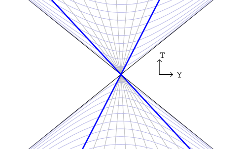
Figure 1: Comparing coordinate systems: In the near-brane limit, the two branes move along the lines $Y=Y_{\pm}(T)$ (thick lines). Lines of constant $y$ (straight) and $t$ (curved) are shown; $d(t)$ is the proper distance along a line of constant $t$ between the two branes. Note that, if $v_{+}\neq v_{-}$, the values of $T$ at either end of this line will be different. The coordinate system $(y,t)$ is only defined inside the lines $Y-Y_{0}=\pm n_{0}(T-T_{0})$ as shown

Note that this is in general not the same as other definitions of the radion, more common ones being the distance along integral curves of the normal (lines of constant $x$ are not in general geodesics in this metric, see Fig. 1) or, different again, $Y_{-}(T)-Y_{+}(T)$. When the effective theory is defined from a moduli space approximation, the radion often enters via a ratio of the conformal factors on the branes, but this is not meaningful apart from in the small-velocity limit. It is however of note that all these definitions are proportional in the special case of cosmological symmetry and small brane separation.

III Close branes effective theory description

III.1 Formalism

We work in a frame where the branes are assumed to be exactly static at $y=0,1$ with metric (15) in order to simplify the implementation of the Israël junction conditions, which would otherwise be difficult. From the Gauss equations, the Einstein tensor on a $y=\text{const}$ hypersurface is given by Binetruy:1999ut ; Shiromizu:1999wj :

$$G^{\mu}_{\nu}(y) = \frac{3}{L^{2}}\delta^{\mu}_{\nu}+KK^{\mu}_{\nu}-K^{\mu}_{\alpha}K^{\alpha}_{\nu}$$

$$-\frac{1}{2}\delta^{\mu}_{\nu}\left(K^{2}-K_{\alpha}^{\beta}K^{\alpha}_{\beta}\right)-E^{\mu}_{\nu}.$$

The unknown quantity in (III.1) is the electric part of the projected Weyl tensor $E^{\mu}_{\nu}$ which is traceless, enabling us to write the Ricci scalar purely in terms of the extrinsic curvature:

$$R=-\frac{12}{L^{2}}-K^{2}+K_{\alpha}^{\beta}K^{\alpha}_{\beta}.$$ (18)

The Weyl tensor $E^{\mu}_{\nu}$ can be expressed in terms of more recognisable quantities as

$$E^{\mu}_{\nu}=-\frac{1}{d}\frac{\partial}{\partial y}K^{\mu}_{\nu}-\frac{1}{d}D^{\mu}D_{\nu}d-K^{\mu}_{\alpha}K^{\alpha}_{\nu}+\frac{1}{L^{2}}\delta^{\mu}_{\nu},$$ (19)

where $D_{\mu}$ is the covariant derivative with respect to $q_{\mu\nu}(y)$, implying from (III.1) that:

$$G^{\mu}_{\nu}=\frac{1}{d} \Big{[}D^{\mu}D_{\nu}d+\frac{\partial}{\partial y}K^{\mu}_{\nu}$$

$$+\frac{2d}{L^{2}}\delta^{\mu}_{\nu}+dKK^{\mu}_{\nu}-\frac{d}{2}\delta^{\mu}_{\nu}\left(K^{2}-K_{\alpha}^{\beta}K^{\alpha}_{\beta}\right)\Big{]},$$

where the second line is of higher order in the small distance limit $d\ll L$.

In order to find the derivative of the extrinsic curvature $\frac{\partial}{\partial y}K^{\mu}_{\nu}$ on the brane, we consider the Taylor expansion:

$$K^{\mu}_{\nu}(y=1)=\sum_{n=0}^{\infty}\frac{1}{n!}\left.\partial_{y}^{(n)}K^{\mu}_{\nu}\right|_{y=0}.$$ (21)

We expand the $n^{\text{th}}$ derivative of the extrinsic curvature in powers of $d/L$, keeping only the leading term:

$$\left.\frac{\partial^{n}}{\partial y^{n}}K^{\mu}_{\nu}\right|_{y=0}\equiv K^{\mu\,(n)}_{\nu}=\mathcal{K}^{\mu\,(n)}_{\nu}\left(1+\mathcal{O}\left(\frac{d}{L}\right)\right)$$

and, as shown in Appendix A, one can obtain the recurrence relation

$$\mathcal{K}^{\mu\,(n)}_{\nu}=\hat{O}\mathcal{K}^{\mu\,(n-2)}_{\nu},$$ (22)

where the operator $\hat{O}$ is defined by

$$\hat{O}Z^{\mu}_{\nu}=\left[d^{,\mu}Z^{\alpha}_{\ \nu}+d_{,\nu}Z^{\alpha\mu}-d^{,\alpha}Z^{\mu}_{\ \nu}\right]d_{,\alpha},$$ (23)

giving

$$\sum_{n=0}^{\infty}\frac{1}{n!}\mathcal{K}^{\mu\,(n)}_{\nu} = \sum_{n=0}^{\infty}\frac{1}{(2n+1)!}\hat{O}^{n}\mathcal{K}^{\mu\,(1)}_{\nu}+\frac{1}{(2n)!}\hat{O}^{n}\mathcal{K}^{\mu\,(0)}_{\nu}$$ (24)

$$= \frac{\sinh\sqrt{\hat{O}}}{\sqrt{\hat{O}}}\ \mathcal{K}^{\mu\,(1)}_{\nu}+\cosh\sqrt{\hat{O}}\ \mathcal{K}^{\mu\,(0)}_{\nu}.$$

We then have a formal expression for the first derivative of the extrinsic curvature in terms of the radion and stress-energy:

$$\left.\frac{\partial}{\partial y}K^{\mu}_{\nu}\right|_{y=0}\sim-\frac{\sqrt{\hat{O}}}{\sinh\sqrt{\hat{O}}}\Big{[}\cosh\sqrt{\hat{O}}\,K^{(+)\mu}_{\phantom{(+)}\nu}-K^{(-)\mu}_{\phantom{(+)}\nu}\Big{]},$$ (25)

where $K^{(\pm)\mu}_{\phantom{(+)}\nu}=K^{\mu}_{\nu}(y=0,1)$. It is straightforward then to obtain the corresponding result for the negative-tension brane:

$$\left.\frac{\partial}{\partial y}K^{\mu}_{\nu}\right|_{y=1} = \left.\frac{\partial}{\partial y}K^{\mu}_{\nu}\right|_{y=0}+\sum_{n=2}^{\infty}\frac{K^{\mu(n)}_{\nu}}{\left(n-1\right)!}$$ (26)

$$\sim \left.\frac{\partial}{\partial y}K^{\mu}_{\nu}\right|_{y=0}+\left(\cosh\sqrt{\hat{O}}-1\right)\left.\frac{\partial}{\partial y}K^{\mu}_{\nu}\right|_{y=0}$$

$$\quad+\sinh\sqrt{\hat{O}}K^{(+)\mu}_{\phantom{(+)}\nu}$$

$$\sim \frac{\sqrt{\hat{O}}}{\sinh\sqrt{\hat{O}}}\Big{[}\cosh\sqrt{\hat{O}}\,K^{(-)\mu}_{\phantom{(+)}\nu}-K^{(+)\mu}_{\phantom{(+)}\nu}\Big{]}.$$

III.2 Einstein equations on the branes

The next step is to use the Israël junction conditons to rewrite the extrinsic curvatures of the two branes in terms of the stress-energy tensors and the tensions:

$$K^{(+)\mu}_{\phantom{(+)}\nu} = -\frac{1}{L}\delta^{\mu}_{\nu}-\frac{\kappa^{2}}{2}\hat{\tau}^{(+)\mu}_{\phantom{(+)}\nu}$$ (27)

$$K^{(-)\mu}_{\phantom{(+)}\nu} = -\frac{1}{L}\delta^{\mu}_{\nu}+\frac{\kappa^{2}}{2}\hat{\tau}^{(-)\mu}_{\phantom{(+)}\nu}$$ (28)

$$\hat{\tau}^{(\pm)\mu}_{\phantom{(+)}\nu} \equiv \tau^{(\pm)\mu}_{\phantom{(+)}\nu}-\frac{1}{3}\tau^{(\pm)}_{\phantom{(+)}}\delta^{\mu}_{\nu}.$$ (29)

This gives us both the value of the Ricci scalar on the branes (18)

$$R^{(\pm)}=\mp\frac{\kappa^{2}}{L}\tau^{(\pm)}+\frac{\kappa^{4}}{4}\left(\hat{\tau}^{(\pm)\,2}-\hat{\tau}^{(\pm)\,\alpha}_{\phantom{(\pm)}\,\beta}\hat{\tau}^{(\pm)\,\beta}_{\phantom{(\pm)}\,\alpha}\right)$$ (30)

and, substituting (25) (or (26)) into (III.1), the effective Einstein equations:

$$G^{(\pm)\mu}_{\phantom{(+)}\nu} \sim \frac{1}{d}D^{(\pm)\mu}D^{(\pm)}_{\phantom{(+)}\nu}d\pm\frac{1}{Ld}\left|\partial d\right|\tanh\frac{\left|\partial d\right|}{2}\delta^{\mu}_{\nu}$$

$$\pm\frac{1}{Ld}\frac{1}{\left|\partial d\right|}\left(\tanh\frac{\left|\partial d\right|}{2}+\tan\frac{\left|\partial d\right|}{2}\right)\partial^{\mu}d\,\partial_{\nu}d$$

$$+\frac{\kappa^{2}}{2d}\mathcal{A}^{(\pm)\mu}_{\phantom{(+)}\nu}$$

$$+\left[\pm\frac{2\kappa^{2}}{L}\left(\tau^{(\pm)\mu}_{\phantom{(+)}\nu}-\frac{\tau^{(\pm)}}{6}\delta^{\mu}_{\nu}\right)+\kappa^{4}\Pi^{(\pm)\mu}_{\phantom{(+)}\nu}\right],$$

where

$$\mathcal{A}^{(\pm)\mu}_{\phantom{(+)}\nu}=\sqrt{\hat{O}}\left(\coth\sqrt{\hat{O}}\hat{\tau}^{(\pm)\mu}_{\phantom{(+)}\nu}+\mathrm{cosech}\sqrt{\hat{O}}\hat{\tau}^{(\mp)\mu}_{\phantom{(+)}\nu}\right),$$ (32)

and

$$\Pi^{(\pm)\mu}_{\phantom{(+)}\nu}=\frac{1}{8}\tau^{(\pm)\alpha}_{\phantom{(+)}\beta}\tau^{(\pm)\beta}_{\phantom{(+)}\alpha}\delta^{\mu}_{\nu}-\frac{1}{12}\tau^{(\pm)}\tau^{(\pm)\mu}_{\phantom{(+)}\nu}-\frac{1}{72}\tau^{(\pm)\,2}\delta^{\mu}_{\nu}.$$ (33)

From the tracelessness of $E^{(\pm)}_{\mu\nu}$ we obtain two equivalent equations of motion for the radion,

$$\Box^{(\pm)}d \sim \mp\frac{\left|\partial d\right|}{L}\left(3\tanh\frac{\left|\partial d\right|}{2}-\tan\frac{\left|\partial d\right|}{2}\right)-\frac{\kappa^{2}}{2}\mathcal{A}^{(\pm)}$$

$$+\left[\pm\frac{\kappa^{2}d}{3L}\tau^{(\pm)}-\frac{\kappa^{4}d}{4}\hat{\tau}^{(\pm)\mu}_{\phantom{(+)}\nu}\hat{\tau}^{(\pm)\nu}_{\phantom{(+)}\mu}\right].$$

The terms in square brackets in (III.2) and (III.2) will turn out to be of higher order as $d\rightarrow 0$ and so should not strictly be included. However, for exact cosmological symmetry, they are the only higher order terms and we shall keep them for the time being. Later on they shall be discarded.

The conservation of the stress-energy tensor on both branes follows directly from the Codacci equation Binetruy:1999ut ; Shiromizu:1999wj :

$$D_{\mu}K^{\mu}_{\nu}-D_{\nu}K=0,$$ (35)

which, evaluated on the branes implies

$$D^{(+)}_{\mu}\tau^{(+)\mu}_{\phantom{(+)}\nu}=D^{(-)}_{\mu}\tau^{(-)\mu}_{\phantom{(+)}\nu}=0.$$ (36)

III.3 Low-energy limit

As a first consistency check of this close-brane theory, we consider its low-energy limit and compare it with the effective four-dimensional low-energy theory Mendes:2000wu ; Khoury:2002jq ; Kanno:2002ia ; Shiromizu:2002qr for small brane separation. In that common limit, both theories should agree.

In the low-energy limit, the magnitude of the stress-energy tensor on the brane is small compared to the brane tension. Any quadratic term $\kappa^{4}\tau^{(\pm)\,2}$ is negligible compared to $\frac{\kappa^{2}}{L}\tau^{(\pm)}$, so that $\Pi^{(\pm)\mu}_{\phantom{(\pm)}\nu}$ may be dropped in (III.2) and, from (30), the Ricci tensor on the brane is:

$$R^{(\pm)}=\mp\frac{\kappa^{2}}{L}\tau^{(\pm)}.$$ (37)

Furthermore in the low-energy limit, the branes are moving slowly, $\left|\partial d\right|\ll 1$, to linear order in $\left|\partial d\right|$, we have:

$$\mathcal{A}^{(\pm)\mu}_{\phantom{(+)}\nu}=\hat{\tau}^{(+)\mu}_{\phantom{(+)}\nu}+\hat{\tau}^{(-)\mu}_{\phantom{(+)}\nu}.$$ (38)

The effective Einstein equation on the brane at low energy is therefore

$$G^{(\pm)\mu}_{\phantom{(+)}\nu} \sim \frac{1}{d}D^{(\pm)\mu}D^{(\pm)}_{\nu}d+\frac{\kappa^{2}}{2d}\left(\hat{\tau}^{(+)\mu}_{\phantom{(+)}\nu}+\hat{\tau}^{(-)\mu}_{\phantom{(+)}\nu}\right)$$

$$\pm\frac{1}{Ld}\left(\partial^{\mu}d\,\partial_{\nu}d-\frac{1}{2}\left(\partial d\right)^{2}\delta^{\mu}_{\nu}\right),$$

with the equation of motion for $d$:

$$\Box^{(\pm)}d=\pm\frac{1}{L}\left(\partial d\right)^{2}+\frac{\kappa^{2}}{6}\left(\tau^{(+)}+\tau^{(-)}\right).$$ (40)

We can therefore write (III.3) in the more common form:

$$G^{(\pm)\mu}_{\phantom{(+)}\nu} \sim \frac{\kappa^{2}}{2d}\left(\tau^{(+)\mu}_{\phantom{(+)}\nu}+\tau^{(-)\mu}_{\phantom{(+)}\nu}\right)$$

$$+\frac{1}{d}\left(D^{(\pm)\mu}D^{(\pm)}_{\nu}d-\Box^{(\pm)}d\right)$$

$$\pm\frac{1}{Ld}\left(\partial^{\mu}d\,\partial_{\nu}d+\frac{1}{2}\left(\partial d\right)^{2}\delta^{\mu}_{\nu}\right),$$

which is precisely the result we get from the effective low-energy theory in the close brane limit Mendes:2000wu ; Khoury:2002jq ; Kanno:2002ia ; Shiromizu:2002qr ; deRham:2004yt .

IV Cosmological Symmetry

In the most general case, the coupling of the radion to matter on the branes given by (32) is intractable. However, we are concerned here with the case of cosmological symmetry as a check on the validity of the theory. We take (12) as our metric and notice that

$$\hat{O}\left(\begin{array}[]{cc}A&0\\ 0&B\,\delta^{i}_{j}\\ \end{array}\right)=\dot{d}^{2}\left(\begin{array}[]{rc}-A&0\\ 0&B\,\delta^{i}_{j}\\ \end{array}\right).$$ (46)

We can then obtain the coupling tensors (32) in closed form:

$$\mathcal{A}^{(\pm)0}_{\phantom{(+)}0} = -\dot{d}\cot\dot{d}\left(\frac{2}{3}\rho_{\pm}+p_{\pm}\right)$$

$$-\dot{d}\ \mathrm{cosec}\ \dot{d}\left(\frac{2}{3}\rho_{\mp}+p_{\mp}\right)$$

$$\mathcal{A}^{(\pm)i}_{\phantom{(+)}j} = \frac{\dot{d}}{3}\left(\rho_{\pm}\coth\ \dot{d}+\rho_{\mp}\mathrm{cosech}\ \dot{d}\right)\delta^{i}_{j}.$$ (48)

The resulting equations of motion follow from (III.2),(III.2) and (36):

$$H_{\pm}^{2} \sim \frac{1}{d}\left[-\dot{d}H_{\pm}\pm\frac{\dot{d}}{L}\tanh\frac{\dot{d}}{2}+\frac{\kappa^{2}}{6}\mathcal{A}^{(\pm)i}_{\phantom{(+)}i}\right]$$

$$\pm\frac{2\kappa^{2}}{3L}\rho_{\pm}+\frac{1}{18}\kappa^{4}\rho_{\pm}^{2}$$

$$\dot{H}_{\pm}+2H_{\pm}^{2} \sim \pm\frac{\kappa^{2}}{6L}\left(\rho_{\pm}-3p_{\pm}\right)-\frac{\kappa^{4}}{36}\rho_{\pm}\left(\rho_{\pm}+3p_{\pm}\right)$$ (50)

$$\ddot{d}+3H_{+}\dot{d} \sim \frac{\dot{d}}{L}\left(3\tanh\frac{\dot{d}}{2}-\tan\frac{\dot{d}}{2}\right)$$

$$+\frac{\kappa^{2}d}{L}\left(\frac{\rho_{+}}{3}-p_{+}\right)+\frac{\kappa^{2}}{2}\left(\mathcal{A}^{(+)0}_{\phantom{(+)}0}+\mathcal{A}^{(+)i}_{\phantom{(+)}i}\right)$$

$$+\frac{\kappa^{4}d}{4}\left(\frac{7}{9}\rho_{+}^{2}+p_{+}^{2}+\frac{4}{3}\rho_{+}p_{+}\right)$$

$$\dot{\rho}_{\pm} = -3H_{\pm}\left(\rho_{\pm}+p_{\pm}\right).$$ (52)

Equations (52) and (50) together imply

$$H_{\pm}^{2}\sim\frac{\tilde{\mathcal{C}}}{La_{\pm}^{4}}\pm\frac{\kappa^{2}}{3L}\rho_{\pm}+\frac{\kappa^{4}}{36}\rho_{\pm}^{2},$$ (53)

where $\tilde{\mathcal{C}}$ is an integration constant which, at this order, can be identified with the bulk parameter $\mathcal{C}$ via (7). The system is now manifestly finite as $d\rightarrow 0$. Note that, apart from the presence of quadratic terms, (50) is the same result as that obtained from the moduli space approximation and is, in fact, exact ($d$ decouples as a consequence of the simplicity of the Weyl tensor for an AdS-Schwarzschild bulk). However, the additional information from (IV) gives additional information not obtainable from a low-energy effective theory. Since $H_{+}$ takes a finite value at the collision, the coefficient of $d^{-1}$ in (IV) must vanish at $d=0$; this implies then that

$$H_{+}(0) = \frac{1}{L}\tanh\frac{\dot{d}(0)}{2}$$

$$+\frac{\kappa^{2}}{6}\left(\rho_{+}(0)\coth\ \dot{d}(0)+\rho_{-}(0)\mathrm{cosech}\ \dot{d}(0)\right),$$

in agreement with the exact result (II).

V Effective theory for perturbations

More interesting is the study of cosmological perturbations, for which a relatively straightforward solution of the above system is also available. We shall give a few examples here and point out some interesting features. Throughout we work only with the positive-tension brane, assuming the negative-tension brane to be empty, and drop the $\pm$ signs. Also, we shall assume for simplicity that matter on the positive-tension brane is only introduced at the perturbed level, i.e. the background solution $a(t),d(t)$ is that obtained from (50) and (IV) in the absence of matter. We therefore have

$$\begin{array}[]{cclcl}\tau^{\mu}_{\nu}(\mathbf{x},t)&=&0&+&\delta\tau^{\mu}_{\nu}\\ d(\mathbf{x},t)&=&d(t)&+&\delta d(\mathbf{x},t)\\ g_{\mu\nu}(\mathbf{x},t)&=&\bar{g}_{\mu\nu}&+&\delta g_{\mu\nu},\end{array}$$

where $\bar{g}_{\mu\nu}$ is the usual flat FRW metric with scale factor $a(t)$. However, in the following we will set $\delta d=0$, either because we are considering tensor perturbations only or because we choose to work in such a gauge. Hence we shall assume that $d$ takes its background value.

V.1 Tensor Perturbations

As the simplest starting point we consider perturbations using the above formalism and we choose to work in conformal time. We take the metric to be

$$\mathrm{d}s^{2}=a(\eta)^{2}\left(-\mathrm{d}\eta^{2}+\left(\delta_{ij}+h_{ij}\right)\mathrm{d}x^{i}\mathrm{d}x^{j}\right),$$ (55)

with the usual transverse traceless conditions

$$h^{i}_{i}=h^{i}_{j,i}=0$$

on the perturbation, spatial indices being raised by $\delta^{ij}$. The resulting Ricci tensor perturbation is then

$$\delta R_{00} = \delta R_{0i}=0,$$

$$\delta R_{ij} = \left(\mathcal{H}^{\prime}+2\mathcal{H}^{2}\right)h_{ij}+\mathcal{H}h^{\prime}_{ij}-\frac{1}{2}\bar{\Box}h_{ij},$$ (56)

where $\mathcal{H}=a^{\prime}/a=aH$, primes denote differentiation with respect to conformal time $\eta$ and $\bar{\Box}=-\partial_{\eta}^{2}+\partial_{i}\partial^{i}$ is the Minkowski space wave operator. We assume that these gravity waves are sourced by tensor matter at the perturbative level, i.e.

$$\delta\tau^{\mu}_{\nu}=\delta\hat{\tau}^{\mu}_{\nu}=\left(\begin{array}[]{cc}0&0\\ 0&\tau^{i}_{j}\end{array}\right),\qquad\tau^{i}_{i}=0.$$

The perturbed Klein Gordon equation for tensor matter just reduces to $\delta\left(\Box d\right)\sim 0$, so it is consistent to set the scalar perturbation $\delta d$ to zero, i.e. to study purely tensor fluctuations. In this case, the equation of motion for the perturbations follows from (III.2):

$$\delta R_{ij} \sim \frac{1}{d}\delta\left(D_{i}D_{j}\,d\right)+\frac{\dot{d}}{Ld}\tanh\frac{\dot{d}}{2}\ a^{2}h_{ij}$$

$$+\frac{\kappa^{2}}{2d}\sqrt{\hat{O}}\coth\sqrt{\hat{O}}\ \delta{\hat{\tau}}_{ij},$$

where we have now dropped the sub-dominant matter terms. It is straightforward to obtain

$$\delta\left(D_{i}D_{j}\,d\right) = -\left(\frac{1}{2}h^{\prime}_{ij}+\mathcal{H}h_{ij}\right)d^{\prime}$$

$$\sqrt{\hat{O}}\coth\sqrt{\hat{O}}\,\delta\hat{\tau}_{ij} = \dot{d}\coth\dot{d}\ \tau_{ij}.$$

Equations (IV) and (50) then imply the relation for the background Hubble parameter

$$\mathcal{H}^{\prime}+\mathcal{H}^{2}=0,\quad\mathcal{H}^{2}=-\frac{d^{\prime}}{d}\mathcal{H}+a^{2}\frac{\dot{d}}{L}\tanh\frac{\dot{d}}{L}.$$

Putting this all together we obtain, to leading order in $d$:

$$\hat{\boxdot}\,h_{ij}\equiv\left[\bar{\Box}-\frac{d^{\prime}}{d}\frac{\partial}{\partial\eta}\right]h_{ij}=-\kappa^{2}\frac{\dot{d}}{d}\coth\dot{d}\ \delta\tau_{ij}.$$ (58)

The same calculation repeated subject to the low-energy approximation, not assuming small $d$, is straightforward. Since the matter is traceless, the standard equations at low energy Mendes:2000wu ; Khoury:2002jq ; Kanno:2002ia ; Shiromizu:2002qr ; deRham:2004yt give

$$R_{ij}\approx\frac{1-\psi}{L^{2}\psi}\left(2LD^{(+)}_{i}\partial_{j}d-g_{ij}\partial d^{2}+2\partial_{i}d\partial_{j}d\right)+\frac{\kappa^{2}}{L\psi}\tau^{(+)}_{ij},$$

where $\psi=1-\exp\left(-2d/L\right)$. Perturbing this gives

$$\bar{\Box}h_{ij}-2\left[\mathcal{H}+\frac{\left(1-\psi\right)}{\psi}\frac{d^{\prime}}{L}\right]h^{\prime}_{ij}\approx-\frac{2\kappa^{2}}{L\psi}\delta\tau_{ij},$$ (59)

using the equations

$$\mathcal{H}^{\prime}+\mathcal{H}^{2}=0,\quad\mathcal{H}^{2}+2\frac{\left(1-\psi\right)}{L\psi}\mathcal{H}d^{\prime}\approx\frac{d^{\prime 2}}{L^{2}}\frac{\left(1-\psi\right)}{\psi},$$

for the background. The small-$d$ limit of (59), where $\psi\sim 2d/L$, is then

$$\bar{\Box}h_{ij}-\frac{d^{\prime}}{d}h^{\prime}_{ij}\sim-\frac{\kappa^{2}}{d}\delta\tau_{ij}.$$

The operator $\hat{\boxdot}$ defined in (58) is therefore the same as one would find in the low-energy theory. The difference lies in the source term; in the high-energy theory, the effective four-dimensional Newton constant on the positive-tension brane is related to the five-dimensional one by

$$\kappa^{(+)\,2}_{4d}=\frac{\dot{d}}{d}\coth\dot{d}\ \kappa^{2},$$ (60)

whereas the low-energy result has

$$\kappa^{(+)\,2}_{4d}\sim\frac{\kappa^{2}}{d_{0}}.$$ (61)

As is the case in the low-energy effective theory, the coupling to matter is different for the background as it is for the perturbations - for the background, the coupling can be identified from (8) or (53) as $\kappa^{2}/L$, as opposed to (60). When either the branes are stabilised, and $d$ is not treated as a dynamical variable, $d\sim d_{0}=\text{const}$, or the velocity is small $\dot{d}\ll 1$ (which is the case in the low-energy limit), it is easy to see that (60) and (61) agree. However, for arbitrary brane velocities, when the radion is not stabilised, the exact result for small $d$ is given by (60). As expected, the effective Newton constant picks up a dependence on $d$, as it does in the low-energy theory, but more unexpected, it also contains some degree of freedom: the brane separation velocity. Whilst this is not expected to be relevant today, since one would assume the radion is stabilised in the present Universe, it would be extremely important near the brane collision. As discussed in section II, $\dot{d}$ would be approximately constant, $\dot{d}\sim v$, leading to

$$\kappa^{(+)\,2}_{4d}\sim\frac{\coth v}{t}\,\kappa^{2},$$ (62)

where the coefficient $\coth v$ could take any value greater than $1$ depending on the matter content of the branes.

V.2 Scalar Perturbations

We now consider scalar metric perturbations on the brane sourced by a perfect fluid at the perturbative level (again, the background geometry is taken to be empty). We choose to work in a gauge where $\delta d=0$, i.e. to evaluate the perturbations on hypersurfaces of constant $d$, in which the metric perturbation can be taken as

$$\mathrm{d}s^{2} = a(\eta)^{2}\Big{(}\left(-1+2\Phi\right)\mathrm{d}\eta^{2}+4E_{,i}\mathrm{d}\eta\mathrm{d}x^{i}$$

$$\qquad\qquad+\left(1+2\Psi\right)\delta_{ij}\mathrm{d}x^{i}\mathrm{d}x^{j}\Big{)}.$$

The calculations are not nearly so straightforward as for tensors and have therefore been relegated to Appendix B. The result is the following equation of motion for the curvature perturbation

$$\hat{\boxdot}\,\Psi\equiv\left[\bar{\Box}-\frac{d^{\prime}}{d}\frac{\partial}{\partial\eta}\right]\Psi=-a^{2}\frac{\kappa^{2}}{6}\frac{\dot{d}}{d}\coth\dot{d}\ \delta\rho,$$ (64)

giving rise to the same relation between the four-dimensional Newtonian constant and the five-dimensional as in (60). Here again we may check that, apart from the modification of the effective Newtonian constant on the brane, the perturbations propagate in the given background exactly the same way as they would if the theory were genuinely four-dimensional. This is a very important result for the propagation of scalar perturbations if they are to generate the observed large-scale structure. The five-dimensional nature of the theory does affect the background behaviour but on this background the perturbations behave exactly the same way as they would in the four-dimensional theory.

This result is of course only true in the close-brane limit, for which the theory contains no higher than second derivatives, only powers of first derivatives. When the branes are no longer very close to each other, the theory will become higher-dimensional (in particular the theory becomes non-local in the one brane limit). The presence of these higher-derivative corrections (not expressible as powers of first derivatives) is expected to modify the way perturbations propagate in a given background, mainly because extra Cauchy data would need to be specified, making the perturbations non adiabatic deRham:2004yt . However if we consider a scenario for which the large-scale structure is generated just after the brane collision, the mechanism for the production of the scalar perturbations will be very similar to the standard four-dimensional one.

V.3 Relation between the four- and five-dimensional Newtonian constant

The relation (60) between $\kappa_{4d}^{(+)\,2}$ and the five-dimensional constant $\kappa^{2}$ is formally only valid for small distance between the branes. However if we consider the analysis of deRham:2005xv , we may have some insights of what will happen if we had not stopped the expansion to leading order in $d$. Here, terms of the form $d\,\ddot{d}$ and more generally any term of the form $d^{n}d^{(n+1)}$ have been considered as negligible in comparison to $\dot{d}$ and therefore only the terms of the form $\dot{d}^{n}$ have been considered in the expansion. In a more general case, when the branes are not assumed to be very close to each other, any term of the form $d^{n}\,d^{(n+1)}$ should be considered and would affect the relation between the four-dimensional Newtonian constant and the five-dimensional one. For moving branes, we therefore expect the relation between $\kappa_{4d}^{(+)\,2}$ and $\kappa^{2}$ to be:

$$\kappa_{4d}^{(+)\,2}=\frac{\kappa^{2}}{L}\ \Omega\left(\frac{d}{L},\dot{d},d\,\ddot{d},\cdots,d^{n}\,d^{(n+1)}\right).$$ (65)

The relation is therefore a functional of $d$: $\Omega\left[d(t)\right]$ has an infinite number of independent degree of freedom.

In the low-energy limit, or when the radion is stabilised, $d\sim d_{0}=\text{const}$, the exact expression of $\Omega$ is Garriga:1999yh :

$$\Omega\rightarrow\Omega\left[d(t)=d_{0}\right]=\frac{e^{d_{0}/L}}{2\sinh d_{0}/L}$$ (66)

For close branes, another limit is now known: when $d\ll L$,

$$\Omega\left[d\ll L\right]=\frac{\dot{d}}{d}\coth\dot{d}.$$ (67)

But in a general case, $\Omega$ (and therefore $\kappa_{4d}^{(+)\,2}$) is expected to be a completely dynamical degree of freedom. For the present Universe the radion is supposed to be stabilised, but in early-Universe cosmology, the effective four-dimensional Newton constant could be very different from its present value. It might therefore be interesting to understand what the constraints on such time-variation of the Newtonian constant would be and how it would constrain the brane velocity Clifton:2005xr ; Barrow:1996kc , or whether such a time variation could act as a signature for the presence of extra dimensions.

VI Conclusions

In the first part of this work, we derived the exact behaviour of FRW branes in the presence of matter. The characteristic features come from the presence of the $\rho^{2}$ terms in the Friedmann equation and from the ‘dark energy’ Weyl term. In the limit of close separation we related the contribution of the Weyl term to the expansion of the fifth dimension. We then used this result to test the close-brane effective theory that was first derived in deRham:2005xv but now with matter introduced on the branes. For this we have shown how matter can be included using a formal sum of operators acting on the stress-energy tensors for matter fields on both branes. In the general case the action of this sum of operators on an arbitrary stress-energy tensor would not be available in closed form, although one could in principle proceed perturbatively. When a specific scenario is chosen, however, one can make considerable analytical progress. Assuming cosmological symmetry, the action of the operators on the stress-energy tensor is remarkably simple and the sum can be evaluated analytically. We then compared the result with the exact five-dimensional result in the limit of small brane separation. As expected both results agree perfectly. Furthermore we have checked that, in the low-energy limit, our close-brane effective theory agrees perfectly with the effective four-dimensional low-energy theory, giving another consistency check.

We then used this close-brane effective theory in order to understand the way matter couples to gravity at the perturbed level. In order to do so, we considered a scenario in the stiff source approximation for which the background is supposed to be unaffected by the presence of matter and considered the production of curvature and tensor perturbation sourced by the presence of matter fields on the brane. Although the five-dimensional nature of the theory does affect the background behaviour, we have shown that for a given background the perturbations propagate the same way as they would in a standard four-dimensional theory. This is only true in the limit of small brane separation and is not expected to be valid outside this regime. However, since the large-scale structure of the Universe might have been produced in a period for which the branes could have been close together (for instance just after a brane collision initiating the Big Bang), this regime is of special interest. The fact that the perturbations behave the same way, for a given background, as they would in a four-dimensional theory is a remarkable result for the production of the large scale structure which could be almost unaffected by the presence of the fifth dimension. On the other hand, the relation between the four-dimensional Newtonian constant and the five-dimensional one is however affected by the expansion of the fifth-dimension. It has been shown in the literature Randall:1999ee ; Garriga:1999yh that four-dimensional Newtonian constant was dependant on the distance between the branes, giving a possible explanation of the hierarchy problem. In this paper we show that the four-dimensional Newtonian constant also has some dependence on the brane velocity which we computed exactly in the small-distance limit, which might be able to provide an observational signature for the presence of extra dimensions. Outside the small $d$ regime, we expect the four-dimensional Newtonian constant to depend on the five-dimensional one not only through the brane separation velocity $\dot{d}$ but also on higher derivatives of the distance between the branes $d^{(n)}$, making the requirement for moduli stabilisation even more fundamental for any realistic cosmological setup within braneworld cosmology.

VII Acknowledgements

The authors would like to thank Anne Davis for her supervision and comments on the manuscript and Andrew Tolley for useful discussions. SLW is supported by PPARC and CdR by DAMTP.

Appendix A Leading order derivative of the extrinsic curvature

In this appendix, we shall derive an expression for the derivative of the extrinsic curvature on he branes. We will not be able to calculate these quantities exactly, but will be able to obtain a relatively simple expression for its leading-order contribution. We will focus on the positive-tension brane first, and our starting point shall be the Taylor series

$$K^{(-)\mu}_{\phantom{(+)}\nu}=\sum_{n=0}^{\infty}\frac{1}{n!}K^{\mu(n)}_{\nu},$$ (68)

where we are defining

$$K^{\mu\,(n)}_{\nu}\equiv\left.\frac{\partial^{n}}{\partial y^{n}}K^{\mu}_{\nu}\right|_{y=0}.$$

We are interested only in the leading order contribution to $K^{\mu(n)}_{\nu}$,

$$K^{\mu(n)}_{\nu}=\mathcal{K}^{\mu(n)}_{\nu}\left(1+\mathcal{O}\left(d/L\right)\right),$$

and the aim of this section will be to establish that

$$\mathcal{K}^{\mu(n)}_{\nu}=\hat{O}\mathcal{K}^{\mu(n-2)}_{\nu},$$ (69)

where the operator $\hat{O}$ is defined by

$$\hat{O}Z^{\mu}_{\nu} \equiv \left[d^{,\mu}Z^{\alpha}_{\ \nu}+d_{,\nu}Z^{\alpha\mu}-d^{,\alpha}Z^{\mu}_{\ \nu}\right]d_{,\alpha}.$$

This implies that $\mathcal{K}^{\mu(n)}_{\nu}$ is of the same order as $\mathcal{K}^{\mu(n-2)}_{\nu}$, and will allow us to produce a simple, albeit formal, expression for this sum, which will be the starting point for writing down the small-$d$ effective theory in the next section. We will proceed by induction, and throughout make the following assumptions about the order of terms:

• $\partial_{\mu}\partial_{\nu}d\sim\partial_{\nu}d\sim d^{0}$

• $\tau^{(+)\mu}_{\phantom{(+)}\nu}$, $D^{(+)}_{\alpha}\tau^{(+)\mu}_{\phantom{(+)}\nu}$ are at worst as divergent as the geometry

• $E^{(+)\mu}_{\phantom{(+)}\nu}\sim d^{-1}$.

The assumption on the order of magnitude of the matter terms is reasonable, since the matter introduced on the brane is expected to scale as the scale factor for the background and as the curvature perturbation for general perturbations. Since the curvature perturbations is in general expected to diverge logarithmically at the collision, we can hence assume that $\tau^{(+)\mu}_{\phantom{(+)}\nu}$, is, at worst, logarithmically divergent in $d$. This implies that the extrinsic curvature on the brane is itself at worse logarithmically divergent in $d$. Similarly, we know that $E^{(+)\mu}_{\phantom{(+)}\nu}\sim d^{-1}$ for the low-energy theory. Although we have argued that at high energy the moduli space approximation does not give the exact expression for the Weyl tensor, we have seen that (at least for the background) the behaviour is the same, differing only in corrections at higher order in the velocity. In particular $E^{\mu}_{\nu}$ should go as $d^{-1}$ at high energies as well (we will see later that this is indeed the case). From (19) we have

$$K^{\mu(1)}_{\nu} = -dE^{\mu}_{\nu}\left(y=0\right)\ -\left.D^{\mu}\partial_{\nu}d\right|_{y=0}$$ (70)

$$-\frac{\kappa^{2}d}{L}\tau^{(+)\mu}_{\phantom{(+)}\nu}-\frac{\kappa^{4}}{4}d\hat{\tau}^{(+)\mu}_{\phantom{(+)}\alpha}\hat{\tau}^{(-)\alpha}_{\phantom{(+)}\nu}$$

which, from the above assumptions, gives us

$$\mathcal{K}^{\mu(1)}_{\nu}\sim d^{0}.$$ (71)

For the second derivative of the extrinsic curvature, i.e. for $n=2$, we need expressions for the derivatives of the Weyl tensor and the Christoffel symbols. It is straightforward to show that

$$\Gamma^{\,\alpha\,\prime}_{\mu\nu}=D_{\mu}(d\,K^{\alpha}_{\nu})+D_{\nu}(d\,K^{\alpha}_{\mu})-D^{\alpha}(d\,K_{\mu\nu}),$$ (72)

and the derivative of the Weyl tensor is deRham:2005xv

$$E^{\mu\,\prime}_{\ \nu} = d\Big{(}2K^{\alpha}_{\nu}E^{\mu}_{\alpha}-\frac{3}{2}KE^{\mu}_{\nu}-\frac{1}{2}K^{\alpha}_{\beta}E^{\beta}_{\alpha}\delta^{\mu}_{\nu}+C^{\mu}_{\phantom{\mu}\alpha\nu\beta}K^{\alpha\beta}$$

$$2\hat{K}^{\alpha}_{\mu}\hat{K}_{\alpha\beta}\hat{K}^{\alpha}_{\nu}-\frac{7}{6}\hat{K}_{\alpha\beta}\hat{K}^{\alpha\beta}\hat{K}_{\mu\nu}-\frac{1}{2}q_{\mu\nu}\hat{K}_{\alpha\beta}\hat{K}^{\beta}_{\rho}\hat{K}^{\alpha\rho}\Big{)}$$

$$-\frac{1}{2d}D^{\alpha}\left[d^{2}D^{\mu}K_{\alpha\nu}+d^{2}D_{\nu}K^{\mu}_{\alpha}-2d^{2}D_{\alpha}K^{\mu}_{\nu}\right],$$

where $\hat{K}^{\mu}_{\nu}=K^{\mu}_{\nu}-\frac{1}{4}K\delta^{\mu}_{\nu}$. On the brane, from the Israël matching conditions, the trace of the extrinsic curvature is $K\sim\tau$, hence $\hat{K}^{\mu}_{\nu}\sim\tau$ also. So the cubic terms in $\hat{K}$ will be of higher order than the $KE$ terms, as will the $CK$ term. The leading terms will, in fact, just be the first three, giving

$${E^{\mu}_{\nu}}^{\prime}(0)\sim\frac{4d}{L}E^{\mu}_{\nu}(0).$$ (74)

On the brane,

$$D^{(+)}_{\alpha}\left(dK^{(+)\mu}_{\phantom{(+)}\nu}\right) = \left(\partial_{\alpha}d\right)K^{(+)\mu}_{\phantom{(+)}\nu}+dD^{(+)}_{\alpha}K^{(+)\mu}_{\phantom{(+)}\nu}$$ (75)

$$\sim \left(\partial_{\alpha}d\right)K^{(+)\mu}_{\phantom{(+)}\nu},$$

the second term being subdominant from the assumption that $D^{(+)}_{\alpha}K^{(+)\mu}_{\phantom{(+)}\nu}\propto D^{(+)}_{\alpha}\hat{\tau}^{(+)\mu}_{\phantom{(+)}\nu}$ is of higher order than $d^{-1}$. The derivative of the Christoffel symbol will similarly be of the same order as the extrinsic curvature on the brane:

$$\Gamma^{\,\alpha\,\prime}_{\mu\nu}(0)\sim\left(d_{,\mu}K^{(+)\alpha}_{\phantom{(+)}\nu}+d_{,\nu}K^{(+)\alpha}_{\phantom{(+)}\mu}-d^{,\alpha}K^{(+)}_{\mu\nu}\right).$$ (76)

Taking the derivative of (19) gives

$${K^{\mu}_{\nu}}^{\prime\prime}(y) = -d{E^{\mu}_{\nu}}^{\prime}+2dK^{\mu\beta}D_{\beta}\partial_{\nu}d+q^{\mu\beta}\Gamma^{\,\alpha\,\prime}_{\beta\nu}\partial_{\alpha}d$$ (77)

$$-d\ \partial_{y}\left(K^{\mu}_{\alpha}K^{\alpha}_{\nu}\right),$$

in the bulk. Evaluated on the brane using (74) and (76), the dominant term (of order $d^{0}$) is the one containing the derivative of the Christoffel symbol

$$K^{\mu(2)}_{\nu} \sim q^{(+)\mu\beta}\Gamma^{\alpha\,\prime}_{\beta\nu}(0)\partial_{\alpha}d\sim K.$$ (78)

Since we have shown in (76) that $\Gamma^{\alpha\,\prime}_{\beta\nu}(0)\sim d_{,\beta}K^{(+)\alpha}_{\phantom{(+)}\nu}$, on the brane, the second derivative of the extrinsic curvature is hence of the same order as the extrinsic curvature itself $K^{\mu(2)}_{\nu}\sim K^{\mu}_{\nu}$.

Using (76), we have proved the result for $n=2$:

$$\mathcal{K}^{\mu(2)}_{\nu} = d_{,\alpha}\left[d^{,\mu}K^{(+)\alpha}_{\phantom{(+)}\nu}+d_{,\nu}K^{(+)\alpha\mu}-d^{,\alpha}K^{(+)}_{\mu\nu}\right]$$ (79)

$$\sim \hat{O}K^{(+)\mu}_{\phantom{(+)}\nu}.$$

The second derivative of the Christoffel symbol follows from (72):

$$\Gamma^{\,\alpha\ \prime\prime}_{\mu\nu}(y) = D_{\mu}\left(d\,K^{\alpha\,\prime}_{\,\nu}\right)+D_{\nu}\left(d\,K^{\alpha\,\prime}_{\,\mu}\right)-D^{\alpha}\left(d\,K^{\prime}_{\mu\nu}\right)$$

$$+d\,\left(\Gamma^{\,\alpha\,\prime}_{\mu\rho}K^{\rho}_{\nu}+\Gamma^{\,\alpha\,\prime}_{\nu\rho}K^{\rho}_{\mu}-2\Gamma^{\,\rho\,\prime}_{\mu\nu}K^{\alpha}_{\rho}\right)$$

$$-d\,q^{\alpha\beta}q_{\mu\sigma}\,\left(\Gamma^{\,\sigma\,\prime}_{\beta\rho}K^{\rho}_{\nu}-\Gamma^{\,\rho\,\prime}_{\beta\nu}K^{\sigma}_{\rho}\right)$$

$$-d\,\left(q^{\alpha\beta}q_{\mu\sigma}\right)^{\prime}\,\left(\Gamma^{\,\sigma}_{\beta\rho}K^{\rho}_{\nu}-\Gamma^{\,\rho}_{\beta\nu}K^{\sigma}_{\rho}\right)$$

where, recall, ${K^{\mu}_{\nu}}^{\prime}=d\mathcal{L}_{n}K^{\mu}_{\nu}$ is a tensor, hence the use of covariant derivatives. These $D(dK^{\prime})$ terms are of order $d^{0}$, whilst the others are all of higher order, when evaluated on the brane. The leading term is

$$\Gamma^{\,\alpha\,\prime\prime}_{\mu\nu}(0) \sim \partial_{\mu}d\,K^{\alpha\,\prime}_{\,\nu}(0)+\partial_{\nu}d\,K^{\alpha\,\prime}_{\,\mu}(0)-\partial^{\alpha}d\,K^{\prime}_{\mu\nu}(0)$$ (81)

$$\sim d^{0}.$$

Substituting (A) into (77) gives a complicated second-order differential equation for $K^{\mu}_{\nu}$. Taking repeated $y$-derivatives of this equation would be impractical, but to start with all we want to do is to work to leading order. We will first identify which term is dominant, before actually evaluating it. We therefore drop all indices and numerical factors for the time being, writing $q$ for the metric (with indices in any position), $K$ for $K^{\mu}_{\nu}$ and $\partial$ for $\partial_{\mu}$. For example, $q^{\prime}_{{\mu\nu}}\propto dK_{\mu\nu}=dq_{\mu\sigma}K^{\sigma}_{\nu}$ and so we would write $q^{\prime}=dqK$. The equation for $K^{\prime\prime}$ can then be written symbolically as

$$K^{\prime\prime} = d\,\left(\partial^{2}+\Gamma\partial+\partial\Gamma+\Gamma^{2}\right)q^{\prime}+dK^{3}+dK$$

$$+dKK^{\prime}+q\,\partial d\left(\Gamma^{\prime}+d\,\Gamma K+d\,\partial K\right)+\partial^{2}d\,q^{\prime},$$

and, from (78), we already know that the dominant term is $q\,\partial d\,\Gamma^{\prime}\sim K$. We know that $K^{(m)}(0)$ and $\Gamma^{(m)}(0)$ are all of order $d^{0}$ or $K(0)$ for $m=0,1,2$. Recalling that the extrinsic curvature on the brane is at worse logarithmically divergent in $d$, terms of the form $d\,K(0)$ will hence be negligible compared to terms of order $d^{0}$ (and of course compared to terms of order $K(0)$). Compared to the $d^{-1}$ divergence, $K(0)$ is hence still negligible. In what follows, terms of order $d^{0}$ (such as $K^{\prime}(0)$, $\Gamma(0)$ and $\Gamma^{\prime\prime}(0)$) and terms of order $K(0)$ (such as $K(0)$, $K^{\prime\prime}(0)$ and $\Gamma^{\prime}(0)$) can hence be treated in a similar way. Since they are all at worse going as $K(0)$, we shall use in what follows the notation $K^{(m)}(0)\sim\Gamma^{(m)}(0)\sim K(0)$ for $m=0,1,2$. We shall hence take as the inductive hypothesis that this result is true for all $m\leq n$. In particular,

$$\Gamma^{(m)}(0) \sim K(0)\quad\forall\ 0\leq m\leq n$$

$$q^{(m+1)}(0) \sim d\,K(0)\quad\forall\ 0\leq m\leq n$$

$$q(0) \sim d^{0}.$$

Writing $l=n-1$, we have

$$K^{(n+1)}=\partial_{y}^{(l)}K^{\prime\prime}$$ (83)

$$\phantom{K^{(n+1)}}=\partial_{y}^{(l)}\Big{[}d\left(\partial^{2}+\Gamma\partial+\partial\Gamma+\Gamma^{2}\right)q^{\prime}$$

$$\phantom{K^{(n+1)}\partial_{y}^{(l)}}+dK^{3}+dK+dKK^{\prime}+\partial^{2}d\,q^{\prime}$$

$$\phantom{K^{(n+1)}\partial_{y}^{(l)}}+q\,\partial d\left(\Gamma^{\prime}+d\,\Gamma K+d\,\partial K\right)\Big{]}.$$

Now, evaluating on the brane, we examine the order of each of these terms to find which is the dominant. For example, remembering that $\partial$ and $\partial_{y}$ commute, we have for $l\geq 0$,

$$\partial_{y}^{(l)}\left.\left(d\partial^{2}q^{\prime}\right)\right|_{y=0}=d\partial^{2}\left(q^{(n)}(0)\right)\sim dK(0)$$

and similarly

$$\left.\partial_{y}^{(l)}\Big{(}d\,\left(\Gamma\partial+\partial\Gamma+\Gamma^{2}\right)q^{\prime}+d\,K^{3}+d\,K\Big{)}\right|_{y=0} \sim d\,K(0)$$

$$\left.\partial_{y}^{(l)}\Big{(}d\,KK^{\prime}+q\partial d\,\left(d\Gamma K+d\partial K\right)+\partial^{2}d\,q^{\prime}\Big{)}\right|_{y=0} \sim d\,K(0).$$

Finally,

$$\left.\partial_{y}^{(l)}\left(q\Gamma^{\prime}\partial d\right)\right|_{y=0}=\partial d\,\sum_{m=0}^{l}\Big{(}\begin{array}[]{c}m\\ l\end{array}\Big{)}q^{(l-m)}(0)\Gamma^{(l+1)}(0),$$

and the $l=0$ term dominates this last sum, being of order $K(0)$. Hence the dominant term in the expression for $K^{\mu(n+1)}_{\nu}$ is, as in the $K^{\mu(2)}_{\nu}$ case, the one with the derivative of the Christoffel symbol, of the same order as $K(0)$.

We have now proved half of the inductive hypothesis, but still need to show that $\Gamma^{(n+1)}(0)\sim K(0)$. From (72), we have

$$\Gamma^{\,\alpha\,(n+1)}_{\mu\nu}(y)= \partial_{\mu}(d\,K^{\alpha(n)}_{\nu})+\partial_{\nu}(d\,K^{\alpha(n)}_{\mu})-\partial^{\alpha}(d\,K^{(n)}_{\mu\nu})$$ (87)

$$+d\,\partial_{y}^{(n)}\Big{[}\Gamma K\ \mathrm{terms}]$$

$$-\,\sum_{m=0}^{n-1}\Big{(}\begin{array}[]{c}m\\ n-1\end{array}\Big{)}\left(dK^{\rho\,(m)}_{\,\nu}\right)_{,\,\beta}\partial_{y}^{(n-m)}\left(q^{\alpha\beta}q_{\mu\rho}\right).$$

By the inductive hypothesis

$$d\partial_{y}^{(n)}\left(\Gamma K\right)\sim d\,K(0),\qquad\partial_{y}^{(n-m)}\left(q^{\alpha\beta}_{\mu\rho}\right)\sim d\,K(0)\ \ n>m$$

and

$$\partial_{\alpha}\left(dK^{\mu(n)}_{\nu}\right)=d_{,\alpha}K^{\mu(n)}_{\nu}+\mathcal{O}(d\,K(0)).$$

Therefore we can now read off from (87) the leading order contribution to $\Gamma^{(n)}$,

$$\Gamma^{\,\alpha\,(n+1)}_{\mu\nu}(0) = d_{,\mu}K^{\alpha\,(n)}_{\,\nu}+d_{,\nu}K^{\alpha\,(n)}_{\,\mu}-d^{,\alpha}K^{(n)}_{\mu\nu}$$ (88)

$$\sim K(0),$$

which agrees with (81) and proves the inductive hypothesis.

We are now finally in a position to calculate $\mathcal{K}^{\mu(n)}_{\nu}$ for general $n$. We know that the leading contribution obtained from repeatedly differentiating the right-hand side of (77) is

$$K^{\mu(n)}_{\nu}\sim q^{\mu\beta}\Gamma^{\,\alpha\,(n-1)}_{\beta\nu}\partial_{\alpha}d$$

which, from (88), immediately gives (69) and the result is proved.

Appendix B Scalar Perturbations in an FRW background

In this appendix, we shall present some of the details for the calculation of scalar perturbations of section V.2, with the metric perturbation as given in (V.2). We recall that we picked the comoving gauge for which $\delta d=0$. In that gauge we then have:

$$\delta\left|\partial d\right|=\dot{d}\Phi$$

Terms that appear to be sub-dominant will only be dropped at the end. Using (30), we get:

$$\delta R=\frac{\kappa^{2}}{L}\left(\delta\rho-3\delta p\right).$$ (89)

Since $a^{\prime\prime}=0$ for the background (we assume the brane to be empty), (89) implies

$$\Psi^{\prime\prime} + \frac{a^{\prime}}{a}\left(2k^{2}\,E+\Phi^{\prime}+3\Psi^{\prime}\right)$$

$$+ \frac{k^{2}}{3}\left(2\Psi+2E^{\prime}-\Phi\right)=\frac{\kappa^{2}}{6L}a^{2}\left(\delta\rho-3\delta p\right).$$

We now perturb (III.2), writing

$$z = \left|\partial d\right|$$

$$f(z) = z\tanh(z/2)$$

$$g(z) = \frac{1}{z}\left(\tanh(z/2)+\tan(z/2)\right)$$

for simplicity. The $ij$ (with $i\neq j$) component of the Einstein equation, to first order in the perturbations, reduces to:

$$\Phi-\Psi-2E^{\prime}=\left(4\frac{a^{\prime}}{a}+2\frac{d^{\prime}}{d}\right)E,$$ (91)

and the $0i$-component to:

$$\Psi^{\prime}=-\left(\frac{a^{\prime}}{a}+\frac{d^{\prime}}{2d}\right)\Phi.$$ (92)

So far these equations are equivalent to those one would have obtained in the low-energy limit. The difference comes from the $00$-component of the perturbed Einstein equations:

$$\frac{d^{\prime}}{d}\Phi^{\prime}+\frac{a^{2}}{Ld}\left(2f-\dot{d}f^{\prime}+\dot{d}^{3}g^{\prime}\right)\Phi-2k^{2}\Psi-6\mathcal{H}\Psi^{\prime}$$

$$\hskip 10.0pt-4k^{2}\mathcal{H}E=-\frac{\kappa^{2}}{6}a\frac{d^{\prime}}{d}\cot\dot{d}\left(2\delta\rho+3\delta p\right)$$ (93)

and from the equation of motion for $d$:

$$\Phi^{\prime}+\left(8\frac{d^{\prime}a^{\prime 2}}{L}f+\frac{a}{L}\left(g^{\prime}\dot{d}^{2}-4f^{\prime}\right)\right)\Phi+3\Psi^{\prime}$$ (94)

$$\hskip 10.0pt+2k^{2}E=-\frac{\kappa^{2}}{6}a\left(\cot\dot{d}\left(2\delta\rho+3\delta p\right)-3\coth\dot{d}\,\delta\rho\right).$$

Note that one must, at this order, treat $\Phi$,$\Phi^{\prime}$,$\Psi$ and $\Psi^{\prime}$ as four independent variables; differentiation with respect to conformal time will miss terms arising from higher order in $d$, since $d$ and $d^{\prime}$ are of different order. We must then solve the five equations (B-94) simultaneously. Using (91) to eliminate $\Phi$ from (B), we obtain

$$4k^{2}\left(\frac{d^{\prime}}{d}-\mathcal{H}\right)E = 6\,\Psi^{\prime\prime}+2k^{2}\Psi+6\mathcal{H}\left(\Phi^{\prime}+3\Psi^{\prime}\right)\hskip 15.0pt$$

$$-\frac{\kappa^{2}}{L}a^{2}\left(\delta\rho-3\delta p\right)$$

We may use a combination of (93) and (94) to find an expression for $\Phi^{\prime}$ in terms of $\Phi,\Psi,\rho$ and $p$ and hence write $E$ in terms of $\Psi,\Psi^{\prime},\Psi^{\prime\prime},\rho$ and $p$. This can then be used in (93) to obtain a complicated expression for $\Psi$ in terms of $\Psi^{\prime}$,$\Psi^{\prime\prime}$,$\delta\rho$ and $\delta p$. We then only keep the leading order in $d$ for each coefficient, resulting in the much simplified equation

$$\Psi^{\prime\prime}+\frac{d^{\prime}}{d}\Psi^{\prime}+k^{2}\Psi=\frac{\kappa^{2}}{6}a^{2}\frac{\dot{d}}{d}\coth\dot{d}\ \delta\rho.$$ (96)

References

- (1) C. de Rham and S. Webster, Phys. Rev. D 71 (2005) 123025 arXiv:hep-th/0504128.
- (2) T. Kaluza, Sitzungsber. Preuss. Akad. Wiss. Berlin (Math. Phys. ) 1921 (1921) 966.
- (3) O. Klein, Z. Phys. 37 (1926) 895 [Surveys High Energ. Phys. 5 (1986) 241].
- (4) I. Antoniadis, Phys. Lett. B 246, 377 (1990).
- (5) G. W. Gibbons and D. L. Wiltshire, Nucl. Phys. B 287 (1987) 717 [arXiv:hep-th/0109093].
- (6) P. Brax, C. van de Bruck and A. C. Davis, Rept. Prog. Phys. 67 (2004) 2183 [arXiv:hep-th/0404011].
- (7) A. C. Davis, P. Brax and C. van de Bruck, arXiv:astro-ph/0503467.
- (8) D. Langlois, Prog. Theor. Phys. Suppl. 148 (2003) 181 [arXiv:hep-th/0209261].
- (9) L. Randall and R. Sundrum, Phys. Rev. Lett. 83 (1999) 3370 [arXiv:hep-ph/9905221].
- (10) L. E. Mendes and A. Mazumdar, Phys. Lett. B 501 (2001) 249 [arXiv:gr-qc/0009017].
- (11) J. Khoury and R. J. Zhang, Phys. Rev. Lett. 89 (2002) 061302 [arXiv:hep-th/0203274].
- (12) S. Kanno and J. Soda, Phys. Rev. D 66 (2002) 083506 [arXiv:hep-th/0207029].
- (13) T. Shiromizu and K. Koyama, Phys. Rev. D 67 (2003) 084022 [arXiv:hep-th/0210066].
- (14) D. Langlois, Astrophys. Space Sci. 283 (2003) 469 [arXiv:astro-ph/0301022].
- (15) R. Maartens, D. Wands, B. A. Bassett and I. Heard, Phys. Rev. D 62 (2000) 041301 [arXiv:hep-ph/9912464].
- (16) D. Langlois, R. Maartens and D. Wands, Phys. Lett. B 489 (2000) 259 [arXiv:hep-th/0006007].
- (17) A. R. Liddle and A. N. Taylor, Phys. Rev. D 65 (2002) 041301 [arXiv:astro-ph/0109412].
- (18) R. Maartens, Living Rev. Rel. 7 (2004) 7 [arXiv:gr-qc/0312059].
- (19) K. Koyama, D. Langlois, R. Maartens and D. Wands, JCAP 0411 (2004) 002 [arXiv:hep-th/0408222].
- (20) C. de Rham, Phys. Rev. D 71 (2005) 024015 [arXiv:hep-th/0411021].
- (21) G. Calcagni, JCAP 0311, 009 (2003) [arXiv:hep-ph/0310304].
- (22) G. Calcagni, Phys. Rev. D 69, 103508 (2004) [arXiv:hep-ph/0402126].
- (23) E. Papantonopoulos and V. Zamarias, JCAP 0410 (2004) 001 [arXiv:gr-qc/0403090].
- (24) K. E. Kunze, Phys. Lett. B 587 (2004) 1 [arXiv:hep-th/0310200].
- (25) A. R. Liddle and A. J. Smith, Phys. Rev. D 68 (2003) 061301 [arXiv:astro-ph/0307017].
- (26) E. J. Copeland, A. R. Liddle and J. E. Lidsey, Phys. Rev. D 64 (2001) 023509 [arXiv:astro-ph/0006421].
- (27) M. Sami, N. Dadhich and T. Shiromizu, Phys. Lett. B 568 (2003) 118 [arXiv:hep-th/0304187].
- (28) T. Shiromizu, K. Koyama and K. Takahashi, Phys. Rev. D 67 (2003) 104011 [arXiv:hep-th/0212331].
- (29) T. Shiromizu, K. i. Maeda and M. Sasaki, Phys. Rev. D 62 (2000) 024012 [arXiv:gr-qc/9910076].
- (30) P. Binetruy, C. Deffayet, U. Ellwanger and D. Langlois, Phys. Lett. B 477 (2000) 285 [arXiv:hep-th/9910219].
- (31) E. E. Flanagan, S. H. H. Tye and I. Wasserman, Phys. Rev. D 62 (2000) 044039 [arXiv:hep-ph/9910498].
- (32) S. Mukohyama, Phys. Lett. B 473 (2000) 241 [arXiv:hep-th/9911165].
- (33) J. Khoury, B. A. Ovrut, P. J. Steinhardt and N. Turok, Phys. Rev. D 64 (2001) 123522 [arXiv:hep-th/0103239].
- (34) J. Khoury, B. A. Ovrut, N. Seiberg, P. J. Steinhardt and N. Turok, Phys. Rev. D 65 (2002) 086007 [arXiv:hep-th/0108187].
- (35) S. L. Webster and A. C. Davis, arXiv:hep-th/0410042.
- (36) G. W. Gibbons, H. Lu and C. N. Pope, arXiv:hep-th/0501117.
- (37) N. Jones, H. Stoica and S. H. H. Tye, JHEP 0207 (2002) 051 [arXiv:hep-th/0203163].
- (38) U. Gen, A. Ishibashi and T. Tanaka, Phys. Rev. D 66 (2002) 023519 [arXiv:hep-th/0110286]. U. Gen, A. Ishibashi and T. Tanaka, Prog. Theor. Phys. Suppl. 148 (2003) 267 [arXiv:hep-th/0207140].
- (39) J. J. Blanco-Pillado, M. Bucher, S. Ghassemi and F. Glanois, Phys. Rev. D 69 (2004) 103515 [arXiv:hep-th/0306151].
- (40) W. Israel, Nuovo Cim. B 44S10 (1966) 1 [Erratum-ibid. B 48 (1967 NUCIA,B44,1.1966) 463].
- (41) P. Binetruy, C. Deffayet and D. Langlois, Nucl. Phys. B 565 (2000) 269 [arXiv:hep-th/9905012].
- (42) J. Garriga and T. Tanaka, Phys. Rev. Lett. 84 (2000) 2778 [arXiv:hep-th/9911055].
- (43) T. Clifton, R. J. Scherrer and J. D. Barrow, arXiv:astro-ph/0504418.
- (44) J. D. Barrow and P. Parsons, Phys. Rev. D 55 (1997) 1906 [arXiv:gr-qc/9607072].