Carnot-Carathéodory metric and gauge fluctuations in Noncommutative Geometry

Abstract

Gauge fields have a natural metric interpretation in terms of horizontal distance. This distance, also called Carnot-Carathéodory or sub-Riemannian distance, is by definition the length of the shortest horizontal path between points, that is to say the shortest path whose tangent vector is everywhere horizontal with respect to the gauge connection. In noncommutative geometry all the metric information is encoded within the Dirac operator $D$. In the classical case, i.e. commutative, Connes’s distance formula allows one to extract from $D$ the geodesic distance on a Riemannian spin manifold. In the case of a gauge theory with a gauge field A, the geometry of the associated $U(n)$-vector bundle is described by the covariant Dirac operator $D+A$. What is the distance encoded within this operator ? It was expected that the noncommutative geometry distance $d$ defined by a covariant Dirac operator was intimately linked to the Carnot-Carathéodory distance $d_{H}$ defined by A. In this paper we make this link precise, showing that the equality of $d$ and $d_{H}$ strongly depends on the holonomy of the connection. Quite interestingly we exhibit an elementary example, based on a 2-torus, in which the noncommutative distance has a very simple expression and simultaneously avoids the main drawbacks of the Riemannian metric (no discontinuity of the derivative of the distance function at the cut-locus) and of the sub-Riemannian one (memory of the structure of the fiber).

I Introduction

Noncommutative geometry^? enlarges differential geometry beyond the scope of Riemannian spin manifolds and gives access, as shown in various examples, to spaces obtained as the product of the continuum by the discrete. It allows one to describe in a single and coherent geometrical object the space-time of the Standard Model of elementary particles coupled with Euclidean general relativity ^?. Specifically, the diffeomorphism group of general relativity appears as the automorphism group of $C^{\infty}\left({M}\right)$, the algebra of smooth functions over a compact Riemannian spin manifold $M$, while the gauge group of the strong and electroweak interactions emerges as the group $U({\cal A}_{I})$ of unitary elements of a finite dimensional algebra ${\cal A}_{I}$ (modulo a lift to the spinors^?). Remarkably, unitaries not only act as gauge transformations but also acquire a metric significance via the so-called fluctuations of the metric. This paper aims to study in detail the analogy introduced in [?] between a simple kind of fluctuations of the metric, those governed by a connection $1$-form on a principal bundle, and the associated Carnot-Carathéodory metric.

A noncommutative geometry consists in a spectral triple

$${\cal A},\;{\cal H},\;D$$

where ${\cal A}$ is an involutive algebra, commutative or not, ${\cal H}$ a Hilbert space carrying a representation $\Pi$ of ${\cal A}$ and $D$ a selfadjoint operator on ${\cal H}$. Together with a chirality operator $\Gamma$ and a real structure $J$ both acting on ${\cal H}$, they satisfy a set of properties^? providing the necessary and sufficient conditions for 1) an axiomatic definition of Riemannian spin geometry in terms of commutative algebra 2) its natural extension to the noncommutative framework. Points are recovered as pure states ${\cal P}({\cal A})$ of ${\cal A}$, in analogy with the commutative case where

$${\cal P}(C^{\infty}\left({M}\right))\simeq{M}$$ (1)

$$\omega_{x}(f)=f(x)$$ (2)

for any pure state $\omega_{x}$ and smooth function $f$. A distance $d$ between states $\omega$, $\omega^{\prime}$ of ${\cal A}$ is defined by

$$d(\omega,\omega^{\prime})\doteq\underset{a\in{\cal A}}{\sup}\left\{\lvert\omega(a)-\omega^{\prime}(a)\rvert\,;\;\left\lVert[D,\Pi(a)]\right\rVert\leq 1\right\}$$ (3)

where the norm is the operator norm on ${\cal H}$. In the commutative case,

$${\cal A}_{E}=C^{\infty}\left({M}\right),\;{\cal H}_{E}=L_{2}(M,S),\;D_{E}=-i\gamma^{\mu}\partial_{\mu}$$ (4)

with ${\cal H}_{E}$ the space of square integrable spinors and $D_{E}$ the ordinary Dirac operator of quantum field theory, $d$ coincides with the geodesic distance defined by the Riemannian structure of ${M}$. Thus (3) is a natural extension of the classical distance formula, all the more as it does not involve any notion ill-defined in a quantum framework such as the trajectory between points.

Carnot-Carathéodory metrics (or sub-Riemannian metrics)^? are defined on manifolds $P$ equipped with a horizontal distribution, that is to say a (smooth) specification at any point $p\in P$ of a subspace $H_{p}P$ of the tangent space $T_{p}P$. The Carnot-Carathéodory distance $d_{H}$ between $p$ and $q$ is the length of the shortest path $c$ joining $p$ and $q$ whose tangent vector is everywhere horizontal,

$$d_{H}(p,q)=\underset{\dot{c}(t)\in H_{\!c(t)}\!P}{\text{Inf}}\;\int_{0}^{1}\left\lVert\dot{c}(t)\right\rVert dt.$$ (5)

If there is no horizontal path from $p$ to $q$ then $d_{H}(p,q)$ is infinite. Any point at finite distance from $p$ is said accessible

$$\text{Acc}(p)\doteq\{q\in P;\;d_{H}(p,q)<+\infty\}.$$ (6)

Most often the norm in the integrand of (5) comes from an inner product in the horizontal subspace. The latter can be obtained in (at least) two ways: either by restricting to $HP$ a Riemannian structure of $TP$ or, when $P\overset{\pi}{\rightarrow}M$ is a fiber bundle with a connection, by pulling back the Riemannian structure $g$ of $M$. In the latter case the horizontal distribution is the kernel of the connection $1$-form and any horizontal vector has norm

$$\left\lVert u\right\rVert\doteq\left\lVert\pi_{*}(u)\right\rVert=\sqrt{g(\pi_{*}(u),\pi_{*}(u))}.$$ (7)

Note that (5) provides $P$ with a distance although $P$ may not be a metric manifold, only $M$ is asked to be Riemannian.

By taking the product of a Riemannian geometry (4) by a spectral triple with finite dimensional ${\cal A}_{I}$, one obtains as pure state space a $U({\cal A}_{I})$-bundle $P$ over $M$. A connection on $P$ then not only defines a Carnot-Carathéodory distance $d_{H}$ but also, via the process of fluctuation of the metric recalled in section II, a distance $d$ similar to (3) except that the ordinary Dirac operator $D$ is replaced by the covariant differentiation operator associated to the connection-1 form. In section III we compare the connected components for these two distances: while a connected component for $d_{H}$ is also connected for $d$, a connected component of $d$ is not necessarily connected for $d_{H}$. We investigate the importance of the holonomy group on this matter. In section IV we show that the two distances coincide when the holonomy is trivial. In the non-trivial case we work out some necessary conditions on the holonomy group that may allow $d$ to equal $d_{H}$. In section V we treat in detail a simple low-dimensional example in which each of the connected components of $d_{H}$ is a dense subset of a two dimensional torus $\mathbb{T}$. As a main result of this paper we show in section VI that while the Carnot-Carathéodory metric forgets about the fiber bundle structure of $\mathbb{T}$, the noncommutative metric deforms it in a quite intriguing way: from a specific intrinsic point of view, the fiber acquires the shape of a cardioid. Hence the classical $2$-torus inherits a metric which is ”truly” noncommutative in the sense that it cannot be described in (sub)Riemannian nor discrete terms. This is, to our knowledge, the novelty of the present work.

Notations and conventions:

• ${M}$ is a Riemannian compact spin manifold of dimension $m$ without boundary. Cartesian coordinates are labeled by Greek indices $\mu,\nu$ and we use Einstein summation over repeated indices in alternate positions (up/down).

• ${\cal P}({\cal A})$ denotes the set of pure states of ${\cal A}$ (positive, linear applications from ${\cal A}$ to ${\mathbb{C}}$, with norm $1$ and that do not decompose as a convex combination of other states). Throughout this paper we deal with a pure state space which is a trivial bundle $P$ over $M$, with fiber ${\mathbb{C}}P^{n-1}$. An element of $P$ is written $\xi_{x}$ where $x$ is a point of $M$ and $\xi\in{\mathbb{C}}P^{n-1}$.

• Most of the time we omit the symbol $\Pi$ and it should be clear from the context whether $a$ means an element of ${\cal A}$ or its representation on ${\cal H}$. Unless otherwise specified a bracket denotes the scalar product on ${\mathbb{C}}^{n}$.

• We use the result of [?] according to which the supremum in (3) can be sought on positive elements of ${\cal A}$.

II Fluctuations of the metric

In noncommutative geometry a connection on a geometry $({\cal A},{\cal H},D)$ is defined via the identification of ${\cal A}$ as a finite projective module over itself (i.e. as the noncommutative equivalent of the sections of a vector bundle via the Serre-Swan theorem)^?. It is implemented by replacing $D$ with a covariant operator

$$D_{A}\doteq D+A+JAJ^{-1}$$ (8)

where $J$ is the real structure and $A$ is a selfadjoint element of the set $\Omega^{1}$ of 1-forms

$$\Omega^{1}\doteq\left\{a^{i}[D,b_{i}]\;;\;a^{i},b_{i}\in{\cal A}\right\}.$$ (9)

Only the part of $D_{A}$ that does not obviously commute with the representation, namely

$$\mathcal{D}\doteq D+A,$$ (10)

enters in the distance formula (3) and induces a so-called fluctuation of the metric. In the following we consider almost commutative geometries obtained as the product of the continuous - external - geometry (4) by an internal geometry ${\cal A}_{I},\;{\cal H}_{I},\;D_{I}$. The product of two spectral triples, defined as

$${\cal A}={\cal A}_{E}\otimes{\cal A}_{I},\;{\cal H}={\cal H}_{E}\otimes{\cal H}_{I},\;D=D_{E}\otimes{\mathbb{I}}_{I}+\gamma^{5}\otimes D_{I}$$ (11)

where ${\mathbb{I}}_{I}$ is the identity operator of ${\cal H}_{I}$ and $\gamma^{5}$ the chirality of the external geometry, is again a spectral triple. The corresponding 1-forms are^?,?

$$-i\gamma^{\mu}f_{\mu}^{i}\otimes m_{i}+\gamma^{5}h^{j}\otimes n_{j}$$

where $m_{i}\in{\cal A}_{I}$, $h^{j},f_{\mu}^{i}\in C^{\infty}\left({M}\right)$, $n_{j}\in\Omega_{I}^{1}$. Selfadjoint $1$-forms decompose into an ${\cal A}_{I}$-valued skew-adjoint 1-form field over ${M}$, $A_{\mu}\doteq f^{i}_{\mu}m_{i}$, and an $\Omega^{1}_{I}$-valued selfadjoint scalar field $H\doteq h^{j}n_{j}.$

When the internal algebra ${\cal A}_{I}$ has finite dimension, $A_{\mu}$ takes values in the Lie algebra of unitaries of ${\cal A}$ and is called the gauge part of the fluctuation. In [?] we have computed the noncommutative distance (3) for a scalar fluctuation only ($A_{\mu}=0$). In [?] the distance is considered for a pure gauge fluctuation ($H=0$) obtained from the internal geometry

$${\cal A}_{I}=M_{n}({\mathbb{C}}),\quad{\cal H}_{I}=M_{n}({\mathbb{C}}),\quad D_{I}=0,$$

that is to say

$${\cal{D}}=-i\gamma^{\mu}(\partial_{\mu}\otimes{\mathbb{I}}_{I}+{\mathbb{I}}_{E}\otimes A_{\mu}).$$ (12)

${\cal A}_{E}$ being nuclear, the set of pure states of

$${\cal A}=C^{\infty}\left({M}\right)\otimes M_{n}\left({\mathbb{C}}\right)=C^{\infty}(M,M_{n}\left({\mathbb{C}}\right))$$ (13)

is ^? ${\cal P}({\cal A})\simeq{\cal P}({\cal A}_{E})\times{\cal P}({\cal A}_{I})$, where ${\cal P}({\cal A}_{I})$ is the projective space ${\mathbb{C}}P^{n-1}$,

$$\omega_{\xi}(m)=\langle\xi,m\xi\rangle=\text{Tr}(s_{\xi}\,m)$$ (14)

for $m\in{\cal A}_{I},\xi\in{\mathbb{C}}P^{n-1}$ and $s_{\xi}$ the support of $\omega_{\xi}$. The evaluation of ${\xi}_{x}\doteq(\omega_{x},\omega_{\xi})$ on $a=f^{i}\otimes m_{i}\in{\cal A}$ reads

$$\xi_{x}(a)=\text{Tr}(s_{\xi}\,a(x))$$ (15)

where

$$a(x)\doteq f^{i}(x)\otimes m_{i}.$$ (16)

Hence ${\cal P}({\cal A})$ is a trivial bundle

$$P\overset{\pi}{\rightarrow}\nolinebreak M$$

with fibre ${\mathbb{C}}P^{n-1}$.

The gauge potential $A_{\mu}$ defines both a horizontal distribution $H$ on $P$, with associated Carnot-Carathéodory metric $d_{H}$, and a noncommutative metric $d$ given by formula (3) with ${\cal D}$ substituted for $D$. In the case of a zero connection, ${\cal D}=D_{E}$ and $d$ is the geodesic distance on $M$. Indeed the commutator norm condition $\left\lVert[D_{E},f]\right\rVert\leq 1$ forces the gradient of $f$ to be smaller than $1$, so that

$$d(\omega_{x},\omega_{y})=\underset{\left\lVert\text{grad}\,f\right\rVert\leq 1}{\text{sup}}\lvert f(x)-f(y)\rvert\leq\int_{0}^{1}\left\lVert\dot{c}(t)\right\rVert dt=d_{\text{geo}}(x,y)$$ (17)

where $c$, $c(0)=x$, $c(1)=y$ is a minimal geodesic from $x$ to $y$. One then easily checks that this upper bound is attained by the function

$$L(z)\doteq d_{\text{geo}}(x,z)\quad\forall z\in M$$ (18)

(or more precisely by a sequence of smooth functions converging to the continuous function $L$). As we shall see in the following section, in the case of a non-zero connection, one obtains without difficulty a result similar to (17) with $d_{H}$ playing the role of $d_{\text{geo}}$ (cf eq. (19) below). However, except in some simple cases studied in section IV, $d_{H}$ is not the least upper bound and there is no simple equivalent to the function $L$. In fact the main part of this paper, especially section V, is devoted to building the element $a\in{\cal A}$ that realizes the supremum in the distance formula.

III Connected components

We say that two pure states ${\xi}_{x}$, ${\zeta}_{y}$ are connected for $d$ if and only if $d({\xi}_{x},{\zeta}_{y})$ is finite.

Proposition III.1

For any ${\xi}_{x}$ in $P$, $\text{Acc}({\xi}_{x})$ is connected for $d$.

Proof. The result is obtained by showing that for any ${\zeta}_{y}\in\text{Acc}({\xi}_{x})$,

$$d({\xi}_{x},{\zeta}_{y})\leq d_{H}({\xi}_{x},{\zeta}_{y}).$$ (19)

Let us start by recalling how to transfer the covariant derivative^? of a section $V$ of $P$,

$$\nabla_{\mu}V=\partial_{\mu}V+A_{\mu}V,$$

to the algebra ${\cal A}$. Given $a\in{\cal A}$, the evaluation (15) is the diagonal of the sesquilinear form defined fiberwise on the vector bundle $P^{\prime}\overset{\pi^{\prime}}{\rightarrow}M$ with fiber ${\mathbb{C}}^{n}$,

$$(W_{x}^{\prime},V_{x}^{\prime})\mapsto\langle W^{\prime}_{x},a(x)V_{x}^{\prime}\rangle$$ (20)

for $W_{x}^{\prime},V_{x}^{\prime}\in\pi^{\prime-1}(x)$. Accordingly, as a $C^{\infty}\left({M}\right)$-module, we view ${\cal A}$ as the sections of the bundle $P^{\prime\prime}$ of rank-two tensors on $M$

$$a=a_{ij}\;\overline{e^{i}}\otimes e^{j}$$

with values in ${\overline{T^{*}{\mathbb{C}}^{n}}}\otimes T^{*}{{\mathbb{C}}^{n}}$. Here $\{e^{i}\}$ is the dual of the canonical basis $\{e_{i}\}$ of $T{\mathbb{C}}^{n}\simeq{\mathbb{C}}^{n}$ and $\{\overline{e^{i}}\}$ its complex conjugate

$$\overline{e^{i}}(V)=\overline{V^{i}}\;\;\text{for}\;\;V=V^{i}e_{i}\in{\mathbb{C}}^{n}.$$

The covariant derivative of $P$ then naturally extends to $P^{\prime\prime}$

$$\nabla_{\!\!\mu}a=\partial_{\mu}a+[A_{\mu},a].$$ (21)

Let us fix a horizontal curve of pure states $c(t)$, $t\in[0,1]$, between ${\xi}_{x}$ and ${\zeta}_{y}$ as defined in (15). Let $\left(\pi,V\right)$ be a trivialization in $P$ such that

$$\pi(\xi_{x})=x,\;\,V(\xi_{x})=\xi\quad\quad\pi(\zeta_{y})=y,\;\,V(\zeta_{y})=\zeta$$ (22)

and define

$$V(t)\doteq V(c(t)).$$

$c$ is the horizontal lift starting at ${\xi}_{x}$ of the curve

$$c_{*}(t)\doteq\pi(c(t))$$

lying in $M$ and tangent to

$$\pi_{*}(\dot{c})=\dot{c}_{*}=\dot{c}_{*}^{\mu}\partial_{\mu}.$$ (23)

Writing $s(t)$ for the support of the pure state $\omega_{V(t)}$, the curve $t\mapsto s(t)$ is horizontal in $P^{\prime\prime}$ in the sense of the covariant derivative (21)

$$\nabla_{\!\!\dot{c}_{*}}s\doteq\dot{c}_{*}^{\mu}\,\nabla_{\!\!\mu}s=0.$$ (24)

Let us associates to any $a\in{\cal A}$ its evaluation $f$ along $c$,

$$f(t)\doteq\text{Tr}(s(t)a(c_{*}(t))),$$ (25)

whose derivative with respect to $t$ is easily computed using (24)

$$\dot{f}=\text{Tr}(s\,\nabla_{\dot{c}_{*}}a).$$ (26)

At a given $t$ the Cauchy-Schwarz inequality yields the bound

$$\lvert\dot{f}(t)\rvert\leq\left\lVert df_{\lvert t}\right\rVert\left\lVert\dot{c}_{*}(t)\right\rVert$$ (27)

where $df$ is the $1$-form on $c_{*}$ with components

$$\partial_{\mu}f=\text{Tr}(s\nabla_{\!\!\mu}a).$$ (28)

$s[{\cal{D}},a]s$ evaluated at some $c_{*}(t)$ is an $n^{\prime}\times n$ square matrix ($n^{\prime}=\text{dim}\,{\cal H}_{E}$ is the dimension of the spin representation),

$$s[{\cal{D}},a]s=-i\gamma^{\mu}\otimes s(\nabla_{\mu}a)s=-i\gamma^{\mu}\partial_{\mu}f\otimes s,$$ (29)

with norm $\left\lVert df_{\lvert t}\right\rVert$. Therefore

$$\left\lVert df_{\lvert t}\right\rVert\leq\underset{x\in M}{\sup}\left\lVert[{\cal{D}},a]_{|x}\right\rVert=\left\lVert[{\cal{D}},a]\right\rVert$$ (30)

so, as soon as $\left\lVert[{\cal D},a]\right\rVert\leq 1$,

$$\lvert{\xi}_{x}(a)-{\zeta}_{y}(a)\rvert=\lvert{\int_{0}}^{1}\dot{f}(t)\,dt\,\rvert\leq{\int_{0}}^{1}\left\lVert\dot{c}_{*}(t)\right\rVert{dt},$$ (31)

which precisely means $d({\xi}_{x},{\zeta}_{y})\leq d_{H}({\xi}_{x},{\zeta}_{y})$. $\blacksquare$

It would be tempting to postulate that $d$ and $d_{H}$ have the same connected components. Half of this way is done in the proposition above. The other half would consist in checking that $d$ is infinite as soon as $d_{H}$ is infinite. However this is, in general, not the case. It seems that there is no simple conclusion on that matter since we shall exhibit in section V an example in which some states that are not in $\text{Acc}({\xi}_{x})$ are at finite noncommutative distance from ${\xi}_{x}$ whereas others are at infinite distance. The best we can do for the moment is to work out (Proposition III.3 below) a sufficient condition on the holonomy group associated to the connection $A_{\mu}$ that guarantees the non-finiteness of $d({\xi}_{x},{\zeta}_{y})$ for ${\zeta}_{y}\notin\text{Acc}({\xi}_{x})$. We begin with the following elementary lemma.

Lemme III.2

$d({\xi}_{x},{\zeta}_{y})$ is infinite if and only if there is a sequence $a_{n}\in{\cal A}$ such that

$$\underset{n\rightarrow+\infty}{\text{lim}}\left\lVert[D,a_{n}]\right\rVert\rightarrow 0,\quad\underset{n\rightarrow+\infty}{\text{lim}}\lvert{\xi}_{x}(a_{n})-{\zeta}_{y}(a_{n})\rvert=+\infty.$$ (32)

Proof. The point is to show that from a sequence $a_{n}$ satisfying

$$\left\lVert[D,a_{n}]\right\rVert\leq 1\;\forall n\in{\mathbb{N}},\quad\underset{n\rightarrow+\infty}{\text{lim}}\lvert{\xi}_{x}(a_{n})-{\zeta}_{y}(a_{n})\rvert=+\infty$$

one can extract a sequence $\tilde{a}_{n}$ satisfying (32). This is done by considering

$$\tilde{a}_{n}\doteq\frac{a_{n}}{\sqrt{\lvert{\xi}_{x}(a_{n})-{\zeta}_{y}(a_{n})\rvert}}.$$

$\blacksquare$

Proposition III.3

Let $\xi,\zeta\in{\mathbb{C}}P^{n-1}$. If there exists a matrix $M\in M_{n}\left({\mathbb{C}}\right)$ that commutes with the holonomy group at $x$, $\text{Hol}(x)$, and such that

$$\text{Tr}(s_{\xi}M)\neq\text{Tr}(s_{\zeta}M),$$ (33)

then $d(\omega,\omega^{\prime})=+\infty$ for any $\omega\in\text{Acc}({\xi}_{x})$, $\omega^{\prime}\in\text{Acc}({\zeta}_{x})$.

Proof. The proof is a restatement of a classical result (cf [?] p.113) according to which an element of ${\cal A}$ invariant under the adjoint action of the holonomy group is a parallel tensor, that is to say $\nabla_{\!\!\mu}a=0$ in all directions $\mu$. We detail this point in the following for the sake of completeness.

From now on we fix a trivialization $(\pi,V)$ on $P={\cal P}({\cal A})$. Recall that given a curve from $c_{*}(0)=x$ to $c_{*}(1)=y\in{M}$, the end point of the horizontal lift $c$ of $c_{*}$ with initial condition $c(0)=(x,\xi)$ is $c(1)=(y,U_{c_{*}}(1)\xi)$ where

$$U_{c_{*}}(t)=P\displaystyle\exp(-{\int_{c_{*}(t)}{A_{\mu}dx^{\mu}}})$$

($P$ is the time-ordered product) is the solution of

$$\dot{U}=-\dot{c}^{\mu}A_{\mu}U.$$ (34)

In the following we write $U_{c_{*}}$ for $U_{c_{*}}(1)$. Let $M\in M_{n}\left({\mathbb{C}}\right)$ commute with $\text{Hol}(x)$. Define $a_{M}\in{\cal A}$ by

$$a_{M}(x)\doteq M$$

and for any $y\in{M}$,

$$a_{M}(y)\doteq U_{c_{*}}a_{M}(x)U_{c_{*}}^{*}$$ (35)

where $c_{*}$ is a curve joining $x$ to $y$. One checks that $a_{M}(y)$ commutes with any $V_{l}\in\text{Hol}(y)$ since

$$V_{l}\,a_{M}(y)V_{l}^{*}=U_{c_{*}}U_{c_{*}}^{*}V_{l}U_{c_{*}}a_{M}(x)U_{c_{*}}^{*}V_{l}^{*}U_{c_{*}}U_{c_{*}}^{*}=a_{M}(y)$$

where we use that $U_{c_{*}}^{*}V_{l}U_{c_{*}}$ belongs to $\text{Hol}(x)$. Hence (35) uniquely defines $a_{M}(y)$ since parallel transporting $a_{M}(x)$ along another curve $c^{\prime}_{*}$ yields

$${a^{\prime}}_{M}(y)=U_{c^{\prime}_{*}}U_{c_{*}}^{*}a_{M}(y)U_{c_{*}}U_{c^{\prime}_{*}}^{*}=a_{M}(y)$$

where we used that $U_{c_{*}}U_{c^{\prime}_{*}}^{*}\in\text{Hol}(y)$. Using (34) one explicitly checks that

$$\nabla_{\!\!\dot{c}_{*}}\!a_{M}=0.$$

Since this is true for any curve $c_{*}$, $a_{M}$ is parallel so

$$[{\cal D},a_{M}]=0.$$

Now (33) means that ${\xi}_{x}(a_{M})-{\zeta}_{x}(a_{M})\neq 0$, hence $d({\xi}_{x},{\zeta}_{x})=+\infty$ by lemma III.2, and the result follows by the triangle inequality. $\blacksquare$

Proposition above only provides sufficient conditions. Whether they are necessary, i.e. whether from $d({\xi}_{x},{\zeta}_{y})=+\infty$ on can build a matrix $M$ that commutes with the holonomy group and do not cancel the difference of the states is an open question. Lemma III.2 suggests that to any infinite distance is associated a tensor that commutes with the Dirac operator. Moreover it is not difficult to show that any parallel tensor commutes with the holonomy group. Therefore the question is: are the parallel tensors the only ones that commute with $D$ ? For the time being the answer is not clear to the author.

To close this section, let us mention a situation in which the two metrics have the same connected components.

Corollary III.4

If for a given ${\xi}_{x}\in P$ the vector space

$${\cal H}_{hol}\doteq\text{Span}\{U\xi\,;\,U\in\text{Hol}(x)\}$$

has dimension $h<n$, then $\text{Acc}({\xi}_{x})$ is the connected component of ${\xi}_{x}$ for $d$.

Proof. In an orthonormal basis $\{{\cal B}_{hol},{\cal B}\}$ of ${\mathbb{C}}^{n}$ with ${\cal B}_{hol}$ a basis of ${\cal H}_{hol}$, $\text{Hol}(x)$ is block represented, so

$$M=\left(\begin{array}[]{cc}0&0\\ 0&{\mathbb{I}}_{n-h}\end{array}\right)$$

commutes with $\text{Hol}(x)$. Moreover $\text{Tr}(s_{\xi}M)=0$. On the contrary for any ${\zeta}_{x}\notin\text{Acc}({\xi}_{x})$, the rank one projector $s_{\zeta}$ does not project on ${\cal H}_{hol}$ so $\text{Tr}(s_{\zeta}M)\neq 0$. Therefore, by Proposition III.3, $d({\xi}_{x},{\zeta}_{y})$ is infinite for any ${\zeta}_{y}\notin\text{Acc}({\xi}_{x})$, hence the result by Proposition III.1. $\blacksquare$

IV Flat case versus holonomy constraints

The preceding section suggests that the two metrics defined by a connection on the pure state space $P$ of the algebra (13), the Carnot-Carathéodory distance $d_{H}$ and the noncommutative distance $d$, do not coincide. It is likely that the two metrics do not have the same connected components as soon as the conditions of Proposition III.3 are not fulfilled. However nothing forbids $d$ from equalling $d_{H}$ on each connected component of $d$. We already know that $d\leq d_{H}$ so to obtain the equality it would be enough to exhibit one positive $a\in{\cal A}$ (or a sequence of elements $a_{n}$) satisfying the commutator norm condition as well as

$${\xi}_{x}(a)-{\zeta}_{y}(a)=d_{H}({\xi}_{x},{\zeta}_{y}).$$ (36)

The existence of such an $a$ strongly depends on the holonomy of the connection: when the latter is trivial, e.g. by the Ambrose-Singer theorem when the connection is flat and $M$ simply connected, then the two metrics are equal, as shown below in Proposition IV.1. When the holonomy is non-trivial, we work out in Proposition IV.4 some necessary conditions on the shortest path that may forbid $d$ from equalling $d_{H}$.

Proposition IV.1

When the holonomy group reduces to the identity, $d=d_{H}$ on all $P$.

Proof. For ${\zeta}_{y}\notin\text{Acc}({\xi}_{x})$, Corollary III.4 yields

$$d({\xi}_{x},{\zeta}_{y})=+\infty=d_{H}(\xi_{x},\zeta_{y}).$$

Thus we focus on the case ${\zeta}_{y}\in\text{Acc}({\xi}_{x})$. By Cartan’s structure equation the horizontal distribution defined by a connection with trivial holonomy is involutive, which means that the set of horizontal vector fields is a Lie algebra for the Lie bracket inherited from $TP$. Equivalently (Frobenius theorem) the bundle of horizontal vector fields is integrable. Hence $\text{Acc}(\xi_{x})$ is a submanifold of $P$, call it $\Xi$, such that $Tp\Xi=H_{p}P$ for any $p\in\Xi$. For any $z\in{M}$ there is at least $1$ point in the intersection

$$\pi^{-1}(z)\cap\Xi$$

(e.g. the end point of the horizontal lift, starting at ${\xi}_{x}$, of any curve from $x$ to $z$) and only one (otherwise there would be a horizontal curve joining two distinct points in the fiber, contradicting the triviality of the holonomy). In other words all the horizontal lifts starting at ${\xi}_{x}$ of curves joining $x$ to $z$ have the same end point, call it $\sigma(z)$, and the application

$$\sigma:z\mapsto\pi^{-1}(z)\cap\Xi$$

defines a smooth section of $P$. Hence

$$\Xi=\sigma({M}).$$

Note that $\zeta_{y}=\sigma(y)$ is the only point in the fiber over $y$ which is at finite distance from ${\xi}_{x}=\sigma(x)$. Considering the horizontal lift of the Riemannian geodesic from $x$ to $y$, it turns out that $d_{H}$ on $\Xi$ coincides with the geodesic distance $d_{\text{geo}}$ on ${M}$. The sequence of elements $a_{n}$ we are looking for in (36) is a sequence approximating the continuous $M_{2}\left({\mathbb{C}}\right)$-valued function

$$L\otimes{\mathbb{I}}$$ (37)

where $L$ is the geodesic distance function (18). $\blacksquare$

The difficulty arises when the shortest horizontal curve $c$ does not lie in a horizontal section. This certainly happens when the connection is not flat and/or $M$ not simply connected. As soon as the holonomy is non-trivial, different points ${\xi}_{x}$, ${\zeta}_{x}$ on the same fiber can be at finite non-zero Carnot-Carathéodory distance from one another although the Riemannian distance of their projections vanishes. The question reduces to finding the equivalent of the element (37) in the closure of ${\cal A}$ that attains the supremum in (36). A natural candidate to play the role of the function $L$ in the case of a non-trivial holonomy is the fiber-distance function which associates to any $z\in M$ the length of the shortest horizontal path joining ${\xi}_{x}$ to some point in $\pi^{-1}(z)$. When the holonomy is trivial this function precisely coincides with $L$. However there is no natural candidate to play the role of the identity matrix in (37). Possibly one might determine by purely algebraic techniques which element $a$ of ${\cal A}$ realizes the supremum in the distance formula. The best approach we found for the moment is to work out, Proposition IV.4, some conditions between the matrix part of $a$ and the self-intersecting points of $c_{*}$ that are necessary for $d$ to equal $d_{H}$.

Definition IV.2

Given a curve $c$ in a fiber bundle with horizontal distribution $H$, we call a c-ordered sequence of $K$ self-intersecting points at $p_{0}$ a set of at least two elements $\{c(t_{0}),c(t_{1}),...,c(t_{K})\}$ such that

$$\pi(c(t_{i}))=\pi(c(t_{0})),\quad d_{H}(c(t_{0}),c(t_{i}))>d_{H}(c(t_{0}),c(t_{i}))$$

for any $i=1,...,K$ (Figure 1).

Figure 1: An ordered sequence of self-intersecting points, with $p_{i}=c(t_{i})$.

Lemme IV.3

Let ${\xi}_{x}$, ${\zeta}_{y}$ be two points in $P$ such that $d({\xi}_{x},{\zeta}_{y})=d_{H}({\xi}_{x},{\zeta}_{y})$. Then for any $c(t)$ belonging to a minimal horizontal curve $c$ between $c(0)={\xi}_{x}$ and $c(1)={\zeta}_{y}$,

$$d({\xi}_{x},c(t))=d_{H}({\xi}_{x},c(t)).$$ (38)

Moreover, for any such curve there exists an element $a\in{\cal A}$ (or a sequence $a_{n}$) such that

$$\xi_{t}(a)=d_{H}({\xi}_{x},c(t))$$ (39)

for any $t\in[0,1]$, where $\xi_{t}$ denotes $c(t)$ viewed as a pure state of ${\cal A}$.

Proof. We write the proof assuming that the supremum in the distance formula is attained by some $a\in{\cal A}$. In case the supremum is not reached, the proof is identical using a sequence $\{a_{n}\}$. Assume $a$ does satisfies the commutator norm condition as well as (36). Let us parameterize $c$ by its length element $\tau$ and use ”dot” for the derivative $\frac{d}{d\tau}$. The function $f(t)=\xi_{t}(a)$ defined by (25) has constant derivative along $c_{*}$. Indeed (36) reads

$$\int_{0}^{\Lambda}\dot{f}(\tau)d\tau=\Lambda$$ (40)

where $\Lambda=d_{H}({\xi}_{x},{\zeta}_{y})$. Since $\left\lVert\dot{c}_{*}(\tau)\right\rVert=1$ for any $\tau\in[0,\Lambda]$, (27) and (30) forbid $\lvert\dot{f}(\tau)\rvert$ from being greater than $1$. Hence

$$\dot{f}(\tau)=1$$ (41)

for almost every $\tau$. Thus for any $\lambda\leq\Lambda$,

$$\int_{0}^{\lambda}\dot{f}(\tau)d\tau=\lambda$$ (42)

which reads

$$\xi_{\lambda}(a)-{\xi}_{x}(a)=\lambda=d_{H}({\xi}_{x},\xi_{\lambda}).$$ (43)

Hence (38) by Proposition III.1, and (39) by considering $\tilde{a}\doteq a-{\xi}_{x}(a)$. $\blacksquare$

Applying lemma IV.3 to the self-intersecting points defined in IV.2 one obtains the announced necessary conditions for $d$ to equal $d_{H}$.

Proposition IV.4

The noncommutative distance between two points ${\xi}_{x}$, ${\zeta}_{y}$ in $P$ can equal the Carnot-Carathéodory one only if there exists a minimal horizontal curve $c$ between ${\xi}_{x}$ and ${\zeta}_{y}$ such that there exists an element $a\in{\cal A}$, or a sequence of elements $a_{n}$, satisfying the commutator norm condition as well as

$$\xi_{t_{i}}(a)=d_{H}({\xi}_{x},c(t_{i}))\;\text{ or }\;\underset{n\rightarrow\infty}{\text{lim}}\xi_{t_{i}}(a_{n})=d_{H}({\xi}_{x},c(t_{i}))$$ (44)

for any $\xi_{t_{i}}=c(t_{i})$ in any c-ordered sequence of self-intersecting points.

Given a sequence of $K$ self-intersecting points at $p$, Proposition IV.4 puts $K+1$ condition on the $n^{2}$ real components of the selfadjoint matrix $a(\pi(p))$. So it is most likely that a necessary condition for $d({\xi}_{x},{\zeta}_{y})$ to equal $d_{H}({\xi}_{x},{\zeta}_{y})$ is the existence of a minimal horizontal curve between ${\xi}_{x}$ and ${\zeta}_{y}$ such that its projection does not self-intersect more than $n^{2}-1$ times. We will refine this interpretation in the example of the next section. From a more general point of view it is not clear how to deal with such a condition in the framework of sub-Riemannian geometry. It might be possible indeed that in a manifold of dimension greater than $3$ one may, by smooth deformation, reduce the number of self-intersecting points of a minimal horizontal curve. But this is certainly not possible in dimension $2$ or $1$. In particular, when the basis is a circle there is only one horizontal curve $c$ between two given points, and it is not difficult to find a connection such that $c_{*}$ self-intersects infinitely many times. This is what motivates the following example.

V The example $C^{\infty}(S^{1})\otimes M_{2}\left({\mathbb{C}}\right)$

Let us summarize our comparative analysis of $d$ and $d_{H}$. When the holonomy is trivial the two distances are equal by proposition IV.1. When the holonomy is non-trivial we have both:

- a sufficient, but maybe not necessary, condition (Corollary III.4) that guarantees the two distances have the same connected components,

-a necessary condition (Proposition IV.4) for the two distances to coincide on a given connected component.

These two conditions do not seem to be related: writing $Q^{i}$ and $Q_{H}^{i}$ the connected components of $d$ and $d_{H}$ respectively, it is likely that in some situations $Q^{i}=Q_{H}^{i}$ for some $i$ although $d$ differs from $d_{H}$ on $Q^{i}$, or on the contrary $Q_{H}^{i}\varsubsetneq Q^{i}$ but $d=d_{H}$ on $Q_{h}^{i}$. In the present section we exhibit a simple low-dimensional example in which the $Q^{i}$’s are two dimensional tori (Proposition V.1) and the $Q_{H}^{i}$’s are dense subsets. $d$ coincides with $d_{H}$ only on some part of $Q_{H}^{i}$ (Corollary VI.2). The present section is technical and deals with the exact computation of the noncommutative distance (Proposition V.4). Interpretation and discussion are postponed to the following section.

Consider the trivial $U(2)$-bundle $P$ over the circle $S^{1}$ of radius one with fiber ${\mathbb{C}}P^{1}$, that is to say the set of pure states of ${\cal A}={\cal A}_{E}\otimes{\cal A}_{I}$ with ${\cal A}_{E}=C^{\infty}(S^{1})$ and ${\cal A}_{I}=M_{2}\left({\mathbb{C}}\right)$, namely

$${\cal A}=C^{\infty}(S^{1},M_{2}\left({\mathbb{C}}\right)).$$

Let us equip $P$ with a connection whose associated $1$-form $A\in\mathfrak{u}(2)$ is constant. For simplicity we restrict to a matrix $A$ of rank one but the adaptation to a wider class of connections should be quite straightforward. Once and for all we fix a basis of ${\mathbb{C}}^{2}$ in which the fundamental representation of $A$ is written

$$A=\left(\begin{array}[]{cc}0&0\\ 0&-i\theta\end{array}\right)$$ (45)

where $\theta\in]0,1[$ is a fixed real parameter. Let $[0,2\pi[$ parameterize the circle and call $x$ the point with coordinate $0$. Within a trivialization $(\pi,V)$ the horizontal lift $c$ of the curve

$$c_{*}(\tau)=\tau\text{ mod }[2\pi],\quad\;\tau\in]-\infty,+\infty[$$ (46)

with initial condition

$$V(c(0))=\xi=\left(\begin{array}[]{c}V_{1}\\ V_{2}\end{array}\right)\in{\mathbb{C}}P^{1}$$

is the helix $c(\tau)=(c_{*}(\tau),V(\tau))$, where

$$V(\tau)=\left(\begin{array}[]{c}V_{1}\\ V_{2}e^{i\theta\tau}\end{array}\right).$$ (47)

The points of $P$ accessible from $\xi_{x}=\xi_{0}\doteq(\omega_{c_{*}(0)},\omega_{\xi})$ are the pure states

$$\xi_{\tau}\doteq(\omega_{c_{*}(\tau)},\omega_{V(\tau)}).$$ (48)

By the Hopf fibration the fiber ${\mathbb{C}}P^{1}$ is seen to be a two sphere. Explicitly $\xi$ is the point of $S^{2}$ with Cartesian coordinates

$$x_{\xi}=2\text{Re}(V_{1}\overline{V_{2}}),\;y_{\xi}=2\text{Im}(V_{1}\overline{V_{2}}),\;z_{\xi}=\lvert V_{1}\rvert^{2}-\lvert V_{2}\rvert^{2}.$$ (49)

Writing

$$2V_{1}\overline{V_{2}}\doteq Re^{i\theta_{0}}$$ (50)

one obtains $\xi_{x}$ as the point in the fiber $\pi^{-1}(x)$ with coordinates

$$x_{0}=R\cos\theta_{0},\quad y_{0}=R\sin\theta_{0},\quad z_{0}=z_{\xi}.$$

The points in the fiber over $c_{*}(\tau)$ that are accessible from $\xi_{x}$ are

$$\xi_{\tau}^{k}\doteq\xi_{\tau+2k\pi},\quad k\in{\mathbb{Z}},$$ (51)

with Hopf coordinates

$$x_{\tau}^{k}\doteq R\cos(\theta_{0}-\theta_{\tau}^{k}),\quad y_{\tau}^{k}\doteq R\sin(\theta_{0}-\theta_{\tau}^{k}),\quad z_{\tau}^{k}\doteq z_{\xi}$$ (52)

where

$$\theta_{\tau}^{k}\doteq\theta(\tau+2k\pi).$$

All the $\xi_{\tau}^{k}$’s are on the circle $S_{R}$ of radius $R$ located at the ”altitude” $z_{\xi}$ in $\pi^{-1}(c_{*}(\tau))$. Therefore

$$\text{Acc}(\xi_{x})\subset\mathbb{T}_{\xi}$$

where

$$\mathbb{T}_{\xi}\doteq S^{1}\times S_{R}$$ (53)

is the two-dimensional torus (see Figure 2).

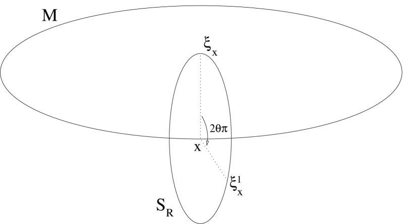
Figure 2: The $2$-torus $\mathbb{T}_{\xi}$. The $\xi_{x}^{k}$’s form a dense subset of $S_{R}$.

Similarly for any $\zeta\in{\mathbb{C}}P^{1}$ such that $z_{\xi}=z_{\zeta}$ one has $\text{Acc}(\zeta_{x})\subset\mathbb{T}_{\xi}$. In fact

$$\mathbb{T}_{\xi}=\underset{\underset{z_{\zeta}=z_{\xi}}{\zeta\in{\mathbb{C}}P^{1},}}{\bigcup}\text{Acc}(\zeta_{x}).$$ (54)

Note that when $\theta$ is irrational $\mathbb{T}_{\xi}$ is the completion of ${\text{Acc}(\xi_{x})}$ with respect to the Euclidean norm on each $S_{R}$.

Proposition V.1

$\mathbb{T}_{\xi}$ is the connected component of $\xi_{x}$ for $d$.

Proof. Let $a_{ij}\in{\cal A}_{E}$, $i,j=1,2$, be the components of a selfadjoint element of ${\cal A}$. (46) yields an explicit identification of ${\cal A}_{E}$ with the algebra of $2\pi$-periodic complex functions on ${\mathbb{R}}$,

$$a_{ij}(\tau)\doteq a_{ij}(c_{*}(\tau))=a_{ij}(\tau+2k\pi)\quad k\in{\mathbb{Z}}$$ (55)

with

$$a_{ij}(0)=a_{ij}(x).$$

Let dot denote the derivative. Since $M=S^{1}$ is $1$-dimensional, the Clifford action reduces to multiplication by $1$ ($\gamma^{\mu}=\gamma^{1}=1$) and $[D_{E},a_{ij}]=-i\dot{a_{ij}}$. Therefore

$$i[{\cal D},a]=\left(\begin{array}[]{cc}\dot{a_{11}}&\dot{a_{12}}+i\theta a_{12}\\ \dot{a_{21}}-i\theta a_{21}&\dot{a_{22}}\end{array}\right)$$ (56)

is zero if and only if $a_{11}=C$, $a_{22}=C^{\prime}$ are constant and $a_{12}=\overline{a_{21}}=0$ ($\dot{a_{12}}=-i\theta a_{12}$ has no other $2\pi$-periodic solution than zero). Under these conditions

$${\xi}_{x}(a)=\lvert V_{1}\rvert^{2}C+(1-\lvert V_{1}\rvert^{2})C^{\prime}$$

differs from ${\zeta}_{y}(a)$ if and only if $z_{\zeta}\neq z_{\xi}$. Hence, identifying $a_{ij}$ with $\underset{n\rightarrow+\infty}{\lim}(a_{n})_{ij}$ in Lemma III.2, one obtains that $d({\xi}_{x},{\zeta}_{y})$ is infinite if and only if $z_{\xi}\neq z_{\zeta}$, that is to say ${\zeta}_{y}\notin\mathbb{T}_{\xi}$. $\blacksquare$

By the proposition above the connected component $\mathbb{T}_{\xi}$ of $d$ contains, but is distinct from, the connected component $\text{Acc}(\xi_{x})$ of $d_{H}$. This is enough to establish that the two metrics are not equal. Furthermore the results of the previous section strongly suggest that even on $\text{Acc}(\xi_{x})$ the two metrics cannot coincide more than partially. To fix notation let us consider the distance $d(\xi_{x},\xi_{\tau})$ with $\xi_{\tau}\in\text{Acc}(\xi_{x})$ given by (48) with $\tau>0$. On the one hand the function on $\text{Acc}(\xi_{x})$

$$L(c(\tau))\doteq d_{H}({\xi}_{x},c(\tau))=\tau$$ (57)

is not $2\pi$-periodic, hence not in ${\cal A}_{E}$. Therefore it cannot be used as in (37) to realize the upper bound $d_{H}$ provided by Proposition III.1. Instead one could be tempted to use the geodesic distance on $S^{1}$,

$$F(\tau)\doteq d_{\text{geo}}(\xi_{x},c_{*}(\tau))=\text{min}(\tau\text{ mod }[2\pi],\;(2\pi-\tau)\text{ mod }[2\pi]),$$ (58)

but it may help in proving that $d=d_{H}$ only as long as as $d_{H}$ equals $d_{\text{geo}}$, that is to say as long as $\tau\leq\pi$. Similarly $L\text{ mod }[2\pi]$ could be efficient till $\tau=2\pi$ but it has infinite derivative at $2k\pi$ so it cannot be approximated by some $a_{n}$ satisfying the commutator norm condition. On the other hand for fixed $k\in{\mathbb{Z}}$ the projection of the minimal horizontal curve between $\xi_{\tau}^{k}$ and $\xi_{\tau}$ is a $K$-fold loop with

$$K=\left\{\begin{array}[]{lcl}\lvert k\rvert&\text{for}&\theta\text{ irrational}\\ \text{min}\{\lvert k\rvert,\lvert\lvert k\rvert-q\rvert\}&\text{for}&\theta=\frac{p}{q}\end{array}\right.$$

where we assume that $p$ and $q$ are positive relatively prime with respect to each other and $kp$ is not a multiple of $q$ (otherwise $\xi_{\tau}^{k}$ coincides with $\xi_{\tau}$). In any case when $\lvert k\rvert=1$ then $K=1$ and Proposition IV.4 should not forbid $d(\xi_{\tau},\xi_{\tau}^{\pm 1})$ from equalling $d_{H}(\xi_{\tau},\xi_{\tau}^{\pm 1})=2\pi$. We show below that this is indeed the case but only when $R=1$. On the contrary as soon as $K>3$ Proposition IV.4 certainly forbids $d$ from equalling $d_{H}$. In fact the situation is even more restrictive due to the particular choice (45) of the connection. Since the latter commutes with the diagonal part $a_{1}$ of any element $a\in{\cal A}$, $\xi_{\tau}^{k}(a_{1})=\xi_{\tau}(a_{1})$ for any $k\leq K$. Proposition IV.4 thus can be written as a system of $K+1$ equations

$$(\xi_{\tau}^{k}-\xi_{\tau})(a_{o}) = 2k\pi$$ (59)

$$\xi_{\tau}(a_{o}) = -\xi_{\tau}(a_{1})$$ (60)

where $a_{0}=a-a_{1}$. (60) simply defines the diagonal part $a_{1}$ and one is finally left with $K$ equations (59) constraining the two real components of $a_{0}$. Therefore it is most likely that $d$ does not equal $d_{H}$ as soon as $K>2$.

To make these qualitative suggestions more precise, let us study the specific example of a ”sea-level” (i.e. $z_{\xi}=0$) pure state $\xi$, assuming

$$\lvert V_{1}\rvert=\lvert V_{2}\rvert=\frac{1}{\sqrt{2}}.$$ (61)

All the distances on the associated connected component $\mathbb{T}_{\xi}$ can be explicitly computed. To do so it is convenient to isolate the part of the algebra that really enters the game in the computation of the distances. This is the objective of the following two lemmas. The first one is of algebraic nature: it deals with our explicit choice ${\cal A}_{I}=M_{2}\left({\mathbb{C}}\right)$ and does not rely on the choice $M=S^{1}$.

Lemme V.2

Given ${\zeta}_{y}$ in $\mathbb{T}_{\xi}$, the search for the supremum in the computation of $d({\xi}_{x},{\zeta}_{y})$ can be restricted to the set of elements

$$a=f{\mathbb{I}}+a_{0}$$ (62)

where ${\mathbb{I}}$ is the identity of $M_{2}\left({\mathbb{C}}\right)$, $f\in{\cal A}_{E}$ vanishes at $x$ and is positive at $y$, while $a_{0}$ is an element of ${\cal A}$ whose diagonal terms are both zero and such that

$${\zeta}_{y}(a_{0})-{\xi}_{x}(a_{0})\geq 0.$$ (63)

Proof. Let $\;\tilde{}\;$ denote the operation that permutes the elements on the diagonal. By (56)

$$\left\lVert[{\cal D},a]\right\rVert=\underset{\pm}{\max}\left\lVert\frac{(\dot{a_{11}}+\dot{a_{22}})\pm\sqrt{(\dot{a_{11}}-\dot{a_{22}})^{2}+4\lvert\dot{a_{12}}+i\theta a_{12}\rvert^{2}}}{2}\right\rVert$$ (64)

is invariant under the permutation of $a_{11}$ and $a_{22}$. Thus $\left\lVert[{\cal D},a]\right\rVert=\left\lVert[{\cal D},\tilde{a}]\right\rVert$ so

$$\left\lVert[{\cal D},\frac{\tilde{a}+a}{2}]\right\rVert\leq\left\lVert[{\cal D},a]\right\rVert.$$ (65)

Meanwhile

$${\xi}_{x}(\frac{\tilde{a}+a}{2})={\xi}_{x}(a)\;\text{ and }\;\quad{\zeta}_{y}(\frac{\tilde{a}+a}{2})={\zeta}_{y}(a)$$ (66)

therefore the supremum in the distance formula can be sought on

$${\cal A}+\tilde{{\cal A}}=C^{\infty}(S^{1})\otimes{\mathbb{I}}+{\cal A}_{0}$$

where ${\cal A}_{0}$ is the set of selfadjoint elements of ${\cal A}$ whose diagonal terms are zero. This fixes eq.(62). Now if $a=f{\mathbb{I}}+a_{0}$ attains the supremum then so does $a-f(x){\mathbb{I}}$, hence the vanishing of $f$ at $x$. Moreover

$$\left\lVert[{\cal D},f\otimes{\mathbb{I}}]\right\rVert=\left\lVert\left(\begin{array}[]{cc}1&0\\ 0&0\end{array}\right)[{\cal D},a]\left(\begin{array}[]{cc}1&0\\ 0&0\end{array}\right)\right\rVert \leq \left\lVert[{\cal D},a]\right\rVert$$ (71)

$$\left\lVert[{\cal D},a_{0}]\right\rVert\leq\left\lVert\left(\begin{array}[]{cc}0&1\\ 0&0\end{array}\right)[{\cal D},a]\left(\begin{array}[]{cc}0&1\\ 0&0\end{array}\right)\right\rVert \leq \left\lVert[{\cal D},a]\right\rVert,$$ (76)

so when $a$ satisfies the commutator norm condition so do $f{\mathbb{I}}$ and $a_{0}$. This implies that $\lvert{\xi}_{x}(a_{0})-{\zeta}_{y}(a_{0})\rvert$ and $\lvert{\xi}_{x}(f{\mathbb{I}})-{\zeta}_{y}(f{\mathbb{I}})\rvert=\lvert f(y)\rvert$ are smaller than

$$\lvert{\xi}_{x}(a)-{\zeta}_{y}(a)\rvert=\lvert f(y)+{\zeta}_{y}(a_{0})-{\xi}_{x}(a_{0})\rvert.$$ (77)

In particular, $f(y)$ and ${\zeta}_{y}(a_{0})-{\xi}_{x}(a_{0})$ have the same sign, which we assume positive (if not, consider $-a$ instead of $a$). $\blacksquare$

Other simplifications come from the choice of $S^{1}$ as the base manifold. Especially the following lemma makes clear the role played by the functions $L$ and $F$ discussed in (57,58).

Lemme V.3

Let $a=f{\mathbb{I}}+a_{0}$ satisfy the commutator norm condition, then

$$\left\lVert\dot{f}\right\rVert\leq 1\;\text{ and }\,\lvert f(\tau)\rvert\leq\left\lVert\dot{f}\right\rVert F(\tau)$$ (78)

where $F(\tau)$ is the $2\pi$-periodic function defined on $[0,2\pi[$ by

$$F(\tau)\doteq\text{min}\left(\tau,2\pi-\tau\right).$$ (79)

Meanwhile

$$a_{0}=\left(\begin{array}[]{cc}0&ge^{-i\theta L}\\ \overline{g}e^{i\theta L}&0\end{array}\right)$$ (80)

where $L(\tau)=\tau$ for all $\tau$ in ${\mathbb{R}}$ and $g$ is a smooth function on ${\mathbb{R}}$ given by

$$g(\tau)=g(0)+\int_{0}^{\tau}\rho(u)e^{i\phi(u)}du$$ (81)

with $\rho\in C^{\infty}({\mathbb{R}},{\mathbb{R}}^{+})$, $\left\lVert\rho\right\rVert\leq 1$, and $\phi\in C^{\infty}({\mathbb{R}},{\mathbb{R}})$ satisfying

$$\rho(u+2\pi)e^{i\phi(u+2\pi)}=\rho(u)e^{i(\phi(u)+2\theta\pi)}$$ (82)

while the integration constant is

$$g(0)=\frac{1}{e^{2i\theta\pi}-1}\int_{0}^{2\pi}\rho(u)e^{i\phi(u)}du.$$ (83)

Proof. (78) comes from the commutator norm condition (71) together with the $2\pi$-periodicity of $f$ (55), namely

$$f(\tau)=\int_{0}^{\tau}\dot{f}(u)du=-\int_{\tau}^{2\pi}\dot{f}(u)du.$$

The explicit form of $a_{0}$ is obtained by noting that any complex smooth function $a_{12}\in{\cal A}_{E}$ can be written $ge^{-i\theta L}$ where $g\doteq a_{12}e^{i\theta L}\in C^{\infty}({\mathbb{R}})$ satisfies

$$g(\tau+2\pi)=g(\tau)e^{2i\theta\pi}.$$ (84)

Hence any selfadjoint $a_{0}$ can be written as in (80), which yields for the commutator

$$[{\cal D},a_{0}]=-i\left(\begin{array}[]{cc}0&\dot{g}e^{-i\theta L}\\ \dot{\overline{g}}e^{i\theta L}&0\end{array}\right).$$ (85)

By (76) the commutator norm condition implies $\left\lVert\dot{g}\right\rVert\leq 1$, that is to say

$$g(\tau)=g(0)+\int_{0}^{\tau}\rho(u)e^{i\phi(u)}du$$ (86)

where $\rho\in C^{\infty}({\mathbb{R}},{\mathbb{R}}^{+})$, $\left\lVert\rho\right\rVert\leq 1$, $\phi\in C^{\infty}({\mathbb{R}},{\mathbb{R}})$. The integration constant is fixed by (84),

$$g(0)=\frac{1}{e^{2i\theta\pi}-1}\left(\int_{0}^{\tau+2\pi}\rho(u)e^{i\phi(u)}du-\int_{0}^{\tau}\rho(u)e^{i(\phi(u)+2\theta\pi)}du\right),$$ (87)

and one extracts (82) from $\frac{d}{d\tau}g(0)=0$. Reinserted in (87) it finally yields (83). $\blacksquare$

These lemmas yield the main result of the section: the computation of all distances on $\mathbb{T}_{\xi}$.

Proposition V.4

Let $P$ be the ${\mathbb{C}}P^{1}$ trivial bundle over the circle $S^{1}$ of radius one with connection (45). Let ${\xi}_{x}$ be a point in $P$ at altitude $z_{\xi}=0$ and $\mathbb{T}_{\xi}$ its connected component for the noncommutative geometry distance $d$. For any ${\zeta}_{y}\in\mathbb{T}_{\xi}$ there exists an equivalence class of real couples $(\tau,\theta^{\prime})\sim(\tau+2{\mathbb{Z}}\pi,\theta^{\prime}-2{\mathbb{Z}}\theta\pi)$ such that

$${\zeta}_{y}=\left(\begin{array}[]{cc}1&0\\ 0&e^{i\theta^{\prime}}\end{array}\right)\xi_{\tau}$$ (88)

where $\xi_{\tau}$ is given in (48,47). Without loss of generality one may assume that $\tau$ is positive (if not, permute the role played by ${\xi}_{x}$ and ${\zeta}_{y}$) so that

$$\tau=2k\pi+\tau_{0}$$ (89)

with $k\in{\mathbb{N}}$ and $0\leq\tau_{0}\leq 2\pi$. Then

$$d({\xi}_{x},{\zeta}_{y})=\left\{\begin{array}[]{ll}\max\left(\,X;X+\tau_{0}Y\,\right)&\text{when }\tau_{0}\leq\pi\\ \max\left(\,X;X+(2\pi-\tau_{0})Y\,\right)&\text{when }\pi\leq\tau_{0}\end{array}\right.$$ (90)

in which

$$X \doteq RW_{k+1}\tau_{0}+RW_{k}(2\pi-\tau_{0})$$ (91)

$$Y \doteq 1-RW_{k+1}-RW_{k}$$ (92)

with $R$ defined in (50) and

$$W_{k}\doteq\frac{\lvert\sin(k\theta\pi+\frac{\theta^{\prime}}{2})\rvert}{\lvert\sin\theta\pi\rvert}$$ (93)

do not depend on the choice of the representantive of the equivalence class $(\tau,\theta^{\prime})$.

Proof. The form (88) of ${\zeta}_{y}$ comes from the definition (54) of $\mathbb{T}_{\xi}$. It gives, for an element $a$ of Lemma V.3,

$$\lvert{\xi}_{x}(a)-{\zeta}_{y}(a)\rvert=f(\tau)+\Re\left(Re^{-i\theta_{0}}(g(\tau)e^{i\theta^{\prime}}-g(0))\right)$$ (94)

where we use the definition (50) of $\theta_{0}$, the vanishing of $f$ at $x$, the positivity of $f(y)=f(\tau)$ as well as (63). The explicit form (81) of $g$ allows us to rewrite (94) as

$$f(\tau)+R\int_{0}^{\tau}\rho(u)\cos(\phi^{\prime}(u))+\Re\left(Re^{-i\theta_{0}}g(0)\left(e^{i\theta^{\prime}}-1\right)\right)$$ (95)

where

$$\phi^{\prime}(u)\doteq\phi(u)-\theta_{0}+\theta^{\prime}.$$

The point is to find the maximum of (95) on all the $2\pi$-periodic $f$ satisfying (78), the positive $\rho$, $\left\lVert\rho\right\rVert\leq 1$ and the $\phi$ satisfying (82). To do so we will first find an upper bound (eqs. (113) and (114) below) and prove that it is the lowest one.

Fixing a pure state ${\zeta}_{y}$ means fixing two values $\theta^{\prime}$ and $\tau$ or, equivalently by (89), fixing $\theta^{\prime}$, $k$ and $\tau_{0}$. The integral term in (95) then splits into

$$\Re\int_{0}^{2k\pi}\rho(u)e^{i\phi^{\prime}(u)}du=\Re\left(\underset{n=0}{\overset{k-1}{\Sigma}}e^{2in\theta\pi}\int_{0}^{2\pi}\rho(u)e^{i\phi^{\prime}(u)}du\right)$$ (96)

and

$$\Re\int_{2k\pi}^{2k\pi+\tau_{0}}\rho(u)e^{i(\phi^{\prime}(u)})du=\Re\left(e^{2ik\theta\pi}\int_{0}^{\tau_{0}}\rho(u)e^{i\phi^{\prime}(u)}du\right)$$ (97)

that recombine as

$$S_{k+1}\int_{0}^{\tau_{0}}\rho(u)\cos\phi_{k}(u)\,du+S_{k}\int_{\tau_{0}}^{2\pi}\rho(u)\cos\phi_{k_{1}}(u)\,du$$ (98)

where

$$S_{k}\doteq\frac{\sin k\theta\pi}{\sin\theta\pi}\,\text{ and }\,\phi_{k}(u)\doteq\phi^{\prime}(u)+k\theta\pi.$$ (99)

To compute the real-part term of (95) one uses the definition (83) of $g(0)$ and obtain

$$S_{\frac{1}{2}}\int_{0}^{2\pi}\rho(u)\cos\phi_{\frac{1}{2}}(u)\,du$$ (100)

where

$$S_{\frac{1}{2}}\doteq\frac{\sin\theta^{\prime}/2}{\sin\theta\pi}\,\text{ and }\,\phi_{1/2}(u)\doteq\phi^{\prime}(u)-\frac{\theta^{\prime}}{2}-\theta\pi.$$

(95) is rewritten as

$$\lvert{\xi}_{x}(a)-{\zeta}_{y}(a)\rvert=f(\tau)+R\int_{0}^{\tau_{0}}\rho(u)G_{k+1}(u)\,du+R\int_{\tau_{0}}^{2\pi}\rho(u)G_{k}(u)\,du$$ (101)

with

$$G_{k}\doteq S_{k}\cos\phi_{k-1}+S_{\frac{1}{2}}\cos\phi_{\frac{1}{2}}.$$ (102)

The split of the integral makes the search for the lowest upper bound easier. Calling $W_{k}$ the maximum of $\lvert G_{k}(u)\rvert$ on $[0,2\pi[$, the positivity of $\rho$ makes (101) bounded by

$$f(\tau)+RW_{k+1}\int_{0}^{\tau_{0}}\rho(u)\,du+RW_{k}\int_{\tau_{0}}^{2\pi}\rho(u)\,du.$$ (103)

Now (64) with $a_{11}=a_{22}=f$ and $\lvert\dot{a_{21}}+i\theta a_{12}\rvert=\rho$ yields

$$\lvert\dot{f}(u)+\rho(u)\rvert\leq 1 \lvert\dot{f}(u)\rvert\geq 0$$ whenever (104)

$$\lvert\dot{f}(u)-\rho(u)\rvert\leq 1 \lvert\dot{f}(u)\rvert\leq 0$$ whenever (105)

for any $u\in{\mathbb{R}}$, that is to say

$$\rho\leq 1-\lvert\dot{f}\rvert.$$ (106)

Therefore

$$\int_{0}^{\tau_{0}}\rho(u)\,du\leq\tau_{0}-\int_{0}^{\tau_{0}}\lvert\dot{f}\rvert.$$ (107)

Moreover $f(\tau)=f(\tau_{0})$ ($2\pi$-periodicity of $f$) is positive by Lemma V.2 so

$$-f(\tau_{0})=-\lvert f(\tau_{0})\rvert\geq-\int_{0}^{\tau_{0}}\lvert\dot{f}(u)\rvert\,du.$$ (108)

Hence (107) gives

$$\int_{0}^{\tau_{0}}\rho(u)\,du\leq\tau_{0}-f(\tau_{0}).$$ (109)

Similarly

$$\int_{\tau_{0}}^{2\pi}\lvert\dot{f}(u)\rvert du\geq\lvert\int_{\tau_{0}}^{2\pi}\dot{f}(u)du\rvert=\lvert-\int_{0}^{\tau_{0}}\dot{f}(u)\,du\rvert=f(\tau_{0})$$

hence

$$\int_{\tau_{0}}^{2\pi}\rho(u)\,du\leq 2\pi-\tau_{0}-f(\tau_{0}).$$ (110)

Back to (103), equations (109) and (110) yield the bound

$$f(\tau_{0})Y+X$$ (111)

where $X$ is defined in (91) and $Y$ in (92). By (78) and in case

$$Y\geq 0,$$ (112)

(111) yields

$$\lvert{\xi}_{x}(a)-{\zeta}_{y}(a)\rvert\leq\left\{\begin{array}[]{ll}X+\tau_{0}Y&\text{for }0\leq\tau_{0}\leq\pi\\ X+(2\pi-\tau_{0})Y&\text{for }\pi\leq\tau_{0}\leq 2\pi\end{array}\right..$$ (113)

When $Y\leq 0$,

$$\lvert{\xi}_{x}(a)-{\zeta}_{y}(a)\rvert\leq X.$$ (114)

These are the announced lowest upper bounds. To convince ourselves let us build a sequence $a_{n}$ that realizes (113) or (114) at the limit $n\rightarrow+\infty$. As a preliminary step note that an easy calculation from (102) yields

$$G_{k}=A_{k}\cos\phi^{\prime}+B_{k}\sin\phi^{\prime}$$

where

$$A_{k} \doteq S_{\frac{1}{2}}\cos(\frac{\theta^{\prime}}{2}+\theta\pi)+S_{k}\cos(k-1)\theta\pi$$ (115)

$$B_{k} \doteq S_{\frac{1}{2}}\sin(\frac{\theta^{\prime}}{2}+\theta\pi)-S_{k}\sin(k-1)\theta\pi.$$ (116)

$G_{k}$ attains its maximum value

$$W_{k}\doteq\lvert A_{k}\rvert\sqrt{1+\frac{\lvert B_{k}\rvert^{2}}{\lvert A_{k}\rvert^{2}}}=\frac{\lvert\sin(k\theta\pi+\frac{\theta^{\prime}}{2})\rvert}{\lvert\sin(\theta\pi)\rvert}$$ (117)

when

$$\phi^{\prime}=\Phi_{k}\doteq\text{Arctan}\frac{B_{k}}{A_{k}}\,\text{ or }\,\text{Arctan}\frac{B_{k}}{A_{k}}+\pi.$$ (118)

Let then

$$a_{n}=\left(\begin{array}[]{cc}f_{n}&g_{n}e^{-i\theta L}\\ \overline{g}_{n}e^{i\theta L}&f_{n}\end{array}\right)$$

be a sequence of elements of ${\cal A}$ that depend on the fixed value $\tau=2k\pi+\tau_{0}$ in the following way: in case (112) is fulfilled and $\tau_{0}\leq\pi$, $f_{n}$ approximates from below the $2\pi$-periodic function

$$f_{-}(t)=\left\{\begin{array}[]{ll}t&\text{ for }\,0\leq t\leq\tau_{0}\\ \tau_{0}-C(t-\tau_{0})&\text{ for }\,\tau_{0}\leq t\leq 2\pi\end{array}\right.$$ (119)

with

$$C\doteq\frac{\tau_{0}}{2\pi-\tau_{0}}.$$

In case $\tau_{0}\geq\pi$, $f_{n}$ approximates

$$f_{+}(t)=\left\{\begin{array}[]{ll}\frac{t}{C}&\text{ for }\,0\leq t\leq\tau_{0}\\ 2\pi-t&\text{ for }\,\tau_{0}\leq t\leq 2\pi\end{array}\right..$$ (120)

Figure 3: The functions $F$, $f_{+}$ and $f_{-}$.

When (112) is not fulfilled, $f_{n}=f_{0}$ is simply the zero function. In any case and whatever $\tau_{0}$, $g_{n}$ is defined via (81) and (83), replacing $\phi$ with a sequence $\phi_{n}$ approximating the step function $\Phi$ of width $2\pi$ and height $2\theta\pi$ defined on $[0,2\pi[$ by

$$\Phi(u)=\left\{\begin{array}[]{ll}\Phi_{k+1}+\theta_{0}-\theta^{\prime}&\text{ for }0\leq u<\tau_{0}\\ \Phi_{k}+\theta_{0}-\theta^{\prime}&\text{ for }\tau_{0}<u<\pi\end{array}\right.,$$ (121)

and replacing $\rho$ with a sequence $\rho_{n}$ approximating the $2\pi$-periodic function

$$\Gamma_{I}=1-\lvert\dot{f_{I}}\rvert$$ (122)

where $I=+,-$ or $0$. By construction the $a_{n}$’s satisfy the commutator norm condition. In particular the fact that $\underset{n\rightarrow+\infty}{\text{lim}}\rho_{n}$ and $\Phi$ are step functions is not problematic since their derivatives are not constrained by the commutator. For technical details on how to approximate step functions by sequences of smooth functions, the reader is invited to consult classical textbooks such as [?]. The last point is to check that

$$\underset{n\rightarrow+\infty}{\text{lim}}\lvert{\xi}_{x}(a_{n})-{\zeta}_{y}(a_{n})\rvert=(\ref{boundfinal}).$$ (123)

This is a simple notation exercise: (99) gives

$$\phi^{\prime}(u) = \Phi_{k+1}\;\text{ for }\,0\leq u<\tau_{0}$$ (124)

$$\phi^{\prime}(u) = \Phi_{k}\quad\text{ for }\,\tau_{0}<u<2\pi.$$ (125)

Therefore, by (101) together with (122),

$$\underset{n\rightarrow+\infty}{\text{lim}}\lvert{\xi}_{x}(a_{n})-{\zeta}_{y}(a_{n})\rvert = f_{I}(\tau_{0})+RW_{k+1}\int_{0}^{\tau_{0}}\Gamma_{I}(u)\,du+RW_{k}\int_{\tau_{0}}^{2\pi}\Gamma_{I}(u)\,du$$ (126)

$$= f_{I}(\tau_{0})-RW_{k+1}\int_{0}^{\tau_{0}}\lvert\dot{f_{\pm}}\rvert\,du-RW_{k}\int_{\tau_{0}}^{2\pi}\lvert\dot{f_{I}}\rvert\,du$$

$$+RW_{k+1}\tau_{0}+RW_{k}(2\pi-\tau_{0}).$$

When $(\ref{condfinale})$ is fulfilled and $\tau_{0}\leq\pi$, the subscript of $f$ is minus and (119) makes (126) equal to

$$\tau_{0}-RW_{k+1}\tau_{0}-RW_{k}(2\pi-\tau_{0})C+RW_{k+1}\tau_{0}+RW_{k}(2\pi-\tau_{0})$$

which is exactly the first line of (113). Similarly for $\tau_{0}\geq\pi$, the subscript turns to $+$ and (120) yields for (126)

$$(2\pi-\tau_{0})-RW_{k+1}\frac{\tau_{0}}{C}-RW_{k}(2\pi-\tau_{0})+RW_{k+1}\tau_{0}+RW_{k}(2\pi-\tau_{0}),$$

which is nothing but the second line of (113). Finally, when (112) is not fulfilled, $f_{I}=\dot{f}_{I}=0$ and (126) equals (114). $\blacksquare$

Let us check the coherence of our result by noticing that for $\tau_{0}=\pi$ both formulas of (90) agree and yield

Check 1

$d({\xi}_{x},\zeta_{\pi})=\max\left(X,X+\pi Y\right)=\max\left(\pi R(W_{k+1}+W_{k});\,\pi\right).$

Similarly for a given $k$ and $\tau_{0}=2\pi$, the second line of (90) agrees with the first line with $k+1$ and $\tau_{0}=0$, namely

Check 2

$d({\xi}_{x},\zeta_{2k\pi+2\pi})=2\pi RW_{k+1}=d({\xi}_{x},\zeta_{2(k+1)\pi+0}).$

This is nothing but the restriction of $d$ to the fiber over $x$. Its extreme simplicity (no ”max” is involved) indicates that the noncommutative metric is better understood fiberwise. We shall see in the next section that this is the main difference from the Carnot-Carathéodory metric. Another check, and certainly the best guarantee that Proposition V.4 is true, is to directly verify that formula (90) does define a metric: the vanishing of $d$ when ${\zeta}_{y}={\xi}_{x}$ is obvious; the invariance under the exchange ${\xi}_{x}\longleftrightarrow{\zeta}_{y}$ is not testable since the symmetry $\tau\longleftrightarrow-\tau$ is broken from the beginning by the specification that $\tau$ is positive. There remains the triangle inequality.

Check 3

For any $\zeta_{1},\zeta_{2}\in\mathbb{T}_{\xi}$, $d(\xi_{x},\zeta_{2})\leq d(\xi_{x},\zeta_{1})+d(\zeta_{1},\zeta_{2}).$

Proof. Let $\zeta_{\tau_{i}}$, $i=1,2$, be two pure states defined by $\tau_{i}=2\pi k_{i}+t_{i}$ and $\theta^{\prime}_{i}$, labeled in such a way that $\tau_{1}\leq\tau_{2}$. The point is to check that

$$\Delta\doteq d({\xi}_{x},\zeta_{\tau_{1}})+d(\zeta_{\tau_{1}},\zeta_{\tau_{2}})-d({\xi}_{x},\zeta_{\tau_{2}})$$ (127)

is positive. Proposition V.4 is invariant under translation (i.e. a reparameterization of the circle $\tau\rightarrow\tau+\text{constant}$), which means that $d(\zeta_{\tau_{1}},\zeta_{\tau_{2}})$ is given by formula (90) with $W_{k}$ replaced by

$$W_{k_{12}}\doteq\frac{\lvert\sin(k_{12}\theta\pi+\frac{\theta^{\prime}_{2}-\theta^{\prime}_{1}}{2})\rvert}{\lvert\sin\theta\pi\rvert}$$

and $\tau_{0}$ replaced by $t_{12}$. Here $k_{12}$ and $t_{12}$ are such that $\tau_{12}\doteq\tau_{2}-\tau_{1}\doteq 2k_{12}\pi+t_{12}$. Explicitly

$$k_{12}=k_{2}-k_{1}, \;t_{12}=t_{2}-t_{1} \text{ if }\,t_{1}\leq t_{2}$$ (128)

$$k_{12}=k_{2}-k_{1}-1, \;t_{12}=2\pi+t_{2}-t_{1} \text{ if }\,t_{2}\leq t_{1}.$$ (129)

Let $X_{i},Y_{i}$, $i\in\{1,2,12\},$ denote (91) and (92) in which $k$ is replaced by $k_{i}$. The only difficulty in checking that (127) is positive is the quite large number of possible expressions for $\Delta$: one for each combination of the signs of the $Y_{i}$’s and $t_{i}-\pi$. A simple way to reduce the number of cases under investigation is to decorate $\Delta$ with three arrows indicating whether $Y_{1}$, $Y_{12}$ and $Y_{2}$ respectively are positive (upper arrow) or negative (lower arrow). For instance $\Delta_{\uparrow\uparrow\downarrow}$ denotes the value of $\Delta$ when $Y_{1}\geq 0$, $Y_{12}\geq 0$, and $Y_{2}\leq 0$. Let us also use $\tilde{\Delta}$ decorated with arrows to denote the formal expression (127) in which $d({\xi}_{x},\xi_{\tau_{1}})$, $d(\zeta_{\tau_{1}},\zeta_{\tau_{2}})$ and $d({\xi}_{x},\zeta_{\tau_{2}})$ are replaced either by $X_{i}+t_{i}^{m}Y_{i}$ (upper arrow) or by $X_{i}$ (lower arrow). Here $t_{i}^{m}\doteq\min\left(t_{i},2\pi-t_{i}\right)$. For instance

$$\tilde{\Delta}_{\uparrow\uparrow\uparrow} = \tilde{\Delta}_{\downarrow\uparrow\uparrow}+t_{1}^{m}Y_{1}$$ (130)

$$= \tilde{\Delta}_{\uparrow\downarrow\uparrow}+t_{2}^{m}Y_{2}$$ (131)

$$= \tilde{\Delta}_{\downarrow\downarrow\uparrow}+t_{1}^{m}Y_{1}+t_{2}^{m}Y_{2}.$$ (132)

Now suppose that $Y_{1}$, $Y_{12}$, $Y_{2}$ are all positive, then

$$\Delta=\Delta_{\uparrow\uparrow\uparrow}=\tilde{\Delta}_{\uparrow\uparrow\uparrow}\geq\left\{\begin{array}[]{c}\tilde{\Delta}_{\downarrow\uparrow\uparrow}\\ \tilde{\Delta}_{\uparrow\downarrow\uparrow}\\ \tilde{\Delta}_{\downarrow\downarrow\uparrow}\end{array}\right..$$

Changing the sign of $Y_{1}\leq 0$ and $Y_{12}$ yields

$$\Delta=\Delta_{\downarrow\downarrow\uparrow}=\tilde{\Delta}_{\downarrow\downarrow\uparrow}\geq\left\{\begin{array}[]{c}\tilde{\Delta}_{\uparrow\downarrow\uparrow}\\ \tilde{\Delta}_{\downarrow\uparrow\uparrow}\\ \tilde{\Delta}_{\uparrow\uparrow\uparrow}\end{array}\right..$$

Therefore, if one is able to show without using the sign of $Y_{1}$ or the sign of $Y_{12}$ that $\tilde{\Delta}_{\uparrow\uparrow\uparrow}$ is positive, one proves that both $\Delta_{\uparrow\uparrow\uparrow}$ and $\Delta_{\downarrow\downarrow\uparrow}$ are positive. In fact showing that one of the $\tilde{\Delta}_{\updownarrow\updownarrow\uparrow}$’s is positive is enough to prove that all the $\Delta_{\updownarrow\updownarrow\uparrow}$’s are positive (here $\updownarrow$ means either $\uparrow$ or $\downarrow$). Of course the same is true with $\tilde{\Delta}_{\updownarrow\updownarrow\downarrow}$ so that, at the end, one just has to check the inequality of the triangle for one of the $\tilde{\Delta}_{\updownarrow\updownarrow\uparrow}$ and one of the $\tilde{\Delta}_{\updownarrow\updownarrow\downarrow}$.

Let us begin by $\tilde{\Delta}_{\updownarrow\updownarrow\downarrow}$, assuming first $t_{1}\leq t_{2}$. With $W_{i}\doteq W_{k_{i}}$, $W_{i+1}\doteq W_{k_{i}+1}$, (128) yields

$$R^{-1}\tilde{\Delta}_{\downarrow\downarrow\downarrow} = W_{1+1}t_{1}+W_{1}(2\pi-t_{1})+W_{12+1}t_{12}+W_{12}(2\pi-t_{12})$$

$$-W_{2+1}t_{2}-W_{2}(2\pi-t_{2})$$

$$= (2\pi-t_{2})(W_{1}+W_{{12}}-W_{2})+t_{12}(W_{1}+W_{{12}+1}-W_{2+1})$$

$$+t_{1}(W_{1+1}+W_{{12}}-W_{2+1})$$

which is positive since

$${W_{k_{2}}}\leq{W_{k_{1}}}+{W_{k_{12}}}$$ (133)

and similar equations for the other indices. Assuming now $t_{2}\leq t_{1}$, (129) yields

$$R^{-1}\tilde{\Delta}_{\downarrow\downarrow\downarrow} = t_{2}(W_{1+1}+W_{12+1}-W_{2+1})+(2\pi-t_{1})(W_{1}+W_{12+1}-W_{2})$$

$$+(2\pi-t_{12})(W_{12}+W_{1+1}-W_{2})$$

which is also positive by equations similar to (133) (be careful to use the definition (129) of $k_{12}$ and no longer definition (128)). Thus, whatever $t_{1}$ and $t_{2}$, $\tilde{\Delta}_{\updownarrow\updownarrow\downarrow}$ is positive and the triangle inequality is checked for all the configurations $\updownarrow\updownarrow\downarrow$ of the $Y_{i}$’s.

Things are slightly more complicated for the configurations $\updownarrow\updownarrow\uparrow$ for one also has to deal with the signs of $t_{i}-\pi$. First assume $t_{1}\leq t_{2}$:

• $\ t_{1}\leq t_{2}\leq\pi$ (implies $t_{12}\leq\pi$),

  $$(2R)^{-1}\tilde{\Delta}_{\uparrow\uparrow\uparrow} = {W_{1}}(\pi-t_{1})+{W_{{12}}}(\pi-t_{12})-{W_{2}}(\pi-t_{2})$$

  $$\geq (\pi-t_{2})({W_{1}}+{W_{{12}}}-W_{2}).$$

• $\pi\leq\ t_{1}\leq t_{2}$ (implies $t_{12}\leq\pi$),

  $$\tilde{\Delta}_{\uparrow\uparrow\uparrow} = 2R(W_{1+1}(t_{1}-\pi)+W_{{12}}(\pi-t_{12})-W_{2+1}(t_{2}-\pi))+2(t_{2}-t_{1})$$

  $$\geq 2R(t_{1}-\pi)(W_{1+1}+W_{{12}}-W_{2+1})+2(t_{2}-t_{1})(1-RW_{2+1}).$$

• $t_{1}\leq\pi\leq t_{2}$ and $t_{12}\leq\pi$,

  $$\tilde{\Delta}_{\uparrow\uparrow\uparrow}=2R(W_{1}(\pi-t_{1})+W_{{12}}(\pi-t_{12}))+2(t_{2}-\pi)(1-RW_{2+1}).$$

• $t_{1}\leq\pi\leq t_{2}$ and $t_{12}\geq\pi$,

  $$\tilde{\Delta}_{\uparrow\uparrow\uparrow} = 2R(W_{1}(\pi-t_{1})+W_{{12}+1}(t_{12}-\pi)-W_{{2}+1}(t_{12}-\pi))+t_{1}(1-2RW_{{2}+1})$$

  $$\geq 2R(t_{12}-\pi)(W_{1}+W_{{12}+1}-W_{{2}+1})+2t_{1}(1-RW_{{2}+1}).$$

These five expressions are positive by (133) and the positivity of $Y_{2}$. Similarly, in case $t_{2}\leq t_{1}$:

• $t_{2}\leq t_{1}\leq\pi$ (implies $t_{12}\geq\pi$),

  $$\tilde{\Delta}_{\uparrow\uparrow\uparrow} = 2R(W_{1}(\pi-t_{1})+W_{{12}+1}(t_{12}-\pi)-W_{2}(\pi-t_{1}))+2(t_{1}-t_{2})(1-R{W_{2}})$$

  $$\geq 2R(\pi-t_{1})\left(W_{1}+W_{{12}+1}-W_{2}\right)+2(t_{1}-t_{2})\left(1-R{W_{2}}\right).$$

• $\pi\leq\ t_{2}\leq t_{1}$ (implies $t_{12}\geq\pi$),

  $$(2R)^{-1}\tilde{\Delta}_{\uparrow\uparrow\uparrow} = W_{1+1}(t_{1}-\pi)+W_{{12}+1}(t_{12}-\pi)-W_{2+1}(t_{2}-\pi)$$

  $$\geq (t_{2}-\pi)(W_{1+1}+W_{{12}+1}-W_{2+1}).$$

• $t_{2}\leq\pi\leq t_{1}$ and $t_{12}\leq\pi$,

  $$\tilde{\Delta}_{\uparrow\uparrow\uparrow} = 2R(W_{1+1}(t_{1}-\pi)+W_{{12}}(\pi-t_{12})-W_{2}(\pi-t_{12}))+2(2\pi-t_{1})(1-RW_{2})$$

  $$\geq 2R(\pi-t_{12})(W_{1+1}+W_{{12}}-W_{2})+2(2\pi-t_{1})(1-RW_{2}).$$

• $t_{2}\leq\pi\leq t_{1}$ and $t_{12}\geq\pi$,

  $$\tilde{\Delta}_{\uparrow\uparrow\uparrow} = 2RW_{1+1}(t_{1}-\pi)+2RW_{{12}+1}(t_{12}-\pi)+2(\pi-t_{2})(1-RW_{2}).$$

  $\blacksquare$

The proof above is long but we believe it is important to convince oneself that formula V.4 does define a metric, which is not obvious at first sight. As a final test, let us come back to the beginning of this section and verify Lemma III.1.

Check 4

$d({\xi}_{x},{\zeta}_{y})\leq d_{H}({\xi}_{x},{\zeta}_{y})\,\text{ for any }\,{\zeta}_{y}\in\text{Acc}({\xi}_{x}).$

Proof. Let ${\zeta}_{y}=\xi_{\tau}$. Then $d_{H}({\xi}_{x},\xi_{\tau})=2k\pi+\tau_{0}$ so that

$$d({\xi}_{x},\xi_{\tau})-d_{H}({\xi}_{x},\xi_{\tau})\left\{\begin{array}[]{lll}=&2RW_{k}(\pi-\tau_{0})-2k\pi&\\ &\leq 2\pi(W_{k}-k)&\text{ when }Y\geq 0,\,\tau_{0}\leq\pi,\\ =&2RW_{k+1}(\tau_{0}-\pi)-2(\tau_{0}-\pi)-2k\pi&\\ &\leq-2(\tau_{0}-\pi)W_{k}-2k\pi&\text{ when }Y\geq 0,\,\tau_{0}\geq\pi,\\ =&\tau_{0}(RW_{k+1}-RW_{k}-1)\\ &+2\pi(RW_{k}-k)&\text{ when }Y\leq 0.\end{array}\right.$$ (134)

These three expressions are negative by (133) and $\lvert\sin k\theta\pi\rvert\leq k\lvert\sin\theta\pi\rvert.$ $\blacksquare$

Figure 4: $d({\xi}_{x},\xi_{\tau})\,$ as a function of $\tau$ for $\theta=\frac{1}{\sqrt{2}}$, $R=0.75$. The dashed line is $d_{H}({\xi}_{x},\xi_{\tau})$. The unit is $\pi$.

VI Interpretation: a smooth cardio-torus

This section aims at analyzing the result of Proposition V.4. We first compare $d$ to $d_{H}$ on $\text{Acc}({\xi}_{x})$ (corollaries VI.1 and VI.2), then study the restriction of $d$ to the fiber over $x$ and to the base $M=S^{1}$. The reader may wonder why we do not systematically replace $R$ by its value $1$. The point is that for two states on the same fiber ($y=x$) the diagonal part of $a$ does not play any role so that Proposition V.4 is valid also for non vanishing $z_{\xi}$. Also, for $y\neq x$ some calculations^? show that V.4 is still valid for non-zero $z_{\xi}$ as long as $2V^{2}_{i}-R(W_{k+1}+W_{k})$ is positive for both $i=1,2$. This is the reason why, in the following discussion, we keep writing $R$.

VI.1 The shape of $\mathbb{T}_{\xi}$

Taking ${\zeta}_{y}$ in $\text{Acc}({\xi}_{x})$ amounts to setting $\theta^{\prime}=0$. $W_{k}$ is replaced by

$$S_{k}\doteq\frac{\lvert\sin k\theta\pi\rvert}{\lvert\sin\theta\pi\rvert}$$

and proposition V.4 is rewritten in a somehow more readable fashion.

Corollary VI.1

Let ${\zeta}_{y}=\xi_{\tau}\in\text{Acc}({\xi}_{x})$, with $\tau=2k\pi+\tau_{0}.$ For $k$ such that $S_{k+1}+S_{k}\leq\frac{1}{R}$,

$$d({\xi}_{x},\xi_{\tau})=\left\{\begin{array}[]{ll}\displaystyle 2RS_{k}(\pi-\tau_{0})+\tau_{0}&\text{when }\tau_{0}\leq\pi\\ 2RS_{k+1}(\tau_{0}-\pi)+2\pi-\tau_{0}&\text{when }\pi\leq\tau_{0}\end{array}\right..$$ (135)

For $k$ such that $S_{k+1}+S_{k}\geq\frac{1}{R}$,

$$d({\xi}_{x},\xi_{\tau})=RS_{k+1}\tau_{0}+RS_{k}(2\pi-\tau_{0}).$$

It is easy to see on which part of $P$ the noncommutative geometry metric and the Carnot-Carathéodory one coincide.

Corollary VI.2

For any $R$, $d({\xi}_{x},\xi_{\tau})=d_{H}({\xi}_{x},\xi_{\tau})$ for $\tau\in[0,\pi]$. Moreover if $R=1$ the two metrics are also equal for $\tau\in[\pi,2\pi]$. These are the only situations in which $d=d_{H}$.

Proof. $S_{0}=0$, $S_{1}=1$ and by construction $R\leq 1$. Therefore for $k=0$, $S_{k+1}+S_{k}=1\leq\frac{1}{R}$ so

$$d({\xi}_{x},\xi_{\tau})=\left\{\begin{array}[]{ll}\displaystyle\tau_{0}=d_{H}({\xi}_{x},\xi_{\tau_{0}})&\text{when }\tau_{0}\leq\pi\\ 2\pi(1-R)+\tau_{0}(2R-1)&\text{when }\pi\leq\tau_{0}\end{array}\right.$$ (136)

which yields the equality of $d$ and $d_{H}$ for the indicated values of $\tau$ and $R$. From check 4 in the preceding section, $d$ may equal $d_{H}$ only if $S_{k}=k$, i.e. $k=0$ or $1$. When $k=1$, $S_{k}+S_{k+1}\geq 1$ and the last line of (134) gives the difference $\delta$ between $d$ and $d_{H}$,

$$\delta=\tau_{0}(RS_{2}-R-1)+2\pi(R-1).$$ (137)

$S_{2}\leq 2$ so $\delta\leq(R-1)(2\pi+\tau)$. $\delta$ may vanish only if $R=1$ and, going back to (137), only if $\tau_{0}=0$. $\blacksquare$

This result is more restrictive that what was expected from Proposition IV.4 revisited in (59), namely that $d$ may equal $d_{H}$ as long as $c$ does not have sequences of more than $2$ self-intersecting points, i.e. up to $\tau_{\text{max}}=4\pi+\tau_{0}$. It seems that Proposition IV.4 alone is not sufficient to show that $\tau_{\text{max}}\leq 2\pi$. At best one can obtain

$$\tau_{\text{max}}<4\pi.$$ (138)

Although (138) is not in se an interesting result but simply a weaker formulation of Corollary VI.2, we believe it is interesting to see how far Proposition IV.4 can lead. This could be the starting point for a generalization of the results of this paper to manifolds other than $S^{1}$. Let $G,\overline{G}$ be the off-diagonal components of $a$. (59) is rewritten as

$$\Im\left(G(\tau)e^{i(\theta\tau-\theta_{0})}e^{ik\theta\pi}\right)=-\frac{k\pi}{R\sin k\theta\pi}$$ (139)

for any $k=1,...,K$. For $K=2$ this system has a unique solution

$$G(\tau)=Ce^{-i\theta\tau}e^{i(\theta_{0}-\frac{\pi}{2})}$$ (140)

where

$$C\doteq-\frac{2\pi}{R\sin 2\theta\pi}$$

is a constant. Therefore $\xi_{\tau}(a_{0})=\Re\left(e^{i(\theta\tau-\theta_{0})}G(\tau)\right)=0$ so that, by (60), $\xi_{\tau}(a)=0$. By Proposition IV.4 this is possible only for $\tau=0$. Hence there cannot be more than one sequence of 2 self-intersecting points, hence (138).

In any case, when $\tau$ is greater than $2\pi$, $d$ strongly differs from $d_{H}$. While the latter is unbounded, the former is bounded,

$$d({\xi}_{x},{\zeta}_{y})\leq\text{max}(\frac{2\pi R}{\lvert\sin\theta\pi\rvert},\pi).$$

As illustrated in figure 4, $\text{Acc}({\xi}_{x})$ viewed as a $1$-dimensional object looks like a straight line when it is equipped with $d_{H}$, whereas it looks rather chaotic when it is equipped with $d$.

VI.2 The shape of the fiber

From a fiberwise point of view the situation drastically changes. Parameterizing the fiber $S_{x}$ over $x$ by

$$\phi\doteq 2k\theta\pi+\theta^{\prime}\text{ mod }[2\pi],$$

one obtains a very simple expression for the noncommutative distance,

$$d(0,\phi)=\frac{2\pi R}{\lvert\sin\theta\pi\rvert}\sin\frac{\phi}{2}.$$ (141)

For those points of $S_{x}$ which are accessible from ${\xi}_{x}$, namely for $\theta^{\prime}=0$, the Carnot-Carathéodory metric is

$$d_{H}(0,\phi)=2k\pi.$$

Hence, when $\theta$ is irrational and in any neighborhood of ${\xi}_{x}=0$ in the Euclidean topology of $S_{x}$, it is always possible to find some

$$\phi_{k}\doteq\xi_{0}^{k}=2k\theta\pi\text{ mod }[2\pi]$$

which are arbitrarily Carnot-Carathéodory-far from ${\xi}_{x}$. In other terms $d_{H}$ destroys the $S^{1}$ structure of the fiber. On the contrary $d$ keeps it in mind in a rather intriguing way. Let us compare $d$ to the Euclidean distance $d_{E}$ on the circle of radius

$$\mathcal{R}\doteq\frac{2R}{\lvert\sin\theta\pi\rvert}.$$ (142)

At the cut-locus $\phi=\pi$, the two distances are equal but whereas $d_{E}(0,.)$ is not smooth, the noncommutative geometry distance is smooth (cf Figure 5).

Figure 5: $d_{H}(0,\phi_{k})$, $d(0,\phi_{k})$, $d_{E}(0,\phi_{k})$. Vertical unit is $\frac{\pi R}{\sin\theta\pi}$, horizontal unit is $\pi$.

In this sense, if we imagine an observer localized at ${\xi}_{x}$ and whose only information about the geometry of the surrounding world is the measurement of the function $d(0,\phi)$, $S_{x}$ looks ”smoother than a circle”. More rigourously, (141) turns out to be the length $L(\phi)$ of the minimal arc joining the origin to a point $\phi$ on the cardioid with polar equation

$$r=\frac{\pi\mathcal{R}}{4}(1+\cos\varphi).$$ (143)

Figure 6: Cardioid $r=\frac{\pi\mathcal{R}}{4}(1+\cos\varphi)$. Units are in $\frac{\pi R}{\lvert\sin\theta\pi\rvert}$.

Indeed restricting to $0\leq\phi\leq\pi$ (since $L(\phi)=L(2\pi-\phi)$),

$$L(\phi)=\int_{0}^{\phi}\sqrt{r^{2}+(\frac{dr}{d\varphi})^{2}}d\varphi=\int_{0}^{\phi}\frac{\pi\mathcal{R}}{2}\cos\frac{\varphi}{2}d\varphi=\pi\mathcal{R}\sin\frac{\phi}{2}=d(0,\phi).$$ (144)

One has to be careful with the interpretation of equation (144). The noncommutative geometry distance does not turn the loop $S_{x}$ into a cardioid. What the noncommutative metric does is to turn $S_{x}$ into an object that looks like a cardioid for an observer localized at $x$ who is measuring the distance between him and a point of $S_{x}$. Corollary VI.1 being invariant under a re-parameterization of the basis $S^{1}$ ($\tau\rightarrow\tau+\text{const.}$), the same analysis is true for an observer localized at $y\neq x$. In this sense the cardioid point of view is an intrinsic point of view.

Figure 7: On the left, the loop $S$ according to ${\cal O}_{1}$; on the right, the loop $S$ according to ${\cal O}_{2}$. At bottom $S$ is a circle and one goes from left to right by re-parameterization. On top $S$ is the fiber $S_{x}$ and a single manifold cannot encompass both points of view.

Things are clearer in analogy with the circle (Figure 7): consider $2$ observers ${\cal O}_{i}$, $i=1,2$, located at distinct points $\phi_{i}$ on a loop $S$. Assume each of them measures its own distance function

$$d_{i}:z\in S\mapsto d_{i}(x_{i},z).$$

If both find that $d_{i}=d_{E}$, then they will agree that $S$ is a circle. On the contrary if both find that $d_{i}=d$, then each of them will pretend to be localized at the point opposite to the cut locus of the cardioid and they will disagree on the nature of $S$. In fact their disagreement is only due to their belief that $S$ is a manifold. What the present work shows is precisely that the loop $S_{x}$ equipped with the noncommutative metric $d$ is not a manifold. This example nicely illustrates how the distance formula (3) allows one to define on very simple objects (like tori) a metric which is not accessible from classical differential geometry.

VI.3 The shape of the basis

Figure 8: The shape of $S_{\xi}$ when $\theta\rightarrow 1$.

From an intrinsic point of view the fiber looks like a cardioid. What does the base $M=S^{1}$ look like ? Let $S_{\xi}$ denote the set of points of $\mathbb{T}_{\xi}$ corresponding to the same vector $\xi\in{\mathbb{C}}P^{n-1}$,

$$S_{\xi}\doteq\{p\in P,\;V(p)=\xi\}.$$

We parameterize $S_{\xi}$ by $\varphi\in[0,2\pi[$ with ${\xi}_{x}=0$. Any point in $S_{\xi}$ can be obtained as a $\zeta_{\tau}$ where $\tau=2k\pi+\varphi$ and $\zeta$ defined by (88) with

$$\theta^{\prime}=-\theta\tau.$$ (145)

In order to compute $d_{H}$, note that $\zeta_{\tau}$ is accessible from ${\xi}_{x}$ if and only if $\zeta_{0}$ is accessible, that is to say iff $\theta^{\prime}=2k^{\prime}\theta\pi\text{ mod }[2\pi]$ for some integer $k^{\prime}$. In other words $\text{Acc}({\xi}_{x})\cap S_{\xi}$ is the subset of $[0,2\pi[$ given by the numbers $\varphi$ that write

$$\varphi=2p\theta^{-1}\pi+2p^{\prime}\pi$$

for some integers $p,p^{\prime}$. When $\theta$ is irrational $\text{Acc}({\xi}_{x})\cap S_{\xi}$ is dense in $S_{\xi}$ and to a given $\varphi$ corresponds one and only one couple of integers $p,p^{\prime}$. By $(\ref{thetabase})$ one obtains

$$\zeta_{0}=\xi_{0}^{-(k+p^{\prime})},$$

where we used the notation (51). Hence $\zeta_{\tau}=\xi_{2p\theta^{-1}\pi}$, so that

$$d_{H}(0,\varphi)\doteq d_{H}({\xi}_{x},\zeta_{\tau})=2p\theta^{-1}\pi.$$

As in the case of the fiber $S_{x}$, one finds close to $0\in S_{\xi}$ in the Euclidean topology some points that are infinitely Carnot-Carathéodory far from $0$. Hence $d_{H}$ not only forgets the shape of the fiber but also the shape of the base.

On the contrary the noncommutative distance $d$ is finite on $S_{\xi}$ and preserves the shape of the base, although the latter is deformed in a slightly more complicated way than the fiber. Note that, via (145),

$$W_{k}=\frac{\lvert\sin(\frac{\theta}{2}\varphi)\rvert}{\lvert\sin\theta\pi\rvert}\,,\;\,W_{k+1}=\frac{\lvert\sin(\frac{\theta}{2}(2\pi-\varphi))\rvert}{\lvert\sin\theta\pi\rvert}$$

are independent of $k$. The same is true for $X$ and $Y$ so that $d(0,\phi)=d({\xi}_{x},\zeta_{\tau})$ only depends on $\varphi$ as expected. Explicitly, defining $\lambda\doteq\frac{\varphi}{2\pi}$, Proposition V.4 writes

$$d(0,\varphi)=\pi\mathcal{R}\left(\lambda\sin(\theta\pi(1-\lambda))+(1-\lambda)\sin(\theta\pi\lambda)\right)$$ (146)

when $Y$ is negative and

$$d(0,\varphi)=\left\{\begin{array}[]{ll}\displaystyle 2\pi\left(\mathcal{R}(\frac{1}{2}-\lambda)\sin\theta\pi\lambda+\lambda\right)&\text{when }\lambda\leq\frac{1}{2}\\ \displaystyle 2\pi\left(\mathcal{R}(\lambda-\frac{1}{2})\sin\theta\pi(1-\lambda)+1-\lambda\right)&\text{when }\lambda\geq\frac{1}{2}.\end{array}\right.$$ (147)

when $Y$ is positive. Even for a fixed value of $R$, $Y$ may change sign when $\varphi$ runs from $0$ to $2\pi$ so it seems difficult to find for $S_{\xi}$ a picture like the cardioid for $S_{x}$. However, assuming that $Y$ is always negative, one can view the first line of (146) as a kind of convex deformation of a cardioid. In particular when $\theta\rightarrow 1$ or $\theta\rightarrow 0$, $Y$ is indeed negative for any $\varphi$ so that

$$\underset{\theta\rightarrow 1}{\lim}\,d(0,\varphi)=\pi\mathcal{R}\sin\frac{\varphi}{2}$$

which corresponds to the length on a cardioid of infinite radius (since $\underset{\theta\rightarrow 1}{\lim}\mathcal{R}=+\infty$), while

$$\underset{\theta\rightarrow 0}{\lim}\,d(0,\phi)=2R\varphi(1-\frac{\varphi}{2\pi}).$$

This is the arc length of the curve $r(\varphi)$, solution of

$$r^{2}+\dot{r}^{2}=(1-\frac{\varphi}{\pi})^{2}.$$ (148)

(148) has no global solution. Gluing the solution of $\dot{r}=\sqrt{(1-\frac{\varphi}{\pi})^{2}-r^{2}}$ on $[\pi,2\pi]$ with the solution of $\dot{r}=-\sqrt{(1-\frac{\varphi}{\pi})^{2}-r^{2}}$ on $[0,\pi]$ with initial condition $r(\pi)=0$, one obtains that at the limit $\theta\rightarrow 1$ the base $S_{\xi}$, seen for $\xi$, has the shape of a heart (figure 8). Hence, still from the intrinsic point of view developed from $S_{x}$, $\theta$ is a deformation parameter for the base of $P$ from an infinite cardioid to a heart. The shape of $S_{\xi}$ for intermediate values of $\theta$ is deserving of further study.

VII Conclusion and outlook

The $2$-torus $\mathbb{T}_{\xi}$ inherits from noncommutative geometry a metric smoother than the Euclidean one (the associated distance function is smooth at the cut locus). It gives to both the fiber and the base the shape of a cardioid or a heart. Such a ”smooth cardio-torus” (shall we denote it $\heartsuit_{\xi}$ ?) offers a concrete example in which the distance (3) is ”truly” noncommutative, in the sense that is not a Riemannian geodesic distance (as in the commutative case), nor a combination of the latter with a discrete space (as in the two-sheet model), not even the Carnot-Carathéodory one. The noncommutative distance combines some aspects of the Euclidean metric on the torus (preservation of the fiber structure) with some aspects of the Sub-Riemannian metric (dependance on the connection).

From a geometrical point of view several questions remain to be studied: what is the metric when both the scalar and the gauge fluctuations are non-zero ? How to extend the present result to manifolds other than $S^{1}$ ? In particular it could be interesting to separate in the holonomy conditions the role of the curvature from the role of the non-connectedness. For instance could it be that, in a certain ”local” sense, $d$ equals $d_{H}$ ? Let us also underline that the present work is intended to be the first step in the computation of the metric aspect of the noncommutative torus where the bundle of pure states $P$ is no longer trivial.

From a physics point of view, it would be interesting to reexamine in the light of the present results some interpretations that were given to sub-Riemannian-geodesics as effective trajectories of particles (Wong’s equations). This should be the object of further work.

Acknowledgments A preliminary version of Proposition III.1 was established by T. Krajewski. B. Iochum suggested to study the example $M=S^{1}$, and pointed out that the conditions of Corollary III.4 were not equivalent to the holonomy being trivial. Thanks to all the NCG group of CPT and IML for numbers of useful discussions, and to the director for hosting. Warm thanks to P. Almeida and R. Montgomery for illuminating remarks. Many thanks to A. Greenspoon for careful reading of the manuscript.

Work partially supported by EU network geometric analysis. CPT is the UMR 6207 from CNRS and Universities de Provence, Méditerranée and Sud Toulon-Var, affiliated to the FRUMAM.

References

• 1 A. H. Chamseddine, A. Connes, The Spectral Action Principle, Commun. Math. Phys. 186 (1996) 737-750, hep-th/9606001.
• 2 A. Connes, Noncommutative geometry, Academic Press (1994).
• 3 A. Connes, Gravity Coupled with Matter and the Foundation of Noncommutative Geometry, Commun. Math. Phys. 182 (1996) 155–176, hep-th/9603053.
• 4 A. Connes, J. Lott, The metric aspect of noncommutative geometry, proceedings of 1991 Cargèse summer conference, ed. by J. Fröhlich et al. (Plenum, New York 1992).
• 5 D. Doubrovine, S. Novikov, A. Fomenko, Géométrie contemporaine, méthodes et applications, Mir (1982).
• 6 B. Iochum, T. Krajewski, P. Martinetti, Distance in finite spaces from non commutative geometry, Journ. Geom. Phys. 37 (2001) 100–125 , hep-th/9912217.
• 7 R. V. Kadison, Fundamentals of the theory of operator algebras, Academic Press (1983).
• 8 D. Kastler, D. Testard, Quantum forms of tensor products., Commun. Math. Phys. 155 (1993) 135–142.
• 9 S. Kobayashi, K. Nomizu, Foundations of differential geometry, Interscience (1963).
• 10 S. Lang, Algebra, Addison-Wesley (1995).
• 11 S. Lazzarini, T. Schücker, A Farewell To Unimodularity, Phys.Lett. B510 (2001) 277-284, hep-th/0104038.
• 12 A. Lichnerowicz, Théorie globale des connexions et des groupes d’holonomie, Edizioni Cremonese, Rome (1962).
• 13 P. Martinetti, Smoother than a torus: a metric interpretation of arbitrary $U(n)$-gauge field on the circle from Noncommutative Geometry, hep-th/0603051.
• 14 P. Martinetti, R. Wulkenhaar, Discrete Kaluza Klein from scalar fluctuations in non commutative geometry, J.Math.Phys. 43 (2002) 182-204, hep-th/0104108.
• 15 R. Montgomery, A tour of sub-Riemannian geometries, their geodesics and applications, AMS (2002).
• 16 R. Schelp, Fermion masses in noncommutative geometry, Int.J.Mod.Phys. B14 (2000) 2477-2484, hep-th/9905047; P. Martinetti, A brief introduction to the noncommutative geometry description of particle physics standard model, math-ph/0306046.
• 17 F. J. Vanhecke, On the product of real spectral triples, Lett. Math. Phys. 50 (1999), no. 2, math-ph/9902029.