Phase Transitions Patterns in Relativistic and Nonrelativistic Multi-Scalar-Field Models

Abstract

We discuss the phenomena of symmetry non-restoration and inverse symmetry breaking in the context of multi-scalar field theories at finite temperatures and present its consequences for the relativistic Higgs-Kibble multi-field sector as well as for a nonrelativistic model of hard core spheres. For relativistic scalar field models, it has been shown previously that temperature effects on the couplings do not alter, qualitatively, the phase transition pattern. Here, we show that for the nonrelativistic analogue of these models inverse symmetry breaking, as well as symmetry non-restoration, cannot take place, at high temperatures, when the temperature dependence of the two-body couplings is considered. However, the temperature behavior in the nonrelativistic models allows for the appearance of reentrant phases.

I INTRODUCTION

The study of symmetry breaking (SB) and symmetry restoration (SR) mechanisms have proved to be extremely useful in the analysis of phenomena related to phase transitions in almost all branches of physics. Some topics of current interest which make extensive use of SB/SR mechanisms are topological defects formation in cosmology, the Higgs-Kibble mechanism in the standard model of elementary particles and the Bose-Einstein condensation (BEC) in condensed matter physics. An almost general rule that arises from those studies is that a symmetry which is broken at zero temperature should get restored as the temperature increases. Examples range from the traditional ferromagnet to the more up to date chiral symmetry breaking/restoration in QCD, with the transition pattern being the simplest one of going from the broken phase to the symmetric one as temperature goes from below to above some critical value and vice-versa.

However, a counter-intuitive example may happen in multi-field models, as first noticed by Weinberg weinberg who considered an $O(N_{\phi})\times O(N_{\psi})$ invariant relativistic model with two types of scalar fields (with $N_{\phi}$ and $N_{\psi}$ components) and different types of self and crossed interactions. Using the one-loop approximation he has shown that it is possible for the crossed coupling constant to be negative, while the model is still bounded from below, leading, for some parameter values, to an enhanced symmetry breaking effect at high temperatures. This would predict that a symmetry which is broken at $T=0$ may not get restored at high temperatures, a phenomenon known as symmetry non restoration (SNR), or, in the opposite case, a symmetry that is unbroken at $T=0$ would become broken at high temperatures, thus characterizing inverse symmetry breaking (ISB). Here, one could argue that SNR/ISB are perhaps just artifacts of the simple one-loop perturbative approximation and that the consideration of higher order terms and effects like the temperature dependence of the couplings could change the situation. To answer this question the model has been re-investigated by many other authors using a variety of different methods with most results giving further support to the idea (see, e.g., Ref. borut for a short review of SNR/ISB). For example, the SNR/ISB phenomena were studied using the Wilson Renormalization Group roos and the explicit running of the (temperature dependent) coupling constants has been taken into account, showing that in fact the strength of all couplings increase in approximately the same way with the temperature. This analysis shows that once the couplings are set, at some (temperature) scale, such as to make SNR/ISB possible, the situation cannot be reversed at higher temperatures. Two of the present authors have also treated the problem nonperturbatively taking full account of the cumbersome two-loop contributions MR1 . The results obtained in Ref. MR1 were shown to be in good agreement with those obtained using the renormalization group approach of Ref. roos and, therefore, also support the possibility of SNR/ISB occurring in relativistic multi-scalar field models even at extremely high temperatures, where standard perturbation theory would break down.

The mechanisms of SNR/ISB have found a variety of applications. For instance, in cosmology, where they have been implemented in realistic models, their consequences have been explored in connection with high temperature phase transitions in the early Universe, with applications covering problems involving CP violation and baryogenesis, topological defect formation, inflation, etc moha ; rio . For example, the Kibble-Higgs sector of a $SU(5)$ grand unified theory can be mimicked by considering the case $N_{\phi}=90$ and $N_{\psi}=24$ and has been used to treat the monopole problem moha ; rio ; lozano . Setting $N_{\phi}=N_{\psi}=1$ the model becomes invariant under the discrete transformation $Z_{2}\times Z_{2}$. The latter version has been used in connection with the domain wall problem domainwall . Most applications are listed in Ref. borut which gives an introduction to the subject discussing other contexts in which SNR/ISB can take place in connection with cosmology and condensed matter physics. These interesting results from finite temperature quantum field theory raise important questions regarding their possible manifestation in condensed matter systems which can be described by means of nonrelativistic scalar field theories in the framework of the phenomenology of Ginzburg-Landau potentials, like, for example, in homogeneous Bose gases bec . As far as these systems are concerned, we are unaware of any applications or studies of analogue SNR/ISB phenomena in the context of nonrelativistic scalar field models.

In the context of condensed matter physics more exotic transitions are well known to be possible and similar phenomena to ISB/SNR have been observed in a large variety of materials. One of the best known examples is the symmetry pattern observed in potassium sodium tartrate tetrahydrate, $KNa(C_{4}H_{4}O_{6}).4H_{2}O$, most commonly known as the Rochelle salt, which goes salt , as the temperature increases, from a more symmetric orthorhombic crystalline structure to a less symmetric monoclinic structure at $T\simeq 255K$. It then returns to be orthorhombic phase at $T\simeq 297K$, till it melts at $T\simeq 348K$. It thus exhibits an intermediary inverse symmetry breaking like phenomenon through a reentrant phase. Other materials which arose great interest recently due to their potential applications include, for example, the liquid crystals smectic and spin glass materials spinglass , which exhibit analogous phenomena of having less symmetric phases at intermediary temperature ranges, known as nematic to smectic phases (ferro and antiferro electric and magnetic like phases), and compounds known as the manganites, e.g. $(Pr,Ca,Sr)MnO_{3}$, which can exhibit ferromagnetic like reentrant phases above the Curie (critical) temperature manganites . Actually, in the condensed matter literature we can find many other examples of physical materials exhibiting analogue phenomena of SNR/ISB. This same trend of the emergence of reentrant phases also seems to include low dimensional systems lowd . A discussion on these inverse like symmetry breaking phenomena in condensed matter systems has been recently summarized in Ref. inverse . Another motivation for the present work is the growing interest in investigating parallels between symmetry breaking in particle physics (Cosmology) and condensed matter physics (the Laboratory) as discussed by Rivers rivers in a recent review related to the COSLAB programme. One of the most exciting aspects of such investigation is due to the fact that condensed matter allows for experiments which can, in principle, test models and/or methods used in Cosmology.

Here, our aim is to analyze a nonrelativistic model composed of two different types of multi component fields. To investigate SNR/ISB we consider a model possessing an $U(1)\times U(1)$ global symmetry, that is analogous to the $O(N_{\phi})\times O(N_{\psi})$ relativistic model studied in weinberg ; roos ; MR1 , for $N_{\phi}=N_{\psi}=2$, including both one and two-body interactions in the potential. Further, by disregarding the bosonic internal degrees of freedom, the model is considered as representing a system of hard core spheres. In the analysis that follows in the next sections we do not claim that this simplified model described in terms of scalar fields with local interactions will be simulating the phases behavior of any of the condensed matter system cited in the previous paragraph, but just that it suffices, as a toy model, to show the generality of the possibility of emergence of reentrant behavior in some simple condensed matter systems which can be modeled by coupled multi-scalar field models. The chosen non relativistic model is also simple enough to show the differences and analogies regarding the phenomena of SNR/ISB which occurs on its relativistic counterpart.

We will show that, like in the relativistic case, SNR/ISB can take place when thermal effects on the couplings are neglected. We then consider these thermal effects by computing the first one-loop contributions to the couplings finding that, contrary to the relativistic case, SNR/ISB cannot persist indefinitely at higher temperatures when all symmetries are restored. In summary, the possible phase transition patterns seem to be completely different for the relativistic and nonrelativistic cases when the important thermal effects on the couplings are taken into account. This paper is divided as follows. In Sec. II we review the original relativistic prototype model. In Sec. III we present a similar nonrelativistic model of hard core spheres with quadratic and quartic interactions. We show how SNR/ISB cannot occur for such a system when the temperature effects on the couplings are considered, but they can only manifest through reentrant like phases, with symmetry restoration always happening at high enough temperatures. Our conclusions and final remarks are presented in Sec. IV. An appendix is included to show some technical details of the calculations.

II THE EMERGENCE OF SNR/ISB PHENOMENA IN THE RELATIVISTIC MODEL

At finite temperature the relativistic multi-scalar field theory was first studied by Weinberg weinberg who found evidence of SNR/ISB taking place at finite temperatures. On his work, he considered a prototype model composed of two types of scalar fields, $\phi$ and $\psi$ with $N_{\phi}$ and $N_{\psi}$ components, respectively, which is invariant under the $O(N_{\phi})\times O(N_{\psi})$ transformation. Such a model has a lagrangian density which can then be written as

$${\cal L}(\phi,\psi)=\frac{1}{2}(\partial_{\mu}\phi)^{2}-\frac{m_{\phi}^{2}}{2}\phi^{2}-\frac{\lambda_{\phi}}{4!}(\phi^{2})^{2}+\frac{1}{2}(\partial_{\mu}\psi)^{2}-\frac{m_{\psi}^{2}}{2}\psi^{2}-\frac{\lambda_{\psi}}{4!}(\psi^{2})^{2}-\frac{\lambda}{4}\phi^{2}\psi^{2}\;.$$ (1)

The self-coupling constants $\lambda_{\phi}$ and $\lambda_{\psi}$ and the cross coupling $\lambda$ in Eq. (1) are traditionally considered as all positive. However, it is still possible to consider $\lambda$ negative in (1) provided the potential is kept bounded from below. It is easily seen in this case that the boundness condition for the model (1) requires that the couplings satisfy

$$\lambda_{\phi}>0,\;\;\lambda_{\psi}>0,\;\;\lambda_{\phi}\lambda_{\psi}>9\lambda^{2}\;.$$ (2)

The fact that the cross coupling, $\lambda$, is allowed to be negative has interesting consequences as is seen from the one-loop thermal mass evaluation. As usual, the temperature effects on the zero temperature mass parameters $m_{i}^{2}$ (where $i=\phi$ or $\psi$) can be computed from the (thermal) self-energy corrections $\Sigma_{i}(T)$ from which the thermal masses, $M_{i}^{2}(T)=m_{i}^{2}(0)+\Sigma_{i}(T)$ are obtained. The thermal masses have been first calculated with the one-loop approximation weinberg which, using the usual rules of finite temperature quantum field theory (see e.g. jackiw ; weinberg ) and in the high temperature approximation, $m_{\phi}/T,m_{\psi}/T\ll 1$, leads to the results

$$M_{\phi}^{2}(T)\simeq m^{2}_{\phi}+\frac{T^{2}}{12}\left[\lambda_{\phi}\frac{1}{2}\left(\frac{N_{\phi}+2}{3}\right)+\lambda\frac{N_{\psi}}{2}\right]\;,$$ (3)

and

$$M_{\psi}^{2}(T)\simeq m^{2}_{\psi}+\frac{T^{2}}{12}\left[\lambda_{\psi}\frac{1}{2}\left(\frac{N_{\psi}+2}{3}\right)+\lambda\frac{N_{\phi}}{2}\right]\;,$$ (4)

where we kept only the leading order relevant thermal contributions in the high temperature expansion of $\Sigma_{i}(T)$, which will be enough for the analysis that follows. Note also that the zero temperature quantum corrections to both masses and coupling constants are divergent quantities and so require renormalization. This is done the standard way by adding the appropriate counterterms of renormalization in (1) (see also MR1 ). We are only interested in the thermal quantities (that are finite) since the zero temperature quantum corrections to masses and couplings can be regarded as negligible as compared to the finite temperature contributions. In Eqs. (3), (4) as well as in the relations below, the mass parameters $m_{\phi}$ and $m_{\psi}$ and couplings $\lambda_{\phi},\lambda_{\phi}$ and $\lambda$ are just to be interpreted here as the renormalized quantities instead of the bare ones. It is obvious, from the potential term in the lagrangian density (1), that if one of the mass parameters $m_{i}^{2}$ is negative the $O(N_{i})$ symmetry related to that sector is broken at $T=0$: $O(N_{i})\to O(N_{i}-1)$. Thermal effects tend to restore that symmetry at a certain critical temperature, upon using Eqs. (3) and (4), given by

$$T_{c,i}=\left\{-12m_{i}^{2}\left[\lambda_{i}\frac{1}{2}\left(\frac{N_{i}+2}{3}\right)+\lambda\frac{N_{j}}{2}\right]^{-1}\right\}^{1/2}\;.$$ (5)

However, if $m_{i}^{2}<0$, Eq. (5) shows that for a negative cross-coupling constant, $\lambda<0$, and for $|\lambda|>\lambda_{i}(N_{i}+2)/(3N_{j})$, $T_{c,i}$ cannot be real. In other words, the broken symmetry is never restored (SNR). At the same time if $m_{i}^{2}>0$ (unbroken $O(N_{i})$ symmetry at $T=0$), but $\lambda<0$ and $|\lambda|>\lambda_{i}(N_{i}+2)/(3N_{j})$ then from Eqs. (3), (4) and (5), we can predict that, as the temperature is increased, the symmetry will be broken at $T_{c}$, instead of being restored (ISB). For example, let us suppose that $\lambda<0$ and

$$|\lambda|>\frac{\lambda_{\phi}}{N_{\psi}}\left(\frac{N_{\phi}+2}{3}\right)\;.$$ (6)

In this case the boundness condition assures that $|\lambda|<\lambda_{\psi}(N_{\psi}+2)/(3N_{\phi})$. Then, if $m_{\psi}^{2}<0$ one has broken $O(N_{\phi})$ symmetry at $T=0$, but $M_{\psi}^{2}(T)$ will eventually become positive at the corresponding $T_{c,\psi}$, given by Eq. (5), restoring the symmetry. If $m_{\psi}^{2}>0$, then $M_{\psi}^{2}(T)>0$ for all values of $T$ and the model is always symmetric under $O(N_{\psi})$. On the other hand, if $m_{\phi}^{2}<0$, our choice of parameters predicts that the $O(N_{\phi})$ symmetry is broken at $T=0$ and that it does not get restored at high temperatures, a clear manifestation of SNR. At the same time, if $m_{\phi}^{2}>0$, the $O(N_{\phi})$ symmetry, which is unbroken at $T=0$, becomes broken at a $T\geq T_{c,\phi}$, which is a manifestation of ISB. Obviously, which field will suffer SNR or ISB depends on our initial arbitrary choice of parameter values. Note that when $\lambda=0$ the theory decouples and SNR/ISB cannot take place. In this case one observes the usual SR which happens in the simple $O(N)$ scalar model.

An issue that arises, concerning the results discussed above, is that the coupling constants are scale dependent in accordance with the renormalization group equations. Therefore, at high temperatures not only the masses get dressed by thermal corrections but also the coupling constants, so we must answer whether the intriguing phase transitions patterns discussed above, for $\lambda<0$, can hold in terms of the equivalent running coupling constants. This issue was analyzed by Roos roos , who used the Wilson Renormalization Group (WRG) to evaluate the $\lambda_{i}(T)$ and $\lambda(T)$. His calculations revealed that the strength of all couplings increase, at high $T$, in a way which excludes the possibility of SR in cases where SNR/ISB happen. He also showed that the running of coupling constants with temperature as predicted by the one-loop approximation, as adopted in the present work, is robust up to very large scales. In addition to that, the two-loop nonperturbative calculations performed in Ref. MR1 also support, from a qualitative point of view, Weinberg’s one-loop results.

As one notices from the equations which describe the thermal masses, Eqs. (3) and (4), the appearance of SNR/ISB is directly related to the relation among the different couplings when $\lambda<0$. It is then useful to define the quantity

$$\Delta_{i}=\lambda_{i}\frac{1}{2}\left(\frac{N_{i}+2}{3}\right)+\lambda\frac{N_{j}}{2}\;,$$ (7)

which takes those relations into account. Then, in terms of temperature independent couplings, the critical temperature, Eq. (5), can be written as

$$T_{c,i}=\left(\frac{-12M_{i}^{2}}{\Delta_{i}}\right)^{1/2}\,\,.$$ (8)

One can easily see that SNR/ISB may occur when one of the $\Delta_{i}$ is negative.

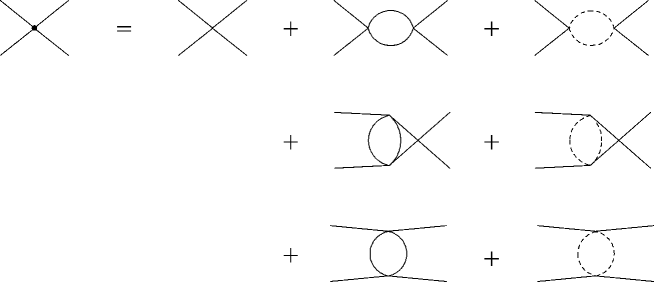
Figure 1: The diagrammatic representation for the effective coupling $\lambda_{\phi}(T)$ up to the one-loop level. The continuous lines stand for the $\phi$ propagators, while the dashed lines represent $\psi$.

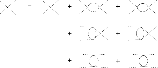
Figure 2: The diagrammatic representation for the effective coupling $\lambda_{\psi}(T)$ up to the one-loop level.

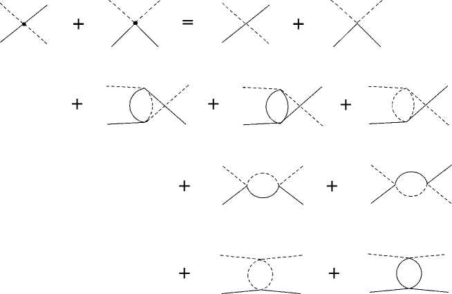
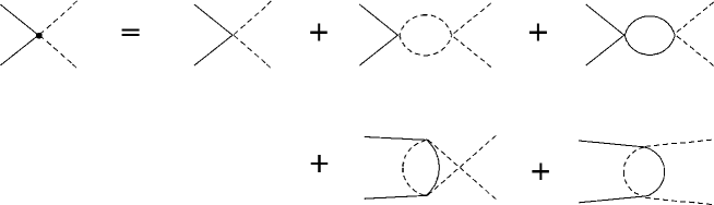
(a) (b) (c)

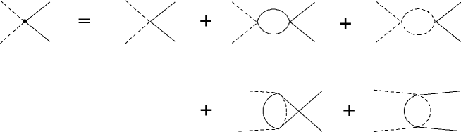
Figure 3: Diagrams contributing up to the one-loop level to the effective cross-coupling $\lambda(T)$. For convenience we have identified the processes: (a) $\phi\psi\to\phi\psi$, (b) $\phi\phi\to\psi\psi$ and (c) $\psi\psi\to\phi\phi$.

Let us now check the robustness of SNR/ISB when the effective, temperature dependent couplings are considered. The thermal effects on all the three couplings, at the one-loop order, are considered in terms of the corrections to the four-point 1PI Green’s functions. All diagrams at the one-loop level contributing to the effective couplings $\lambda_{\phi}(T)$, $\lambda_{\psi}(T)$ and $\lambda(T)$ are shown in Figs. 1, 2 and 3, respectively. These diagrams, with zero external momenta , are easily computed at finite temperature (see for instance Refs. fendley ; roos ). Using again the high temperature approximation at leading order, one obtains

$$\lambda_{\phi}(T)\simeq\lambda_{\phi}+\frac{3}{8\pi^{2}}\ln\left(\frac{T}{M_{0}}\right)\left[\frac{1}{2}\left(\frac{N_{\phi}+8}{9}\right)\lambda_{\phi}^{2}+\frac{N_{\psi}}{2}\lambda^{2}\right]\;,$$ (9)

$$\lambda_{\psi}(T)\simeq\lambda_{\psi}+\frac{3}{8\pi^{2}}\ln\left(\frac{T}{M_{0}}\right)\left[\frac{1}{2}\left(\frac{N_{\psi}+8}{9}\right)\lambda_{\psi}^{2}+\frac{N_{\phi}}{2}\lambda^{2}\right]\;,$$ (10)

and

$$\lambda(T)\simeq\lambda+\frac{\lambda}{8\pi^{2}}\ln\left(\frac{T}{M_{0}}\right)\left[\frac{1}{2}\left(\frac{N_{\phi}+2}{3}\right)\lambda_{\phi}+\frac{1}{2}\left(\frac{N_{\psi}+2}{3}\right)\lambda_{\psi}\right]+\frac{\lambda^{2}}{4\pi^{2}}\ln\left(\frac{T}{M_{0}}\right)\;,$$ (11)

where $M_{0}$ is a regularization scale. In writing the above equations we are once again assuming that the tree-level couplings in Eqs. (9), (10) and (11) are the renormalized ones and we also are only showing the relevant high temperature corrections. The same expressions were also obtained by Roos in roos (note however that different normalizations for the tree-level potential as well as $M_{0}=T_{0},\;N_{\phi}=N_{\psi}=1$ were used in that reference). In roos , the numerical solution of the one-loop Wilson renormalization group equations was also compared to the usual flow equations for the constants obtained from the one-loop beta-functions and shown to agree well with each other up to very high scales. The flow equations referring to the perturbative effective coupling constants Eqs. (9), (10) and (11) are expressed in term of the dimensionless scale $T/M_{0}$ fendley as

$$\frac{d\lambda_{\phi}(t)}{dt}=\frac{3}{8\pi^{2}}\left[\frac{1}{2}\left(\frac{N_{\phi}+8}{9}\right)\lambda_{\phi}^{2}(t)+\frac{N_{\psi}}{2}\lambda^{2}(t)\right]\;,$$ (12)

$$\frac{d\lambda_{\psi}(t)}{dt}=\frac{3}{8\pi^{2}}\left[\frac{1}{2}\left(\frac{N_{\psi}+8}{9}\right)\lambda_{\psi}^{2}(t)+\frac{N_{\phi}}{2}\lambda^{2}(t)\right]\;,$$ (13)

and

$$\frac{d\lambda(t)}{dt}=\frac{\lambda(t)}{8\pi^{2}}\left[\frac{1}{2}\left(\frac{N_{\phi}+2}{3}\right)\lambda_{\phi}(t)+\frac{1}{2}\left(\frac{N_{\psi}+2}{3}\right)\lambda_{\psi}(t)\right]+\frac{\lambda^{2}(t)}{4\pi^{2}}\;,$$ (14)

where $t=\ln(T/M_{0})$ was used. The solutions of the flow equations (12), (13) and (14), with initial conditions given by the renormalized tree-level coupling constants, can also be easily seen to be equivalent to the solutions for the set of linear coupled equations,

$$\lambda_{\phi}(T) = \lambda_{\phi}+\frac{3}{8\pi^{2}}\ln\left(\frac{T}{M_{0}}\right)\left[\frac{1}{2}\left(\frac{N_{\phi}+8}{9}\right)\lambda_{\phi}\lambda_{\phi}(T)+\frac{N_{\psi}}{2}\lambda\lambda(T)\right]\;,$$

$$\lambda_{\psi}(T) = \lambda_{\psi}+\frac{3}{8\pi^{2}}\ln\left(\frac{T}{M_{0}}\right)\left[\frac{1}{2}\left(\frac{N_{\psi}+8}{9}\right)\lambda_{\psi}\lambda_{\psi}(T)+\frac{N_{\phi}}{2}\lambda\lambda(T)\right]\;,$$

$$\lambda(T) = \lambda+\frac{\lambda}{16\pi^{2}}\ln\left(\frac{T}{M_{0}}\right)\left[\frac{1}{2}\left(\frac{N_{\phi}+2}{3}\right)\lambda_{\phi}(T)+\frac{1}{2}\left(\frac{N_{\psi}+2}{3}\right)\lambda_{\psi}(T)\right]$$ (15)

$$+ \frac{\lambda(T)}{16\pi^{2}}\ln\left(\frac{T}{M_{0}}\right)\left[\frac{1}{2}\left(\frac{N_{\phi}+2}{3}\right)\lambda_{\phi}+\frac{1}{2}\left(\frac{N_{\psi}+2}{3}\right)\lambda_{\psi}\right]+\frac{1}{4\pi^{2}}\ln\left(\frac{T}{M_{0}}\right)\lambda\lambda(T)\;.$$

The results obtained from the flow equations given above, or equivalently from the solutions of coupled set of equations (15), are standard ways of nonperturbatively resumming the leading order corrections (in this case the leading log temperature dependent corrections) to the coupling constants. For instance, Eq. (15) is exactly the analogous procedure used for the one-field case for summing all ladder (1-loop or bubble) contributions to the effective coupling constant. For the multi-field case, the perturbative approximation for (15) is again given by Eqs. (9), (10) and (11) at the one-loop level. In our case, these equations are useful to test how robust is the phenomena of SNR/ISB and will be used below in our analysis. Later, in the next section for the nonrelativistic limit of Eq. (1), we will also construct the analogous of these nonperturbative equations for the temperature dependent effective couplings.

In terms of the effective temperature dependent couplings, $\lambda_{\phi}(T)$, $\lambda_{\psi}(T)$ and $\lambda(T)$ the quantity analogous to Eq. (7) becomes

$$\Delta_{i}(T)=\lambda_{i}(T)\frac{1}{2}\left(\frac{N_{i}+2}{3}\right)+\lambda(T)\frac{N_{j}}{2}\;,$$ (16)

or, more explicitly, using Eqs. (9), (10) and (11),

$$\Delta_{i}(T) = \lambda_{i}\left(\frac{N_{i}+2}{6}\right)+\lambda\frac{N_{j}}{2}+\lambda_{i}^{2}\frac{(N_{i}+8)(N_{i}+2)}{288\pi^{2}}\ln\left(\frac{T}{M_{0}}\right)+\lambda N_{j}\frac{(N_{i}+2)\lambda_{i}+(N_{j}+2)\lambda_{j}}{96\pi^{2}}\ln\left(\frac{T}{M_{0}}\right)$$ (17)

$$+ \lambda^{2}\frac{N_{j}(N_{i}+6)}{32\pi^{2}}\ln\left(\frac{T}{M_{0}}\right)\;.$$

It is clear from the expressions for the effective couplings, Eqs. (9), (10), (11) and Eq. (17), that for perturbative values for the tree-level coupling parameters the predicted results for SNR/ISB are very stable even for very large temperatures (in units of the regularization scale $M_{0}$) which is due to the slow logarithmic change with the temperature. As an illustration, consider for example the tree-level coupling parameters that satisfy the boundness condition Eq. (2), $\lambda_{\phi}=7\times 10^{-5}$, $\lambda_{\psi}=5\times 10^{-4}$ and $\lambda=-6\times 10^{-5}$ and $N_{\phi}=N_{\psi}=2$. For these values of parameters Eq. (6) is satisfied and the one-loop equations for the effective masses predict ISB or SNR, along the $\phi$ direction, for $m^{2}_{\phi}>0$ or $m_{\phi}^{2}<0$, respectively. Fig. 4 shows that the boundness condition also holds true for the effective temperature dependent couplings. Fig. 5 shows the quantity $\Delta_{\phi}(T)$, defined by Eq. (16), which remains negative for the whole range of temperatures considered, thus predicting SNR/ISB along the $\phi$ direction, in accordance with the WRG results roos . At the same time, $\Delta_{\psi}(T)$, shown in Fig. 6, remains always positive.

Note that the apparent almost constancy in a wide range of temperatures seem from the Figs. 4, 5 and 6 is only a consequence of the effective couplings be only logarithmically dependent on $T$ and the very small values for the tree-level couplings that we have considered. Had we taken larger values for the tree-level couplings, obviously would lead to a much larger variation with increasing temperature.

Figure 4: The boundness condition, Eq. (2), expressed in terms of the effective couplings, is shown in the vertical axis as the ratio $R(T)=\lambda_{\phi}(T)\lambda_{\psi}(T)/[3\lambda(T)]^{2}$. The temperature is shown in units of the regularization scale $M_{0}$ while $N_{\phi}=N_{\psi}=2$. The tree-level values $\lambda_{\phi}=7\times 10^{-5}$, $\lambda_{\psi}=5\times 10^{-4}$ and $\lambda=-6\times 10^{-5}$ were considered.

Figure 5: The quantity $\Delta_{\phi}(T)$ as a function of the temperature for the same values of parameters considered in Fig. 4.

Figure 6: The quantity $\Delta_{\psi}(T)$ as a function of the temperature for the same values of parameters considered in Fig. 4.

Given the results shown above for the relativistic case, we can conclude, therefore, that the inclusion of thermal effects on the couplings does not exclude the possibility of SNR/ISB occurring at high temperatures. We recall that although the results were obtained with the one-loop approximation this feature does not seem to be an artifact of perturbation theory as confirmed by the results produced by nonperturbative methods, such as the Wilson Renormalization Group procedure used in Ref. roos , as well as the optimized perturbation theory used in Ref. MR1 , where not only thermal corrections to the couplings are accounted for but also to the masses (like in the Schwinger-Dyson or gap equations for the masses).

III SEARCHING FOR SNR/ISB PATTERNS IN THE nonrelativistic CASE

We now turn our attention to the analysis of similar SNR/ISB phenomena displayed by the relativistic model, given by the lagrangian density, Eq. (1), in the case of its nonrelativistic counterpart. Let us first recall some fundamental differences between relativistic and nonrelativistic theories that will be important in our analysis. Firstly, the obvious reduction from Lorentz to Galilean invariance. Secondly, it should be noted that in the nonrelativistic description particle number is conserved and so, only complex fields are allowed. This second point will be particularly important to us since, for the processes entering in the effective couplings shown in Figs. 1, 2 and 3, only those that do not change particle number (the elastic processes) will be allowed (e.g. this selects the processes (a) shown in Fig. 3 but not the (b) and (c), inelastic, ones). Another important difference between relativistic and nonrelativistic models concerns the structure of the respective propagators. While the relativistic propagator allows for both forward and backward particle propagation (which is associated to particles and anti-particles, respectively), the nonrelativistic propagator of scalar theories at $T=0$ only has forward propagation (see e.g. the discussion in Ref. oren ). Note however that the structure of the propagators (or two-point Green’s function) in a thermal bath includes both backward and forward propagation mahan , which can be interpreted in terms of excitations to and from the thermal bath (or, equivalently, emission and absorption of particle to and from the thermal bath KB ).

We should also say that, alternatively to the derivation of the nonrelativistic analog of (1), we could as well consider the relevant equations leading e.g. to the derived effective couplings in the previous section and take the appropriate low-energy limit for those equations. However it is more practical, and indeed it is the procedure usually adopted in atomic and low energy nuclear physics, to start directly from the nonrelativistic Hamiltonian or Lagrangian densities. This is an one step procedure leading, say, to the Feynman rules that can be applied to any other quantity that we may be interested in computing, without having first to compute the corresponding relativistic expressions and then working out the corresponding nonrelativistic. So, let us now initially consider the nonrelativistic limit of the lagrangian density given by Eq. (1). This can be obtained by first expressing the fields $\phi$ and $\psi$ in terms of (complex) nonrelativistic fields $\Phi$ and $\Psi$ as oren ; davis ; zee

$$\phi({\vec{x}},t)=\frac{1}{\sqrt{2m_{\phi}}}\left[\exp(-im_{\phi}t)\Phi({\vec{x}},t)+\exp(im_{\phi}t)\Phi^{*}({\vec{x}},t)\right]\;,$$ (18)

and

$$\psi({\vec{x}},t)=\frac{1}{\sqrt{2m_{\psi}}}\left[\exp(-im_{\psi}t)\Psi({\vec{x}},t)+\exp(im_{\psi}t)\Psi^{*}({\vec{x}},t)\right]\;,$$ (19)

where it is assumed that the fields $\Phi$ and $\Psi$ oscillate in time much more slowly than $\exp(im_{\phi}t)$ and $\exp(im_{\psi}t)$, respectively. By substituting (18) and (19) in (1) and taking the nonrelativistic limit of large masses, the oscillatory terms with frequencies $m_{\phi}$ and $m_{\psi}$ can be dropped. The resulting lagrangian density in terms of $\Phi$, $\Psi$ and complex conjugate fields becomes

$${\cal L}(\Phi^{*},\Phi,\Psi^{*},\Psi) = \frac{1}{2m_{\phi}}\left[-im_{\phi}(\partial_{t}\Phi^{*})\Phi+im_{\phi}\Phi^{*}(\partial_{t}\Phi)-|\nabla\Phi|^{2}+\left|\partial_{t}\Phi\right|^{2}\;\right]-\frac{\lambda_{\phi}}{16m_{\phi}^{2}}(\Phi^{*}\Phi)^{2}$$ (20)

$$+ \frac{1}{2m_{\phi}}\left[-im_{\psi}(\partial_{t}\Psi^{*})\Psi+im_{\psi}\Psi^{*}(\partial_{t}\Psi)-|\nabla\Psi|^{2}+\left|\partial_{t}\Psi\right|^{2}\;\right]-\frac{\lambda_{\psi}}{16m_{\psi}^{2}}(\Psi^{*}\Psi)^{2}$$

$$- \frac{\lambda}{4m_{\phi}m_{\psi}}(\Phi^{*}\Phi)(\Psi^{*}\Psi)\;,$$

where we have assumed for simplicity, in the derivation of the last term in (20), the cross-fields interaction term, that $m_{\phi}\neq m_{\psi}$ . By further considering

$$\left|\partial_{t}\Phi\right|^{2}\ll 2m_{\phi}{\rm Im}(\Phi\partial_{t}\Phi^{*})\;,$$

$$\left|\partial_{t}\Psi\right|^{2}\ll 2m_{\psi}{\rm Im}(\Psi\partial_{t}\Phi^{*})\;,$$ (21)

we can omit the terms with two time derivatives in Eq. (20). So the Lorentz invariance in (20) is lost and the nonrelativistic analogue of (1) is obtained. The interaction terms in Eq. (20) are the same as those obtained by approximating the usual nonrelativistic two-body interaction potentials by hard core (delta) potentials, e.g.,

$$\int d^{3}x\Phi^{*}({\bf x},t)\Phi({\bf x},t)V_{\Phi}({\bf x}-{\bf x}^{\prime})\Phi^{*}({\bf x}^{\prime},t)\Phi({\bf x}^{\prime},t)\to g_{\Phi}\left[\Phi^{*}({\bf x},t)\Phi({\bf x},t)\right]^{2}\;,$$

$$\int d^{3}x\Psi^{*}({\bf x},t)\Psi({\bf x},t)V_{\Psi}({\bf x}-{\bf x}^{\prime})\Psi^{*}({\bf x}^{\prime},t)\Psi({\bf x}^{\prime},t)\to g_{\Psi}\left[\Psi^{*}({\bf x},t)\Psi({\bf x},t)\right]^{2}\;,$$

$$\int d^{3}x\Phi^{*}({\bf x},t)\Phi({\bf x},t)V_{\Phi\Psi}({\bf x}-{\bf x}^{\prime})\Psi^{*}({\bf x}^{\prime},t)\Psi({\bf x}^{\prime},t)\to g_{\Phi\Psi}\left[\Phi^{*}({\bf x},t)\Phi({\bf x},t)\right]\left[\Psi^{*}({\bf x},t)\Psi({\bf x},t)\right]\;.$$ (22)

The approximation of the two-body potential interactions like in (22) is also commonly adopted in the description of cold dilute atomic systems, where only binary type interactions at low energy are relevant. In that case, the local coupling parameters $g_{\Phi},g_{\Psi}$ and $g_{\Phi\Psi}$ are also associated to the s-wave scattering lengths $a_{i}$ bec , e.g., $g_{i}=2\pi a_{i}/m_{i}$. For nonrelativistic systems in general, besides the two-body interaction terms like (22) (in the hard core approximation) we can also include additional one-body like interaction terms, e.g., $\kappa_{\Phi}\Phi^{*}\Phi$, etc. This is the case when we submit the system to an external potential (for example a magnetic field). It can also represent an internal energy term (like the internal molecular energy relative to free atoms in which case the fields in the lagrangian would be related to molecular dimers). In models of superconductivity a constant one-body like interaction term represents the opening of an explicit gap of energy in the system. In the grand-canonical formulation $\kappa_{i}$ can represent chemical potentials included in the action formulation, so that one can also describe density effects (in addition to those from the temperature). In order to retain the symmetry breaking analogies to the previous relativistic model (1), and since our intention here is to keep the analysis as general as possible, we shall also consider additional one-body interaction terms for $\Phi$ and $\Psi$ while their precise interpretation is left as open and will depend on the particular system Eq. (20) is intented to represent.

With the considerations assumed above, we therefore take the following nonrelativistic lagrangian model, that is analogue to the relativistic model Eq. (1),

$${\cal L}(\Phi^{*},\Phi,\Psi^{*},\Psi) = \Phi^{*}\left(i\partial_{t}+\frac{1}{2m_{\Phi}}\nabla^{2}\right)\Phi-\kappa_{\Phi}\Phi^{*}\Phi-\frac{g_{\Phi}}{3!}(\Phi^{*}\Phi)^{2}$$ (23)

$$+ \Psi^{*}\left(i\partial_{t}+\frac{1}{2m_{\Psi}}\nabla^{2}\right)\Psi-\kappa_{\Psi}\Psi^{*}\Psi-\frac{g_{\Psi}}{3!}(\Psi^{*}\Psi)^{2}$$

$$- g(\Phi^{*}\Phi)(\Psi^{*}\Psi)\;,$$

where we have expressed the derivative terms in their more common form (by doing an integration by parts in the action context). The numerical factors and signs in the one and two-body potential terms in (23) have been chosen in such a way so that the potential in (23) are analogous the one considered in (1). The coupling constants shown in (23) are related to those in (20) by $g_{i}=3\lambda_{i}/(8m_{i}^{2})$ (with $i=\Phi,\Psi$) and $g=\lambda/(4m_{\Phi}m_{\Psi})$ while $m_{\Phi}$ and $m_{\Psi}$ represent the (atomic) masses. In addition, notice that for the nonrelativistic limit which leads to Eq. (23) to be valid, one must keep $T\ll m_{i}$. Since for nonrelativistic systems in general, the masses $m_{i}$ are of order of typical atomic masses, $m_{i}\sim{\cal O}(1-100){\rm GeV}$, and the typical temperatures in condensed matter systems are at most of order of a few eV, this condition will always hold for the ranges of temperature we will be interested in below.

For multi-component fields, Eq. (23) is the nonrelativistic multi-scalar model with symmetry $U(N_{\Phi})\times U(N_{\Psi})$ that is the analogue of the original relativistic model Eq. (1). For simplicity, in the following we assume the simplest version of (23) where $N_{\Phi}=N_{\Psi}=1$, corresponding to an $U(1)\times U(1)$ symmetric model. In this case, by writing the complex fields in terms of real components,

$$\Phi=\frac{1}{\sqrt{2}}\left(\phi_{1}+i\phi_{2}\right)\;,\;\;\;\Psi=\frac{1}{\sqrt{2}}\left(\psi_{1}+i\psi_{2}\right)\;,$$ (24)

we see that the lagrangian model (23) falls in the same class of universality as that of Eq. (1) for the case of the $O(2)\times O(2)$ symmetry. The extension to higher symmetries can be done starting from (23) but the case of simplest symmetry involving the coupling of complex scalar fields will already be sufficient for our study (physically, this system may, for example, describe the coupling of Bose atoms or molecules in an atomic dilute gas system).

Just like in the relativistic case, in the current application we consider the $\kappa_{i}$, that appears in Eq. (23), as simple temperature independent parameters for which thermal corrections arise from the evaluation of the corresponding field self-energies. Now, to make contact with the analogous potential used in the prototype relativistic models for SNR/ISB, we take the overall potential as being repulsive, bounded from below. This requirement imposes a constraint condition analogous to the one found in the relativistic case, $g_{\Psi}>0$, $g_{\Phi}>0$ and $g_{\Psi}g_{\Phi}>9g^{2}$. At a given temperature, the phase structure of the model is then given by the sign of $\kappa_{i}(T)=\kappa_{i}+\Sigma_{i}$, where $\Sigma_{i}$ is the field temperature dependent self-energy. In the broken phase $\kappa_{i}(T)<0$, while in the symmetric phase $\kappa_{i}(T)>0$. The phase transition occurs at $\kappa_{i}(T=T_{c}^{i})=0$. At the one-loop level the diagrams contributing to the field self-energies are the same as those in the relativistic case. The main difference is that the momentum integrals in the loops are now given in terms of the nonrelativistic propagators for $\Phi$ and $\Psi$,

$$D_{i}(\omega_{n},{\bf q})=\frac{1}{-i\omega_{n}+\omega_{i}({\bf q})}\;,$$ (25)

where $\omega_{n}=2\pi nT$ ($n=0,\pm 1,\pm 2,\ldots$) are the bosonic Matsubara frequencies and $\omega_{i}({\bf q})={\bf q}^{2}/(2m_{i})+\kappa_{i}$. At the one-loop level we then obtain (see appendix)

$$\Sigma_{i}(T)=T\sum_{n=-\infty}^{+\infty}\int\frac{d^{3}q}{(2\pi)^{3}}\left[\frac{2g_{i}/3}{-i\omega_{n}+\omega_{i}({\bf q})}+\frac{g}{-i\omega_{n}+\omega_{j}({\bf q})}\right],$$ (26)

The sum in Eq. (26) can be easily performed and the resulting momentum integrals lead to well known Bose integrals (see e.g. Ref. pathria and also the appendix for the derivations of these equations). We then obtain the results

$$\kappa_{\Phi}(T)=\kappa_{\Phi}+\frac{2g_{\Phi}}{3}\left(\frac{m_{\Phi}T}{2\pi}\right)^{3/2}{\rm Li}_{3/2}[\exp(-\kappa_{\Phi}/T)]+g\left(\frac{m_{\Psi}T}{2\pi}\right)^{3/2}{\rm Li}_{3/2}[\exp(-\kappa_{\Psi}/T)]\;,$$ (27)

and

$$\kappa_{\Psi}(T)=\kappa_{\Psi}+\frac{2g_{\Psi}}{3}\left(\frac{m_{\Psi}T}{2\pi}\right)^{3/2}{\rm Li}_{3/2}[\exp(-\kappa_{\Psi}/T)]+g\left(\frac{m_{\Phi}T}{2\pi}\right)^{3/2}{\rm Li}_{3/2}[\exp(-\kappa_{\Phi}/T)]\;,$$ (28)

where ${\rm Li}_{n}(z_{i})$ is the polylogarithmic function. Like in the relativistic effective mass terms, in Eqs. (27) and (28) we have once again limited to showing the temperature dependent corrections coming from $\Sigma_{i}$, omitting the divergent (zero-point energy terms) contributions to the effective one-body terms (so the tree-level parameters in Eqs. (27) and (28) are assumed to be already the renormalized ones). Let us now consider the high temperature approximation, which in the nonrelativistic case is valid as long as $\kappa_{i}\ll T\ll m_{i}$. Then, one is allowed to consider the approximation for the polylogarithmic functions in Eqs. (27) and (28), ${\rm Li}_{3/2}[\exp(-\kappa_{i}/T)]\sim\zeta(3/2)$, where $\zeta(x)$ is the Riemann zeta function and $\zeta(3/2)\simeq 2.6124$. One can then write the two equations (27) and (28) in the high temperature approximation more compactly, as

$$\kappa_{i}(T)\simeq\kappa_{i}+\left(\frac{T}{2\pi}\right)^{3/2}\zeta(3/2)\Delta^{\rm NR}_{i}\;,$$ (29)

where we defined the quantity $\Delta^{\rm NR}_{i}$ analogous to that of the relativistic case,

$$\Delta^{\rm NR}_{i}=\frac{2}{3}g_{i}m_{i}^{3/2}+gm_{j}^{3/2}\;,$$ (30)

in terms of which we obtain the critical temperature for symmetry restoration/breaking analogous to the relativistic expression,

$$T_{c,i}^{\rm NR}=2\pi\left[\frac{-\kappa_{i}}{\Delta^{\rm NR}_{i}\zeta(3/2)}\right]^{2/3}\;.$$ (31)

Eq. (31) shows that there are three interesting cases which depend on the sign and magnitude of the cross coupling $g$. Taking $\kappa_{i}<0$ and $g>0$ one observes a shift in the critical temperatures indicating that the transition occurs at lower temperatures compared to the decoupled case ($g=0$). If $g<0$ but $|g|<(2/3)g_{i}(m_{i}/m_{j})^{3/2}$ then the transition occurs at higher temperatures. Despite these quantitative differences symmetry restoration does take place in both cases. Now consider for instance the case, with $\kappa_{\Phi}<0$, where $g<0$ but $|g|>(2/3)g_{\Phi}(m_{\Phi}/m_{\Psi})^{3/2}$ (in this case, and assuming $m_{\Phi}\sim m_{\Psi}$, the boundness condition assures that $|g|<(2/3)g_{\Psi}$). Under these conditions, for the $\Phi$ field we have a similar situation as that for the corresponding relativistic case studied in Sec. II, where, Eq. (31) does not give a finite, positive real quantity. This is a manifestation of ISB (for $\kappa_{\Phi}<0$, or SNR, for $\kappa_{\Phi}>0$) within our two-field complex nonrelativistic model being analogous to what is seen in the relativistic case. At the same time the field $\Psi$ suffers the expected phase transition at a higher $T_{c}$ compared to the $g=0$ case. As in the relativistic case, which field will suffer SNR/ISB depends on our initial choice of parameters in the tree level potential, so it is model dependent. The SNR/ISB result as seen above in this nonrelativistic model is however misleading, as we next show by considering the same phenomenon in terms of the effective, temperature dependent, coupling parameters.

Physically, the possibility of SNR/ISB occurring at high temperatures as predicted by the naive perturbative approximation, Eq. (29), is much harder to be accepted in the nonrelativistic case (condensed matter) than in the relativistic case (cosmology), which already seems to indicate that the results here should be different when the simple perturbative calculations are improved.

Following the analogy with the relativistic model calculation done in Sec. II, we next evaluate the temperature effects on the nonrelativistic couplings.

The diagrams contributing to the effective self-couplings $g_{\Phi}(T)$ and $g_{\Psi}(T)$, at the one-loop level, are those shown in Figs. 1 and 2, respectively, except that the s-channel ones with internal propagators for fields different from those in the external legs (the second one-loop diagrams in Figs. 1 and 2 made of vertices nonconserving particles) are absent. For the effective cross-coupling $g(T)$, as discussed at the beginning of this section, the diagrams contributing at the one-loop level are the ones shown in Fig. 3(a), corresponding to the particle number preserving processes. Using (25) for the nonrelativistic field propagators, the explicit expressions for the effective couplings at one-loop order are found to be (see also the appendix)

$$g_{\Phi}(T)=g_{\Phi} - \frac{g_{\Phi}^{2}}{3}\int\frac{d^{3}{\bf q}}{(2\pi)^{3}}\frac{1}{2\omega_{\Phi}({\bf q})}\left\{1+2n(\omega_{\Phi})+8\beta\omega_{\Phi}n(\omega_{\Phi})\left[1+n(\omega_{\Phi})\right]\right\}$$ (32)

$$- 3g^{2}\int\frac{d^{3}{\bf q}}{(2\pi)^{3}}\beta n(\omega_{\Psi})\left[1+n(\omega_{\Psi})\right]\;,$$

$$g_{\Psi}(T)=g_{\Psi} - \frac{g_{\Psi}^{2}}{3}\int\frac{d^{3}{\bf q}}{(2\pi)^{3}}\frac{1}{2\omega_{\Psi}({\bf q})}\left\{1+2n(\omega_{\Psi})+8\beta\omega_{\Psi}n(\omega_{\Psi})\left[1+n(\omega_{\Psi})\right]\right\}$$ (33)

$$- 3g^{2}\int\frac{d^{3}{\bf q}}{(2\pi)^{3}}\beta n(\omega_{\Phi})\left[1+n(\omega_{\Phi})\right]\;,$$

and

$$g(T)=g - \frac{2g}{3}\int\frac{d^{3}{\bf q}}{(2\pi)^{3}}\beta\left\{g_{\Phi}n(\omega_{\Phi})\left[1+n(\omega_{\Phi})\right]+g_{\Psi}n(\omega_{\Psi})\left[1+n(\omega_{\Psi})\right]\right\}$$ (34)

$$- g^{2}\int\frac{d^{3}{\bf q}}{(2\pi)^{3}}\left\{\frac{\omega_{\Psi}}{\omega_{\Psi}^{2}-\omega_{\Phi}^{2}}\left[1+2n(\omega_{\Phi})\right]-\frac{\omega_{\Phi}}{\omega_{\Psi}^{2}-\omega_{\Phi}^{2}}\left[1+2n(\omega_{\Psi})\right]\right\}\;.$$

The numerical factors in Eqs. (32), (33) and (34) are due to the symmetries of the diagrams and normalizations chosen in Eq. (23). $n(\omega)$ in the above equations is the Bose-Einstein distribution.

The zero temperature contributions in Eqs. (32) - (34) are divergent and require proper renormalization. This is mostly simply done by performing the momentum integrals in $d=3-\epsilon$ dimensions and the resulting integrals are all found to be finite in dimensional regularization (when taking $\epsilon\to 0$ at the end). The momentum integrals for the finite temperature contributions in Eqs. (32) - (34) can again be performed with the help of the Bose integrals given in the appendix. We can further simplify the equations by considering parameters such as $m_{\Phi}\simeq m_{\Psi}=m$, $\kappa_{\Phi}\simeq\kappa_{\Psi}=\kappa$ and temperatures satisfying $\kappa\ll T\ll m$ in which case the zero temperature corrections to the couplings are negligible compared to the finite temperature ones and can safely be neglected. At leading order, in $T$, we then obtain the results

$$g_{\Phi}(T)\simeq g_{\Phi}-\frac{mT}{12\pi}\sqrt{\frac{2m}{\kappa}}\left(5g_{\Phi}^{2}+9g^{2}\right)+{\cal O}(\kappa/T)\;,$$ (35)

$$g_{\Psi}(T)\simeq g_{\Psi}-\frac{mT}{12\pi}\sqrt{\frac{2m}{\kappa}}\left(5g_{\Psi}^{2}+9g^{2}\right)+{\cal O}(\kappa/T)\;,$$ (36)

and

$$g(T)\simeq g-\frac{mT}{4\pi}\sqrt{\frac{2m}{\kappa}}g\left(g+\frac{2g_{\Phi}}{3}+\frac{2g_{\Psi}}{3}\right)+{\cal O}(\kappa/T)\;.$$ (37)

Note from Eqs. (35), (36) and (37) that the effective couplings in the nonrelativistic theory have a much stronger dependence with the temperature than in those in the equivalent relativistic theory, Eqs. (9), (10) and (11). We therefore expect to see larger deviations at high temperatures for the effective couplings as compared with the same case in the relativistic problem (by high temperature we mean here temperatures larger than the typical one-body potential coefficients in (23), but much less than the particle masses, see above). It is also evident from the analysis of higher loop corrections to the effective couplings in the nonrelativistic model that all bubble like corrections contribute with the same power in temperature as the one-loop terms, which can easily be checked by simple power-counting in the momentum. A side effect of this is the breakdown, at high temperatures, of the simple one-loop perturbation theory applied here. Another symptom is the apparent running of the effective self-couplings, shown above, to negative values for sufficiently high temperatures given by $T\gtrsim T_{\rm break}\sim{\rm min}\left(12\pi\sqrt{\kappa/(2m^{3})}g_{\Phi}/(5g_{\Phi}^{2}+9g^{2}),\;12\pi\sqrt{\kappa/(2m^{3})}g_{\Psi}/(5g_{\Psi}^{2}+9g^{2})\right)$. Nevertheless, it is easy to check that (for the parameters adopted below) the results obtained by just plugging Eqs. (35), (36) and (37) above into Eqs. (29) already show a drastic qualitative difference between this simple improved approximation and the naive perturbative evaluation given by Eq. (29). It looks that for the nonrelativistic case SNR/ISB is a mere artifact of perturbation theory. Intuitively, this is already a rather satisfactory result which, as we will show below, will be confirmed by a nonperturbative resummation of the bubble like corrections. The resumming of all leading order bubble corrections to the couplings can again be done by solving the set of homogeneous linear equations for $g_{\Phi}(T),g_{\Psi}(T)$ and $g(T)$,

$$g_{\Phi}(T) = g_{\Phi}-g_{\Phi}(T)\,\frac{g_{\Phi}}{3}\;I_{1}(\beta\kappa_{\Phi})-3g(T)\,g\;I_{2}(\beta\kappa_{\Psi})\,\,,$$

$$g_{\Psi}(T) = g_{\Psi}-g_{\Psi}(T)\,\frac{g_{\Psi}}{3}\;I_{1}(\beta\kappa_{\Psi})-3g(T)\,g\;I_{2}(\beta\kappa_{\Phi})\,\,,$$

$$g(T) = g-g(T)\,\frac{2g_{\Phi}}{6}\;I_{2}(\beta\kappa_{\Phi})-g(T)\,\frac{2g_{\Psi}}{6}\;I_{2}(\beta\kappa_{\Psi})-g_{\Phi}(T)\,\frac{2g}{6}\;I_{2}(\beta\kappa_{\Phi})-g_{\Psi}(T)\,\frac{2g}{6}\;I_{2}(\beta\kappa_{\Psi})\,\,,$$ (38)

$$- g(T)\;g\;I_{3}(\beta\kappa_{\Phi},\beta\kappa_{\Psi})\;,$$

where we have defined the functions

$$I_{1}(\beta\kappa_{i}) = \int\frac{d^{3}{\bf q}}{(2\pi)^{3}}\frac{1}{2\omega_{i}({\bf q})}\left\{1+2n(\omega_{i})+8\beta\omega_{i}n(\omega_{i})\left[1+n(\omega_{i})\right]\right\}\;,$$

$$I_{2}(\beta\kappa_{i}) = \int\frac{d^{3}{\bf q}}{(2\pi)^{3}}\beta n(\omega_{i})\left[1+n(\omega_{i})\right]\;,$$

$$I_{3}(\beta\kappa_{i},\beta\kappa_{j}) = \int\frac{d^{3}{\bf q}}{(2\pi)^{3}}\left\{\frac{\omega_{j}}{\omega_{j}^{2}-\omega_{i}^{2}}\left[1+2n(\omega_{i})\right]-\frac{\omega_{i}}{\omega_{j}^{2}-\omega_{i}^{2}}\left[1+2n(\omega_{j})\right]\right\}\;.$$ (39)

One is now in position to investigate how thermal effects on the effective nonrelativistic couplings manifest themselves in phenomena similar to SNR/ISB. First we show in Fig. 7 some representative results for the effective interactions obtained from the solutions of Eq. (38). The tree-level parameters considered here are: $g_{\Phi}=2\times 10^{-15}{\rm eV}^{-2},g_{\Psi}=10^{-16}{\rm eV}^{-2},g=-10^{-16}{\rm eV}^{-2}$, $m_{\Phi}\simeq m_{\Psi}=1{\rm GeV}$ and $\kappa_{\Phi}=\kappa_{\Psi}=1{\rm neV}$. We note that all couplings tend to evolve to zero at very high temperatures as $T$ gets closer to $m$. So, the apparent instability caused by the fact that $g_{\Psi}(T)$ as well as $g_{\Phi}(T)$ could become negative beyond some temperature, $T_{\rm break}$, as suggested by Eqs. (35) and (36), has disappeared completely when the nonperturbative flow of the couplings are considered (using the tree-level parameters given above and from Eqs. (35) and (36), one would get $T_{\rm break}\sim 0.019$ eV (or $\sim 220$ K)).

It is tempting, by looking at Fig. 7, to associate this to a free model at high energies, however we must recall that the nonrelativistic model, Eq. (23), will eventually no longer be valid for such high values of temperature, in which case it should be replaced by the original relativistic model (in any case the model Eq. (23) should of course be regarded as an effective model valid at low energy scales only).

Figure 7: The non relativistic effective couplings as a function of temperature (shown in units of eV).

In Fig. 8 we show the equivalent of Eq. (30) for the $\Phi$ and $\Psi$ fields, $\Delta_{\Phi}^{\rm NR}(T)$ and $\Delta_{\Psi}^{\rm NR}(T)$, respectively, given in terms of the temperature dependent bubble resummed couplings for the same tree-level parameters considered above. We note that for the parameters considered $\Delta_{\Psi}^{\rm NR}(T)$ is initially negative and reverse sign at some temperature, indicating that symmetry breaking at high temperatures tend to happen in the $\Psi$ field direction, while the potential in the $\Phi$ direction remains unbroken (actually, the temperature where $\Delta_{\Psi}^{\rm NR}(T)$ crosses zero, is close to the point of a reentrant transition for $\Psi$). $\Delta_{\Phi}^{\rm NR}(T)$ however always remain positive, which then points to no transition in the $\Phi$ direction. These aspects are also clearly seen in the plot, shown in Fig. 9, for the effective one-body term $\kappa_{\Psi}(T)$, expressed in terms of the effective nonperturbative couplings. In terms of the parameters considered, symmetry breaking is seen to happen at a temperature $T_{c,\Psi}^{(SB)}\simeq 3.4\times 10^{-4}{\rm eV}$ (or $\sim 4$ K) while the reentrant phase (symmetry restoration) happens at a temperature $T_{c,\Psi}^{(SR)}\simeq 1.4\times 10^{-2}{\rm eV}$ (or $\sim 161$ K). In between these two temperatures we see a manifestation of an ISB phase. In the $\Phi$ direction there is no symmetry breaking or reentrant phases at any temperature for the parameters considered.

Figure 8: The quantities $\Delta_{\Phi}^{\rm NR}(T)/m^{3/2}$ and $\Delta_{\Psi}^{\rm NR}(T)/m^{3/2}$ as a function of the temperature for the same values of parameters used in Fig. 7.

Figure 9: The nonperturbative effective one-body term $\kappa_{\Psi}(T)$ as a function of the temperature for the same values of parameters used in Fig. 7. Both quantities are expressed in units of eV. The arrows indicate the points of SB and SR, with an intermediary ISB phase happening between the temperatures $T_{c}^{\rm SB}<T<T_{c}^{\rm SR}$.

In Fig. 10 we show a phase diagram for the system as a function of the tree-level coupling $g_{\Psi}$ and the temperature. The thin horizontal line at $g_{\Psi}=10^{-16}{\rm eV}^{-2}$ illustrates the reentrant transition (through an inverse symmetry breaking) shown in Fig. 9. All other parameters are the same as considered above. Note that the condition of stability, $g_{\Psi}g_{\Phi}>9g^{2}$, expressed in terms of the nonperturbative and temperature dependent couplings, is always satisfied at any temperature for the parameters considered for the previous figures (the effective couplings $g_{\Psi}$ and $g_{\Phi}$ also remain always positive, as is clear from Fig. 7 and previous discussion).

Figure 10: A phase diagram of the system for fixed parameters: $g_{\Phi}=2\times 10^{-15}{\rm eV}^{-2},g=-10^{-16}{\rm eV}^{-2}$, $m_{\Phi}\simeq m_{\Psi}=1\,{\rm GeV}$ and $\kappa_{\Phi}=\kappa_{\Psi}=1\,{\rm neV}$. The dotted line separates the region of stability ($R^{\rm NR}(T)>1$) from that of instability ($R^{\rm NR}(T)<1$), according to the value of the ratio $R^{\rm NR}(T)=g_{\Psi}(T)g_{\Phi}(T)/[9g^{2}(T)]$. The regions of SR and SB, in the $\Psi$ direction, are also shown. The thin horizontal line indicates the value of $g_{\Psi}$ used in the text.

IV CONCLUSIONS

We have reviewed how symmetry non-restoration and inverse symmetry breaking may take place, at arbitrarily large temperatures, in multi-field scalar relativistic and nonrelativistic theories. These counter intuitive phenomena appear due to the fact that the crossed interaction can be negative while the models are still bounded from below. We have recalled that, in the relativistic case, SNR/ISB are not a mere artifact of calculational approximations. We have then set to investigate the possible SNR/ISB manifestation and consequences in a nonrelativistic $U(N_{\Phi})\times U(N_{\Psi})$ scalar model of hard core spheres by considering the simplest case, $N_{\Phi}=N_{\Psi}=1$, which may be relevant for condensed matter systems of bosonic atoms or molecules.

Performing a naive perturbative one-loop calculation, which includes only the first thermal contribution to the self-energy, we have shown that, for negative values of the crossed coupling, SNR/ISB can take place like in the relativistic case. However, the manifestation of SNR/ISB in condensed matter systems of hard core spheres seems to be more counter intuitive than in the relativistic case where the model may represent, e.g., the Higgs sector. With this in mind we have investigated the explicit (temperature) running of the nonrelativistic couplings. One first improvement was to evaluate the perturbative one-loop thermal corrections to the couplings which already indicate that SNR/ISB do not seem to happen, at high temperatures, for the nonrelativistic case. Next, we have resummed the bubble like contributions in a nonperturbative fashion. This procedure fixed the instability problem related to the possibility of $g_{i}(T)$ becoming negative as observed in the calculation which considered only the simplest one-loop corrections to the couplings. Our nonperturbative calculation also showed that the phase transitions happening in the nonrelativistic case includes a continuous SB/SR pattern characterized, at intermediate temperatures, by a reentrant, continuous transition. Therefore, we can state as our major result that, contrary to the relativistic case, SNR/ISB does not seem to occur in the nonrelativistic model of hard core spheres. Instead, reentrant like phenomena become possible, as our results have indicated.

Finally, it would be interesting to investigate SNR/ISB in connection with the Bose-Einstein condensation problem and the present work gives some of the ideas and tools needed for this task that we hope to pursue and report in a future publication.

Appendix A Temperature dependent corrections for the nonrelativistic model

Here we give the main steps used in the evaluation of the thermal masses and couplings for the nonrelativistic model. Similar derivations for the relativistic model can be found e.g. in Refs. roos ; fendley ; MR1 .

The effective one-body terms $\kappa_{i}(T)$ and the effective couplings (two-body terms) for the nonrelativistic model are most easily to obtain directly from a computation of the one-loop effective potential for the model lagrangian (23). The effective one and two-body terms will then be identified with the appropriate derivatives of the effective potential.

As usual in the computation of the one-loop potential, we start by decomposing the fields $\Phi$ and $\Psi$ in (23) in terms of (constant) background fields (which, without loss of generality, can be taken as real fields) $\phi_{0}$ and $\psi_{0}$, respectively, and fluctuations $\phi$ and $\psi$, which in terms of real components, become

$$\Phi=\frac{1}{\sqrt{2}}\left(\phi_{0}+\phi_{1}+i\phi_{2}\right)\;,$$ (40)

$$\Psi=\frac{1}{\sqrt{2}}\left(\psi_{0}+\psi_{1}+i\psi_{2}\right)\;.$$ (41)

When substituting Eqs. (40) and (41) in (23) we only need keep the quadratic terms in the fluctuation fields for the computation of the one-loop potential for the background fields $\phi_{0}$ and $\psi_{0}$. We then obtain the (Euclidean) lagrangian density in terms of $\phi_{0}$ and $\psi_{0}$,

$${\cal L}_{E} = \frac{\kappa_{\Phi}}{2}\phi_{0}^{2}+\frac{g_{\Phi}}{4!}\phi_{0}^{4}+\frac{\kappa_{\Psi}}{2}\psi_{0}^{2}+\frac{g_{\Psi}}{4!}\psi_{0}^{4}+\frac{g}{4}\phi_{0}^{2}\psi_{0}^{2}$$ (42)

$$+ \frac{1}{2}\chi\cdot\hat{M}\cdot\chi+{\rm cubic\;and\;quartic\;interaction\;terms}\;,$$

where we have defined the vector $\chi=(\phi_{1},\phi_{2},\psi_{1},\psi_{2})$ and $\hat{M}$ is the matrix operator for the quadratic terms in the fluctuations,

$$\hat{M}=\left(\begin{array}[]{cccc}\frac{-\nabla^{2}}{2m_{\Phi}}+\kappa_{\Phi}+\frac{g_{\Phi}}{2}\phi_{0}^{2}+\frac{g}{2}\psi_{0}^{2}&i\partial_{\tau}&g\phi_{0}\psi_{0}&0\\ -i\partial_{\tau}&\frac{-\nabla^{2}}{2m_{\Phi}}+\kappa_{\Phi}+\frac{g_{\Phi}}{6}\phi_{0}^{2}+\frac{g}{2}\psi_{0}^{2}&0&0\\ g\phi_{0}\psi_{0}&0&\frac{-\nabla^{2}}{2m_{\Psi}}+\kappa_{\Psi}+\frac{g_{\Psi}}{2}\psi_{0}^{2}+\frac{g}{2}\phi_{0}^{2}&i\partial_{\tau}\\ 0&0&-i\partial_{\tau}&\frac{-\nabla^{2}}{2m_{\Psi}}+\kappa_{\Psi}+\frac{g_{\Psi}}{6}\psi_{0}^{2}+\frac{g}{2}\phi_{0}^{2}\end{array}\right).$$ (43)

The partial time derivative in (43) is over Euclidean time: $\partial_{\tau}=\partial/\partial\tau$, $\tau=it$. By performing the functional integration in the quadratic fluctuations $\chi$, the one-loop effective potential $V_{\rm eff}(\phi_{0},\psi_{0})$ obtained from Eq. (42) is given by

$$V_{\rm eff}(\phi_{0},\psi_{0})=\frac{\kappa_{\Phi}}{2}\phi_{0}^{2}+\frac{g_{\Phi}}{4!}\phi_{0}^{4}+\frac{\kappa_{\Psi}}{2}\psi_{0}^{2}+\frac{g_{\Psi}}{4!}\psi_{0}^{4}+\frac{g}{4}\phi_{0}^{2}\psi_{0}^{2}+\frac{1}{2}\ln\det\hat{M}\;,$$ (44)

where the last term on the rhs of (44) comes from the functional integral over the components of $\chi$,

$$\frac{1}{2}\ln\det\hat{M}=-\frac{1}{\beta V}\int D\phi_{1}D\phi_{2}D\psi_{1}D\psi_{2}\exp\left[-\int_{0}^{\beta}d\tau\int d^{3}x\left(\frac{1}{2}\chi\cdot\hat{M}\cdot\chi\right)\right]\;,$$ (45)

and $V$ is the volume of space. Expressing Eqs. (45) and (43) in the space-time momentum Fourier transform form, we then also obtain

$$\frac{1}{2}\ln\det\hat{M} = \frac{1}{2}\frac{1}{\beta}\sum_{n}\int\frac{d^{3}{\bf q}}{(2\pi)^{3}}\ln\left\{\left[\omega_{n}^{2}+E_{\Phi}^{2}({\bf q})\right]\left[\omega_{n}^{2}+E_{\Psi}^{2}({\bf q})\right]\right.$$ (46)

$$- \left.g^{2}\phi_{0}^{2}\psi_{0}^{2}\left[\omega_{\Phi}({\bf q})+\frac{g_{\Phi}}{6}\phi_{0}^{2}+\frac{g}{2}\psi_{0}^{2}\right]\left[\omega_{\Psi}({\bf q})+\frac{g_{\Psi}}{6}\psi_{0}^{2}+\frac{g}{2}\phi_{0}^{2}\right]\right\}\;,$$

with

$$E_{\Phi}({\bf q})=\sqrt{\left[\omega_{\Phi}({\bf q})+\frac{g_{\Phi}}{2}\phi_{0}^{2}+\frac{g}{2}\psi_{0}^{2}\right]\left[\omega_{\Phi}({\bf q})+\frac{g_{\Phi}}{6}\phi_{0}^{2}+\frac{g}{2}\psi_{0}^{2}\right]}\;,$$ (47)

and

$$E_{\Psi}({\bf q})=\sqrt{\left[\omega_{\Psi}({\bf q})+\frac{g_{\Psi}}{2}\psi_{0}^{2}+\frac{g}{2}\phi_{0}^{2}\right]\left[\omega_{\Psi}({\bf q})+\frac{g_{\Psi}}{6}\psi_{0}^{2}+\frac{g}{2}\phi_{0}^{2}\right]}\;.$$ (48)

From $V_{\rm eff}(\phi_{0},\psi_{0})$, Eq. (44), we now define the effective one-body terms as

$$\kappa_{\Phi}(T)=\frac{\partial^{2}V_{\rm eff}(\phi_{0},\psi_{0})}{\partial\phi_{0}^{2}}\Bigr{|}_{\phi_{0}=0,\psi_{0}=0}\;,$$ (49)

$$\kappa_{\Psi}(T)=\frac{\partial^{2}V_{\rm eff}(\phi_{0},\psi_{0})}{\partial\psi_{0}^{2}}\Bigr{|}_{\phi_{0}=0,\psi_{0}=0}\;,$$ (50)

which then gives

$$\kappa_{\Phi}(T)=\kappa_{\Phi}+\frac{2g_{\Phi}}{3}\frac{1}{\beta}\sum_{n}\int\frac{d^{3}{\bf q}}{(2\pi)^{3}}\frac{\omega_{\Phi}({\bf q})}{\omega_{n}^{2}+\omega^{2}_{\Phi}({\bf q})}+g\frac{1}{\beta}\sum_{n}\int\frac{d^{3}{\bf q}}{(2\pi)^{3}}\frac{\omega_{\Psi}({\bf q})}{\omega_{n}^{2}+\omega^{2}_{\Psi}({\bf q})}\;,$$ (51)

and

$$\kappa_{\Psi}(T)=\kappa_{\Psi}+\frac{2g_{\Psi}}{3}\frac{1}{\beta}\sum_{n}\int\frac{d^{3}{\bf q}}{(2\pi)^{3}}\frac{\omega_{\Psi}({\bf q})}{\omega_{n}^{2}+\omega^{2}_{\Psi}({\bf q})}+g\frac{1}{\beta}\sum_{n}\int\frac{d^{3}{\bf q}}{(2\pi)^{3}}\frac{\omega_{\Phi}({\bf q})}{\omega_{n}^{2}+\omega^{2}_{\Phi}({\bf q})}\;,$$ (52)

The Eqs. (51) and (52) can also easily be expressed in terms of the free nonrelativistic propagators $D_{\Phi}(\omega_{n},{\bf q})$ and $D_{\Psi}(\omega_{n},{\bf q})$. The sum over the Matsubara frequencies in (51) and (52) are easily performed by using the identity jackiw ,

$$\frac{1}{\beta}\sum_{n}\frac{1}{\omega_{n}^{2}+\omega^{2}}=\frac{1}{\omega}\left[\frac{1}{2}+n(\omega)\right]\;,$$ (53)

where $n(\omega)$ is the Bose-Einstein distribution,

$$n(\omega)=\frac{1}{e^{\beta\omega}-1}\;.$$ (54)

The momentum integrals in Eqs. (51) and (52) can be expressed in terms of standard Bose integrals as follows (see for example pathria ). Consider the integral (where $\omega={\bf q}^{2}/(2m)+\kappa$ and $\eta=\beta\kappa$)

$$\int\frac{d^{3}q}{(2\pi)^{3}}n(\omega) = \frac{1}{2\pi^{2}}\left(\frac{2m}{\beta}\right)^{3/2}\int_{0}^{\infty}dx\,\frac{x^{2}}{e^{x^{2}+\eta}-1}$$ (55)

$$= \frac{1}{2\pi^{2}}\left(\frac{2m}{\beta}\right)^{3/2}\sum_{l=1}^{\infty}e^{-l\eta}\int_{0}^{\infty}dx\,x^{2}e^{-lx^{2}}$$

$$= \left(\frac{m}{2\pi\beta}\right)^{3/2}{\rm Li}_{3/2}\left(e^{-\beta\kappa}\right)\;,$$

where we used the definition for the polylogarithmic function,

$${\rm Li}_{\alpha}(z)=\sum_{l=1}^{\infty}\frac{z^{l}}{l^{\alpha}}\;.$$ (56)

Another useful momentum integral that also can be obtained from (55) is

$$\int\frac{d^{3}q}{(2\pi)^{3}}n(\omega)[1+n(\omega)]=\left(\frac{m}{2\pi\beta}\right)^{3/2}{\rm Li}_{1/2}\left(e^{-\beta\kappa}\right)\;.$$ (57)

We also have the results obtained from the the polylogarithmic functions in the high temperature approximation, $\kappa\ll T$, and that are used in the text,

$${\rm Li}_{3/2}\left(e^{-\beta\kappa}\right)=\zeta(3/2)-2\sqrt{\pi\frac{\kappa}{T}}+{\cal O}(\kappa/T)\;,$$ (58)

and

$${\rm Li}_{1/2}\left(e^{-\beta\kappa}\right)=\sqrt{\pi\frac{T}{\kappa}}-\zeta(1/2)+{\cal O}(\kappa/T)\;.$$ (59)

Using (55) in Eqs. (51) and (52) we obtain the results quoted in the text, Eqs. (27) and (28).

The two-body effective terms are also defined analogously as

$$g_{\Phi}(T)=\frac{\partial^{4}V_{\rm eff}(\phi_{0},\psi_{0})}{\partial\phi_{0}^{4}}\Bigr{|}_{\phi_{0}=0,\psi_{0}=0}\;,$$ (60)

$$g_{\Psi}(T)=\frac{\partial^{4}V_{\rm eff}(\phi_{0},\psi_{0})}{\partial\psi_{0}^{4}}\Bigr{|}_{\phi_{0}=0,\psi_{0}=0}\;,$$ (61)

and

$$g(T)=\frac{\partial^{4}V_{\rm eff}(\phi_{0},\psi_{0})}{\partial\phi_{0}^{2}\partial\psi_{0}^{2}}\Bigr{|}_{\phi_{0}=0,\psi_{0}=0}\;.$$ (62)

From Eqs. (44) and (46) we then obtain for Eqs. (60) - (62) the results

$$g_{\Phi}(T)=g_{\Phi} + \frac{1}{\beta}\sum_{n}\int\frac{d^{3}{\bf q}}{(2\pi)^{3}}\left\{g_{\Phi}^{2}\frac{1}{\omega_{n}^{2}+\omega^{2}_{\Phi}({\bf q})}-\frac{8}{3}g_{\Phi}^{2}\frac{\omega^{2}_{\Phi}({\bf q})}{\left[\omega_{n}^{2}+\omega^{2}_{\Phi}({\bf q})\right]^{2}}\right.$$ (63)

$$+ \left.3g^{2}\frac{1}{\omega_{n}^{2}+\omega^{2}_{\Psi}({\bf q})}-6g^{2}\frac{\omega^{2}_{\Psi}({\bf q})}{\left[\omega_{n}^{2}+\omega^{2}_{\Psi}({\bf q})\right]^{2}}\right\}\;,$$

$$g_{\Psi}(T)=g_{\Psi} + \frac{1}{\beta}\sum_{n}\int\frac{d^{3}{\bf q}}{(2\pi)^{3}}\left\{g_{\Psi}^{2}\frac{1}{\omega_{n}^{2}+\omega^{2}_{\Psi}({\bf q})}-\frac{8}{3}g_{\Psi}^{2}\frac{\omega^{2}_{\Psi}({\bf q})}{\left[\omega_{n}^{2}+\omega^{2}_{\Psi}({\bf q})\right]^{2}}\right.$$ (64)

$$+ \left.3g^{2}\frac{1}{\omega_{n}^{2}+\omega^{2}_{\Phi}({\bf q})}-6g^{2}\frac{\omega^{2}_{\Phi}({\bf q})}{\left[\omega_{n}^{2}+\omega^{2}_{\Phi}({\bf q})\right]^{2}}\right\}\;,$$

and

$$g(T)=g + \frac{1}{\beta}\sum_{n}\int\frac{d^{3}{\bf q}}{(2\pi)^{3}}\left\{\frac{2}{3}gg_{\Phi}\frac{1}{\omega_{n}^{2}+\omega^{2}_{\Phi}({\bf q})}-\frac{4}{3}gg_{\Phi}\frac{\omega^{2}_{\Phi}({\bf q})}{\left[\omega_{n}^{2}+\omega^{2}_{\Phi}({\bf q})\right]^{2}}\right.$$ (65)

$$+ \left.\frac{2}{3}gg_{\Psi}\frac{1}{\omega_{n}^{2}+\omega^{2}_{\Psi}({\bf q})}-\frac{4}{3}gg_{\Psi}\frac{\omega^{2}_{\Psi}({\bf q})}{\left[\omega_{n}^{2}+\omega^{2}_{\Psi}({\bf q})\right]^{2}}-2g^{2}\frac{\omega_{\Phi}({\bf q})\omega_{\Psi}({\bf q})}{\left[\omega_{n}^{2}+\omega^{2}_{\Phi}({\bf q})\right]\left[\omega_{n}^{2}+\omega^{2}_{\Psi}({\bf q})\right]}\right\}\;.$$

The Eqs. (63) - (65) again can be expressed in terms of the free nonrelativistic propagators $D_{\Phi}(\omega_{n},{\bf q})$ and $D_{\Psi}(\omega_{n},{\bf q})$, which can then be identified with the corresponding one-loop diagrams that contribute here, depicted in Figs 1, 2 and 3a. All sums over the Matsubara frequencies in (63) - (65) are again evaluated with the help of the identity (53), from which we obtain the results shown in Eqs. (32), (33) and (34).

References

- (1) S. Weinberg, Phys. Rev. D9, 3357 (1974).
- (2) B. Bajc, hep-ph/0002187.
- (3) T. G. Roos, Phys. Rev. D54, 2944 (1996).
- (4) M. B. Pinto and R. O. Ramos, Phys. Rev. D61, 125016 (2000).
- (5) R. N. Mohapatra and G. Senjanović, Phys. Rev. Lett. 64, 340 (1990); S. Dodelsons, B. R. Greene and L. M. Widrow, Nucl. Phys. B372, 467 (1992).
- (6) B. Bajc, A. Melfo and G. Senjanović, Phys. Lett. B387, 796 (1996); A. Riotto and G. Senjanović, Phys. Rev. Lett. 79, 349 (1997).
- (7) G. Bimonte and G. Lozano, Phys. Lett. B366, 248 (1996); Nucl. Phys. B460, 155 (1996).
- (8) R. N. Mohapatra and G. Senjanović, Phys. Rev. Lett. 42, 1651 (1979); Phys. Rev. D20, 3390 (1979).
- (9) Ph. W. Courteille, V. S. Bagnato and V. I. Yukalov, Laser Phys. 11, 659 (2001); F. Dalfovo, S. Giorgini, L. P. Pitaevskii and S. Stringari, Rev. Mod. Phys. 71, 463 (1999).
- (10) F. Jona and G. Shirane, Ferroelectric Crystals (Pergamon, Oxford, 1962).
- (11) P. Mach, et al., Phys. Rev. Lett. 81, 1015 (1998); D. Pociecha, et al. Phys. Rev. Lett. 86, 3048 (2001).
- (12) Y. Taguchi, et al. Science 291, 2573 (2001).
- (13) S. Mori, et al., Nature 392, 473 (1998); P. Dai, et al., Phys. Rev. Lett. 85, 2553 (2000).
- (14) G. Schmid, et al., Phys. Rev. Lett. 88, 167208 (2002).
- (15) N. Schupper and N. M. Shnerb, arxiv: cond-mat/0502033.
- (16) R.J. Rivers, arxiv: cond-mat/0412404, published in: “Proceedings of the National Workshop on Cosmological Phase Transitions and Topological Defects” (Porto, Portugal, 2003), ed. T.A. Girard (Grafitese, Edificio Ciencia, 2004), 11-23.
- (17) L. Dolan and R. Jackiw, Phys. Rev. D9, 2904 (1974).
- (18) P. Fendley, Phys. Lett. B196, 175 (1987).
- (19) O. Bergman, Phys. Rev. D46, 5474 (1992).
- (20) G. D. Mahan, Many-particle Physics (Plenum, New York, 1981).
- (21) L. P. Kadanoff and G. Baym, Quantum Statistical Mechanics (Addison-Wesley Publ. Co., New York, 1989).
- (22) R. L. Davis, Mod. Phys. Lett. A5, 955 (1990).
- (23) A. Zee, Quantum Field Theory in a Nut Shel (Princeton University Press, Princeton, 2003).
- (24) R. K. Pathria, Statistical Mechanics (Pergamon Press, Oxford, 1972).