Numerical Ricci-flat metrics on K3

Abstract:

We develop numerical algorithms for solving the Einstein equation on Calabi-Yau manifolds at arbitrary values of their complex structure and Kähler parameters. We show that Kähler geometry can be exploited for significant gains in computational efficiency. As a proof of principle, we apply our methods to a one-parameter family of K3 surfaces constructed as blow-ups of the $T^{4}/\mathbf{Z}_{2}$ orbifold with many discrete symmetries. High-resolution metrics may be obtained on a time scale of days using a desktop computer. We compute various geometric and spectral quantities from our numerical metrics. Using similar resources we expect our methods to practically extend to Calabi-Yau three-folds with a high degree of discrete symmetry, although we expect the general three-fold to remain a challenge due to memory requirements.

1 Introduction

In 1977, S.-T. Yau [1] proved E. Calabi’s conjecture [2] that a compact Kähler manifold with vanishing first Chern class admits a Ricci-flat metric in each Kähler class. Interest in Calabi-Yau manifolds was subsequently generated among physicists by the discovery that they can serve as supersymmetry-preserving compactification manifolds in string theory [3]. In the three decades since the proof of Yau’s theorem, many examples of Calabi-Yau manifolds have been constructed and studied, principally using methods of algebraic geometry, and much has been learned about their mathematical properties and physical applications. Nonetheless, a major gap in our knowledge about Calabi-Yau manifolds has persisted during this time, namely the Ricci-flat metrics themselves. Yau’s proof is not constructive, and no example of a smooth Ricci-flat metric is known explicitly for any Calabi-Yau manifold. Indeed, perhaps we should not expect there to exist such metrics in closed form [4].

The question thus arises as to whether it is possible to solve the Einstein equation numerically on a Calabi-Yau manifold. The purpose of this paper it to show that it is. We describe a method for doing so, and display the metrics obtained by applying that method to the smallest-dimensional Calabi-Yau, the K3 surface.

The algorithms we developed rely in an essential way on the underlying complex and Kähler geometry of Calabi-Yau manifolds. In fact, one of the main points of this paper is to show that those properties are as powerful for numerical work as they have already proven to be for analytical calculations and proving theorems. To explain this, let us consider the challenges faced by someone attempting to numerically solve the Euclidean Einstein equation on a general real four-manifold. In some sense this is a problem in numerical relativity, and one can get a sense of its scale by considering that four-dimensional problems in numerical relativity, such as black hole collisions, can be solved (if at all) only with the investment of extremely large computing resources, typically supercomputers. (Note that Calabi-Yau manifolds admit no continuous isometries that could reduce the effective dimensionality of the problem.) At a more fundamental level, whereas conventional numerical relativity deals with solving the Einstein equation as an initial-value problem on a Lorentzian spacetime, here we wish to solve it on a Euclidean manifold, a problem for which general algorithms are lacking. The challenges for creating an algorithm include the usual issues of gauge fixing and coordinate singularities, as well as finding a way to fix any moduli the solutions might have. An even more difficult challenge would be to avoid (or deal with) the curvature singularities that generically form under relaxation schemes such as Ricci flow.

Let us now see how the framework of complex and Kähler differential geometry allows one to naturally solve, or greatly ameliorate, each of these problems in turn. Firstly, the Kähler formulation of geometry can be employed to vastly reduce the scale of the problem compared to the language of real differential geometry. The metric can be encoded in a single scalar function, the Kähler potential (as reviewed in subsection 2.1). In terms of the Kähler potential the Einstein equation takes the relatively simple form of a Monge-Ampère equation (as reviewed in subsection 2.2). So we have a large simplication of the many degrees of freedom required to locally parameterize a general metric, and of the complicated set of differential equations in the usual form of the Einstein equation.

Secondly, complex coordinates offer a naturally adapted gauge choice, since with respect to any Kähler metric they satisfy the harmonic gauge condition, a well-known gauge choice for numerical relativity. Furthermore the gauge fixing is nearly complete: there are only a finite number of (continuous) residual gauge transformations, since compact complex manifolds admit only a finite number of holomorphic vector fields. In fact, for Calabi-Yaus this number is zero, so the gauge fixing is complete. Since there are no gauge transformations, no coordinate singularities can appear.

Thirdly, the moduli of Calabi-Yau manifolds, which are divided into complex structure and Kähler moduli, may be fixed at any desired values—before solving the Einstein equation—in the following way. With the manifold defined topologically by an atlas of patches, the complex structure is fixed by fixing the holomorphic coordinate transition functions on the patch overlaps, while the Kähler moduli are fixed by fixing the Kähler transformations on them (which then serve as the boundary conditions for the Kähler potential). (Details of the above are given in subsection 2.1.)

Finally, there is a kind of stability that appears to be inherent in Kähler geometry, miraculously eliminating the problem of spontaneous formation of curvature singularities. Ricci flow, for example, contrary to its behaviour on real manifolds, is extremely robust on Kähler manifolds, as shown by Cao’s long-time existence theorems [5]. On Calabi-Yau manifolds in particular, starting from any Kähler metric it converges to the Ricci-flat metric in the same class. In principle therefore it provides a general algorithm for solving the Einstein equation on Calabi-Yaus. However, since it is a rather inefficient method from a computational viewpoint (rather like solving the Laplace equation by simulating diffusion), we developed and used instead a Gauss-Seidel-type relaxation algorithm for the Monge-Ampère equation. While we lack a convergence theorem for our algorithm, we found that in practice it was just as robust as Ricci flow, presumably for the same underlying reasons. (In fact, in one sense our algorithm was even more robust than Ricci flow, since remarkably it converged even when the initial Kähler potential didn’t define a [positive-definite] metric.) Subsection 2.3 contains a discussion of Ricci flow and a description of our algorithm.

As a proof of principle for our methods, we applied them to a class of K3’s known as Kummer surfaces, which are blow-ups of the orbifold $T^{4}/\mathbf{Z}_{2}$. For simplicity, we considered the most symmetrical Kummer surfaces, namely those for which the torus is cubical and all 16 fixed points are blown up identically. This symmetry leaves only one modulus (not counting the trivial volume modulus), namely the ratio of the size of the blow-ups to the size of the $T^{4}$. In fact there is a limit to how large this ratio may be, since at some point certain holomorphic curves shrink to zero size, signalling the appearance of new orbifold singularities—on this wall of the Kähler cone the manifold is an orbifold of another, smooth K3. (Details of the construction are given in subsection 3.1.) Using our algorithm, we computed the Ricci-flat metric at various points over the full range of this modulus. Each point required a few days on a garden-variety desktop computer for the highest resolutions. Subsection 3.2 is devoted to an exploration of the resulting geometries as a function of the modulus. Various curvature invariants are plotted, as well as a low-lying eigenvalue of the scalar Laplacian.

The success we had with these highly symmetrical K3 surfaces leads us to consider possible generalizations. Using our methods, could we solve the Einstein equation on generic K3’s, which lack such discrete symmetries, or on Calabi-Yau three-folds? What about on other Kähler manifolds such as del Pezzo surfaces, or on Calabi-Yaus with matter such as fluxes and branes? The estimates we make in subsection 4.1 suggest that the answer to these questions is yes, but that due to memory limitations in the three-fold case we would need to be helped by a high degree of discrete symmetry.

In subsection 4.2 we return to the problem of solving the Einstein equation in the real Euclidean context, and explore what this work has taught us that might generalize to non-Kähler geometries. We conclude in subsection 4.3 by mentioning some possible mathematical and physical applications of these numerical metrics.

The C code for our simulations, as well as animated versions of the plots shown in this paper, are available at the website http://schwinger.harvard.edu/~wiseman/K3/.

2 General method

The purpose of this section is to discuss in a general way the problem of solving the Einstein equation numerically on a Calabi-Yau manifold at a given point in its moduli space. We first briefly review the essentials of Kähler geometry, describing how the geometry is encoded in the Kähler potential and how the moduli are fixed. We then explain how, in Kähler geometry, the Einstein equation reduces to a Monge-Ampère equation. Finally, we discuss in general terms the numerical algorithms we applied to solving that equation.

2.1 Kähler geometry

We work on a manifold with a fixed complex structure, that is, on each coordinate patch $U_{\alpha}$ we have a set of complex coordinates $\{z_{\alpha}^{i},{\bar{z}}_{\alpha}^{i}\}$ such that on each overlap $U_{\alpha}\cap U_{\beta}$ the transition functions $z^{i}_{\beta}(z_{\alpha})$ are holomorphic ($\alpha,\beta$ index the patch and $i,j$ the complex coordinate). Fixing the complex structure restricts the allowed gauge transformations to holomorphic diffeomorphisms. Continuous holomorphic diffeomorphisms are generated by holomorphic vector fields. In contrast to the infinite number of vector fields generating general diffeomorphisms, it can be shown that a compact manifold admits only a finite number of holomorphic vector fields. Even better, Calabi-Yau manifolds have none at all, for the following reason. Every Calabi-Yau is equipped with a nowhere-vanishing holomorphic $(n,0)$ form $\Omega$ (which depends on the complex structure but not on the metric). If $v^{i}$ is non-vanishing with holomorphic components, then the same is true of the $(n-1,0)$ form $v^{i_{1}}\Omega_{i_{1}i_{2}\dots i_{n}}dz^{i_{2}}\wedge\dots\wedge dz^{i_{n}}$. Since the Hodge number $h^{n-1,0}$ vanishes on a Calabi-Yau, such a form must be $\bar{\partial}$ exact, which is impossible for an $(n-1,0)$ form. Hence, on a Calabi-Yau, fixing the transition functions for the complex coordinates amounts to a full gauge fixing. As mentioned in the introduction, this is a great advantage for numerical work.

A metric is called Kähler with respect to a given complex structure if it is Hermitian, $g_{ij}=g_{{\bar{\imath}}{\bar{\jmath}}}=0$, and if the associated Kähler form $J=ig_{i{\bar{\jmath}}}dz^{i}\wedge d{\bar{z}}^{j}$ is closed, $dJ=0$. $J$ is obviously a positive $(1,1)$ form, since the metric is everywhere positive definite. The cohomology class of $J$ is called the Kähler class. The set of potential Kähler classes, i.e. $(1,1)$ cohomology classes containing at least one positive form, is called the Kähler cone, or Kähler moduli space.

The fact that the Kähler form is closed implies that it, and the metric, are locally expressible as the matrix of second derivatives of a scalar,

$$\left.g_{i{\bar{\jmath}}}\right|_{U_{\alpha}}=\partial_{i}\partial_{\bar{\jmath}}K_{\alpha},\qquad\left.J\right|_{U_{\alpha}}=i\partial\bar{\partial}K_{\alpha},$$ (1)

where $K_{\alpha}$ is a real function, the Kähler potential, defined on the patch $U_{\alpha}$. Given $g_{i{\bar{\jmath}}}$, the Kähler potential is not unique but can be changed by adding the real part of any holomorphic function, a so-called Kähler transformation. From a numerical point of view, one advantage of using the Kähler potential to encode the geometry is obvious: it reduces the number of functions to store from $n(2n+1)$ for the full metric (or $n^{2}$ if the hermiticity condition is imposed) to a single one.

The volume of the manifold is given in terms of the Kähler form by

$$V=\frac{1}{n!}\int J^{n}.$$ (2)

Therefore on a compact manifold $J$ cannot be exact, or else the manifold would have zero volume. So the Kähler potentials obtained by integrating (1) must disagree on the patch overlaps by Kähler transformations:

$$K_{\alpha}-K_{\beta}=u_{\alpha\beta}.$$ (3)

These Kähler transformations serve as boundary conditions for the Kähler potential (the only boundary conditions if the manifold is compact). In doing so, they perform two important tasks. First, they fix the Kähler class. To see this, note that two Kähler potentials $\{K_{\alpha}\}$ and $\{K^{\prime}_{\alpha}\}$ which have the same Kähler transformations, $K_{\alpha}-K_{\beta}=K^{\prime}_{\alpha}-K^{\prime}_{\beta}$, differ by a globally defined real function $\phi$. Therefore the difference between the corresponding Kähler forms, $J-J^{\prime}=i\partial\bar{\partial}\phi$, is an exact form. Conversely, given a representative of some particular Kähler class, a corresponding set of $u_{\alpha\beta}$’s may easily be found by solving (1) separately on each patch. (The representative need not be positive. This is useful particularly near the edge of the Kähler cone, where it may not be easy to find positive representatives.) The second task performed by the Kähler transformations is to (almost) eliminate gauge-equivalent Kähler potentials, that is, different Kähler potentials that give rise to the same metric: for each Kähler form $J$ in the class defined by a set $\{u_{\alpha\beta}\}$, there is a unique solution to (1) and (3), up to constant shifts of all the $K_{\alpha}$.

When the metric is Kähler, only the purely holomorphic and antiholomorphic components $\Gamma^{i}_{jk}$ and $\Gamma^{{\bar{\imath}}}_{{\bar{\jmath}}\bar{k}}$ of the Christoffel symbol are non-zero. Together with the hermiticity of the metric, it follows that the coordinates $z^{i}$ and ${\bar{z}}^{i}$ are harmonic, a well-known gauge fixing condition for numerical relativity. However, Kählerity is a stronger condition than harmonicity; whereas a given metric always admits a harmonic coordinate system, at least locally, a generic metric is not Kähler with respect to any coordinates, even locally.

To summarize: We fix the complex structure by specifying the coordinate transition functions on the patch overlaps. Using the Kähler potential to encode the geometry, we fix the Kähler class by specifying the Kähler transformations on the overlaps. With this set-up in hand, we now turn to the question of what equation to solve for the Kähler potential.

2.2 The Monge-Ampère equation

There exists a simple expression for the Ricci tensor of a Kähler metric:

$$R_{kl}=R_{\bar{k}\bar{l}}=0,\qquad R_{k\bar{l}}=R_{\bar{l}k}=-\partial_{k}\partial_{\bar{l}}\ln\det g_{i{\bar{\jmath}}}$$ (4)

(note that $\det g_{i{\bar{\jmath}}}=\sqrt{|g|}$). Just as we defined the Kähler form $J$, we can define the Ricci form $\mathcal{R}=iR_{k\bar{l}}dz^{k}\wedge d{\bar{z}}^{l}$. By virtue of (4), $\mathcal{R}$ is closed (but not necessarily exact, since $\det g_{i{\bar{\jmath}}}$ is not in general a globally defined function). One can show that its cohomology class, the first Chern class $c_{1}$, is a topological invariant: two different Kähler metrics will give rise to Ricci forms that differ by an exact $(1,1)$ form. Calabi-Yau manifolds are defined by the condition that $c_{1}$ vanishes, in other words that the Ricci form is always exact. According to Yau’s theorem [1], on a Calabi-Yau manifold each Kähler class (i.e. $(1,1)$ cohomology class containing at least one Kähler form) contains a unique Ricci-flat Kähler form.

From (4), the Einstein equation for a Kähler metric reads

$$\partial_{k}\partial_{\bar{l}}\ln\det g_{i{\bar{\jmath}}}=0.$$ (5)

In terms of the metric this is a second-order PDE, but in terms of the Kähler potential it is fourth order. It might seem then that working with the Kähler potential is not so advantageous after all. However, as we will now explain, by the magic of complex analysis it can be reduced to a second-order PDE, specifically a Monge-Ampère equation (a PDE in which the derivatives appear in the form of a Hessian).

For simplicity, let us assume first that the coordinates have been arranged in such a way that the Jacobians $\det_{ij}(\partial z^{i}_{\alpha}/\partial z^{j}_{\beta})$ of the transition functions are 1 on all the overlaps. In that case $\det g_{i{\bar{\jmath}}}$ is a globally defined function, and on a compact manifold the Einstein equation (5) is equivalent to it being constant:

$$\det g_{i{\bar{\jmath}}}=\lambda.$$ (6)

This is a non-linear Monge-Ampère equation for the Kähler potential. The constant $\lambda$ is related to the volume of the manifold, given by (2), which depends only on the Kähler class and may therefore be calculated a priori from the Kähler transformations on the overlaps (see Appendix B for details).

The coordinate system used for the Kummer surface in Section 3 happens to satisfy the condition of unit coordinate Jacobians assumed in the previous paragraph. It is instructive nonetheless to consider what one would do in the more general situation. Clearly we need to replace the right-hand side of (6) with something that has the correct transformation law on the overlaps, and also that implies the Einstein equation (5). The holomorphic $(n,0)$ form $\Omega$ once again comes to the rescue; the generalization we seek is:

$$\det g_{i{\bar{\jmath}}}=\lambda|\Omega_{1\dots n}|^{2}$$ (7)

(this can also be written in the coordinate-invariant form $J^{n}=(-i)^{n}n!\,\lambda\,\Omega\wedge\bar{\Omega}$). If $\Omega$ is not known explicitly, then $|\Omega_{1\dots n}|^{2}$ can be found as follows in terms of an arbitrary Kähler metric $\tilde{g}_{i{\bar{\jmath}}}$ (which need not be in the same Kähler class as the desired solution, since $\Omega$ depends only on the complex structure). Since the manifold is Calabi-Yau, its Ricci form is exact, $\tilde{R}_{i{\bar{\jmath}}}=\partial_{i}\partial_{\bar{\jmath}}\tilde{F}$, where $\tilde{F}$ is a globally defined function which can be calculated explicitly (either analytically or by standard numerical methods). We then have

$$|\Omega_{1\dots n}|^{2}=e^{\tilde{F}}\det\tilde{g}_{i{\bar{\jmath}}},$$ (8)

and equation (7) may be applied.

To get a feeling for the Monge-Ampère equation, it is useful to consider equations (7) and (8) in the case where $\tilde{g}_{i{\bar{\jmath}}}$ is in the desired Kähler class. Then we can write

$$K_{\alpha}=\tilde{K}_{\alpha}+\phi,$$ (9)

where $\phi$ is a globally defined scalar. In terms of $\phi$ the Monge-Ampère equation is

$$\det(\delta_{i}^{k}+\tilde{g}^{k{\bar{\jmath}}}\partial_{i}\partial_{{\bar{\jmath}}}\phi)=\lambda e^{\tilde{F}}.$$ (10)

The left-hand side is a non-linear operator acting on $\phi$. If $\partial_{i}\partial_{\bar{\jmath}}\phi$ is small (i.e. if $\tilde{g}_{i{\bar{\jmath}}}$ is almost Ricci-flat) then we can linearize, yielding a Poisson equation:

$$\frac{1}{2}\tilde{\nabla}^{2}\phi+\mathcal{O}\left(\partial_{i}\partial_{\bar{\jmath}}\phi\right)^{2}=\lambda e^{\tilde{F}}-1.$$ (11)

In this sense Yau’s theorem can be understood as a generalization of the existence theorem for the Poisson equation.

2.3 Methods

The similarity to the Poisson equation observed in the last subsection suggests that methods for solving it might be generalized to the Monge-Ampère equation. Among the standard methods for the Poisson equation, some are local and others are non-local. We have restricted ourselves to local schemes, for two reasons. First, the Monge-Ampère equation is local and non-linear. Second, for most manifolds (even highly symmetrical ones), the individual patches $U_{\alpha}$ (or, more precisely, their images in $\mathbf{C}^{n}$, i.e. the ranges of the coordinates $z^{i}_{\alpha}$), have rather irregular shapes. This motivated the use of a lattice discretization, rather than non-local spectral representations such as Fourier modes or wavelets.

One simple (but inefficient) method for solving the Poisson equation is to simulate diffusion. The analogous geometric relaxation equation is Ricci flow, which is defined by a first order equation in an auxiliary time dimension: $\dot{g}_{i{\bar{\jmath}}}=-R_{i{\bar{\jmath}}}$. This flow is well studied mathematically [7, 8], largely because of its application to geometrization. It is also of some interest in physics as the one-loop renormalization-group evolution for the target space geometry of a sigma model. In terms of the Kähler potential the flow is governed by

$$\dot{K}_{\alpha}=\ln\left(\frac{\det g_{i{\bar{\jmath}}}}{\lambda|\Omega_{1\dots n}|^{2}}\right).$$ (12)

Note that on the overlaps $\dot{K}_{\alpha}-\dot{K}_{\beta}=0$, so the Kähler transformations, and hence the Kähler moduli, are conserved. Cao [5] has shown that Ricci flow starting from an arbitrary Kähler metric converges to the Ricci-flat metric in its class.

Some work has been done on numerical simulation of Ricci flow on real geometries [9, 10, 11], but not (as far as we know) in the Kähler case. We experimented with simple lattice implementations of such a scheme. However, if one is only interested in the endpoint of the flow, namely the Ricci-flat metric, as opposed to the whole flow, this method is clearly very inefficient, as it requires solving an equation in one higher dimension. Furthermore, stability of the diffusion problem typically requires implicit finite differencing schemes which are rather inconvenient (particularly in several dimensions). Another more subtle drawback which nonetheless is rather serious in practice is that it requires an initial Kähler (i.e. positive) form in the desired class, as seen above explicitly from the logarithm in (12). As mentioned in subsection 2.1, it is not always easy to find a positive representative of a given class, especially near the edge of the Kähler cone.

The prototype local method for solving the Poisson equation is the Gauss-Seidel method. Here the discretized Poisson equation is solved at each lattice point in turn. After a suitable number of iterations over the whole lattice, the discretized equations will be solved to a given accuracy. This is very robust and simple to implement. Furthermore whilst Gauss-Seidel is slow compared to spectral or multigrid methods in low dimension, scaling as $N^{1+2/d}$ rather than $N\log N$ in $d$ real dimensions (where $N$ is the number of lattice points), in our K3 case of 4 real dimensions, and more so for still larger dimensions, the advantage is not so great. Of course multigrid could be implemented relatively simply to improve our Gauss-Seidel method if speed became a crucial issue.

Our analog of the Gauss-Seidel method for the Monge-Ampère equation is as follows. On a lattice the metric is determined from the Kähler potential by taking discrete derivatives. Thus the value of $\det g_{i{\bar{\jmath}}}$ at a given site is a function of the values of $K_{\alpha}$ at that site and its neighbors, out to some distance depending on the order of finite differencing used. Our algorithm directs one to go through each site of the lattice in turn, changing $K_{\alpha}$ at that site to the value which solves (7) given its values at the neighboring sites. Although we do not have a convergence theorem for this algorithm, we found that in practice it converged on the full range of Kähler parameters studied. This included cases where the initial Kähler potential did not define a positive $(1,1)$ form.

As noted earlier, the constant $\lambda$ which relates the coordinate volume to the proper volume can be computed analytically from the Kähler class. Now consider solving the equation

$$\det g_{i{\bar{\jmath}}}=\tilde{\lambda}.$$ (13)

We will only find a solution to this new Monge-Ampère equation when we set $\tilde{\lambda}=\lambda$. However, there is a subtlety, as when we implement this equation numerically, the errors involved in finite differencing will mean that the value of $\tilde{\lambda}$ that solves the finite differenced equation will actually differ slightly from the true continuum value $\lambda$. This implies the finite differenced equation should have no solution when $\tilde{\lambda}=\lambda$, which sounds mildly disastrous. However, we can see in detail how this discretization error manifests itself if we consider the Ricci flow equation (12) with $\lambda$ replaced by $\tilde{\lambda}$. Then, since the Monge-Ampére equation has no solution for $\tilde{\lambda}\neq\lambda$, the flow will never reach a fixed point. However, the flow does asymptote to one with a simple time dependence, namely,

$$K_{\tilde{\lambda}}(t)=K_{\lambda}+tv,\qquad v=\ln\frac{\lambda}{\tilde{\lambda}},$$ (14)

where $K_{\lambda}$ is the solution of the Monge-Ampère equation for the true value of $\lambda$. The constant $v$, as determined above, then gives the asymptotic time dependence of the flow. By analogy with the Ricci flow above, this implies that under Gauss-Seidel iteration, our finite differenced Monge-Ampère equation (13) will have an asymptotic solution that drifts in iteration time by a constant mode. This simply corresponds to a drifting Kähler transformation; therefore the real metric does indeed tend to a static solution, and disaster is avoided. However, since we would rather have a fixed endpoint to our Gauss-Seidel method, we “cure” this drifting due to discretization error by solving the Monge-Ampère equation (13), and dynamically determine $\tilde{\lambda}$ by averaging $\det g_{i{\bar{\jmath}}}$ as we perform the Gauss-Seidel iterations. This procedure then yields a static end solution, and the value $\tilde{\lambda}$ should approach the true analytic $\lambda$ as the continuum is approached by increasing the lattice resolution.

It is important to check that the solution to the lattice version of the Monge-Ampère equation converges to the continuum solution as the lattice resolution is improved. For this purpose it is useful to have some quantities that can be calculated from the lattice solution, and for which the exact, continuum value is also known. Here we will mention three such quantities. The first is that mentioned directly above, namely the total volume of the manifold, in other words how close $\tilde{\lambda}$ is to $\lambda$. The agreement between the analytic and numerical values tests not only the quality of the solution, but also the error in fixing the Kähler class. A second quantity that is known exactly is the Euler number $\chi$ of the manifold (which of course does not depend on the Kähler class). This can be calculated numerically in terms of the Kähler potential via a Gauss-Bonnet theorem. Finally, there is the difference between Kähler potentials $K_{\alpha}-K_{\beta}$ on the overlap $U_{\alpha}\cap U_{\beta}$. In subsection 2.1 it was argued that this difference should be set equal to the fixed Kähler transformation $u_{\alpha\beta}$, as a boundary condition for the $K_{\alpha}$’s. More precisely, however, the boundary condition is imposed only on the edge of each patch. For the continuum equation, this is enough to guarantee $K_{\alpha}-K_{\beta}=u_{\alpha\beta}$ also in the interior of $U_{\alpha}\cap U_{\beta}$, by the uniqueness of the solution to the Monge-Ampère equation. The lattice will introduce an error into this equality; conversely, that error measures how well the lattice solution approximates the continuum one.

3 Application to Kummer surfaces

For a first application of the techniques described in the previous section, we turned to the lowest-dimensional Calabi-Yau manifold, the K3 surface. K3 has played important roles in algebraic and differential geometry, as well as in string theory. (The lecture notes [12] provide an excellent review of the role of K3 in string theory. See also the more mathematically-oriented review [13].) The moduli space of Ricci-flat metrics on K3 is 58-dimensional: 40 complex structure moduli and 20 Kähler moduli, minus 2 for the hyperkähler identifications. One of the moduli is the overall volume of the manifold; the other 57 are non-trivial in the sense that they do not act on the Ricci-flat metric by any straightforward transformation. We studied a particular one-parameter family of K3’s which admit a simple construction and have a high degree of discrete symmetry, which serves to reduce the number of lattice points to be simulated at any given resolution. In the first subsection below, we explain the construction of these K3’s. In the next subsection we describe the results obtained in our simulations, giving several examples of the kind of concrete geometrical information that is available from the explicit form of the metric.

3.1 Construction

Among the simplest K3 surfaces to describe explicitly are the so-called Kummer surfaces, which are the orbifold $T^{4}/\mathbf{Z}_{2}$ with its 16 singular points blown up. After explaining this construction, we will specialize to the ones with the largest discrete symmetry group, namely those constructed from a cubical $T^{4}$ with all 16 singular points blown up to the same size. The only free parameters are the size of the $T^{4}$ and the size of the blow-up. We will see that the Kähler cone defines a finite range of values for their ratio.

As a complex manifold, the torus $T^{4}$ is parametrized by a pair of complex coordinates $(z^{1},z^{2})\in\mathbf{C}^{2}$, identified under translations by a set of four linearly independent vectors $(v_{a}^{1},v_{a}^{2})\in\mathbf{C}^{2}$ ($a=1,\dots,4$),

$$(z^{1},z^{2})\sim(z^{1},z^{2})+(v_{a}^{1},v_{a}^{2}).$$ (15)

Choosing the vectors $(v_{a}^{1},v_{a}^{2})$ fixes the complex structure of the torus (there are equivalences; the complex structure moduli space is actually only 8 real dimensional). The parity map

$$(z^{1},z^{2})\mapsto(-z^{1},-z^{2})$$ (16)

is compatible with the equivalences (15), so we can quotient the torus by it. Furthermore, it acts holomorphically, so the result, $T^{4}/\mathbf{Z}_{2}$, is a complex manifold. More correctly, it’s an orbifold, since the parity map has fixed points. There are 16 of them, located at $(z^{1},z^{2})=\frac{1}{2}\sum_{a}n^{a}(v^{1}_{a},v^{2}_{a})$ with $n^{a}=0$ or 1, and each carries an $A_{1}$ (or $\mathbf{C}^{2}/\mathbf{Z}_{2}$) type singularity.

We obtain a smooth complex manifold, known as a Kummer surface, by blowing up the fixed points. Consider for example the fixed point at the origin. To blow it up, remove that point from the manifold and add two new patches, with coordinates $(y,w)$ and $(y^{\prime},w^{\prime})$ respectively, and transition functions (which are of course holomorphic)

$$(y,w) = \left(\frac{1}{y^{\prime}},w^{\prime}y^{\prime 2}\right)=\left(\frac{z^{1}}{z^{2}},\frac{1}{2}(z^{2})^{2}\right),$$ (17)

$$(y^{\prime},w^{\prime}) = \left(\frac{1}{y},wy^{2}\right)=\left(\frac{z^{2}}{z^{1}},\frac{1}{2}(z^{1})^{2}\right),$$ (18)

$$(z^{1},z^{2}) = \pm\sqrt{2w}\,(y,1)=\pm\sqrt{2w^{\prime}}(1,y^{\prime}).$$ (19)

To avoid complications, the ranges of the new coordinates should be bounded in such a way that they do not include the other fixed points. Each of the 16 fixed points of the orbifold is given its own $(y,w)$ and $(y^{\prime},w^{\prime})$ patches, with the same transition functions (17–19) except that $(z^{1},z^{2})$ is replaced by $(z^{1},z^{2})-\frac{1}{2}\sum_{a}n^{a}(v^{1}_{a},v^{2}_{a})$. Hence we have a total of 33 patches. There are three important points to note about the new $(y,w)$ and $(y^{\prime},w^{\prime})$ coordinate systems. First, the identification under the orbifold action (16) is automatic in them. Second, the origin has been replaced by the surface $w=w^{\prime}=0$, parametrized by $y=1/y^{\prime}$. This is a $\mathbf{C}P^{1}$ (or $S^{2}$), and is homologically non-trivial; it is called the exceptional divisor. Finally, the transition functions (17–19) all have unit Jacobian. Hence it is quite easy to write down the holomorphic $(2,0)$ form:

$$\Omega=dz^{1}\wedge dz^{2}=dy\wedge dw=dw^{\prime}\wedge dy^{\prime}.$$ (20)

Kummer surfaces have 8 complex structure moduli (inherited from the $T^{4}$) and 20 Kähler moduli (the 4 inherited from the $T^{4}$, plus the size of each of the 16 exceptional divisors). It can be shown that they are special cases of K3 surfaces. (The missing 32 complex structure moduli are due to the fact that we blew up, rather than deformed, the orbifold fixed points.)

Both for simplicity and in order to reduce the number of lattice points simulated, it was advantageous for us to choose highly symmetrical Kummer surfaces. The $T^{4}$ was taken to be cubical; in other words, the periodicities (15) were given by

$$z^{1}\sim z^{1}+1\sim z^{1}+i,\qquad z^{2}\sim z^{2}+1\sim z^{2}+i,$$ (21)

while the Kähler transformations are those obtained for the flat metric on a cubical $T^{4}$ of side length $b$:

$$K(z^{1}+1,z^{2})-K(z^{1},z^{2}) = b^{2}\left(\operatorname{Re}z^{1}+\frac{1}{2}\right),$$ (22)

$$K(z^{1}+i,z^{2})-K(z^{1},z^{2}) = b^{2}\left(\operatorname{Im}z^{1}+\frac{1}{2}\right),$$ (23)

$$K(z^{1},z^{2}+1)-K(z^{1},z^{2}) = b^{2}\left(\operatorname{Re}z^{2}+\frac{1}{2}\right),$$ (24)

$$K(z^{1},z^{2}+i)-K(z^{1},z^{2}) = b^{2}\left(\operatorname{Im}z^{2}+\frac{1}{2}\right).$$ (25)

The coefficients on the four right-hand sides correspond to the four Kähler parameters of $T^{4}$; here since the $T^{4}$ is cubical, they are set equal to a common constant $b^{2}$. Each blown up fixed point has only one Kähler modulus; without loss of generality the Kähler transformations may be taken as follows:

$$K_{(z^{1},z^{2})}-K_{(y,w)} = a^{2}\ln|z^{2}|,$$ (26)

$$K_{(z^{1},z^{2})}-K_{(y^{\prime},w^{\prime})} = a^{2}\ln|z^{1}|,$$ (27)

$$K_{(y,w)}-K_{(y^{\prime},w^{\prime})} = a^{2}\ln|y|.$$ (28)

All 16 fixed points were blown up to the same value of the modulus $a^{2}$.

How much discrete symmetry do these Kummer surfaces possess? Our choice of complex structure admits a holomorphic diffeomorphism group of order $2^{8}$, all of which is respected by our choice of Kähler class. The generators of this group are as follows: the translations by the vectors $(\frac{1}{2},0)$, $(\frac{i}{2},0)$, $(0,\frac{1}{2})$, and $(0,\frac{i}{2})$, which generate a $\mathbf{Z}_{2}^{4}$ group that maps the origin to each of the other fixed points; the rotation $z^{1}\mapsto iz^{1}$, which generates a $\mathbf{Z}_{4}$ group; the diagonal rotation $(z^{1},z^{2})\mapsto(iz^{1},iz^{2})$, which (in view of the identification under parity) generates a $\mathbf{Z}_{2}$ group; and the exchange $(z^{1},z^{2})\mapsto(z^{2},z^{1})$, which generates another $\mathbf{Z}_{2}$. Of course, these generators don’t commute with each other, so the full holomorphic diffeomorphism group is complicated. In addition, the anti-holomorphic diffeomorphism $(z^{1},z^{2})\mapsto({\bar{z}}^{1},{\bar{z}}^{2})$ is a symmetry of the real metric. Uniqueness of the solution to the Monge-Ampère equation guarantees that every symmetry of the Kähler class is an isometry of the Ricci-flat metric in that class. Therefore it is sufficient for us to simulate only the fundamental domain of the symmetry group, a reduction potentially by a factor of $2^{9}$.

As explained in Appendix B, the volume is easily calculated from the intersection matrix of the second de Rham cohomology group $H_{2}(\mathbf{R})$:

$$V=\frac{1}{2}b^{4}-4\pi^{2}a^{4}.$$ (29)

As discussed in subsection 2.3, the volume calculated numerically may be compared against this analytic result to give a measure of how accurately we are fixing our Kähler class. More details are given in Appendix A.

Equation (29) shows that, as the size of the blow-up increases, it eats away at the volume of the manifold. This indicates an upper bound $a^{2}/b^{2}<(8\pi^{2})^{-1/2}$. In fact, the real bound is slightly lower: $a^{2}/b^{2}<(4\pi)^{-1}$. We first noticed this as an empirical fact in our numerical trials, but the reason is not hard to understand. The volume of a holomorphic submanifold depends only on the Kähler class, not the metric (the total volume being a special case of this). Therefore, a necessary condition for being inside the Kähler cone is that all the holomorphic submanifolds have positive area. Our symmetric Kummer surfaces have three types of holomorphic curves. The first type are the 16 exceptional divisors. From the Kähler transformation (28) restricted to the $w=0$ surface, one may show that each has area $A=\pi a^{2}$. We thus have the condition $a^{2}>0$. Another holomorphic submanifold is the curve $\{z^{1}=C\}\cup\{z^{1}=-C\}$, which represents the same two-cycle for all values of $C$ other than the special values $C=0,\frac{1}{2},\frac{i}{2},\frac{1}{2}+\frac{i}{2}$. Using (24,25), its area is $b^{2}$, so we have $b^{2}>0$. In the special cases $C=0,\frac{1}{2},\frac{i}{2},\frac{1}{2}+\frac{i}{2}$ the curve passes through points which are outside of the $z$ patch, so one has to be more careful. As we show in Appendix B, these represent 4 different two-cycles; each has area

$$\hat{A}=\frac{1}{2}b^{2}-2\pi a^{2},$$ (30)

accounting for the above upper limit on $a^{2}/b^{2}$. Obviously, the same results apply to the curves of constant $z^{2}$, so there are a total of 8 curves of this type. In fact they are rational curves, since they have topology $T^{2}/\mathbf{Z}_{2}\approx S^{2}$. Each of them intersects each exceptional divisor at a single point, so what is happening as they shrink to zero size is that the exceptional divisors are so large that they touch each other and therefore can’t be blown up any larger.

An isolated rational curve shrinking to zero size implies the formation of an $A_{1}$ orbifold singularity. In the next subsection we will explicitly confirm the formation of these orbifold singularities from our numerical solutions. The simultaneous formation of 8 $A_{1}$ singularities naturally leads to the idea that the manifold in this limit is globally a $\mathbf{Z}_{2}$ orbifold. By counting the Euler number, one finds that it must be an orbifold of another, smooth K3. Indeed, it can be shown [14, 15] that it is a rather well-known K3, namely the Fermat quartic surface $x_{1}^{4}+x_{2}^{4}+x_{3}^{4}+x_{4}^{4}=0$ in $\mathbf{C}P^{3}$, in the Kähler class induced from the Fubini-Study metric on $\mathbf{C}P^{3}$. Hence our one-parameter moduli space interpolates between the orbifold of $T^{4}$ at $a^{2}/b^{2}=0$ and the orbifold of the Fermat quartic at $a^{2}/b^{2}=(4\pi)^{-1}$. For our fixed complex structure, these endpoints of our modulus $a^{2}/b^{2}$ represent the edges of the Kähler cone.

It is worth remarking that an approximate analytical solution to the Einstein equation can be constructed in the limit $a^{2}/b^{2}\ll 1$ by smoothly joining the Eguchi-Hanson metric (a Ricci-flat and asymptotically flat metric on the blow-up of $\mathbf{C}^{2}/\mathbf{Z}_{2}$) onto the flat torus metric [17, 18]. As we will see in the next subsection, the numerical method does not perform as well in this regime of parameters because the manifold contains a region of high curvature, namely the vicinity of the exceptional divisors. Thus the numerical and analytic approaches are effective in complementary regimes.

3.2 Results

We applied the methods described in Section 2 to find the Ricci-flat metrics on the symmetrical Kummer surfaces constructed in the previous subsection, at 9 different values of the modulus $a^{2}/b^{2}$. In terms of the combination

$$\alpha=4\pi\frac{a^{2}}{b^{2}},$$ (31)

which ranges from 0 to 1, the points for which the metrics were calculated were

$$\alpha=0.03,0.13,0.28,0.50,0.61,0.72,0.79,0.85,0.92.$$ (32)

(In figures 1, 2, 3, and 4 we have left out $\alpha=0.79$ for typesetting elegance.) Without loss of generality, the volume of the manifold was fixed to be 1. The computational aspects of the problem—lattice discretization, convergence, etc.—are discussed in detail in Appendix A. Let us simply mention here that, at each of the above values of $\alpha$, the metric was computed at four different lattice resolutions, labelled A, B, C, D; B has twice the linear resolution (or 16 times the total number of points) of A, and so on.

In this subsection, we will illustrate the kind of concrete geometric information that is available once the Ricci-flat metric is known. We will focus on three ways to characterize the geometry: the distribution of the Euler density; the induced geometry on the exceptional divisors and other rational curves; and the low-lying spectrum of the Laplacian. If unspecified, results presented are generated from the highest resolution metric, D.

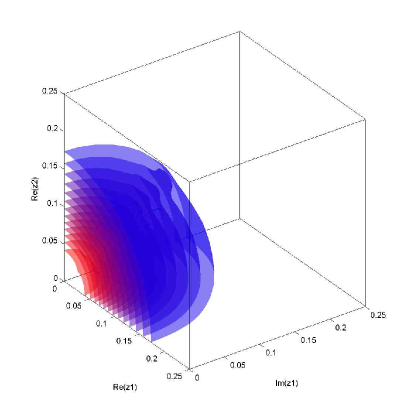
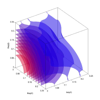
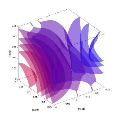
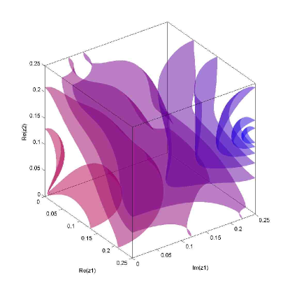
Figure 1: Isosurfaces of the Euler density $\rho$ in the $z^{i}$ coordinate system, on the $\operatorname{Im}z^{2}=0$ slice. Only the fundamental domain of the discrete symmetry group is shown, namely the cubical region $0\leq\operatorname{Re}z^{1},\operatorname{Im}z^{1},\operatorname{Re}z^{2}\leq\frac{1}{4}$ (thus the full $\operatorname{Im}z^{2}=0$ slice, which is a $T^{3}/\mathbf{Z}_{2}$, is 32 times as large as what is shown). Blue indicates lower curvature, red higher, with surfaces shown at $\rho=10^{-1.5},10^{-1},\dots,10^{4},10^{4.5}$. Left to right and top to bottom, $\alpha=0.03,0.13,0.28,0.50$.

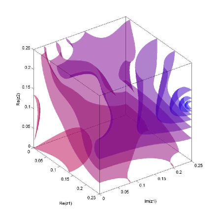
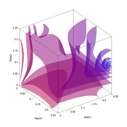
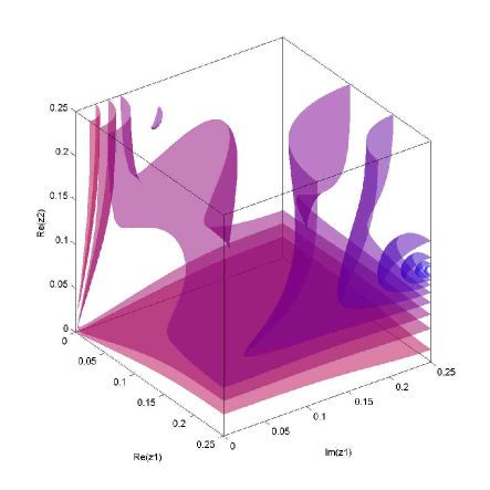
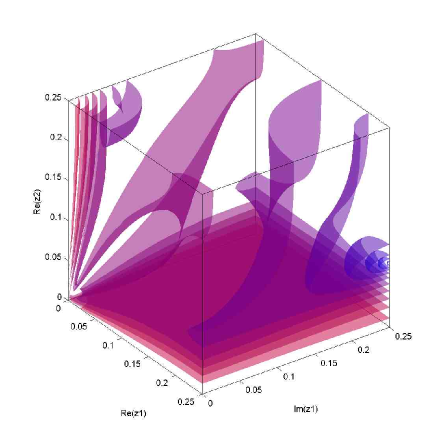
Figure 2: As in figure 1, but for $\alpha=0.61,0.72,0.85,0.92$.

On a Ricci-flat manifold, the simplest non-trivial curvature invariant one can construct is the square of the Riemann tensor (sometimes referred to as the Kretschmann invariant). In four dimensions, this happens to be proportional to the Euler density $\rho$:

$$\chi=\int\sqrt{g}\,\rho,\qquad\rho=\frac{1}{8\pi^{2}}R_{i{\bar{\jmath}}k\bar{l}}R^{i{\bar{\jmath}}k\bar{l}}.$$ (33)

Thus its integral over the manifold is fixed, in this case at 24. Figures 1 and 2 show surfaces of constant $\rho$ on the three-dimensional slice $\operatorname{Im}z^{2}=0$ at eight different values of $\alpha$. At the smallest value ($\alpha=0.03$), the curvature is highly concentrated near the fixed point, and is spherically distributed; here the metric closely approximates the Eguchi-Hanson metric (for which the isosurfaces of $\rho$ are spherical in these coordinates, although the full geometry is only axisymmetric). As we increase $\alpha$, the curvature spreads out from the fixed point. However, it does not diffuse uniformly over the manifold. Instead, starting in the $\alpha=0.72$ figure (third to last), it gathers along the $z^{1}=0$ and $z^{2}=0$ planes. These are the rational curves, discussed in the last subsection (and referred to as $\hat{c}_{1}$ and $\hat{c}_{2}$ in Appendix B), that shrink to zero size as $\alpha$ approaches 1. By symmetry, the curvature also accumulates at the 6 other shrinking rational curves, $\{z^{1}=C\}$ and $\{z^{2}=C\}$ for $C=\frac{1}{2},\frac{i}{2},\frac{1}{2}+\frac{i}{2}$.

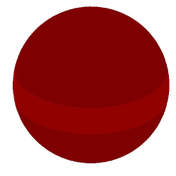
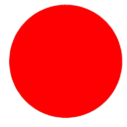
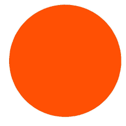
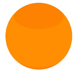
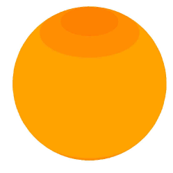
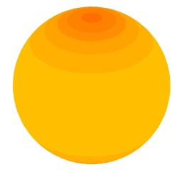
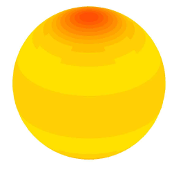
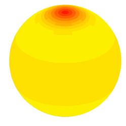
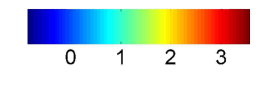
Figure 3: Log (base 10) of the Ricci scalar of the induced metric on the exceptional divisor $w=0$. Points on the sphere are mapped stereographically from their $y$ coordinate, with the north and south poles corresponding to $y=0$ and $y^{\prime}=0$. Values of $\alpha$ are as in figures 1 and 2. The average value of the Ricci scalar over the sphere decreases as its area increases, as is clear from the figure.

In the $z^{i}$ coordinate system used in figures 1 and 2, the exceptional divisor (of the original orbifold) is represented as a single point, namely the origin. This is misleading, since in fact it is topologically an $S^{2}$. It’s interesting to study how its geometry changes as we vary $\alpha$. The induced metric on the exceptional divisor of the Eguchi-Hanson geometry is that of a round sphere. We therefore expect the same to be true for the exceptional divisor of the Kummer surface at small $\alpha$. In figure 3, we plot the Ricci scalar of the induced metric on the exceptional divisor. For small values of $\alpha$, it is indeed uniform. However, as $\alpha$ increases, it becomes non-uniform (its integral is of course fixed at $8\pi$): the sphere is becoming prolate. The poles, where the curvature is highest, are at $y=0$ and $y^{\prime}=0$, in other words where the exceptional divisor intersects the planes $z^{1}=0$ and $z^{2}=0$ respectively; these are the points that are closest to neighboring exceptional divisors.

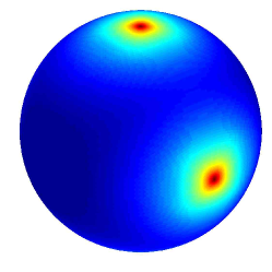
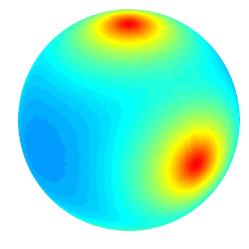
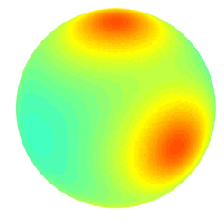
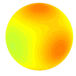
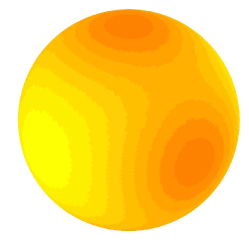
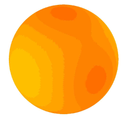
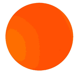
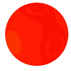
Figure 4: Log (base 10) of the Ricci scalar of the induced metric on the rational curve $\{z^{1}=0\}$. (The Ricci scalar is everywhere positive.) Using the function $\hat{y}(z^{2})=-i\wp(z^{2})/\wp(\frac{1}{2})$ (with $\wp$ the appropriate Weierstrass elliptic function), points are mapped from $T^{2}/\mathbf{Z}_{2}$ to the complex plane; $\hat{y}$ is then mapped stereographically to the sphere. The maxima of the Ricci scalar are at $z^{2}=0,\frac{1}{2},\frac{i}{2},\frac{1}{2}+\frac{i}{2}$. Values of $\alpha$ are as in figures 1 and 2. The average value of the Ricci scalar over the sphere increases as its area shrinks (see equation (30)), as is clear from the figure.

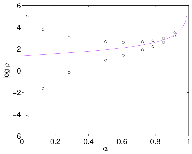
Figure 5: Maximum and minimum values of the Euler density $\rho$ on the rational curve $\{z^{1}=0\}$ as a function of $\alpha$. The solid curve is the value of $\rho$ on the exceptional divisor of an Eguchi-Hanson geometry whose exceptional divisor has area $\hat{A}$.

Similarly, it is interesting to study the induced geometry of the shrinking rational curves, for example the curve $\{z^{1}=0\}$, as shown in figure 4. At $\alpha=0$ its geometry is that of a flat $T^{2}$ orbifolded by $\mathbf{Z}_{2}$, which is topologically $S^{2}$ but with all the curvature concentrated at the 4 fixed points $z^{2}=0,\frac{1}{2},\frac{i}{2},\frac{1}{2}+\frac{i}{2}$ (picture a square envelope). As $\alpha$ increases, the curvature spreads out around the sphere, which becomes rounder and rounder. In the limit $\alpha\to 1$, the geometry in the vicinity of the shrinking rational curve should approach that of an Eguchi-Hanson metric whose exceptional divisor has area $\hat{A}=\frac{1}{2}b^{2}-2\pi a^{2}$. Indeed, we see that for values of $\alpha$ approaching 1, the sphere becomes almost completely round. As another test that the geometry is approaching Eguchi-Hanson, in figure 4 we plot the maximum and minimum values of $\rho$ on the curve against $\alpha$. On an Eguchi-Hanson, the Euler density is constant on the exceptional divisor; the solid curve in that plot is the value of $\rho$ on the exceptional divisor of an Eguchi-Hanson of the appropriate size. One sees that as $\alpha$ approaches 1 the maximum and minimum values of $\rho$ approach each other and the Eguchi-Hanson value.

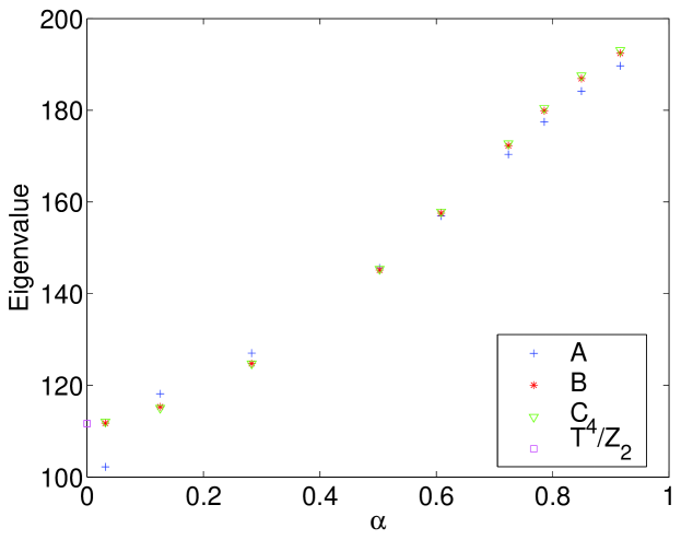
Figure 6: An eigenvalue of minus the scalar Laplacian as a function of $\alpha$. Specifically, the lowest eigenvalue whose eigenfunction is antisymmetric under all 4 generators of the $\mathbf{Z}_{2}^{4}$ translation group of the symmetric Kummer surface. A, B, and C represent increasing lattice resolutions, as detailed in Appendix A. The exact eigenvalue at the orbifold point $\alpha=0$ is also shown.

Given the Ricci-flat metric, one can compute the spectrum of various geometric operators of physical interest, the simplest example being the scalar Laplacian. As a proof of principle, we used our numerical metrics to compute a low-lying eigenvalue (and eigenfunction) of it. The eigenfunctions of the Laplacian on our symmetric Kummer surface can be classified by their eigenvalues under the $\mathbf{Z}_{2}^{4}$ translation subgroup of its full symmetry group. We calculated the lowest eigenvalue in the sector with eigenvalue $-1$ under all 4 translations. The results are shown in figure 5. The eigenvalue at the orbifold point $\alpha=0$, which can be computed exactly, is also shown for comparison. The fact that the eigenvalue increases with $\alpha$ can be understood heuristically (at least for small values of $\alpha$) in the following way. As the rational curves discussed above shrink, the geodesic distance between a point on the exceptional divisor, such as $y=w=0$, and its image under each of the discrete translations decreases, requiring steeper gradients in the eigenfunction. Finally, we would like to point out that, as we are studying a long wavelength eigenfunction, even the lowest resolution (A) computes the eigenvalues to typically within a few percent of the continuum extrapolated value.

We close this section on a technical note. Careful inspection of the isosurfaces plotted for the smallest value of $\alpha$ in figure 1 shows a localized deviation from sphericity, caused by small errors near patch overlaps. Similarly, in figure 3 the smallest $\alpha$ sphere is slightly less uniform than for the next larger value of $\alpha$; in figure 4 for the largest value of $\alpha$ we can just see some “rings” where small errors are introduced due to coordinate patch overlaps; and the distance from the extrapolated continuum values in figure 6 increases near $\alpha=0$ or $1$. Numerical discretization errors are to be expected, and will be larger where there are higher curvatures. Our solutions containing the highest curvature regions occur near the two orbifold points $\alpha=0,1$, explaining why we see the effects mentioned above. Hence, at a fixed resolution, the global quality of the solutions will not be as high near these orbifold points, although the local geometry away from the regions of high curvature should be quite acceptable. Of course, increasing the resolution, the quality of the solution will improve, independently of where we are in moduli space. These issues are discussed in more detail in appendix A.3.

4 Discussion

4.1 Generalizations

We opened this paper with the question of whether it is possible, in practice, to solve the Einstein equation numerically on a Calabi-Yau manifold. We have shown that the answer is affirmative when the Calabi-Yau is a K3 surface with a high degree of discrete symmetry. In this subsection we will investigate the possibility of generalizing this accomplishment, first to more general K3 surfaces, then to Calabi-Yau three-folds, and finally to Kähler manifolds with cosmological constant or with matter.

It is clear that in principle our method extends to a general blow-up of a Kummer surface, and more generally to any K3 surface. It is merely necessary to implement the topology and complex structure with complex coordinates defined appropriately on an atlas of charts—for example one could use patches derived from any algebraic construction of K3. However, the question remains as to what resolution is attainable in the absence of large amounts of discrete symmetry. Our highest resolution, $D$, simulated approximately $2\times 10^{7}\approx 80^{4}$ points. However, due to the high degree of discrete symmetry our one parameter family of K3’s enjoy, every computed point actually represents $2^{9}$ points in the true K3 geometry, and hence we have described the full K3 with an effective resolution of around $400^{4}$.

On a current high-end desktop computer (with 1 to 2 gigabytes of memory) one could comfortably increase the total number of points simulated to $10^{8}$. For a K3 with no discrete symmetry this would yield a resolution of $100^{4}$ for the full K3 geometry. To estimate how accuately this could represent the metric, we may compare it to our intermediate resolution, B. With a linear resolution 4 times lower than that for D, the effective resolution for the full geometry is also about $100^{4}$. As seen in subsection 3.2 and appendix A we find that resolution B adequately reproduces the geometry and derived properties, such as the low wavelength eigenmodes of the Laplace operator, provided one is not too close to the edge of the Kähler cone. For example, in figure 6 one sees that run B computed the Laplacian eigenvalue with an accuracy of around 1% compared to the extrapolated continuum value. Near the edge of the Kähler cone, where regions of high curvature develop in the manifold, the best strategy may be to combine numerical with analytic techniques. For example, at values of the moduli near an orbifold point, one could patch an analytic Ricci-flat metric, such as the Eguchi-Hanson metric, into the region where the high curvature is developing.

If we now wish to move to a Calabi-Yau three-fold, $10^{8}$ points translates to a mere 20 points linearly in each direction. This is over a factor of 2 less in linear resolution than the lowest effective resolution used in this work (run A, which had an effective resolution of $50^{4}$ for the full geometry). This might be acceptable if one were well away from the Kähler cone edge, but is certainly rather low. On the other hand, if one were to consider a highly symmetric three-fold, such as a symmetric blow-up of $T^{6}/\mathbf{Z}_{3}$, then one would again expect to attain an effective resolution of around $100$ points linearly in the full geometry, and thus again expect accuracy comparable to, or better than, our resolution B.

Moving to the general three-fold appears to be a very challenging task. As we discuss in Appendix A, processing time actually scales rather well with increasing dimension. Instead the problem is limited by storage. In six real dimensions any appreciable increase in linear resolution is extremely costly. Thus whilst $20^{6}$ points would be possible on a desktop computer, $40^{6}$ requires 64 times more memory and is already beyond the abilities of modest clusters. Often a tough computational problem becomes easy in time, as computer memory and speed have closely followed Moore’s prediction of a doubling every 2 years. However, even assuming that Moore’s law continues to hold, it will require 12 years to increase the linear resolution by a factor of 2 for the three-folds. It is therefore clear that in order to tackle the general three-fold, one must employ considerably more sophisticated discretization schemes than we have used here, presumably adapting the lattice points to regions of high curvature. Whilst adaptive grids are difficult to implement in the elliptic context, one can easily use fixed grids that increase resolution in areas where curvature is expected to be high.

To summarize, we expect that for a general K3 surface one can obtain very satisfactory results provided one does not wish to probe too near the edge of the Kähler cone. For a highly symmetric three-fold similarly high quality results can be expected. However, moving to the general three-fold appears tough and new techniques must certainly be employed.

Having considered the problem of constructing K3’s at arbitrary points in moduli space, we should point out the enormity of the moduli space itself: with 57 directions to explore it is highly implausible that one could ever map the entire space of K3’s. On the other hand it is unlikely that one would ever need to map the entire space. One can imagine wishing to find K3 surfaces with specific properties; presuming the observables of interest vary smoothly over the moduli space, it is plausible that one could scan the moduli space for examples that fit the specific requirements.

Whilst Calabi-Yau’s have large numbers of moduli, spaces with Ricci curvature tend to have fewer of them. An example of this are the four (real) dimensional del Pezzo surfaces dP_n ($n=1,\dots,8$), compact Kähler spaces that can be constructed by blowing up $n$ points in $\mathbf{C}P^{2}$. Del Pezzos have positive first Chern class, and those with $n\geq 3$ admit Kähler-Einstein metrics with no Kähler moduli. The cases of dP₃ and dP₄ are particularly interesting because they also have no complex structure moduli. The Einstein equation can again be reduced to a Monge-Ampère equation for the Kähler potential. As in our K3 example, two patches would be required to cover each of the $n$ blown up points, and three to cover the ambient $\mathbf{C}P^{2}$. Hence we expect the methods we have applied here for K3 to be applicable, and the Kähler-Einstein metrics to be attainable to high resolution on a desktop computer (certainly comparable to or better than our resolution C, depending on how many points are blown up in $\mathbf{C}P^{2}$). This would be very satisfying for dP₃ and dP₄ as, with no moduli, one would in principle have constructed these geometries explicitly and completely.

Other physically interesting geometries that are related to Calabi-Yau manifolds are supersymmetric flux compactifications in string theory. A class of type IIB solutions can be constructed as warped products of flat four-dimensional Minkowski spacetime and a Ricci-flat Calabi-Yau three-fold, where the warp factor satisfies a Poisson equation on the Calabi-Yau sourced by fluxes, D-branes, and orientifold planes (see e.g. [19, 20, 21, 22]). As we discussed above, finding the metric on a generic three-fold is probably out of reach using the methods of this paper. However, considering fluxes on K3 or a highly symmetric three-fold would likely be a manageable task. Having found the Ricci-flat metric, solving the Poisson equation on this geometry is quite simple—indeed even easier than finding eigenfunctions of the Laplacian as we did earlier in this paper. Studying the solutions to the Poisson equation on the Calabi-Yau background would provide a detailed understanding of how the fluxes backreact on the vacuum geometry, and in particular of how fluxes on adjacent cycles interact.

4.2 Lessons for solving general Euclidean geometries

The key simplification in our work has been that of Kähler geometry. What are the prospects for constructing general Euclidean geometries? Without Kählerity we require many metric components to describe the geometry, and the Einstein equation becomes complicated. Whilst this may be technically complicated, in principal one would hope that using a harmonic gauge condition would allow the system to be locally solved as an elliptic relaxation problem. Note that one could also use a gauge fixed Ricci flow, but as discussed eariler, it is more efficient to solve the elliptic Ricci flatness condition directly rather than to construct an entire flow when only the endpoint is required. In our K3 example, the complex coordinates on the coordinate patches provide exactly such a local harmonic set of coordinates. However the most challenging aspect of the problem is to understand the global issues, such as residual coordinate freedom, adaptedness of the coordinates, and moduli of the solutions.

Let us for a moment consider the problem of finding the Ricci flat metric of symmetric K3’s as we have done, but ignoring the Kähler structure and using only real geometry. We might hope to find harmonic coordinates on the various patches that make up the topology. This would require us to solve the harmonic gauge condition (essentially locally solving Laplace equations) at the same time as the Einstein equation. Presumably this full system is globally elliptic in the case of K3, although for more general geometries we should note that negative modes of the Lichnerowicz operator will exist, as occurs for the Euclidean Schwarzschild solution, and it is unclear how these would affect the situation.

Given the link between the complex coordinates of Kähler geometry and the harmonic coordinates natural for Euclidean real geometry, we can make various speculations. We saw that our complex coordinates were well adapted to the symmetric K3 geometry, and one might hope the same to be true for more general harmonic coordinates. As explained above, for the complex coordinates there are no residual holomorphic coordinate transformations; in real geometry, choosing harmonic coordinates one again expects only finitely many residual coordinate freedoms on a compact manifold. Assuming this, one might conclude from our work that we may see the complex structure moduli of the K3 arise simply from the global data required to specify the harmonic coordinates, just as we have fixed the complex structure moduli by taking particular complex coordinates on the manifold. Then for more general compact manifolds, one might plausibly associate physical moduli to global choices when constructing the harmonic coordinates (that are not simply one of the finite residual coordinate transformations).

Clearly about any Ricci flat real geometry one can always linearize metric fluctuations and then, in principle, directly determine the zero modes of the resulting Lichnerowicz operator, and hence determine all physical moduli of the solution. However, this is obviously very complicated to imagine doing in practice, and what we really wish to find is a way to include the moduli as boundary conditions in the elliptic problem as we have done in our Kähler example. Assuming our presumptions above about the complex structure moduli hold, the key remaining question is how to understand the Kähler moduli of K3 as boundary conditions, without actually making use of the Kähler structure. It might be possible to understand this in terms of the volumes of minimal representatives of the two-cycles. However, whilst for K3 this approach would work, for the Kähler-Einstein case of the del Pezzos it cannot, since the two-cycles present are not associated with any moduli; hence this approach would not work in general. Thus, finding new ways to understand the Kähler moduli and how to actually implement fixing them whilst solving the real geometry Einstein equations for K3, look to be important questions. If they can be addressed, it might allow one to understand the moduli of general real geometries, and enable explicit metrics to be found in very general Euclidean geometry-matter systems.

4.3 Applications

We now briefly discuss possible applications for the numerical construction of geometries. We consider first mathematical, then formal physical, and finally phenomenological applications.

There are various outstanding mathematical conjectures regarding the geometry of Calabi-Yau manifolds. Most notorious is the Strominger-Yau-Zaslow conjecture, that Calabi-Yaus with mirrors can be constructed as toric fibrations and that mirror symmetry acts by T-duality on the fibers [23, 24]. A related conjecture concerns mean curvature flows and special Lagrangian submanifolds in Calabi-Yau manifolds [25]. In principle these conjectures can be tested directly on any Calabi-Yau for which the Ricci-flat metric is known explicitly.

From the point of view of physics, explicit constructions of Ricci-flat Calabi-Yau metrics may help us learn more about the sigma model description of geometry. The Ricci-flat metric on K3 is the target space of an ${\cal N}=(4,4)$ non-linear sigma model. Due to the high degree of supersymmetry the classical Ricci flat metric receives no perturbative or non-perturbative corrections in $\alpha^{\prime}$ [12]. Thus the geometries we have constructed in this paper can, remarkably, be viewed as fully quantum geometries from the viewpoint of this sigma model. Knowing these metrics then in principle allows one to compute properties of the quantum sigma model—for example, the spectra of operators on the target manifold correspond to conformal weights on the worldsheet.

The Ricci-flat Calabi-Yau three-folds are again target spaces of sigma models. However, now the classical geometry only gives the leading $\alpha^{\prime}$, or large volume, approximation to the true quantum geometry. Understanding how $\alpha^{\prime}$ corrections modify the classical geometry is an important physical issue. Supersymmetry implies that these corrections preserve the Kählerity of the metric, and hence they will appear as higher derivative terms modifying the Monge-Ampère equation for the Kähler potential. Each higher derivative term will make this equation less local, but in principle we may still apply the same local iterative methods we have used here to solve it. (Presumably on a compact manifold, one could in principle include infinitely high derivative terms if their form were known.) From a discretized viewpoint, if we linearized the equation about some background, we would find an $N\times N$ operator ($N$ being the total number of lattice points) and the structure of its matrix representation will no longer be sparse. However, the terms that fill in the zero components in the sparse Monge-Ampère case will be small, being down by factors of $\alpha^{\prime}$. Hence our Gauss-Seidel iterative methods may still work, although obviously evaluation of the equation at each point will take much longer.

Finally, from a phenomenological point of view, being able to compute metrics is crucial for actually making contact with low energy physics in string theory. Whilst for simple vacuum Calabi-Yau reductions it is possible to compute the entire low energy effective action using only topological data [26], as soon as matter is added to the compactification manifold this is no longer true. The simplest example is adding a single brane that is localized in the compact space. The moduli space metric for this brane, and hence the kinetic term for its position in the low-energy action, is simply given by the metric on the internal space [27]. Thus from a physics standpoint, being able to compute the low energy action of geometric reductions is a strong motivation to further understand and improve the numerical geometry methods we are exploring here.

It is worth mentioning that in TeV fundamental scale senarios [28, 29] it is possible that in a few years the LHC might directly probe not just the low energy action, but also high energy excitations on the internal space, such as Kaluza-Klein modes. Although the LHC would likely not measure a sufficient number for any detailed spectroscopy of the internal space, future colliders would then be able to measure these massive excitations accurately. If one could extend our methods to the general three-fold—and surely this would be enough motivation to direct serious resources to it—then one might scan the moduli space of Calabi-Yaus, presumably with fluxes, to find candidate geometries matching the observed resonances.

Appendix A Details of numerical construction

A.1 Construction of the atlas and initial data

As discussed in section 3.1 our one parameter family of K3’s have many discrete symmetries. In particular these imply we may take the Kähler potential to be identical in each of the 16 regions describing the blow up of the torus fixed points. These regions are each described in terms of 2 coordinate patches given by $w,y$ and $w^{\prime},y^{\prime}$ and the symmetry $z^{1}\leftrightarrow z^{2}$ implies that the Kähler potential may be taken to be identical in each of these. Thus we reduce our problem to one patch describing the fundamental domain of the torus using $z^{1},z^{2}$ coordinates, where we orbifold by the identification $(z^{1},z^{2})\equiv(-z^{1},-z^{2})$, and one patch describing (half of) the blow up of the fixed point contained in that fundamental domain using coordinates $w,y$. We term these patches the ‘Torus patch’ and the ‘Eguchi-Hanson patch’. To begin describing the geometry of our atlas we define,

$$\sigma=|z^{1}|^{2}+|z^{2}|^{2}=2|w|\left(1+|y|^{2}\right)$$ (34)

We take our torus patch to cover the coordinate range of the fundamental domain, but exclude the region near the blown up fixed point so,

$$-\frac{1}{4}\leq\operatorname{Re}{z^{1,2}}\leq\frac{1}{4}\quad,\quad-\frac{1}{4}\leq\operatorname{Im}{z^{1,2}}\leq\frac{1}{4}\quad\mathrm{and}\quad\sigma\geq\sigma_{min}$$ (35)

Outside the boundaries of this domain we must act with the translations $z^{1,2}\rightarrow z^{1,2}\pm(1,i)/2$ to map the point back into the domain. Note that when we do this, we must also ensure we perform the torus Kähler transformation derived from 25 reduced to this domain. The Eguchi-Hanson patch is taken to have coordinate range,

$$0\leq|y|\leq y_{max}\quad\mathrm{and}\quad\sigma\leq\sigma_{max}$$ (36)

In order to cover the manifold we must ensure $y_{max}\geq 1$, and $\sigma_{max}\geq\sigma_{min}$ with $\sigma_{max}<1/4^{2}$ to avoid complicated multiple overlaps.

In order to evaluate our Monge-Ampère equation at the edge of a coordinate patch we must necessarily compute derivatives involving Kähler potential data from neighbouring coordinate patches. Once we have finite differenced our patches this will require the Kähler potential at some point to be computed from the neighbouring patch and then Kähler transformed into the original patch. The coordinate location in the neighbouring patch will not necessarily fall on a lattice point and therefore we will need to perform interpolation to compute the desired Kähler potential . Thus we require our patches to overlap sufficiently in order to perform our necessary interpolations.

For example, suppose when we evaluate a derivative at the boundary of the Eguchi-Hanson patch we require knowing the Kähler potential at a point still with $\sigma<\sigma_{max}$ but now $|y|>y_{max}$. Then we must use the coordinate patch $w^{\prime},y^{\prime}$ - which due to the discrete symmetries is identical to the $w,y$ one. Explicitly, we transform to the $w^{\prime},y^{\prime}$ coordinates where still $\sigma<\sigma_{max}$, but now $|y^{\prime}|<y_{max}$, so the point does indeed lie within this $w^{\prime},y^{\prime}$ patch. We find the Kähler potential in this patch using the necessary interpolation, and then return to our original coordinate patch $w,y$ by performing the necessary Kähler transformation 28. Similarly, at the large $\sigma$ boundary of the Eguchi-Hanson patch, or small $\sigma$ boundary of the torus patch we will find the Kähler potential in that patch by interpolating from the other and performing the appropriate Kähler transformations 26, 27.

We note that in fact we actually require only one coordinate patch, as the Eguchi-Hanson patch can quite satisfactorily represent the torus region. However, the torus patch boundary conditions, essentially derived from 22-25 become complicated and non-local in the $w,y$ coordinates, and we have found it simpler to use the two patches above, rather than the minimal choice of one patch.

Even after the reduction to these 2 patches, and the coordinate domains above, we still have discrete symmetries remaining. The orbifold symmetry, holomophic isometries $z^{j}\rightarrow iz^{j}$, $z^{1}\leftrightarrow z^{2}$ and anti-holomorphic isometry $z^{1,2}\leftrightarrow\bar{z}^{1,2}$ further reduce the torus coordinate domain (in addition to $\sigma\geq\sigma_{min}$) to,

$$0\leq\operatorname{Re}{z^{1,2}} \leq \frac{1}{4}\quad,\quad 0\leq\operatorname{Im}{z^{1,2}}\leq\frac{1}{4}$$

$$\mathrm{and}\qquad(z^{1},z^{2}) \sim (z^{2},z^{1})$$

$$(z^{1},z^{2}) \sim (\bar{z}^{1},\bar{z}^{2})$$ (37)

In the Eguchi-Hanson patch these isometries allow us to further reduce 36 to,

$$0\leq\operatorname{Re}{w,y}\qquad 0\leq\operatorname{Im}{w,y}$$ (38)

The Kähler potential does not transform under these discrete isometries, and therefore if we now require a point to be evaluated outside our reduced coordinate domains we simply use these discrete symmetries to map the point back into our reduced coordinate domain.

In the data we present we have chosen a fixed geometry for the patches and their overlaps. This is independent of the numerical resolution of the discretization so that for convergence testing we are comparing like with like. As discussed in section 2.3 it also allows us to directly compare the Kähler potential in the same overlapping regions as we vary the resolution which provides a check of numerical convergence. The parameters we have chosen are,

$$y_{max}=1.25\qquad\sigma_{min}=\frac{1}{4^{2}}\times 0.32\quad\mathrm{and}\quad\sigma_{max}=\frac{1}{4^{2}}\times 0.60$$ (39)

Before we begin relaxing the Monge-Ampère equation we require some smooth initial data compatible with our choice of Kähler parameters $a,b$ (although in fact we have found that in some cases even taking non-smooth initial data the algorithm still converges). We construct this by taking an initial guess Kähler potential to have the behaviour of the Eguchi-Hanson potential near $\sigma=0$ in the Eguchi-Hanson patch, and which then interpolates smoothly up to second derivatives to behave as the flat torus potential for $\sigma>\sigma_{max}$.

The Eguchi-Hanson potential in the coordinate patch $w,y$ is given by,

$$K^{\mathrm{EH}}_{(y,w)}=\frac{1}{2}\sqrt{\sigma^{2}+a^{4}}+\frac{a^{2}}{2}\ln\frac{\ln\left(1+|y|^{2}\right)}{1+\sqrt{1+\frac{\sigma^{2}}{a^{4}}}}$$ (40)

and the flat torus potential is simply $K^{\mathrm{torus}}=\frac{1}{2}\sigma b^{2}$. For our interpolation, in our Eguchi-Hansen patch (with $\sigma<\sigma_{max}$) we take,

$$K_{(y,w)} = \frac{1}{2}a^{2}\log{(1+|y|^{2})}+k_{0}+k_{2}\sigma^{2}+k_{4}\sigma^{4}$$

$$\mathrm{with}\qquad k_{0} = \frac{1}{16}\left(6a^{2}+3\sigma_{max}b^{2}-8a^{2}\log{\sigma_{max}}\right)$$

$$k_{2} = \frac{1}{8\sigma_{max}^{2}}\left(3\sigma_{max}b^{2}-4a^{2}\right)$$

$$k_{4} = -\frac{1}{16\sigma_{max}^{4}}\left(\sigma_{max}b^{2}-2a^{2}\right)$$

and in the torus patch with $\sigma>\sigma_{min}$ we take,

$$\sigma\leq\sigma_{max}\qquad K_{(z1,z2)} = \frac{1}{2}a^{2}\log{\sigma}+k_{0}+k_{2}\sigma^{2}+k_{4}\sigma^{4}$$

$$\sigma>\sigma_{max}\qquad K_{(z1,z2)} = \frac{1}{2}\sigma b^{2}$$

The constants above ensure the Kähler potential has smooth second derivatives at $\sigma=\sigma_{max}$. However, it is easy to show that the above does not define a positive Kähler form over the whole range $\alpha=0$ to $1$. As discussed in the main text, one advantage in solving the Monge-Ampére equation directly, rather than performing Ricci flow, is that the Kähler form need not be positive. Hence the simple interpolation above suffices as initial data.

A.2 Discretization, memory and time requirements

We discretize our system in the most naive way. In both patches we discretize by creating a uniform lattice in the real and imaginary parts of each complex coordinate. We then use second order finite differencing to implement the Monge-Ampére equation and third order accurate interpolation at the patch overlaps.

At each step of our relaxation, we firstly interpolate the values of the Kähler potential at the very edges of a patch from the appropriate neighbouring patches, and secondly perform one iteration of the Gauss-Seidel generalizated to our Monge-Ampère equation. When updating each point, as a by-product we may quickly compute the value of $\det{g}$ at that point. During the Gauss-Siedel update, we keep a running average of this quantity over all lattice points, and then use this as the value of $\tilde{\lambda}$ for the next step. This ensures our Gauss-Seidel iterations asymptote to a fixed solution.

In this paper we have used 4 different resolutions each differing in linear resolution by a factor of 2. In the the torus patch we discretize with equal lattice spacing $dz$ in the real and imaginary $z^{1}$ and $z^{2}$ directions. In the Eguchi-Hanson patch we discretize with spacing $dw$ in the real/imaginary $w$ directions and $dy$ in the real/imaginary $y$ directions. We label the various resolutions $A-D$, and they are specified as,

$$\begin{array}[]{rclrclrcl}A\qquad\qquad dz&=&0.025&dw&=&0.003125&dy&=&0.25\\ B\qquad\qquad dz&=&\frac{1}{2}0.025&dw&=&\frac{1}{2}0.003125&dy&=&\frac{1}{2}0.25\\ C\qquad\qquad dz&=&\frac{1}{2^{2}}0.025&dw&=&\frac{1}{2^{2}}0.003125&dy&=&\frac{1}{2^{2}}0.25\\ D\qquad\qquad dz&=&\frac{1}{2^{3}}0.025&dw&=&\frac{1}{2^{3}}0.003125&dy&=&\frac{1}{2^{3}}0.25\\ \end{array}$$ (43)

Remembering that the coordinates $z$ range from $0\rightarrow 0.25$ for our reduced domain in the torus patch, this yields 80 points along a side of the torus in resolution $D$.

In the torus patch we implement the 2 identifications in A.1 imperfectly by simply only storing points with $\operatorname{Im}(z^{2})>\max{\left(\operatorname{Re}(z^{1}),\operatorname{Im}(z^{1})\right)}$. This is rather convenient, but doesn’t fully take advantage of these discrete symmetries. Asymptotically this yields a reduction of 3 rather than the optimal value 4 for these 2 identifications. With this minor imperfections in mind, the total number of points stored in computer memory for each resolution to represent the manifold is then,

$$\begin{array}[]{rcl}\mbox{number of points}\quad A&=&6\times 10^{3}\\ B&=&7\times 10^{4}\\ C&=&1\times 10^{6}\\ D&=&2\times 10^{7}\\ \end{array}$$ (44)

The Gauss-Seidel scheme is implemented by solving the discrete Monge-Ampère equations at each point in the lattice. We found that under-relaxation was not required for stability and the scheme converged stably. Interestingly we found that we could not over-relax the equation with any appreciable over-relaxation rendering the scheme unstable. Presumably this is an effect associated with the patch boundaries rather than their interiors which we expect to behave in an analogous manner to the Poisson equation. Thus in principle it might be possible to include an over-relaxation parameter that varied over the patch to be one at the edges, but larger than one in the interior.

We measure the distance from convergence by computing the maximum update of the Kähler potential in a given Gauss-Seidel iteration over the whole lattice. This is equivalent to computing the maximum violation of the discretized Monge-Ampère equation.

When this number falls below $10^{-12}$ we classify the solution as having relaxed. Certainly for any quantity we have computed, there is no further change if the solutions are subjected to further iterations of the Gauss-Seidel scheme. The time taken for our implementation of the algorithm from initial guess to the relaxed condition is shown in figure 7 for the various resolutions $A-D$ on a standard desktop computer (3Ghz Pentium, 500 Mb). After a little relaxation, as for the Poisson equation, the number of Gauss-Seidel iterations required to improve the discretized error by a factor of 10 quickly tends to a constant. This is also shown in the same figure.

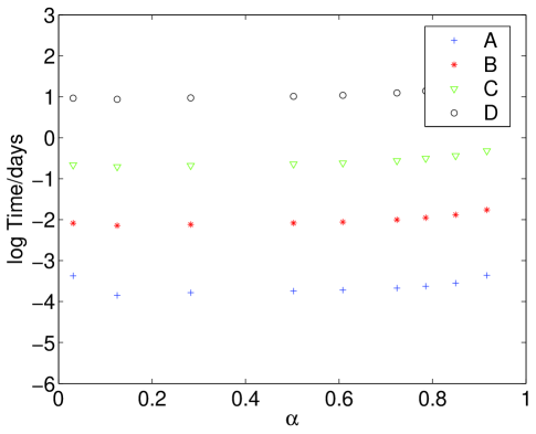
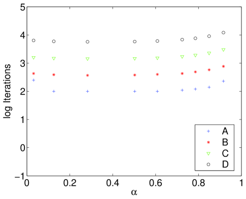
Figure 7: The lefthand plot shows the log (base 10) total time measured in days for the various resolutions $A-D$ to converge to our required degree. The righthand plot shows the number of Gauss-Seidel iterations to improve the maximum error in the discretized Monge-Ampère equation by a factor of 10.

We see that both these quantities exhibit only a weak dependence on the position in moduli space that we choose. The lowest resolution $A$ relaxes in seconds while our highest resolution $D$ requires up to a week.

The time taken to relax using the local Gauss-Seidel scheme can be estimated as going as $N^{1+2/d}$ in $d$ real dimensions where $N$ is the total number of lattice points. Every iteration takes a time of order $N$, and the total number of steps can be estimated as $N^{2/d}$ by considering the spectral radius of the linearized Laplace operator. We see this scaling is certainly consistent with the results of figure 7.

At every step in the iteration we must also perform an interpolation of points at the edge of each coordinate patch from its neighbours. We only require the edge points to be interpolated that are required by our second order differenced Monge-Ampère equation. Thus the work involved scales as a codimension one quantity, namely as $N^{(d-1)/d}$. In practice our third order interpolation actually takes considerable time. Asymptotically at large $N$, however, it will obviously become subdominant to the Gauss-Seidel iteration time which scales as $N$.

It is very interesting to note that as we move to higher dimensions, the total relaxation time more and more closely approaches $N$. Thus the advantage in using highly non-local schemes such as multi-grid to improve convergence times (typically to $N\log{N}$) becomes considerably reduced. In this sense we may claim that the problem of extending our methods to Calabi-Yau 3-folds is storage limited rather than speed limited.

In a memory limited problem, it is rather natural to move to higher order methods. Our implementation uses second order finite differencing on the Monge-Ampére equation. However, we might hope for improved convergence to the continuum if we were to use $4^{th}$ order discretization of the Monge-Ampère equation (and also for interpolating between patches). We did try this in our case of K3, but the additional time required by each iteration slowed the total convergence time to approximately the same as the next higher resolution using second order differencing. In order to procede to our highest resolution we decided to stay with second order differencing. Bear in mind that whilst a higher order method approaches the continuum more quickly, in order to resolve short length scales one requires high resolutions, so to get accurate results near the orbifold regions of our moduli space, we require the highest resolutions possible.

With a particular physics or maths question in mind, one might attempt computations using more resources and improved stamina than we have used here. Then the fundamental problem of limited storage should probably be tackled by both a combination of more efficient discretization, and also higher order methods. The increased cost in processor time could certainly be ameliorated by some form of parallelisation - which is well suited to this problem which, afterall, naturally divides into coordinate patches.

The eigenfunction of the scalar Laplace operator presented in section 3.2 was computed using a naive iterative scheme. The initial guess for the eigenfunction $\psi_{(\alpha)}$ with odd parity under the $Z_{2}^{4}$ translation isometry ($z^{i}\rightarrow z^{i}\pm 1/2$) was taken to be that for the torus orbifold, $\alpha=0$, where,

$$\psi_{(0)}=\cos{2\pi\operatorname{Re}z^{1}}\cos{2\pi\operatorname{Im}z^{1}}\cos{2\pi\operatorname{Re}z^{2}}\cos{2\pi\operatorname{Im}z^{2}}$$ (45)

giving an eigenvalue $4(2\pi/b)^{4}$. The eigenvalue equation was solved using Gauss-Seidel iteration everywhere but at one point, with the eigenvalue being determined dynamically from the condition that the eigenfunction be smooth at that point. Of course, explicit independence of the actual point chosen was checked. This method is very simple to implement, but is really only suited to finding the lowest eigenfunction in a parity sector. More sophisticated (but standard) methods would be required to computer higher eigenfunctions.

A.3 Convergence tests

We now breifly present data that demonstrates increasing numerical resolution improves observed quantities in a manner consistent with a second order approach to the continuum.

Firstly as discussed in the main text, we compute a numerical $\tilde{\lambda}$ rather than using the analytic value $\lambda$. This ensures the numerical Monge-Ampère equations converges to a static end point. We may then compare this numerical determination of $\lambda$ with the true analytic value. In figure 8 we plot the difference between these values for the various resolutions as a function of position in moduli space. We see the error is greatest near the orbifold point at $\alpha=1$ as expected. We clearly see that the errors improve with increasing resolution consistent with second order scaling - we remind the reader that the 4 resolutions $A-D$ each differ by a linear resolution factor of 2.

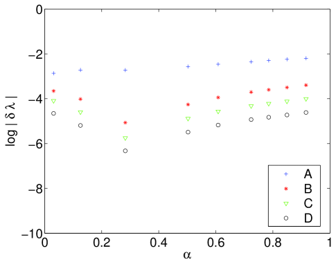
Figure 8: Plot of the log (base 10) absolute difference between the numerically determined $\tilde{\lambda}$ and the true analytic value $\lambda$ for the various resolutions $A-D$.

In figure 9 we plot the integrated Euler density for the resolutions $B-D$. The result, the Euler number, has true value 24. We clearly see here that increasing resolution does indeed improve the numerical determination of this quantity as we would hope for. The lowest resolution gives a very poor estimate of the Euler number and we have not included it here. Resolution $B$ still provides a rather poor estimate. We see the error in the Euler number is practically quite small for resolution $C$ provided we are not too near either orbifold point, and resolution $D$ gives errors of less than $0.1\%$ over most of the moduli space.

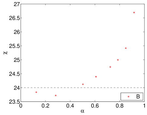
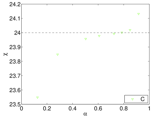
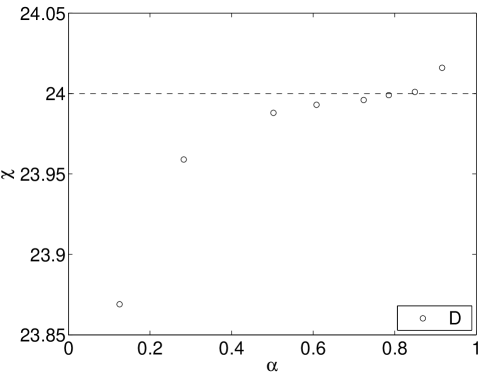
Figure 9: The Euler number integrated from the Euler density for the resolutions $B$, $C$, $D$.

Finally our patches geometrically overlap in coordinate space. Therefore as discussed in the main text, once we have found a solution, we can test its quality by computing the error in the Kähler potential in the overlapping regions (obviously taking into account the relevent Kähler transformation between the 2 patches). In figure 10 we show the maximum error found by comparing 2 different patch overlaps; the overlap of the Eguchi-Hanson patch with itself, and then its overlap with the torus patch. We see that this maximum error again decreases consistent with second order scaling as resolution is increased.

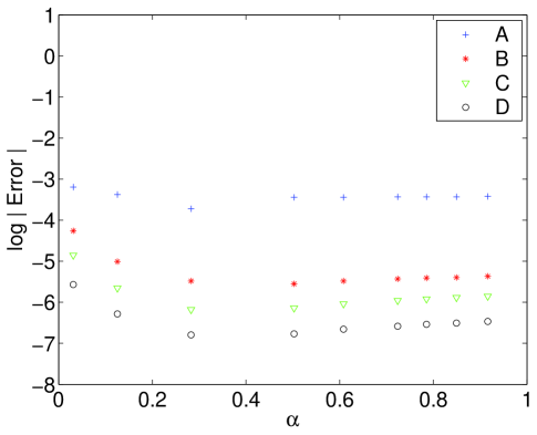
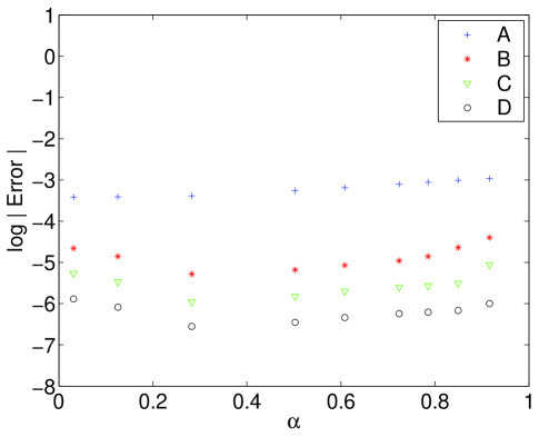
Figure 10: Lefthand plot shows the log (base 10) absolute maximum error between Kähler potentials on the overlap of the Eguchi-Hanson patch with itself. The righthand plot shows the maximum error on the overlap between the Eguchi-Hanson and torus patches.

Appendix B Homology of Kummer surfaces

In this appendix we derive some properties of the second homology group of Kummer surfaces that were used in the main text. We also show how to relate the natural basis for the homology to the standard basis for the integral homology of K3. As far as we know this explicit relation is new.

K3 has second Betti number $b_{2}=22$. In the Kummer construction, 6 two-cycles are inherited from $T^{4}$, and the other 16 are the exceptional divisors at the blown up fixed points. The second homology of $T^{4}$ is generated by the 2 holomorphic curves $\{z^{1}=C\}$ and $\{z^{2}=C\}$, as well as the 4 non-holomorphic curves $\{\operatorname{Re}z^{1}=C^{1},\operatorname{Re}z^{2}=C^{2}\}$, $\{\operatorname{Re}z^{1}=C^{1},\operatorname{Im}z^{2}=C^{2}\}$, $\{\operatorname{Im}z^{1}=C^{1},\operatorname{Re}z^{2}=C^{2}\}$, and $\{\operatorname{Im}z^{1}=C^{1},\operatorname{Im}z^{2}=C^{2}\}$. When taking the orbifold, one may choose the constant(s) in a such a way that the curve either passes through or avoids the fixed points (e.g. the holomorphic curves pass through four fixed points if $C=0$ but avoids them if $C=1/4$). In the latter case, one must include the image under the orbifold, e.g. $\{z^{1}=C\}\cup\{z^{1}=-C\}$, to obtain a two-cycle in the orbifold. (The cycles that pass through the fixed points are linear combinations of those that don’t and the exceptional divisors.) For our purposes, it is simplest to take as a basis the 6 cycles that avoid the fixed points, which we will refer to as “torus cycles”, along with the 16 exceptional divisors. We refer to these cycles as $c_{I}$, where $c_{1,2}$ are the holomorphic torus cycles, $c_{3,4,5,6}$ are the non-holomorphic torus cycles, and $c_{7,\dots,22}$ are the exceptional divisors (which are holomorphic).

It is straightforward to write down the intersection matrix in this basis. The torus cycles intersect each other in pairs, with intersection number 2. For example $c_{1}$ intersects $c_{2}$ at two points, $(C,C)$, and $(C,-C)$ (of course we don’t count $(-C,-C)$ and $(-C,C)$ separately). By construction, none of the torus cycles intersect the exceptional divisors. The latter do not intersect each other, but have self-intersection $-2$ (since they are topologically $\mathbf{C}P^{1}$’s). All in all, we find the following block diagonal intersection matrix:

$$h_{IJ}=\#(c_{I},c_{J})=2\begin{bmatrix}U&&&\\ &U&&\\ &&U&\\ &&&-I_{16}&\end{bmatrix},\qquad U=\begin{bmatrix}0&1\\ 1&0\end{bmatrix}.$$ (46)

From the Kähler transformations (22–28) the periods of the Kähler form $j_{I}=\int_{c_{I}}J$ may be computed for the symmetric Kummer surfaces:

$$j_{I}=\begin{cases}b^{2},&I=1,2\\ 0,&I=3,4,5,6\\ \pi a^{2},&I=7,\dots,22\end{cases}.$$ (47)

In the case of the holomorphic curves ($I=1,2,7,\dots,22$) these periods are their areas. In terms of the periods the volume is

$$V=\frac{1}{2}\int J\wedge J=\frac{1}{2}h^{IJ}j_{I}j_{J}=\frac{1}{2}b^{4}-4\pi^{2}a^{4},$$ (48)

where $h^{IJ}$ is the inverse intersection matrix,

$$h^{IJ}=\frac{1}{2}\begin{bmatrix}U&&&\\ &U&&\\ &&U&\\ &&&-I_{16}&\end{bmatrix}.$$ (49)

Consider now the holomorphic curve $\hat{c}_{1}=\{z^{1}=0\}$. This intersects $c_{2}$ at one point, $(0,C)$, but none of the other torus cycles. It also intersects, at one point each, 4 of the exceptional divisors, namely those located at $(0,0)$, $(0,\frac{1}{2})$, $(0,\frac{i}{2})$, $(0,\frac{1}{2}+\frac{i}{2})$, which we will call $c_{7,8,9,10}$. Using the intersection matrix, we have

$$\hat{c}_{1}=\frac{1}{2}\left(c_{1}-c_{7}-c_{8}-c_{9}-c_{10}\right).$$ (50)

Hence the area of this curve is

$$\hat{A}=\int_{\hat{c}_{1}}J=\frac{1}{2}\left(j_{1}-j_{7}-j_{8}-j_{9}-j_{10}\right)=\frac{1}{2}b^{2}-2\pi a^{2},$$ (51)

as claimed in subsection 3.1.

Now let us return to the general Kummer surface. The two-cycles $c_{I}$ are obviously integral. However, since the inverse intersection matrix (49) is not composed of integers, they do not form a basis for the integral homology $H_{2}(\text{K3},\mathbf{Z})$, but only a sublattice of it. The standard basis $\{c^{\prime}_{M}\}$ for $H_{2}(\text{K3},\mathbf{Z})$ is defined to have intersection matrix

$$h^{\prime}_{MN}=\#(c^{\prime}_{M},c^{\prime}_{N})=\begin{bmatrix}U&&&&\\ &U&&&\\ &&U&&\\ &&&-E_{8}&\\ &&&&-E_{8}\end{bmatrix},$$ (52)

where $E_{8}$ represents the Cartan matrix of that group,

$$-E_{8}=\begin{bmatrix}-2&1&&&&&&\\ 1&-2&1&&&&&\\ &1&-2&1&&&&\\ &&1&-2&1&&&\\ &&&1&-2&1&1&\\ &&&&1&-2&&\\ &&&&1&&-2&1\\ &&&&&&1&-2\end{bmatrix}.$$ (53)

The change of basis relating the $\{c_{I}\}$ to the $\{c^{\prime}_{M}\}$ is as follows:

$$c^{\prime}_{M}={M_{M}}^{I}c_{I},$$ (54)

where

$$2{M_{M}}^{I}=\\ \left[\begin{array}[]{cccccccccccccccccccccc}40&20&11&2&-14&0&-13&4&-8&-1&-8&1&11&-20&-20&-20&2&0&0&0&0&2\\ 46&23&11&2&-15&0&-14&4&-10&0&-9&1&13&-23&-22&-24&2&0&0&0&0&2\\ 8&4&0&0&0&0&-2&0&-2&0&-2&0&2&-4&-4&-4&0&0&0&0&0&0\\ 6&3&-1&-1&0&0&-1&0&-1&1&-1&-1&2&-3&-3&-3&-1&0&1&0&0&0\\ 0&0&0&0&2&0&0&0&0&0&0&0&0&0&0&0&0&0&0&0&0&0\\ -2&-1&1&1&1&1&1&0&0&-1&0&0&-1&1&1&1&0&0&-1&0&0&1\\ -4&-1&0&0&1&0&1&1&0&0&0&0&-1&1&2&2&0&0&0&0&0&0\\ 0&-1&1&0&-1&0&0&0&0&0&1&1&-1&1&0&0&0&0&0&0&0&0\\ 4&2&-1&0&0&0&-1&0&0&1&-2&-1&1&-2&-2&-2&0&0&0&0&0&0\\ 2&1&1&0&1&0&0&0&-1&-1&0&0&1&-1&-1&-1&0&0&0&0&-1&1\\ 0&0&0&0&0&0&0&0&0&0&0&0&0&0&0&0&0&0&0&0&2&0\\ 14&7&3&0&-5&0&-4&1&-3&0&-3&0&4&-7&-7&-7&0&0&0&0&-1&-1\\ -22&-11&-5&0&5&0&6&-1&5&0&5&0&-6&11&11&11&0&0&0&0&-1&-1\\ -7&-3&-2&-1&3&0&2&-2&1&1&1&0&-2&3&3&4&-1&0&0&0&0&0\\ 2&1&0&0&-1&0&0&0&0&0&-1&1&1&-1&-1&-1&0&0&1&-1&0&0\\ 0&0&0&0&0&0&0&0&0&0&0&0&0&0&0&0&0&0&0&2&0&0\\ -4&-2&1&0&0&0&1&0&1&0&1&0&-1&2&2&2&1&-1&-1&-1&0&0\\ 0&0&0&0&0&0&0&0&0&0&0&0&0&0&0&0&0&2&0&0&0&0\\ 2&1&-1&0&1&0&0&0&0&0&0&0&0&-2&-1&-1&-1&-1&0&0&0&0\\ -2&0&0&0&0&0&0&0&0&0&0&0&0&2&0&0&0&0&0&0&0&0\\ -2&-2&0&0&0&0&0&0&0&0&0&0&0&2&2&2&0&0&0&0&0&0\\ -15&-7&-4&-1&5&0&5&-2&3&0&3&-1&-5&7&7&7&0&0&1&0&0&-1\end{array}\right].$$ (55)

(Thus one has $h^{\prime}_{MN}={M_{M}}^{I}{M_{N}}^{J}h_{IJ}$.) In deriving this change of basis we made use of results in [13]. To our knowledge its explicit form is new.

References

- [1] S.-T. Yau, Calabi’s conjecture and some new results in algebraic geometry, Proc. Nat. Acad. Sci. 74 (1977) 1798–1799.
- [2] E. Calabi, On Kähler manifolds with vanishing canonical class, in Algebraic geometry and topology. A symposium in honor of S. Lefschetz, pp. 78–89. Princeton University Press, Princeton, N. J., 1957.
- [3] P. Candelas, G. T. Horowitz, A. Strominger, and E. Witten, Vacuum configurations for superstrings, Nucl. Phys. B258 (1985) 46–74.
- [4] D. Morrison. private communication (2004).
- [5] H. D. Cao, Deformation of Kähler metrics to Kähler-Einstein metrics on compact Kähler manifolds, Invent. Math. 81 (1985), no. 2 359–372.
- [6] P. Candelas, Lectures on complex manifolds, . IN *TRIESTE 1987, PROCEEDINGS, SUPERSTRINGS ’87* 1-88.
- [7] B. Chow and D. Knopf, The Ricci flow: an introduction, vol. 110 of Mathematical Surveys and Monographs. American Mathematical Society, Providence, RI, 2004.
- [8] S.-C. Chang, B. Chow, and S.-C. Chu, eds., Geometric evolution equations, vol. 367 of Contemporary Mathematics, (Providence, RI), American Mathematical Society, 2005.
- [9] D. Garfinkle and J. Isenberg, Critical behavior in Ricci flow, math.dg/0306129.
- [10] J. H. Rubinstein and R. Sinclair, Visualizing Ricci flow of manifolds of revolution, math.dg/0406189.
- [11] D. Garfinkle and J. Isenberg, Numerical studies of the behavior of Ricci flow, in Geometric evolution equations, vol. 367 of Contemp. Math., pp. 103–114. Amer. Math. Soc., Providence, RI, 2005.
- [12] P. S. Aspinwall, K3 surfaces and string duality, hep-th/9611137.
- [13] W. Nahm and K. Wendland, A hiker’s guide to K3: Aspects of N = (4,4) superconformal field theory with central charge c = 6, Commun. Math. Phys. 216 (2001) 85–138, [hep-th/9912067].
- [14] H. Inose, On certain Kummer surfaces which can be realized as non-singular quartic surfaces in , J. Fac. Sci. Univ. Tokyo Sect. IA Math. 23 (1976), no. 3 545–560.
- [15] K. Wendland. private communication (2005).
- [16] K. Wendland, On superconformal field theories associated to very attractive quartics, hep-th/0307066.
- [17] G. W. Gibbons and C. N. Pope, The positive action conjecture and asymptotically euclidean metrics in quantum gravity, Commun. Math. Phys. 66 (1979) 267–290.
- [18] Y. D. Bozhkov, A construction of almost anti-self-dual connections on Kummer surfaces, Serdica 14 (1988), no. 3 283–290.
- [19] B. de Wit, D. J. Smit, and N. D. Hari Dass, Residual supersymmetry of compactified d = 10 supergravity, Nucl. Phys. B283 (1987) 165.
- [20] B. R. Greene, K. Schalm, and G. Shiu, Warped compactifications in M and F theory, Nucl. Phys. B584 (2000) 480–508, [hep-th/0004103].
- [21] S. B. Giddings, S. Kachru, and J. Polchinski, Hierarchies from fluxes in string compactifications, Phys. Rev. D66 (2002) 106006, [hep-th/0105097].
- [22] A. R. Frey, Warped strings: Self-dual flux and contemporary compactifications, hep-th/0308156.
- [23] A. Strominger, S.-T. Yau, and E. Zaslow, Mirror symmetry is T-duality, Nucl. Phys. B479 (1996) 243–259, [hep-th/9606040].
- [24] D. R. Morrison, The geometry underlying mirror symmetry, in New trends in algebraic geometry (Warwick, 1996), vol. 264 of London Math. Soc. Lecture Note Ser., pp. 283–310. Cambridge Univ. Press, Cambridge, 1999.
- [25] R. P. Thomas and S.-T. Yau, Special Lagrangians, stable bundles and mean curvature flow, Comm. Anal. Geom. 10 (2002), no. 5 1075–1113.
- [26] A. Strominger, Yukawa couplings in superstring compactification, Phys. Rev. Lett. 55 (1985) 2547.
- [27] M. R. Douglas, Two lectures on d-geometry and noncommutative geometry, hep-th/9901146.
- [28] N. Arkani-Hamed, S. Dimopoulos, and G. R. Dvali, The hierarchy problem and new dimensions at a millimeter, Phys. Lett. B429 (1998) 263–272, [hep-ph/9803315].
- [29] I. Antoniadis, N. Arkani-Hamed, S. Dimopoulos, and G. R. Dvali, New dimensions at a millimeter to a fermi and superstrings at a TeV, Phys. Lett. B436 (1998) 257–263, [hep-ph/9804398].