ITFA-2005-20

hep-th/0506123

Positivity of energy for asymptotically locally AdS spacetimes

Miranda C.N. Cheng and Kostas Skenderis

Instituut voor Theoretische Fysica, Universiteit van Amsterdam, Valckenierstraat 65, 1018 XE Amsterdam, The Netherlands

ABSTRACT

We derive necessary conditions for the spinorial Witten-Nester energy to be well-defined for asymptotically locally AdS spacetimes. We find that the conformal boundary should admit a spinor satisfying certain differential conditions and in odd dimensions the boundary metric should be conformally Einstein. We show that these conditions are satisfied by asymptotically AdS spacetimes. The gravitational energy (obtained using the holographic stress energy tensor) and the spinorial energy are equal in even dimensions and differ by a bounded quantity related to the conformal anomaly in odd dimensions.
 mcheng,skenderi@science.uva.nl

1 Introduction

The AdS/CFT duality relates gravity in asymptotically AdS spacetimes to a quantum field theory on its conformal boundary. One of the main features of the duality is that the boundary fields parametrizing the boundary conditions of bulk fields are identified with QFT sources that couple to gauge invariant operators. In particular, the boundary metric $g_{(0)}$ is considered as a source of the boundary energy momentum tensor and at the same time is the metric of the spacetime on which the dual field theory is defined.

In quantum field theory the sources are unconstrained, so that one can functionally differentiate w.r.t. them to obtain correlation functions. Thus the duality requires the existence of spacetimes associated with general Dirichlet boundary conditions for the metric. Such general boundary conditions go beyond what has been considered in the GR literature where asymptotically AdS spacetimes (AAdS) were defined to have a specific asymptotic conformal structure, namely that of the exact AdS solution [1, 2], but they have been considered in the mathematics literature [3]. The asymptotic structure of these more general spacetimes is only locally that of AdS; we will call them asymptotically locally AdS (AlAdS) spacetimes.

An integral part of the correspondence is how conserved charges are mapped from one side to the other. This is in fact dictated by the basic AdS/CFT dictionary. On the field theory side, conserved charges are generated by conserved currents. In particular, the energy can be computed from the energy momentum tensor. Applying the AdS/CFT dictionary, we find that one should be able to compute the gravitational energy from the energy momentum tensor obtained by varying the on-shell gravitational action w.r.t. the boundary metric. Such a definition of conserved charges is available in the literature [4], but the naive implementation of this idea gives infinite answers, essentially due to the infinite volume of spacetime. In the GR literature such infinities are (explicitly or implicitly) dealt with by background subtraction. The AdS/CFT correspondence, however, suggests a new approach: one subtracts the infinities by means of boundary counterterms [5]-[16], as done in QFT in the process of renormalization. This procedure, called holographic renormalization, is by now a well studied method. We will call the charges defined using the holographic energy momentum tensor “holographic charges”. Notice that these charges are defined intrinsically rather than relative to some other spacetime. This is a definite advance over the background subtraction method, since a suitable reference spacetime does not exist in general.

The holographic charges agree with previous definitions of conserved charges [17, 1, 2, 18] when the latter are applicable, i.e. when the spacetime approaches that of the exact AdS solution and one considers the energy relative to AdS, see [19] for a detailed comparison between different definitions of conserved charges. The new definition on the other hand extends to arbitrary asymptotically locally AdS spacetimes. Moreover it was proved in [16] that these charges arise as Noether charges associated to asymptotic symmetries of such spacetimes and also shown to agree with the charges defined in the covariant phase space approach of Wald et al [20].

AAdS spacetimes are known to have positive mass relative to the AdS solution, which saturates the bound in a positive mass theorem [21]. The proof in [21] generalizes Witten’s spinorial positive energy theorem [22] for asymptotically flat spacetimes. A natural question to ask is whether the holographic energy of $AlAdS$ spacetimes is subjected to a positivity theorem. Such a generalization is far from obvious and is known to be false for asymptotically locally flat spacetimes [23, 24]. A new positivity theorem for a specific class of AlAdS spacetimes has been conjectured in [25]. In this reference an $AlAdS$ solution with negative mass (relative to AdS with periodic identification) was found but it was conjectured to be the lowest energy solution among all solutions with the same asymptotics.

Notice that the positivity of the gravitational energy implies via the AdS/CFT correspondence the positivity of the quantum QFT Hamiltonian at strong coupling. This is a very strong conclusion since for a general AlAdS the dual QFT resides on a curved manifold, and in general even the very definition of a QFT on a curved manifold is subtle. Therefore, in general we expect that only a subclass of AlAdS spacetimes is subject to a positivity theorem. One might in fact turn things around and view our discussions as giving a criterion for the selection of good boundary conditions.

This paper is organized as follows. In the next section we discuss the definition of asymptotically locally AdS spacetimes and in section 3 the definition of energy for such spacetimes. The spinorial energy of Witten and Nester is reviewed in section 4. In section 5, we construct asymptotic solutions of the Witten equation and use them in section 6 to compute a regulated version of the Witten-Nester energy for AlAdS spacetimes. This leads to a number of necessary conditions for the existence of such an energy. In section 7 we compare the finite part of the Witten-Nester energy with the holographic energy. In section 8 we specialize to AAdS spacetimes and in section 9 we illustrate subtleties related to some global issues by discussing two examples, the extremal BTZ black hole and the AdS soliton. We conclude with a discussion of our results in section 10. In order to keep the line of argument clear, we have moved most of the technical details to a series of appendices.

2 Asymptotically locally AdS spacetimes

We discuss in this section the definition of asymptotically locally anti-de Sitter (AlAdS) spacetimes. More details can be found in [13, 16] and the mathematics reviews [26, 27]. In this paper, we restrict our attention to the case of pure gravity but the method can be generalized to include matter.

The most general asymptotic solution of Einstein’s equations with negative cosmological constant takes the form [3]

$$ds^{2}=G_{\mu\nu}dx^{\mu}dx^{\nu}=\frac{dz^{2}}{z^{2}}+\frac{1}{z^{2}}g_{ij}(x,z)dx^{i}dx^{j},$$

$$g(x,z)=g_{(0)}+zg_{(1)}\cdots+z^{d}g_{(d)}+h_{(d)}z^{d}\log z^{2}+\cdots$$ (2.1)

In these coordinates $z=0$ is the location of the conformal boundary of spacetime and $g_{(0)}$ is an arbitrary non-degenerate metric (which represents the conformal structure of the boundary). Einstein equations determine uniquely all coefficients in (2) except for the transverse traceless part of $g_{(d)}$ [3, 5, 8] (see appendix A of [8] for concrete expressions). A short computation reveals that the Riemann tensor of the metric (2) is asymptotically equal to

$$R_{\mu\nu\kappa\lambda}=(G_{\mu\lambda}G_{\nu\kappa}-G_{\kappa\mu}G_{\nu\lambda})(1+{\cal O}(z))$$ (2.2)

where the cosmological constant is normalized as $\Lambda=-d(d-1)/2$ (i.e. we set the AdS radius equal to one). Thus the leading form of the Riemann tensor is exactly the same as the Riemann tensor of the $AdS_{d+1}$ spacetime. We will call solutions with this property “asymptotically locally AdS” (AlAdS) spacetimes. All solutions of pure gravity with negative cosmological constant are of this form. Notice that we do not require the conformal structure of (2) to be that of $AdS_{d+1}$. Spacetimes with this conformal structure are called “asymptotically AdS” [1, 2].

Recall that $AdS_{d+1}$ is conformally flat and this implies [28] that $g_{(0)}$ is also conformally flat and the expansion (2) terminates at order $z^{4}$,

$$g(x,z)=\left(1+\frac{z^{2}}{2}g_{(2)}g_{(0)}^{-1}\right)g_{(0)}\left(1+\frac{z^{2}}{2}g_{(0)}^{-1}g_{(2)}\right)$$ (2.3)

with

$$d=2:\qquad g_{(2)ij} = -\frac{1}{2}(Rg_{(0)ij}+t_{ij}),\qquad\nabla^{i}t_{ij}=0,\quad t^{i}_{i}=R,$$ (2.4)

$$d\neq 2:\qquad g_{(2)ij} = -\frac{1}{d-2}(R_{ij}-\frac{1}{2(d-1)}Rg_{(0)ij}),$$

where $R_{ij}$ is the Ricci tensor of $g_{(0)}$ and the transverse traceless part of $t_{ij}$ is not determined by the asymptotic analysis. $g_{(0)}$ may be chosen to be the standard metric $\mathbf{R}\times S^{d-1}$. By definition, $AAdS_{d+1}$ spacetimes have the same boundary conformal structure as $AdS_{d+1}$. This implies that all coefficients up to $g_{(d)}$ are the same as those for $AdS_{d+1}$, but $g_{(d)}$ is different. For $AAdS_{d+1}$ spacetimes the logarithmic term in (2) is absent.

AlAdS spacetimes have an arbitrary conformal structure $[g_{(0)}]$ and a general $g_{(d)}$, the logarithmic term is in general non-vanishing, and there is no a priori restriction on the topology of the conformal boundary. The mathematical structure of these spacetimes (or their Euclidean counterparts) is currently under investigation in the mathematics community, see [27] and references therein. For instance, it has not yet been established how many, if any, global solutions exist given a conformal structure, although given (sufficiently regular) $g_{(0)}$ and $g_{(d)}$ a unique solution exists in a thickening $B\times[0,\epsilon)$ of the boundary $B$. On the other hand, interesting examples of such spacetimes have appeared in the literature, see [27] for a collection of examples. One of the motivations for the current work is to derive physically motivated conditions on the possible conformal structures $[g_{(0)}]$.

A very useful reformulation of the asymptotic analysis can be achieved by observing that for AlAdS spacetimes the radial derivative is to leading order equal to the dilatation operator [14, 15]. That is to say, if we write the metric in the form

$$ds^{2}=dr^{2}+\gamma_{ij}(x,r)dx^{i}dx^{j}$$ (2.5)

which is related to (2) by the coordinate transformation $z=\exp(-r)$, then

$$\partial_{r}=\delta_{D}+{\cal O}(e^{-r})$$ (2.6)

where $\delta_{D}$ is the dilatation operator. For pure gravity

$$\delta_{D}=\int d^{d}x2\gamma_{ij}\frac{\delta}{\delta\gamma_{ij}}.$$ (2.7)

When matter fields are present $\delta_{D}$ contains additional terms according to the Weyl transformation of the corresponding boundary fields (see [14, 16] for examples). The asymptotic analysis can now be very effectively performed [14] by expanding all objects in eigenfunctions of the dilatation operator and organizing the terms in the field equations according to their dilatation weight.

For the case of pure gravity, the main object is the extrinsic curvature $K_{ij}$ of constant-$r$ slices. In the coordinates where the metric is given by (2.5), the extrinsic curvature is equal to

$$K_{ij}=\frac{1}{2}\dot{\gamma}_{ij},$$ (2.8)

where the dot indicates derivative w.r.t. $r$. It admits the following expansion in terms of eigenfunctions of the dilatation operator,

$$K^{i}_{\,j}[\gamma]=\delta^{i}_{\,j}+K_{(2)}{}^{i}_{j}+K_{(4)}{}^{i}_{j}+\cdots+K_{(d)}{}^{i}_{j}+\tilde{K}_{(d)}{}^{i}_{j}(-2r)+\cdots$$ (2.9)

where all terms but $K_{(d)}{}^{i}_{j}$ transform homogeneously with the weight indicated by their subscript,

$$\delta_{D}K_{(n)}{}^{i}_{j}=-nK_{(n)}{}^{i}_{j},n<d,\quad\delta_{D}\tilde{K}_{(d)}{}^{i}_{j}=-d\tilde{K}_{(d)}{}^{i}_{j}$$ (2.10)

and $K_{(d)}{}^{i}_{j}$ transforms anomalously,

$$\delta_{D}K_{(d)}{}^{i}_{j}=-dK_{(d)}{}^{i}_{j}-2\tilde{K}_{(d)}{}^{i}_{j}.$$ (2.11)

Notice that $\tilde{K}_{(2k+1)}{}^{i}_{j}=0$. The radial derivative admits a similar expansion:

$$\partial_{r} = \delta_{D}+\partial_{(2)}+\cdots$$ (2.12)

$$= \int d^{d}x\dot{\gamma}_{ij}\frac{\delta}{\delta\gamma_{ij}}=2\int d^{d}xK_{ij}\frac{\delta}{\delta\gamma_{ij}}=\delta_{D}+\int d^{d}xK_{(2)ij}\frac{\delta}{\delta\gamma_{ij}}+\cdots$$

where we used the chain rule and (2.8)-(2.9).

Inserting these expansions in Einstein’s equations and grouping terms with the same weight together leads to a number of recursion relations that can be solved to uniquely determine all coefficients except for the traceless divergenceless part of $K_{(d)}{}^{i}_{j}$ [14].

The coefficients $K_{(n)ij},\tilde{K}_{(d)ij}$ determine the coefficients $g_{(n)},h_{(d)ij}$ in (2) and vice versa. The precise relations have been worked out in [14] and we list them here for up to $n=4$,

$$\gamma_{ij}[g_{(0)}] = \frac{1}{z^{2}}(g_{(0)ij}+g_{(2)ij}z^{2}+\cdots+z^{d}g_{(d)ij}+h_{(d)ij}z^{d}\log z^{2}+...)$$

$$K_{(2)ij}[g_{(0)}] = -g_{(2)ij}$$ (2.13)

$$K_{(3)ij}[g_{(0)}] = -\frac{3}{2}g_{(3)ij},\qquad{\rm for}\ \ d=3$$

$$K_{(4)ij}[g_{(0)}] = -2g_{(4)ij}-3h_{(4)ij}+(g_{(2)}^{2})_{ij}-\frac{1}{12}g_{(0)ij}(\mathop{\rm Tr}\nolimits g^{2}_{(2)}-(\mathop{\rm Tr}\nolimits g_{(2)})^{2})$$

$$-\frac{1}{2}g_{(2)ij}\mathop{\rm Tr}\nolimits g_{(2)},\qquad{\rm for}\ \ d=4$$

$$\tilde{K}_{(d)ij}[g_{(0)}] = -\frac{d}{2}h_{(d)ij}.$$

Explicit expressions for $g_{(n)},h_{(n)}$ (for low enough $d$) can be found in appendix A of [8] and expressions for $K_{ij}[\gamma]$ in [14].

Since the dilatation operator is equal to the radial derivative to leading order, the leading radial dependence of a dilatation eigenfunction $f_{(k)}$ of weight $k$ is equal to $\exp(-kr)$. It will be useful to introduce the following “hat” notation for the leading coefficient:

$$f_{(k)}=e^{-kr}\hat{f}_{(k)}(x)(1+{\cal O}(e^{-r}))$$ (2.14)

For instance, $\hat{\gamma}_{(-2)ij}(x)$ denotes the boundary metric $g_{(0)ij}(x)$ and $\hat{K}_{(n)ij}=K_{(n)ij}[g_{(0)}]$.

3 Energy of Asymptotically locally AdS spacetimes

In gravitational theories energy is usually measured with respect to a reference spacetime, but such a reference spacetime may not exist for general AlAdS spacetimes. In AlAdS spacetimes that possess an asymptotic timelike Killing vector, however, one can do better: one can assign a mass in a way that is intrinsic to the spacetime, as we review in this section.

We first note that all AlAdS spacetimes possess a covariantly conserved energy momentum tensor constructed from the metric coefficients (in general there are contributions from matter [8, 10, 11, 19, 16], but we only discuss the pure gravity case in this paper),

$$T_{ij}=-\frac{1}{\kappa^{2}}(K_{(d)ij}-K_{(d)}\gamma_{ij})$$ (3.15)

where $K_{(d)}=K_{(d)}{}^{i}_{i}$ and $\kappa^{2}=8\pi G$. This energy momentum tensor is equal to the variation of the gravitational on-shell action supplemented by appropriate boundary counterterms w.r.t. the boundary metric [6, 8, 14]. One can also derive (3.15) as a Noether current associated with asymptotic (global) symmetries of the bulk spacetime [16]. When the bulk equations of motion hold, it satisfies,

$$\nabla^{i}T_{ij}=0,\qquad T^{i}_{i}=A,$$ (3.16)

where $A$ is the holographic anomaly ($A$ is non-vanishing only for even $d$ for the pure gravity case but when matter is present there may be additional conformal anomalies for all $d$ [29]).

Let us consider an AlAdS spacetime that possesses a vector that asymptotically approaches a conformal Killing vectors $\xi^{i}$ of the boundary metric $g_{(0)}$ (see appendix B of [16] for the precise fall off conditions). Conserved charges are now obtained as,

$$Q_{h}=-\int_{C_{t}\cap\partial M}dS_{i}\,T^{i}_{\;\;j}\,\xi^{j}$$ (3.17)

where $C_{t}$ is an initial value hypersurface of the bulk manifold. If the anomaly vanishes one can construct conserved charges for all conformal Killing vectors of the boundary metric. In particular, the energy is associated with a timelike Killing vector.

One can compute the value of the energy with following steps (see also section 6 of [16]):

1. Bring the bulk metric to the form (2) by changing coordinates near $z=0$, and read off the coefficients $g_{(n)}$. From these coefficients, compute the $K_{(d)ij}$ coefficients using (2).

2. Compute the stress energy tensor $T_{ij}$ by substituting $K_{(d)ij}$ in (3.15).

3. Plug in $T_{ij}$ and the timelike Killing vector $\xi^{i}$ of $g_{(0)}$ in (3.17).

Let us illustrate this procedure by computing the mass of $AdS_{5}$. We already reported the result for step 1 in (2.3). Substituting in (3.15) we obtain the stress energy tensor [9]

$$T_{ij}=\frac{1}{64\pi G_{N}}(4\delta_{i,0}\delta_{j,0}+g_{(0)ij})$$ (3.18)

The boundary metric is in this case the standard metric on $R\times S^{3}$, so the timelike Killing vector is $\xi=\partial/\partial t$. Substituting in (3.17) we get

$$M_{AdS_{5}}=\int d^{3}x\sqrt{g}T_{00}=\frac{3\pi}{32G_{N}}.$$ (3.19)

In previous approaches [17, 1, 2, 18] one could only measure the energy of spacetimes relative to $AdS_{5}$. Here we see that we can compute the mass for $AdS_{5}$ itself. The fact that the mass is non-zero is due to the presence of the conformal anomaly (which is related to IR divergences of the on-shell action). Its value is exactly equal to the Casimir energy of $N=4$ SYM on $S^{3}$ [6].

The purpose of this work is to analyze under which conditions the energy defined holographically is bounded from below. To answer this questions we will connect the holographic energy to the spinorial energy of Witten and Nester that is manifestly positive definite.

4 Positivity of energy

Witten’s positive energy theorem [22] is motivated by the fact that in supersymmetric theories the Hamiltonian is the square of supercharges. This implies that there is an expression for the energy in terms of spinors and that the energy is positive definite. The construction below imitates the supersymmetric argument but does not require supersymmetry.

Given an antisymmetric tensor $E^{\mu\nu}$, one can always obtain an identically covariantly conserved current (i.e. the conservation does not require use of field equations)

$$j^{\mu}={\cal D}_{\nu}E^{\nu\mu}\qquad\Rightarrow\qquad{\cal D}_{\mu}j^{\mu}=-2R_{\mu\nu}E^{\mu\nu}=0,$$ (4.20)

where ${\cal D}_{\mu}$ is the covariant derivative associated with the bulk metric $G$. Integrating the time component of this current over a spacelike hypersurface $C_{t}$, we obtain a conserved charge

$$Q=\int_{C_{t}}d\Sigma_{\mu}j^{\mu}=\int_{C_{t}}d^{d}x\,\sqrt{{}^{t}G}\;n_{\mu}{\cal D}_{\nu}E^{\nu\mu}\;,$$ (4.21)

where ${}^{t}G$ is the induced metric on the hypersurface $C_{t}$ and $n_{\mu}$ is the unit normal of $C_{t}$. Using Stokes’ theorem and assuming that the spacetime has a single boundary, we obtain a formula for the charges as an integral at infinity

$$Q=\int_{C_{t}\cap\partial M}d\Sigma_{\mu\nu}E^{\nu\mu}=\int_{C_{t}\cap\partial M}d^{d{-}1}\!x\sqrt{{}^{t}g_{(0)}}\;n_{\mu}l_{\nu}E^{\nu\mu},$$ (4.22)

where ${}^{t}g_{(0)}$ is the induced metric on $C_{t}\cap\partial M$ and $l^{\mu}$ is the outward pointing unit normal of the boundary $\partial M$.

The Witten-Nester spinorial energy $E_{WN}$ [22, 30] is derived using the following antisymmetric tensor constructed from a spinor fields $\epsilon$,

$$E^{\mu\nu}=\frac{1}{\kappa^{2}}(\bar{\epsilon}\Gamma^{\mu\nu\rho}\nabla_{\rho}\epsilon+c.c.)$$ (4.23)

where

$$\nabla_{\mu}={\cal D}_{\mu}+\frac{1}{2}\Gamma_{\mu},$$ (4.24)

is the AdS covariant derivative (as noted before, we set the AdS scale $l=1$ throughout this paper). A standard computation (see, for instance, [21] for details) that uses the bulk equations of motion

$$R_{\mu\nu}-\frac{1}{2}(R-2\Lambda)G_{\mu\nu}=0,$$ (4.25)

yields

$$n_{\mu}{\cal D}_{\nu}E^{\nu\mu}=2\left({(\nabla_{\hat{\alpha}}\epsilon)}^{{\dagger}}\eta^{\hat{\alpha}\hat{\beta}}(\nabla_{\hat{\beta}}\epsilon)-(\Gamma^{\hat{\alpha}}\nabla_{\hat{\alpha}}\epsilon)^{\dagger}(\Gamma^{\hat{\beta}}\nabla_{\hat{\beta}}\epsilon)\right),$$ (4.26)

where the indices $\alpha,\beta$ run through all values except time and the hat indicates a flat index, e.g. $\nabla_{\hat{\alpha}}=E_{\hat{\alpha}}^{\mu}\nabla_{\mu}$ with $E_{\hat{\alpha}}^{\mu}$ being the inverse vielbein, see appendix A for our conventions. It follows that if there exists a regular spinor $\epsilon$ on $C_{t}$ satisfying the Witten equation,

$$\Gamma^{\hat{\alpha}}\nabla_{\hat{\alpha}}\epsilon=0,$$ (4.27)

the Witten-Nester energy is positive definite,

$$E_{WN}\geq 0.$$ (4.28)

Furthermore, the equality holds iff the Witten spinor is covariantly constant w.r.t. to the AdS connection,

$$E_{WN}=0\qquad\Leftrightarrow\qquad\nabla_{\hat{\alpha}}\epsilon=0.$$ (4.29)

On the other hand, the value of $E_{WN}$ depends only on the asymptotics of the Witten spinor as follows from (4.22). We would like to compute this energy for general AlAdS spacetime. To regulate potential IR divergences we introduce a regulating surface $\Sigma_{r}$. The regulated energy is now given by

$$E_{WN}[r]=\int_{C_{t}\cap\Sigma_{r}}d^{d{-}1}\!x\sqrt{{}^{t}\gamma}\;n_{\mu}l_{\nu}E^{\nu\mu}=-\frac{1}{\kappa^{2}}\int_{C_{t}\cap\Sigma_{r}}d^{d{-}1}\!x\sqrt{{}^{t}\gamma}\ (\epsilon^{\dagger}\Gamma^{\hat{r}}\Gamma^{\hat{a}}\nabla_{\hat{a}}\epsilon+c.c.)$$ (4.30)

where we used that in our case $n_{\mu}=E_{\mu}^{\hat{t}}$ and $l_{\mu}=E_{\mu}^{\hat{r}}$, see appendix B. To compute this expression we need to know asymptotic solutions of the Witten equation.

5 Asymptotic solutions of the Witten equation

We would like to obtain asymptotic solutions of the Witten equation,

$$\hbox to0.0pt{\hbox{$\mskip 1.0mu/$}\hss}\nabla\epsilon\equiv(\Gamma^{\hat{r}}\nabla_{\hat{r}}+\Gamma^{\hat{a}}\nabla_{\hat{a}})\epsilon=0.$$ (5.31)

This is obtained by expanding all quantities in terms of dilatation eigenfunctions, as in the asymptotic analysis of the bulk equations of motion [14] reviewed in section 2. We present the details in appendix C. In particular, we find the Witten operator $\hbox to0.0pt{\hbox{$\mskip 1.0mu/$}\hss}\nabla$ admits the following expansion,

$$\hbox to0.0pt{\hbox{$\mskip 1.0mu/$}\hss}\nabla=\hbox to0.0pt{\hbox{$\mskip 1.0mu/$}\hss}\nabla_{(0)}+\hbox to0.0pt{\hbox{$\mskip 1.0mu/$}\hss}\nabla_{(1)}+\sum_{k=1}^{[\frac{d-1}{2}]}\hbox to0.0pt{\hbox{$\mskip 1.0mu/$}\hss}\nabla_{(2k)}+\hbox to0.0pt{\hbox{$\mskip 1.0mu/$}\hss}\nabla_{(d)}+(-2r)\tilde{\hbox to0.0pt{\hbox{$\mskip 1.0mu/$}\hss}\nabla}_{(d)}+\cdots,$$ (5.32)

where the explicit expressions can be found in appendix C ($[k]$ denotes the integer part of $k$). We only quote here the first two terms

$$\hbox to0.0pt{\hbox{$\mskip 1.0mu/$}\hss}\nabla_{(0)}=(\delta_{D}\,+\frac{d-1}{2})\Gamma^{\hat{r}}+\frac{d}{2},\qquad\hbox to0.0pt{\hbox{$\mskip 1.0mu/$}\hss}\nabla_{(1)}=\Gamma^{\hat{a}}D_{\hat{a}}$$ (5.33)

and note that $\tilde{\hbox to0.0pt{\hbox{$\mskip 1.0mu/$}\hss}\nabla}_{(d)}$ is zero when $d$ is odd.

Let us now consider a spinor with the asymptotic expansion

$$\epsilon=\epsilon_{(m)}+\epsilon_{(m+1)}+\epsilon_{(m+2)}+\cdots+\epsilon_{(m+d)}+(-2r)\,\tilde{\epsilon}_{(m+d)}+\cdots\;,$$ (5.34)

where the coefficients transform as their subscript indicates,

$$\delta_{D}\epsilon_{(n)}=-n\epsilon_{(n)},\qquad\delta_{D}\tilde{\epsilon}_{(m+d)}=-(m+d)\tilde{\epsilon}_{(m+d)}$$ (5.35)

except for $\epsilon_{(m+d)}$ which transforms anomalously,

$$\delta_{D}\epsilon_{(m+d)}=-(m+d)\epsilon_{(m+d)}-2\tilde{\epsilon}_{(m+d)}.$$ (5.36)

Inserting (5.34) in the Witten equation and collecting terms of the same weight, we get a series of equations. The equation for the lowest order component reads

$$\hbox to0.0pt{\hbox{$\mskip 1.0mu/$}\hss}\nabla_{(0)}\,\epsilon_{(m)}=0.$$ (5.37)

This implies that either

$$m=-\frac{1}{2},\qquad\epsilon_{(-\frac{1}{2})}=P^{-}\epsilon_{(-\frac{1}{2})}$$ (5.38)

or

$$m=d-\frac{1}{2},\qquad\epsilon_{(d-\frac{1}{2})}=P^{+}\epsilon_{(d-\frac{1}{2})},$$ (5.39)

where $P^{\pm}=\frac{1}{2}(1\pm\Gamma^{\hat{r}})$ are projection operators. The Witten spinors with leading behavior as in (5.39) fall off too fast at infinity to contribute to $E_{WN}$, and therefore we consider only the solution with leading behavior as in (5.38) from now on. Notice, however, that a Witten spinor which is regular in the interior may require a linear combination of the two asymptotic solutions.

The remaining equations read

$$\hbox to0.0pt{\hbox{$\mskip 1.0mu/$}\hss}\nabla_{(0)}\,\epsilon_{(-\frac{1}{2}+k)} = -\left(\hbox to0.0pt{\hbox{$\mskip 1.0mu/$}\hss}\nabla_{(1)}\,\epsilon_{(k-\frac{3}{2})}+\sum_{l=1}^{[\frac{k}{2}]}\hbox to0.0pt{\hbox{$\mskip 1.0mu/$}\hss}\nabla_{(2l)}\epsilon_{(-\frac{1}{2}+k-2l)}\right),\qquad k=1,2,\ldots,d{-}1$$ (5.40)

$$\hbox to0.0pt{\hbox{$\mskip 1.0mu/$}\hss}\nabla_{(0)}\,\tilde{\epsilon}_{(-\frac{1}{2}+d)} = -\tilde{\hbox to0.0pt{\hbox{$\mskip 1.0mu/$}\hss}\nabla}_{(d)}\epsilon_{(-\frac{1}{2})}\;,$$ (5.41)

$$\hbox to0.0pt{\hbox{$\mskip 1.0mu/$}\hss}\nabla_{(0)}\,\epsilon_{(-\frac{1}{2}+d)} = -\left(\hbox to0.0pt{\hbox{$\mskip 1.0mu/$}\hss}\nabla_{(1)}\epsilon_{(d-\frac{3}{2})}+\sum_{l=1}^{[\frac{d-1}{2}]}\hbox to0.0pt{\hbox{$\mskip 1.0mu/$}\hss}\nabla_{(2l)}\epsilon_{(-\frac{1}{2}+d-2l)}+\hbox to0.0pt{\hbox{$\mskip 1.0mu/$}\hss}\nabla_{(d)}\epsilon_{(-\frac{1}{2})}\right).$$ (5.42)

Using the commutation relations between $\hbox to0.0pt{\hbox{$\mskip 1.0mu/$}\hss}\nabla_{(n)}$ and $P^{\pm}$ listed in (C.16) we conclude

$$\Gamma^{\hat{r}}\epsilon_{(-\frac{1}{2}+n)}=(-1)^{n+1}\,\epsilon_{(-\frac{1}{2}+n)}\;\;,\;0\leq n<d\,.$$ (5.43)

Equations (5.40) can be solved iteratively to determine locally all coefficients in terms of $\epsilon_{(-\frac{1}{2})}$ provided $\hbox to0.0pt{\hbox{$\mskip 1.0mu/$}\hss}\nabla_{(0)}$ is invertible. The zero modes of $\hbox to0.0pt{\hbox{$\mskip 1.0mu/$}\hss}\nabla_{(0)}$ are given in (5.38) and (5.39), so starting from $\epsilon_{(-\frac{1}{2})}$ one can determine all coefficients except for $P^{+}\epsilon_{(-\frac{1}{2}+d)}$ which is left undetermined. The result is

$$\epsilon_{(-\frac{1}{2}+k)}=-c(k)\left(\hbox to0.0pt{\hbox{$\mskip 1.0mu/$}\hss}\nabla_{(1)}\,\epsilon_{(k-\frac{3}{2})}+\sum_{l=1}^{[\frac{k}{2}]}\hbox to0.0pt{\hbox{$\mskip 1.0mu/$}\hss}\nabla_{(2l)}\epsilon_{(-\frac{1}{2}+k-2l)}\right),$$ (5.44)

$${\rm with}\quad c(2l)=\frac{1}{2l},\quad c(2l{+}1){=}\frac{1}{d-(2l+1)},\qquad k=1,2,\ldots,d{-}1.$$

Later on we will need the explicit form for $k=1$:

$$\epsilon_{(\frac{1}{2})}=-\frac{1}{d-1}\,\Gamma^{\hat{a}}D_{\hat{a}}\,\epsilon_{(-\frac{1}{2})},$$ (5.45)

The solution of (5.41) and (5.42) depends on whether $d$ is even or odd:
$\bullet\ d$ even

$$P^{-}\,\tilde{\epsilon}_{(-\frac{1}{2}+d)} = -\frac{1}{d}\tilde{\hbox to0.0pt{\hbox{$\mskip 1.0mu/$}\hss}\nabla}_{(d)}\epsilon_{(-\frac{1}{2})}$$

$$P^{+}\,\tilde{\epsilon}_{(-\frac{1}{2}+d)} = 0$$ (5.46)

$$P^{-}\,\epsilon_{(-\frac{1}{2}+d)} = -\frac{1}{d}\left(\Gamma^{\hat{a}}D_{\hat{a}}\epsilon_{(d-\frac{3}{2})}+2\tilde{\epsilon}_{(-\frac{1}{2}+d)}+\sum_{k=1}^{d/2}\hbox to0.0pt{\hbox{$\mskip 1.0mu/$}\hss}\nabla_{(2k)}\epsilon_{(-\frac{1}{2}+d-2k)}\right)$$

$$P^{+}\epsilon_{(-\frac{1}{2}+d)} \;\;{\rm undetermined}$$

$\bullet\ d$ odd

$$P^{-}\tilde{\epsilon}_{(-\frac{1}{2}+d)} = 0$$

$$P^{+}\tilde{\epsilon}_{(-\frac{1}{2}+d)} = -\frac{1}{2}\left(\hbox to0.0pt{\hbox{$\mskip 1.0mu/$}\hss}\nabla_{(1)}\epsilon_{(d-\frac{3}{2})}+\sum_{k=1}^{(d-1)/2}\hbox to0.0pt{\hbox{$\mskip 1.0mu/$}\hss}\nabla_{(2k)}\epsilon_{(-\frac{1}{2}+d-2k)}\right)$$

$$P^{-}\epsilon_{(-\frac{1}{2}+d)} = -\frac{1}{d}\,\hbox to0.0pt{\hbox{$\mskip 1.0mu/$}\hss}\nabla_{(d)}\epsilon_{(-\frac{1}{2})}$$ (5.47)

$$P^{+}\epsilon_{(-\frac{1}{2}+d)} \;\;{\rm undetermined}.$$

Having determined the most general asymptotic solution of the Witten equation, we next turn to the computation of the Witten-Nester energy.

6 Witten-Nester energy

We are now in the position to compute the Witten-Nester energy. Recall that the regulated expression is given by

$$E_{WN}[r]=-\frac{1}{\kappa^{2}}\int_{C_{t}\cap\Sigma_{r}}d^{d{-}1}\!x\sqrt{{}^{t}\gamma}\ (\epsilon^{\dagger}\Gamma^{\hat{r}}\Gamma^{\hat{a}}\nabla_{\hat{a}}\epsilon+c.c.)$$ (6.48)

where $r$, the position of the radial slice, is the regulator. Using the asymptotic expansion derived in the previous section we obtain

$$q \equiv -\epsilon^{{\dagger}}\Gamma^{\hat{r}}\Gamma^{\hat{a}}\nabla_{\hat{a}}\epsilon$$ (6.49)

$$= q_{(-1)}+q_{(0)}+q_{(1)}+\cdots+q_{(d-1)}+(-2r)\tilde{q}_{(d-1)}+\cdots\;\;.$$

All terms up to $q_{(d-1)}$ give divergent contributions in (6.48) as $r\to\infty$. Therefore, for $E_{WN}$ to be well-defined, these terms should vanish. Similar divergences were found in the on-shell action in [5] and there they were canceled by means of boundary counterterms. In the present context, however, we want to maintain the manifest positivity of $E_{WN}$ so instead of adding counterterms we view the vanishing of the divergent terms as conditions imposed on the asymptotic data. In other words, our results show that only for a subset of AlAdS spacetimes the Witten-Nester energy is well-defined. We should add here that our discussions do not exclude the possibility that a modified Witten-Nester energy exists that is manifestly positive and is well defined for a wider class of AlAdS spacetimes.

The explicit form of $q_{(n)}$ is most easily obtained by using (C.17). Using the alternating chirality of the spinors $\epsilon_{(k)}$ (5.43) we conclude

$$q_{(-1)}=q_{(2l)}=0\;\;{\rm for}\;\,l=0,1,\ldots\quad 2l\neq d-1\,,$$ (6.50)

The odd powers however are generically non-zero,

$$q_{(2n-1)} = -(d-1)\;\sum_{k=0}^{n-1}\,\epsilon^{{\dagger}}_{(2n-2k-\frac{3}{2})}\epsilon_{(\frac{1}{2}+2k)}+\sum_{k=0}^{2n-1}\;(-1)^{k+1}\,\epsilon^{{\dagger}}_{(2n-k-\frac{3}{2})}\Gamma^{\hat{a}}D_{\hat{a}}\epsilon_{(-\frac{1}{2}+k)}$$ (6.51)

$$-\frac{1}{2}\sum_{k=1}^{n}\;\sum_{l=0}^{2n-2k}\;K_{(2k)}{}^{\hat{j}}_{\;\hat{a}}\;\epsilon^{{\dagger}}_{(2n-2k-l-\frac{1}{2})}\Gamma^{\hat{a}}\Gamma_{\hat{j}}\,\epsilon_{(l-\frac{1}{2})}$$

for $n=1,2,\ldots,[\frac{d-1}{2}]$.

The result for the terms of order $(d-1)$ depends on whether $d$ is even or odd,
$\bullet\ d$ odd

$$q_{(d-1)} = -\frac{1}{2}K_{(d)}{}^{\hat{j}}_{\;\hat{a}}\epsilon^{{\dagger}}_{(-\frac{1}{2})}\Gamma^{\hat{a}}\Gamma_{\hat{j}}\epsilon_{(-\frac{1}{2})}\,$$ (6.52)

$$\tilde{q}_{(d-1)} = 0\;,$$

$\bullet\ d$ even

$$q_{(d-1)} = -\frac{1}{2}K_{(d)}{}^{\hat{j}}_{\;\hat{a}}\epsilon^{{\dagger}}_{(-\frac{1}{2})}\Gamma^{\hat{a}}\Gamma_{\hat{j}}\epsilon_{(-\frac{1}{2})}+\frac{1}{2}A_{(d-1)}$$ (6.53)

$$\tilde{q}_{(d-1)} = -\frac{1}{2}\tilde{K}^{\hat{j}}_{\;\hat{a}(d)}\epsilon^{{\dagger}}_{(-\frac{1}{2})}\Gamma^{\hat{a}}\Gamma_{\hat{j}}\epsilon_{(-\frac{1}{2})}$$

where we separated out in $q_{(d-1)}$ the term that depends on the coefficient $K_{(d)ij}$ which is not determined by the asymptotic analysis. The remaining terms are given by

$$\frac{1}{2}A_{(d-1)} = -(d-1)\;\sum_{k=0}^{d/2-1}\,\epsilon^{{\dagger}}_{(d-2k-\frac{3}{2})}\epsilon_{(\frac{1}{2}+2k)}+\sum_{k=0}^{d-1}\;(-1)^{k+1}\,\epsilon^{{\dagger}}_{(d-k-\frac{3}{2})}\Gamma^{\hat{a}}D_{\hat{a}}\epsilon_{(-\frac{1}{2}+k)}$$ (6.54)

$$-\frac{1}{2}\sum_{k=1}^{d/2-1}\;\sum_{l=0}^{d-2k}\;K_{(2k)}{}^{\hat{j}}_{\;\hat{a}}\;\epsilon^{{\dagger}}_{(d-2k-l-\frac{1}{2})}\Gamma^{\hat{a}}\Gamma_{\hat{j}}\,\epsilon_{(l-\frac{1}{2})}$$

To summarize, we have the following result

$$d\ {\rm odd}: q=\sum_{l=1}^{\frac{d-1}{2}}q_{(2l-1)}+q_{(d-1)}+\cdots$$ (6.55)

$$d\ {\rm even}: q=\sum_{l=1}^{\frac{d}{2}-1}q_{(2l-1)}+(-2r)\,\tilde{q}_{(d-1)}+q_{(d-1)}+\cdots$$ (6.56)

where the various coefficients are given in (6.51), (6.52) and (6.53).

In order for the Witten energy to be well defined we need the integral of the divergent coefficients be zero. Recall that $\tilde{K}_{(d)ij}$ is the metric variation of the conformal anomaly [8] and vanishes when the boundary metric is conformally Einstein [3], i.e. when there exists a representative of the boundary conformal structure $g_{(0)}$ that satisfies Einstein’s equations (with or without cosmological constant). So we conclude that a sufficient condition for the vanishing of the “logarithmic” divergence (which is present only in even dimensions) is that the boundary metric is conformally Einstein.

The “power-law” divergences $q_{(2n-1)}$ impose further conditions on the asymptotic data, namely the boundary geometry should be such that spinors $\epsilon_{(-\frac{1}{2})}$ satisfying specific differential equations exist. In $d=2$ there is no such divergence. For $d=3,4$ the only divergent term is $q_{(1)}$. This results in the following condition

$$\left(\frac{1}{(d-1)}(\Gamma^{\hat{a}}D_{\hat{a}})^{2}+\frac{1}{2}K_{(2)}{}^{\hat{j}}_{\hat{a}}\Gamma^{\hat{a}}\Gamma_{\hat{j}}\right)\epsilon_{(-\frac{1}{2})}=0$$ (6.57)

where

$$K_{(2)ij}=\frac{1}{(d-2)}\left(R_{ij}-\frac{1}{2(d-1)}R\gamma_{ij}\right).$$ (6.58)

This condition is not Weyl covariant but one can understand this as a consequence of the invariance of the Witten-Nester energy under diffeomorphisms, as we discuss in appendix D. We are not aware of a classification of manifolds that admit such spinors, but we will discuss examples below where this condition is satisfied. The conditions $q_{(2n-1)}$ for $n>1$ will only be discussed for AAdS spacetimes.

7 Holographic energy vs Witten-Nester energy

In the previous section, we discussed necessary conditions for the Witten-Nester energy to be well defined. We assume now that these conditions hold and we discuss how the finite part compares with the holographic energy.

Using (6.48)-(6.49)-(6.52)-(6.53), we get

$$E_{WN}=\frac{1}{2\kappa^{2}}\int_{C_{t}\cap\Sigma_{r}}d^{d{-}1}\!x\sqrt{{}^{t}\gamma}\ K_{(d)}{}^{\hat{j}}_{\;\hat{a}}\epsilon^{{\dagger}}_{(-\frac{1}{2})}\Gamma^{\hat{a}}\Gamma_{\hat{j}}\epsilon_{(-\frac{1}{2})}-\frac{1}{2\kappa^{2}}\int_{C_{t}\cap\Sigma_{r}}d^{d{-}1}\!x\sqrt{{}^{t}\gamma}\ A_{(d-1)}+c.c.$$ (7.59)

where $A_{(d-1)}$ is non-zero only for even $d$. A simple algebra shows that

$$K_{(d)}{}^{\hat{j}}_{\;\hat{a}}\epsilon^{{\dagger}}_{(-\frac{1}{2})}\Gamma^{\hat{a}}\Gamma_{\hat{j}}\epsilon_{(-\frac{1}{2})}=\kappa^{2}T^{\hat{t}}{}_{\hat{i}}\bar{\epsilon}_{(-\frac{1}{2})}\Gamma^{\hat{i}}\epsilon_{(-\frac{1}{2})},$$ (7.60)

where $T_{ij}$ is the holographic stress energy tensor (3.15). It follows

$$d\ {\rm odd:}\qquad\qquad E_{WN}=E_{h},$$ (7.61)

$$d\ {\rm even:}\qquad\qquad E_{WN}=E_{h}-E_{0},$$ (7.62)

provided $\hat{\epsilon}_{(-\frac{1}{2})}$ is chosen such that

$$\xi^{i}=\bar{\hat{\epsilon}}_{(-\frac{1}{2})}\Gamma^{i}\hat{\epsilon}_{(-\frac{1}{2})}$$ (7.63)

is a timelike Killing vector of the boundary metric $g_{(0)}$. (The hat notation explained in (2.14)) Notice that $g_{(0)}$ must have a timelike Killing vector in order to define energy. We show in appendix E that if the Witten spinor is asymptotically a Killing spinor then (7.63) is automatically a timelike or null conformal Killing vector of the boundary metric. In the more general case we discuss here Killing spinors may not exists even asymptotically, but $g_{(0)}$ can have a timelike Killing vector. In this case (7.63) is viewed as an additional condition on $\hat{\epsilon}_{(-\frac{1}{2})}$.

The additional term for even $d$, i.e. for odd dimensional bulk spacetimes, is equal to

$$E_{0}=-\frac{1}{\kappa^{2}}\int_{C_{t}\cap\partial M}{\rm Re}(\hat{A}_{(d-1)}),$$ (7.64)

where $\hat{A}_{(d-1)}$ is given in (6.54). It depends only on asymptotic data and is a bounded quantity. For general $AlAdS_{3}$ and $AlAdS_{5}$ spacetimes $E_{0}$ is given by

$$\bullet d=2\qquad\qquad\frac{1}{2}\hat{A}_{(1)}=|\partial_{\phi}\hat{\epsilon}_{(-\frac{1}{2})}|^{2}$$ (7.65)

$$\bullet d=4\qquad\qquad\frac{1}{2}\hat{A}_{(3)}=-\frac{1}{12}|\hat{K}^{\hat{j}}_{\;\;\hat{a}(2)}\Gamma^{\hat{a}}\Gamma_{\hat{j}}\hat{\epsilon}_{(-\frac{1}{2})}|^{2}$$ (7.66)

where in deriving (7.66) we used the finiteness condition (6.57), $\phi$ stands for the spatial boundary coordinate of $AlAdS_{3}$ and $K_{(2)ij}$ is given in (6.58). In the next section we will derive $E_{0}$ for $AAdS_{d+1}$ spacetimes.

This leads us to the main result of this paper. Consider $AlAdS$ spacetimes where in addition to the boundary conformal structure $[g_{(0)}]$ we also specify a boundary spinor $\hat{\epsilon}_{(-\frac{1}{2})}(x)$. We require that $(g_{(0)},\hat{\epsilon}_{(-\frac{1}{2})})$ are such that (i) the no-divergence conditions derived in the previous section are satisfied, (ii) $\xi^{i}$ in (7.63) is a timelike Killing vector of $g_{(0)}$, (iii) a regular Witten spinor approaching $\epsilon_{(-\frac{1}{2})}$ asymptotically exists and (iv) the bulk spacetime has a single boundary or if there are more than one boundary the other boundaries should give vanishing contribution to $E_{WN}$.

The holographic energy of $AlAdS$ spacetimes with such an asymptotic structure is bounded from below

$$AlAdS_{2k}:\qquad E_{h}\geq 0$$ (7.67)

$$AlAdS_{2k+1}:\qquad E_{h}\geq E_{0}$$ (7.68)

Spacetimes saturating the bound may be considered as “the ground state” among all spacetimes with the same asymptotic data.

Notice that $E_{0}$ depends on $\hat{\epsilon}_{(-\frac{1}{2})}$ so if $\hat{\epsilon}_{(-\frac{1}{2})}$ is not fixed uniquely by our requirements, $E_{0}$ in (7.68) should be understood to be the maximum among all choices. The fact that the bound in odd dimensions is non-zero is related to the fact that the Witten-Nester energy vanishes for supersymmetric solutions, but the holographic energy may not be zero, essentially because of the presence of the conformal anomaly. In fact $E_{0}$ for AAdS spacetimes is related via AdS/CFT to the Casimir energy of the dual QFT. We discuss this further in the next section.

We finish this section with a few remarks. If the boundary metric has additional (conformal) isometries the Witten-Nester construction can be generalized to include all conserved charges. This is discussed for AAdS spacetimes in [21] (see also the recent discussion in [31]). In such cases we expect exact agreement between the Witten-Nester charges and the holographic charges. We also expect that one is able to relax the last requirement, namely that all contributions to $E_{WN}$ come from a single boundary. The case of spacetimes with horizons is discussed in [32]. Thus the main two requirements on the asymptotic structure are the no-divergence conditions and the global existence of Witten spinors.

8 AAdS spacetimes

In this section we restrict our attention to $AAdS_{d+1}$ spacetimes. This case has been discussed previously in [21, 32, 33, 19]. These spacetimes possess asymptotic Killing spinors and we take the the Witten spinor to approach such a spinor,

$$\epsilon_{W}(x,r)=\epsilon_{K}(x,r)(1+{\cal O}(e^{-dr})),$$ (8.69)

where $e_{K}$ is the AdS Killing spinor given in (F.4). Properties of AdS Killing spinors are discussed in appendix F.

Recall that the asymptotics of $AAdS$ start differing from $AdS$ at the normalizable mode order and the Witten-Nester energy is zero for $AdS_{d+1}$. It follows that all divergent terms in $E_{WN}[AAdS]$ are zero. We will shortly demonstrate this for up to $d=6$. Furthermore, since $E_{0}$ depends only on boundary data, it is universal among all solutions with the same asymptotics. So to evaluate it, it is sufficient to consider the case of $AdS_{d+1}$. We thus obtain (using $E_{WN}[AdS]=0$)

$$E_{0}=E_{h}[AdS].$$ (8.70)

The energy of $AdS_{2p+1}$ (with boundary $R\times S^{2p-1}$) can be evaluated using the results in appendix G for any $p$ (for even dimensions $E_{h}[AdS_{2p}]=0$). For up to $d=6$ one can actually compute the energy of $AdS_{d+1}$ with boundary metric any conformally flat metric $g_{(0)}$ using the following formulae derived in [8] (the formula for $d=6$ corrects typos in (3.21) of [8]),

$$d=2: T_{ij}=\frac{1}{\kappa^{2}}[g_{(2)}-g_{(0)}\mathop{\rm Tr}\nolimits g_{(2)}]_{ij}$$ (8.71)

$$d=4: T_{ij}=\frac{1}{2\kappa^{2}}[-g_{(2)}^{2}+g_{(2)}\mathop{\rm Tr}\nolimits g_{(2)}-\frac{1}{2}g_{(0)}((\mathop{\rm Tr}\nolimits g_{(2)})^{2}-\mathop{\rm Tr}\nolimits g_{(2)}^{2})]_{ij}$$

$$d=6: T_{ij}=\frac{1}{4\kappa^{2}}[g_{(2)}^{3}-g_{(2)}^{2}\mathop{\rm Tr}\nolimits g_{(2)}+\frac{1}{2}g_{(2)}\left((\mathop{\rm Tr}\nolimits g_{(2)})^{2}-\mathop{\rm Tr}\nolimits g_{(2)}^{2}\right)$$

$$\qquad\qquad+g_{(0)}\left(\frac{1}{2}\mathop{\rm Tr}\nolimits g_{(2)}\mathop{\rm Tr}\nolimits g_{(2)}^{2}-\frac{1}{3}\mathop{\rm Tr}\nolimits g_{(2)}^{3}-\frac{1}{6}(\mathop{\rm Tr}\nolimits g_{(2)})^{3}\right)]_{ij}$$

Specializing these results to $g_{(0)}$ being the metric on $R\times S^{2p-1}$ or using the results from appendix G one obtains,

$$E_{0}(d=2)=-\frac{\pi}{\kappa^{2}},\qquad E_{0}(d=4)=\frac{3\pi^{2}}{4\kappa^{2}},\qquad E_{0}(d=6)=-\frac{5\pi^{3}}{16\kappa^{2}}$$ (8.72)

In the previous section we provided a formula for $E_{0}$ in terms of $A_{(d-1)}$, see (7.64). It is a nice check on our computations that both computations give the same answer and we demonstrate this for up to $d=6$.

To explicitly check the cancellation of divergences and compute $E_{0}$ we need to know the coefficients $K_{(2n)ij}$ and $\epsilon_{(m)}$. These are computed in appendix G and we give here only the relevant results for the computation up to $d=6$,

$$K_{(2n)at}[\gamma]=0,\qquad\tilde{K}_{ij}[\gamma]=0,\qquad K_{ab}[\gamma]=\gamma_{ab}\sum_{n=0}\hat{k}_{(2n)}\gamma^{-n},$$

$$\hat{k}_{(0)}=1,\qquad\hat{k}_{(2)}=\frac{1}{2},\qquad\hat{k}_{(4)}=-\frac{1}{8},\qquad\hat{k}_{(6)}=\frac{1}{16},$$ (8.73)

where

$$\gamma_{ab}=\gamma g_{(0)ab},\qquad\gamma=e^{2r}\left(1-\frac{e^{-2r}}{4}\right)^{2},$$ (8.74)

and $g_{(0)ab}$ is the standard metric of $S^{2p-1}$. For the expansion of the Killing spinor we get,

$$e_{K}(x,r)=\sum_{m=0}\hat{\epsilon}_{(-\frac{1}{2}+m)}\gamma^{-\frac{1}{2}(-\frac{1}{2}+m)},$$

$$\hat{\epsilon}_{(\frac{3}{2})}=\frac{1}{8}\hat{\epsilon}_{(-\frac{1}{2})},\qquad\hat{\epsilon}_{(\frac{5}{2})}=-\frac{1}{8}\hat{\epsilon}_{(\frac{1}{2})},\qquad\hat{\epsilon}_{(\frac{7}{2})}=-\frac{5}{128}\hat{\epsilon}_{(-\frac{1}{2})},\qquad\hat{\epsilon}_{(\frac{9}{2})}=\frac{7}{128}\hat{\epsilon}_{(\frac{1}{2})},$$ (8.75)

where $\hat{\epsilon}_{(\pm\frac{1}{2})}$ are given in (F.5). Using (F.9) one easily obtains that they satisfy,

$$(\Gamma^{\hat{a}}\hat{D}_{\hat{a}})^{2}\hat{\epsilon}_{(-\frac{1}{2})}=-\frac{1}{4}(d-1)^{2}\hat{\epsilon}_{(-\frac{1}{2})},\qquad\hat{\epsilon}_{(\frac{1}{2})}^{\dagger}\hat{\epsilon}_{(\frac{1}{2})}=\frac{1}{4}\hat{\epsilon}_{(-\frac{1}{2})}^{\dagger}\hat{\epsilon}_{(-\frac{1}{2})}+\ {\rm total\ derivative}$$ (8.76)

and we normalize as $\hat{\epsilon}_{(-\frac{1}{2})}^{\dagger}\hat{\epsilon}_{(-\frac{1}{2})}=1$.

Using these results one can explicitly evaluate $q_{(1)}$ and $q_{(3)}$ and find that they are equal to zero. Furthermore, $\tilde{q}_{(d-1)}=0$ for AAdS since the boundary metric is conformally flat. This explicitly demonstrates that the Witten-Nester energy is well-defined for up to $d=6$. Furthermore, one can also easily evaluate $A_{(d-1)}$ with result,

$$A_{(d-1)}=(d-1)\hat{k}_{(d)}.$$ (8.77)

This implies that

$$E_{(0)}=E_{h}[AdS]$$ (8.78)

since the right hand side of (8.77) is equal to $\kappa^{2}T^{\hat{t}}_{\hat{j}}\xi^{\hat{j}}$, where $T^{i}_{j}$ is the holographic stress energy tensor for $AdS_{2p+1}$ and $\xi^{\hat{i}}$ is the standard timelike Killing vector of $AdS_{2p+1}$ (i.e. $\xi^{\hat{t}}=1,\xi^{\hat{a}}=0$).

The ground state energy $E_{0}$ is also related to the Casimir energy of a conformal field theory on $R\times S^{d-1}$. To see this notice that the $R\times S^{d-1}$ is conformally related to Minkowski space. One can thus obtain the vacuum energy on $R\times S^{d-1}$ by starting from Minkowski space where the expectation value of the energy momentum vanishes and apply the conformal transformation that maps it to $R\times S^{d-1}$. This would lead to a zero vacuum energy if the transformations were non-anomalous, but because in even dimensions there is a conformal anomaly one gets a non-zero result. We refer to [34] for a discussion of the $d=2$ and $d=4$ case. The fact that energy of $AdS_{5}$ is equal to the Casimir energy of $N=4$ SYM was first discussed in [6].

9 Other examples and global issues

So far we have derived necessary conditions for the Witten-Nester energy to be well defined. Our discussion however was local in nature and thus our conditions are certainly not sufficient. In order to complete the analysis one has to address global issues as well and establish the existence of Witten spinors with the asymptotics we discuss here. In this section we illustrate some of the subtleties by means of two examples.

We assume in this paper that the boundary admits at least one spin structure that extends in the bulk. In general, however, the boundary manifold can admit many spin structures and only a subset of those may extend to the bulk. An elementary example that exemplifies the situation is the circle $S^{1}$. It admits two spin structures: spinors can be periodic or anti-periodic around $S^{1}$. If a boundary $S^{1}$ is contractible in the interior then only the anti-periodic spinors extend, but if $S^{1}$ is not contractible both spin structures extend. An example where such issues arise is in three dimensions with boundary of topology $R\times S^{1}$. $AdS_{3}$ and the BTZ black hole have a boundary of such topology, but in $AdS_{3}$ the circle is contractible in the interior whereas in the BTZ black hole not. This is the first example we discuss below. A related discussion for more general supersymmetric spacetimes in $2+1$ AdS supergravity can be found in [35].

Another related issue is the question of regularity of the Witten spinor. One may successfully satisfy the local conditions that ensure finiteness of the Witten-Nester energy by an appropriate choice of $\hat{\epsilon}_{(-\frac{1}{2})}$, but there may not exist a globally valid regular Witten spinor satisfying these boundary conditions. We illustrate this issue with our second example, the AdS soliton.

9.1 Extremal BTZ Black Hole

We discuss in the subsection the extremal BTZ black hole [36]. The metric is given by

$$ds^{2}=-N^{2}(\rho)dt^{2}+N^{-2}(\rho)d\rho^{2}+\rho^{2}\left(d\phi-\frac{\rho_{0}^{2}}{\rho^{2}}dt\right)^{2}$$ (9.79)

where

$$N(\rho)=\frac{1}{\rho}(\rho^{2}-\rho_{0}^{2}).$$ (9.80)

The spacetime has an extremal horizon at $\rho=\rho_{0}$ and a conformal boundary at $\rho\to\infty$. Introducing a new radial coordinate

$$\rho=\sqrt{e^{2r}+\rho_{0}^{2}}$$ (9.81)

we bring the metric in the form used in this paper

$$ds^{2}=dr^{2}+e^{2r}(-dt^{2}+d\phi^{2})+\rho_{0}^{2}\,(dt-d\phi)^{2}.$$ (9.82)

The horizon is now pushed to $r=-\infty$ and the boundary is at $r=\infty$. This metric is of the general form (2.3)-(2.4) with $g_{(0)}$ the standard metric on $R\times S^{1}$.

The holographic stress energy tensor associated with this solution can be computed using (3.15),

$$T_{tt}=T_{\phi\phi}=-T_{t\phi}=\frac{\rho_{0}^{2}}{\kappa^{2}},$$ (9.83)

where we used $K_{(2)ij}=-g_{(2)ij}$ and read off $g_{(2)}$ from (9.82). The boundary metric has the timelike Killing vector $\zeta_{(t)}=\zeta_{(t)}^{i}\partial_{i}=\partial/\partial t$ and the spacelike Killing vector $\zeta_{(\phi)}=\zeta_{(\phi)}^{i}\partial_{i}=\partial/\partial\phi$ and we can use them to obtain the mass and angular momentum of the solution,

$$M = -\int_{0}^{2\pi}d\phi T^{t}_{i}\zeta_{(t)}^{i}=\int_{0}^{2\pi}d\phi T_{tt}=\frac{\rho_{0}^{2}}{4G},$$ (9.84)

$$J = -\int_{0}^{2\pi}d\phi T^{t}_{i}\zeta_{(\phi)}^{i}=\int_{0}^{2\pi}d\phi T_{t\phi}=-\frac{\rho_{0}^{2}}{4G},$$ (9.85)

where $G$ is Newton’s constant, so the metric is the extremal solution with $M=-J$. The extremal solution with $M=J$ is given by the same metric but with $G_{t\phi}\to-G_{t\phi}$. Setting $\rho_{0}^{2}=0$ yields the massless solution.

We now want to compute the Witten-Nester energy for the this solution. The extremal BTZ black hole admits one Killing spinor [37], and one could consider using it as a Witten spinor, as in our discussion of AAdS spacetimes. We therefore need the explicit form of the Killing spinor. The vielbein and spin connection of the metric (9.82) are given by

$$E^{\hat{t}}=N(r)\,dt,\qquad E^{\hat{r}}=dr,\qquad E^{\hat{\phi}}=\rho(r)\,d\phi-\frac{\rho_{0}^{2}}{\rho(r)}\,dt\;,$$ (9.86)

$$\omega^{\hat{r}}{}_{\hat{\phi}}=-N(r)d\phi,\qquad\omega^{\hat{\phi}}{}_{\hat{t}}=-\frac{\rho_{0}^{2}}{\rho(r)^{2}}dr,\qquad\omega^{\hat{t}}{}_{\hat{r}}=-\frac{\rho_{0}^{2}}{\rho(r)}d\phi+\rho(r)dt$$

where in these formulas $N$ and $\rho$ are understood to be functions of $r$ (cf (9.80) and (9.81)). A straightforward computation shows that the Killing spinor is given by

$$\epsilon=\sqrt{N(r)}\,\hat{\epsilon}_{(-\frac{1}{2})}\;,$$ (9.87)

where $\hat{\epsilon}_{(-\frac{1}{2})}$ is a constant spinor satisfying the following conditions

$$P^{+}\hat{\epsilon}_{(-\frac{1}{2})}=P^{-}_{\phi t}\hat{\epsilon}_{(-\frac{1}{2})}=0$$ (9.88)

where $P^{+}=\frac{1}{2}(1+\Gamma^{\hat{r}})$ and $P^{-}_{\phi t}=\frac{1}{2}(1-\Gamma^{\hat{\phi}\hat{t}})$. In (9.88) we impose two projections on a two dimensional spinor, so one might think that that there are no non-trivial solutions. In three dimensions however there are two inequivalent representations of the gamma matrices: (i) $\Gamma^{\hat{t}}=i\sigma^{2},\Gamma^{\hat{\phi}}=\sigma^{1},\Gamma^{\hat{r}}=\sigma^{3}$, where $\sigma^{k}$ are the Pauli matrices, and (ii) $\Gamma^{\prime\hat{i}}=-\Gamma^{\hat{i}}$. In representation (i) we find that $\Gamma^{\hat{r}}=-\Gamma^{\hat{\phi}t}$ and therefore $P^{+}=P^{-}_{\phi t}$, so (9.88) admits a non-trivial solution. Notice that the Killing spinor $\epsilon$ is periodic in $\phi$, actually it is constant in $\phi$, where the corresponding AdS Killing spinor (F.4) is anti-periodic.

We now choose as a Witten spinor the Killing spinor (9.87). The projection in (9.88) implies $\Gamma^{\hat{t}}\hat{\epsilon}_{(-\frac{1}{2})}=\Gamma^{\hat{\phi}}\hat{\epsilon}_{(-\frac{1}{2})}$ and this in turn implies that the boundary Killing vector,

$$\xi^{\hat{i}}=\bar{\hat{\epsilon}}_{(-\frac{1}{2})}\Gamma^{\hat{i}}\hat{\epsilon}_{(-\frac{1}{2})}$$ (9.89)

is a null Killing vector (since $\xi^{\hat{t}}=\xi^{\hat{\phi}}$). Choosing $|\hat{\epsilon}_{(-\frac{1}{2})}|^{2}=1$ we have

$$\xi=\zeta_{(t)}+\zeta_{(\phi)}.$$ (9.90)

Let us now compute the corresponding Witten-Nester conserved charge. First we compute the ground state “energy”,

$$\frac{1}{2}\hat{A}_{(1)}=-\hat{\epsilon}_{(-\frac{1}{2})}^{{\dagger}}\partial_{\phi}^{2}\hat{\epsilon}_{(-\frac{1}{2})}=0,\qquad\Rightarrow\qquad E_{0}=0,$$ (9.91)

since the spinor $\hat{\epsilon}_{(-\frac{1}{2})}$ is constant. One should contrast this with the case of $AdS_{3}$, where $E_{0}=-\pi/\kappa^{2}$. We thus obtain,

$$E_{WN}=-\int^{2\pi}_{0}\,d\phi\,T^{t}_{i}\xi^{i}=M+J=0,$$ (9.92)

as expected since the Witten-Nester energy is by construction equal to zero for Witten spinors that are equal to Killing spinors. In other words, the Witten-Nester conserved charge is a linear combination of the mass and angular momentum.

The Witten spinor, however, need not be equal to a Killing spinor. To obtain a Witten-Nester expression for the mass we now consider the following spinor,

$$\epsilon^{\prime}=\sqrt{N(r)}\,\hat{\epsilon}^{\prime}_{(-\frac{1}{2})}\;,$$ (9.93)

where

$$P^{+}\hat{\epsilon}^{\prime}_{(-\frac{1}{2})}=P^{+}_{\phi t}\hat{\epsilon}^{\prime}_{(-\frac{1}{2})}=0$$ (9.94)

In order for this expression to admit a non-trivial solution we must work with the irreducible representation (ii) where $P^{+}=P^{+}_{\phi t}$.

To show that this is a Witten spinor we compute,

$$\nabla_{\hat{r}}\epsilon^{\prime}=\frac{\rho_{0}^{2}}{\rho^{2}}\epsilon^{\prime},\qquad\nabla_{\hat{\phi}}\epsilon^{\prime}=\frac{\rho_{0}^{2}}{\rho^{2}}\Gamma_{\hat{\phi}}\epsilon^{\prime}$$ (9.95)

from which we obtain

$$(\Gamma^{\hat{r}}\nabla_{\hat{r}}+\Gamma^{\hat{\phi}}\nabla_{\hat{\phi}})\epsilon^{\prime}=0.$$ (9.96)

This Witten spinor is associated with the null Killing vector field $\xi^{\prime\hat{i}}=\bar{\hat{\epsilon}^{\prime}}_{(-\frac{1}{2})}\Gamma^{\hat{i}}\hat{\epsilon}^{\prime}_{(-\frac{1}{2})}$, where we normalize $|\hat{\epsilon}^{\prime}_{(-\frac{1}{2})}|^{2}=\frac{1}{2}$,

$$\xi^{\prime i}\,\partial_{i}=\bar{\hat{\epsilon}^{\prime}}_{(-\frac{1}{2})}\Gamma^{i}\hat{\epsilon}^{\prime}_{(-\frac{1}{2})}\,\partial_{i}=\frac{1}{2}(\partial_{\hat{t}}-\partial_{\hat{\phi}})=\frac{1}{2}(\zeta_{(t)}-\zeta_{(\phi)}).$$ (9.97)

Let us now compute the Witten-Nester energy. The ground state energy $E_{0}$ is zero because $\hat{\epsilon}^{\prime}_{(-\frac{1}{2})}$ is constant and

$$E^{\prime}_{WN}=-\int^{2\pi}_{0}\,d\phi\,T^{t}_{i}\xi^{\prime i}=\frac{1}{2}(M-J)=M.$$ (9.98)

Notice that the Witten spinor is regular for $\rho^{2}\geq\rho_{0}^{2}$ or equivalently $r>-\infty$. Furthermore, a possible contribution to the Witten-Nester energy from the horizon vanishes since the Witten spinor vanishes at the horizon.

This example illustrates a number of points. Firstly, we see explicitly the dependence of the Witten-Nester construction on the spin structure and on the choice of Witten spinor. For $AdS_{3}$ one must choose anti-periodic boundary conditions for the Witten spinor and the dependence of $\hat{\epsilon}_{(-\frac{1}{2})}$ on the $S^{1}$ coordinate $\phi$ gives rise to the ground state energy $E_{0}$. In the BTZ case however the circle is not contractible and periodic spinors are allowed. In fact one must choose periodic spinors if one wants to preserve supersymmetry. With this choice the ground state energy vanishes. Another point that is illustrated by this example is that one may have to consider Witten spinors that do not approach a Killing spinor asymptotically in order to obtain all conserved charges.

9.2 AdS Soliton

In this subsection we discuss the AdS soliton [25]. This solution has a toroidal boundary and negative energy but it has been conjectured [25] that it is the lowest energy solution within its asymptotic class. This was checked for small perturbations in [25]-[38] and additional support for this conjecture was presented in [39], [27]. The negative energy was shown in [25] to be (proportional to) the Casimir energy of $N=4$ SYM on $R\times T^{3}$. In our general discussion we found that the Witten-Nester energy is equal to the holographic energy up to a ground state energy, which is present in odd dimensions. This ground state energy for AAdS had the interpretation of Casimir energy for the dual CFT on $R\times S^{d-1}$. So one could have hoped that similar discussions would prove the positive energy conjecture of [25]. However, inspection of the results in the literature and our results in section 7 shows that this cannot be the case. The AdS soliton has negative mass in all dimensions and this is incompatible with the bounds in section 7. In particular, the mass of even dimensional AlAdS spacetimes is bounded by zero and of $AAdS_{5}$ by a positive quantity. It will be instructive however to understand why our considerations do not apply in this case.

The metric for the five-dimensional AdS soliton is given by

$$ds^{2}=\frac{1}{N(\rho)^{2}}\,\frac{d\rho^{2}}{\rho^{2}}+\rho^{2}\Bigl{(}\,N(\rho)^{2}\,d\tau^{2}-dt^{2}+dx^{2}+dy^{2}\,\Bigr{)},$$ (9.99)

where

$$N(\rho)=\sqrt{1-\frac{a^{4}}{\rho^{4}}}.$$ (9.100)

Regularity requires that $\tau$ is identified with period $\frac{\pi}{a}$, and we take $x,y$ to be periodic with periods $R_{x},R_{y}$, respectively.

A change of the radial coordinate,

$$e^{r}=\frac{a^{2}}{\sqrt{2}\rho\sqrt{1-N(\rho)}}\;,\qquad{\rm or}\qquad\rho^{2}=e^{2r}+\frac{a^{2}}{4}e^{-2r},$$ (9.101)

brings the metric in the form used in this paper,

$$ds^{2} = dr^{2}+\left(e^{2r}+\frac{a^{2}}{4}e^{-2r}\right)(-dt^{2}+dx^{2}+dy^{2})+\frac{(e^{2r}-\frac{a^{2}}{4}e^{-2r})^{2}}{(e^{2r}+\frac{a^{2}}{4}e^{-2r})}d\tau^{2}$$

$$= dr^{2}+e^{2r}\eta_{ij}dx^{i}dx^{j}+e^{-2r}\,\frac{a^{4}}{4}(-dt^{2}+dx^{2}+dy^{2}-3\,d\tau^{2})+{\cal O}(e^{-4r})d\tau^{2}.$$

From this metric we can read off the coefficients $g_{(n)}$ and obtain the coefficient $\hat{K}_{(n)}$ by using (2). Up to $n=4$ the only non-zero coefficients are

$$\hat{K}_{(4)}{}^{\hat{t}}_{\;\;\hat{t}}=\hat{K}_{(4)}{}^{\hat{x}}_{\;\;\hat{x}}=\hat{K}_{(4)}{}^{\hat{y}}_{\;\;\hat{y}}=-\frac{1}{2}a^{4}\qquad\hat{K}_{(4)}{}^{\hat{\tau}}_{\;\;\hat{\tau}}=\frac{3}{2}a^{4}$$ (9.103)

This boundary metric has a timelike Killing vector $\xi=\partial/\partial t$, and we can use (3.17) to compute the mass of the soliton,

$$E_{h}=\int d^{3}xT_{tt}=-\frac{R_{x}R_{y}a^{3}}{16G}$$ (9.104)

in agreement with [25].

We now turn to the discussion of the Witten-Nester energy for this solution. Let us assume for the moment that the no-divergence condition in (6.57) holds. The ground state energy $E_{0}$ is zero in this case since

$$\frac{1}{2}\hat{A}_{(3)}=-\frac{1}{12}|\hat{K}_{(2)}{}^{\hat{j}}_{\;\;\hat{a}}\Gamma^{\hat{a}}\Gamma_{\hat{j}}\hat{\epsilon}_{(-\frac{1}{2})}|^{2}=0$$ (9.105)

because $K_{(2)ij}=0$. To obtain the Witten-Nester energy, we compute

$$\hat{q}_{(3)}=-\frac{1}{2}\hat{\epsilon}_{(-\frac{1}{2})}^{{\dagger}}\hat{K}^{\hat{j}}_{\;\;\hat{a}(4)}\Gamma^{\hat{a}}\Gamma_{\hat{j}}\hat{\epsilon}_{(-\frac{1}{2})}=-\frac{a^{4}}{4}|\hat{\epsilon}_{(-\frac{1}{2})}|^{2}<0,$$ (9.106)

so provided we can normalize $|\hat{\epsilon}_{(-\frac{1}{2})}|^{2}=1$ we obtain

$$E_{WN}=E_{h}<0$$ (9.107)

which contradicts the positivity property of the Witten-Nester energy.

Let us now discuss the no-divergence condition (6.57) which for the solution at hand reads,

$$\hat{\epsilon}_{(-\frac{1}{2})}^{{\dagger}}(\,\partial_{x}^{2}+\partial_{y}^{2}+\partial_{\tau}^{2}\,)\,\hat{\epsilon}_{(-\frac{1}{2})}+c.c.=0\;.$$ (9.108)

This condition is solved by a constant $\hat{\epsilon}_{(-\frac{1}{2})}$ (which may be normalized to one) so our asymptotic conditions are satisfied. Integrating the Witten equation with this boundary condition leads to

$$\epsilon=\frac{a^{2}}{2}\,\frac{1}{\rho^{3/2}}\,\frac{1}{\sqrt{N(\rho)}}\,\sqrt{\frac{1+N(\rho)}{1-N(\rho)}}\hat{\epsilon}_{(-\frac{1}{2})},$$ (9.109)

which is singular at $\rho=a$. It follows that the step from (4.21) to (4.22) relating the manifestly positive bulk integral to a surface integral does not go through in this case.

One might have anticipated problems with regularity of the Witten spinor since the circle corresponding to $\tau$ is contractible in the interior, so the Witten spinor and in particular $\hat{\epsilon}_{(-\frac{1}{2})}$ should be anti-periodic in $\tau$. However, our $\hat{\epsilon}_{(-\frac{1}{2})}$, and thus the Witten spinor in (9.109), is periodic. If we demand that $\hat{\epsilon}_{(-\frac{1}{2})}$ is antiperiodic in $\tau$, the condition (9.108) cannot be satisfied (with $\hat{\epsilon}_{(-\frac{1}{2})}$ periodic or anti-periodic in $x,y$), and the Witten-Nester energy is not well-defined.

10 Conclusions

We derived in this paper conditions on the asymptotic structure of asymptotically locally AdS spacetimes such that their mass is bounded from below. This was done by computing a regulated version of the manifestly positive spinorial Witten-Nester energy and analyzing the condition for this energy to be finite.

The spinorial energy $E_{WN}$ is constructed from Witten spinors, i.e. spinor fields satisfying a Dirac-like equation on the initial-value hypersurface. It can be written either as a bulk integral or as a surface integral at infinity. The former is manifestly positive and the latter provides the connection with the conserved charges. The two expressions are equivalent, provided the Witten spinors are regular. For $AlAdS$ spacetimes, the surface integral is not automatically finite, thus we introduce a cut-off $r$ in the radial direction to regulate the theory, as in previous work on holographic renormalization. The regulated $E_{WN}[r]$ can now be computed for general AlAdS spacetimes, provided that we know asymptotic solutions of the Witten equation. We computed the most general asymptotic solutions of the Witten equation using methods similar to the ones in [14]. As a technical remark, we note that the use of the formalism of [14] (instead of the near boundary expansion of [3, 5, 8]) was instrumental in allowing us to carry out this computation. The coefficients of the asymptotic Witten spinors are determined locally (up to a specific order) from the (still arbitrary at this stage) boundary value of the Witten spinor $\epsilon_{(-\frac{1}{2})}$ and the boundary vielbein.

Having solved the Witten equation asymptotically, we then computed the regulated Witten-Nester energy. The expression involves a number of local power-law divergences and a logarithmic divergence in odd dimensions. This means that not all AlAdS spacetimes possess a finite positive Witten-Nester energy. The ones that do, have asymptotic data such that all divergences vanish identically. Thus the vanishing of the divergences provides necessary conditions on the asymptotic data for the spacetime to possess a finite Witten-Nester energy. The vanishing of the logarithmic divergence in odd dimensions implies that the even dimensional conformal boundary should be a conformally Einstein manifold. The number of power law divergences depend on the spacetime dimension. In dimension three there are no power law divergences and in dimensions 4 and 5 there is one such divergence. In these dimensions, the vanishing of the divergence implies that the boundary manifold should admit a spinor satisfying a particular differential equation. It would be interesting to classify the four dimensional conformally Einstein spaces that admit such spinors. Such a list would provide curved backgrounds for which ${\cal{N}}=4$ SYM is expected to be well defined. Higher dimensions were only analyzed for AAdS spacetimes, i.e. for spacetimes that asymptotically approach the exact AdS solution. In this case, all no-divergence conditions are satisfied if we take the Witten spinor to approach asymptotically an AdS Killing spinor.

Having established the condition for finiteness we compared the finite part of the Witten-Nester energy with the expression of the holographic energy, $E_{h}$. In even dimensions the two agree exactly and in odd dimensions they differ by a bounded quantity which only depends on the asymptotic data. We give an explicit expression of the bound for $AlAdS_{3}$, $AlAdS_{5}$ and discuss it for all AAdS spacetimes. A general feature is that it is negative in $4k-1$ dimensions and positive in $4k+1$ dimensions ($k{=}1,2,\ldots$). This difference between $E_{WN}$ and $E_{h}$ in odd dimensions is due to the fact that $E_{WN}$ is by construction equal to zero for supersymmetric solutions, while the holographic energy may not be zero because of the conformal anomaly.

In this paper we only analyzed local properties that follow from the asymptotic analysis. In order to rigorously establish the bounds, one has to show existence of Witten spinors with the asymptotics we discuss. It is clear from examples that such a discussion will depend sensitively on global properties. For example, one would have to understand the dependence of the construction on spin structures. To illustrate such subtleties we discussed two examples, the extremal BTZ black hole and the AdS soliton. The extremal BTZ and $AdS_{3}$ spacetimes have the same conformal boundary, but the Killing spinors are periodic (along the compact boundary direction) in the supersymmetric BTZ case and antiperiodic in the case of $AdS_{3}$. The energy bound in these cases thus depends on the spin structure. The example of the BTZ black hole also illustrates the fact that, in order to construct all conserved charges, it may be necessary in some cases to consider Witten spinors that do not approach asymptotically bulk Killing spinors. The AdS soliton gives an example where all local requirements can be satisfied, but a global regular Witten spinor with these boundary conditions does not exist.

In this paper we have restricted our attention to the case of pure gravity, but the discussion can be generalized to include matter. This is interesting both intrinsically and also from the point of view of the AdS/CFT correspondence. A particularly interesting case is that of domain wall backgrounds since they are dual to holographic RG flows. A stability analysis for a class of such spacetimes was presented in [40, 41, 31]. An extension of our analysis in this direction will lead to a systematic search for stable backgrounds supported by matter fields.

Appendix A Conventions and Notations

Our index conventions are as follows

$${\{\mu\}=\{r,\{i\}\}\;\;;\;\{i\}=\{t,\{a\}\}\;\;;\;\{a\}=\{1,2,....,d-1\}\;\;;\;\;\{\alpha\}=\{r,\{a\}\}}\;,\\$$ (A.1)

and hatted indices stand for flat indices. We use mostly plus signature. Our spinor conventions and covariant derivatives are given by

$${\bar{\epsilon}=\epsilon^{{\dagger}}\,\Gamma_{\hat{t}}}$$ (A.2)

$${\{\Gamma^{\mu},\Gamma^{\nu}\}=2\,G^{\mu\nu}}$$ (A.3)

$${(\Gamma^{\hat{a}})^{{\dagger}}=\Gamma^{\hat{a}}\;\;\;,(\Gamma^{\hat{r}})^{{\dagger}}=\Gamma^{\hat{r}}\;\;\;,(\Gamma^{\hat{t}})^{{\dagger}}=-\Gamma^{\hat{t}}}$$ (A.4)

$${\cal D}_{\mu}\epsilon=(\partial_{\mu}+\frac{1}{4}\Omega_{\mu}^{\,\hat{\nu}\hat{\rho}}\,\Gamma_{\hat{\nu}\hat{\rho}})\epsilon$$ (A.5)

$${\cal D}_{[\mu}\,{\cal D}_{\nu]}\epsilon=\frac{1}{8}\,R_{\mu\nu\rho\delta}\,\Gamma^{\rho\delta}\,\epsilon$$ (A.6)

$${\nabla_{\mu}\epsilon\equiv({\cal D}_{\mu}+\frac{1}{2}\Gamma_{\mu})\epsilon}.$$ (A.7)

Appendix B The radial and the time slices

We list here the various slices used in the main text. We consider an AlAdS spacetime $M$ with conformal boundary $\partial M$. As discussed in the main text, we can always choose coordinates near the boundary where the metric looks like

$$ds^{2} = G_{\mu\nu}\,dx^{\mu}dx^{\nu}=dr^{2}+\gamma_{ij}(x,r)dx^{i}dx^{j}$$ (B.1)

$$= E^{\hat{r}}\otimes E^{\hat{r}}+\sum_{\hat{i},\hat{j}}\eta_{\hat{i}\hat{j}}\,E^{\hat{i}}\otimes E^{\hat{j}}\;,$$

where $\eta_{ij}$ is the Minkowski metric in $d$ dimensions and we introduce the vielbein 1-forms

$$E^{\hat{\mu}}=E^{\hat{\mu}}_{\mu}dx^{\mu}.$$ (B.2)

The choice of coordinates in (B.1) implies that we can choose

$$E_{r}^{\hat{r}}=1+{\cal O}(e^{-(d-1)r/2}),\quad E^{r}_{\hat{r}}=1+{\cal O}(e^{-(d-1)r/2}),\quad E_{r}^{\hat{i}}={\cal O}(e^{-(d-1)r/2}),\quad E_{\hat{r}}^{i}={\cal O}(e^{-(d-1)r/2}),$$ (B.3)

which implies

$$E^{\hat{r}}=dr,\qquad\vec{\partial}_{\hat{r}}\equiv E^{\mu}_{\hat{r}}\partial_{\mu}=\partial_{r}.$$ (B.4)

up to the order indicated above.

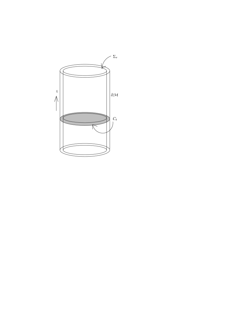
Figure 1: We illustrate in this figure the various slices used in this paper. The shaded area is the initial value surface, $\partial M$ is the conformal boundary of the spacetime and $\Sigma_{r}$ is the regulated surface.

The radial slice $\Sigma_{r}$

The radial slice is defined by its normal $E^{\hat{r}}$. With the coordinate choice in (B.1), this is the $r=const$ slice. The induced metric is given by

$$ds^{2}_{r}=\gamma_{ij}(r,x)\,dx^{i}dx^{j}=\sum_{\hat{i},\hat{j}}\eta_{\hat{i}\hat{j}}\,E^{\hat{i}}\otimes E^{\hat{j}}$$ (B.5)

As $r\to\infty$, $\Sigma_{r}$ approaches the conformal boundary $\partial M$. In this limit the induced metric $\gamma_{ij}(x,r)$ blows up and only a conformal structure is well-defined. One can pick a specific representative $g_{(0)}$ by a specific choice of defining function $\rho$ (a defining function is a positive function that has a single zero at the boundary). Choosing as defining function $\rho=e^{-r}$ we get as a boundary metric

$$ds_{\infty}^{2}=g_{(0)ij}\,dx^{i}dx^{j}=\sum_{\hat{i},\hat{j}}\eta_{\hat{i}\hat{j}}\;e^{\hat{i}}\otimes e^{\hat{j}}$$ (B.6)

where $e^{\hat{i}}=\lim_{r\to\infty}e^{-r}E^{\hat{i}}$.

The time slice $C_{t}$

We consider the time slice $C_{t}$ defined by its normal $E^{\hat{t}}$. The induced metric on $C_{t}$ is

$$ds^{2}_{t} \equiv {}^{t}G_{\mu\nu}dx^{\mu}dx^{\nu}=\left(G_{\mu\nu}+E^{\hat{t}}_{\mu}E^{\hat{t}}_{\nu}\right)dx^{\mu}dx^{\nu}$$ (B.7)

$$= \sum_{\alpha}E^{\hat{\alpha}}\otimes E^{\hat{\alpha}}=E^{\hat{r}}\otimes E^{\hat{r}}+\sum_{a}E^{\hat{a}}\otimes E^{\hat{a}}.$$

The boundary of the time slice $C_{t}\cap\Sigma_{r}$

The induced metric on the intersection of the two slices is

$$ds^{2}_{(rt)}\equiv{}^{t}\gamma_{ij}dx^{i}dx^{j}=\Bigl{(}\,\gamma_{ij}+E^{\hat{t}}_{i}E^{\hat{t}}_{j}\,\Bigr{)}\,dx^{i}dx^{j}=\sum_{a}E^{\hat{a}}\otimes E^{\hat{a}}\\$$

As $r\to\infty$, and with the same defining function as before, we get for the metric on $C_{t}\cap\partial M$

$$ds^{2}_{\infty,t}\equiv{}^{t}g_{(0)ij}dx^{i}dx^{j}=(\,g_{(0)ij}+e^{\hat{t}}_{i}e^{\hat{t}}_{j}\,)dx^{i}dx^{j},$$ (B.8)

where $e^{\hat{j}}_{i}=\lim_{r\to\infty}(e^{-r}\,E^{\hat{j}}_{i})$ is the vielbein of the boundary metric $g_{(0)ij}$.

Appendix C Asymptotic expansions

In this appendix we present some of the technical details needed in order to obtain the asymptotic solution of the Witten spinor.

The dilatation operator (2.7) is given in terms of the vielbein by

$$\delta_{D}=\int d^{d}x\,E^{\hat{j}}_{i}\,\frac{\delta}{\delta E^{\hat{j}}_{i}}\,,$$ (C.9)

and the second fundamental form and radial derivative admits the expansions

$$K^{i}_{\,j}[\gamma] = \delta^{i}_{\,j}+\sum_{k=1}^{[\frac{d-1}{2}]}K_{(2k)}{}^{i}_{j}+K_{(d)}{}^{i}_{j}+\tilde{K}_{(d)}{}^{i}_{j}(-2r)+\cdots$$ (C.10)

$$\partial_{r} = \delta_{D}+\sum_{k=1}^{[\frac{d-1}{2}]}\partial_{r(2k)}+\partial_{r(d)}-(2r)\tilde{\partial}_{r(d)}+\cdots$$

$$\partial_{r(n)} = \int d^{d}xK_{(n)ij}\frac{\delta}{\delta\gamma_{ij}},\qquad\tilde{\partial}_{r(d)}=\int d^{d}x\tilde{K}_{(d)ij}\frac{\delta}{\delta\gamma_{ij}},$$ (C.11)

where $[\frac{d-1}{2}]$ denotes the integer part of $\frac{d-1}{2}$ and $\tilde{K}_{(d)ij}$ is zero when $d$ is odd. Furthermore, since $K_{ij}=\dot{E}_{(i}^{\hat{i}}E_{j)}^{\hat{j}}\eta_{\hat{i}\hat{j}}$, $\dot{E}_{i}^{\hat{i}}$ admits an expansion of the form

$$\partial_{r}E_{i}^{\hat{j}}=E_{i}^{\hat{j}}+\sum_{k=0}^{d-1}\dot{E}_{(k)}{}^{\hat{j}}_{i}+(-2r)\dot{\tilde{E}}_{(d-1)}{}^{\hat{j}}_{i}+\cdots$$ (C.12)

In our coordinate system, the spin connections are given by

$$\Omega_{r}^{\hat{i}\hat{j}}=E^{k[\hat{i}}\partial_{r}E^{\hat{j}]}_{k},\qquad\Omega_{i}^{\hat{j}\hat{r}}=E^{k\hat{j}}K_{ik},\qquad\Omega_{i}^{\hat{i}\hat{j}},$$ (C.13)

and the covariant derivatives take the form,

$$\nabla_{r}\epsilon = (\,\partial_{r}+\frac{1}{4}\,E^{k[\hat{i}}\partial_{r}E^{\hat{j}]}_{k}\,\Gamma_{\hat{i}\hat{j}}+\frac{1}{2}\Gamma_{r}\,)\,\epsilon\,,$$

$$\nabla_{i}\epsilon = (\,D_{i}+\frac{1}{2}E^{k\hat{j}}K_{ik}\Gamma_{\hat{j}\hat{r}}+\frac{1}{2}\Gamma_{i}\,)\,\epsilon\;.$$ (C.14)

where $D_{i}$ is the covariant derivative of the induced metric $\gamma_{ij}$.

Using the results above one can work out the asymptotic expansion of the covariant derivatives and the operator $\hbox to0.0pt{\hbox{$\mskip 1.0mu/$}\hss}\nabla\equiv\Gamma^{\hat{r}}\nabla_{\hat{r}}+\Gamma^{\hat{a}}\nabla_{\hat{a}}$ that appear in the Witten equation,

$$\hbox to0.0pt{\hbox{$\mskip 1.0mu/$}\hss}\nabla_{(0)} = (\delta_{D}\,+\frac{d-1}{2})\Gamma^{\hat{r}}+\frac{d}{2}$$

$$\hbox to0.0pt{\hbox{$\mskip 1.0mu/$}\hss}\nabla_{(1)} = \Gamma^{\hat{a}}D_{\hat{a}}$$ (C.15)

$$\hbox to0.0pt{\hbox{$\mskip 1.0mu/$}\hss}\nabla_{(2n)} = \Bigl{(}2\,\int d^{d}x\,\gamma_{ik}\,K_{(2n)}{}^{i}_{\;\;j}\,\frac{\delta}{\delta\gamma_{jk}}+\frac{1}{4}\,E^{k[\hat{i}}\dot{E}_{(2n-1)}{}^{\hat{j}]}_{k}\,\Gamma_{\hat{i}\hat{j}}+\frac{1}{2}\,K_{(2n)}{}^{\hat{j}}_{\;\hat{a}}\,\Gamma^{\hat{a}}\Gamma_{\hat{j}}\Bigr{)}\,\Gamma^{\hat{r}}$$

$$\hbox to0.0pt{\hbox{$\mskip 1.0mu/$}\hss}\nabla_{(d)} = \Bigl{(}2\,\int d^{d}x\,\gamma_{ik}\,K_{(d)}{}^{i}_{\;\;j}\,\frac{\delta}{\delta\gamma_{jk}}+\frac{1}{4}\,E^{k[\hat{i}}\dot{E}_{(d-1)}{}^{\hat{j}]}_{k}\,\Gamma_{\hat{i}\hat{j}}+\frac{1}{2}\,K_{(d)}{}^{\hat{j}}_{\;\hat{a}}\,\Gamma^{\hat{a}}\Gamma_{\hat{j}}\Bigr{)}\,\Gamma^{\hat{r}}$$

$$\tilde{\hbox to0.0pt{\hbox{$\mskip 1.0mu/$}\hss}\nabla}_{(d)} = \Bigl{(}2\,\int d^{d}x\,\gamma_{ik}\,\tilde{K}_{(d)}{}^{i}_{\;\;j}\,\frac{\delta}{\delta\gamma_{jk}}+\frac{1}{4}\,E^{k[\hat{i}}\dot{\tilde{E}}_{(d-1)}{}^{\hat{j}]}_{k}\,\Gamma_{\hat{i}\hat{j}}+\frac{1}{2}\,\tilde{K}_{(d)}{}^{\hat{j}}_{\;\hat{a}}\,\Gamma^{\hat{a}}\Gamma_{\hat{j}}\Bigr{)}\,\Gamma^{\hat{r}}\;.$$

where $n=1,2,....,[\frac{d-1}{2}]$. Note also that $\delta_{D}E^{k\hat{i}}=-E^{k\hat{i}}$, so $E^{k\hat{i}}\equiv E^{k\hat{i}}_{(1)}$ and that $\tilde{\hbox to0.0pt{\hbox{$\mskip 1.0mu/$}\hss}\nabla}_{(2k+1)}=0$.

Observe that

$$\left[\tilde{\hbox to0.0pt{\hbox{$\mskip 1.0mu/$}\hss}\nabla}_{(d)},P^{\pm}\right]=0,\qquad\left[\hbox to0.0pt{\hbox{$\mskip 1.0mu/$}\hss}\nabla_{(k)},P^{\pm}\right]=0\ (k\neq 1),\qquad\hbox to0.0pt{\hbox{$\mskip 1.0mu/$}\hss}\nabla_{(1)}P^{\pm}=P^{\mp}\hbox to0.0pt{\hbox{$\mskip 1.0mu/$}\hss}\nabla_{(1)}$$

$$\hbox to0.0pt{\hbox{$\mskip 1.0mu/$}\hss}\nabla_{(0)}P^{-}=(-\delta_{D}+\frac{1}{2})P^{-},\qquad\hbox to0.0pt{\hbox{$\mskip 1.0mu/$}\hss}\nabla_{(0)}P^{+}=(\delta_{D}+d-\frac{1}{2})P^{+}$$ (C.16)

We will also use in the main text the asymptotic expansion of the operator $\Gamma^{\hat{a}}\nabla_{\hat{a}}$. It is given by

$$\Gamma^{\hat{a}}\nabla_{\hat{a}(0)} = \frac{d-1}{2}\Gamma^{\hat{r}}+\frac{d-1}{2}=(d-1)P^{+}$$

$$\Gamma^{\hat{a}}\nabla_{\hat{a}(1)} = \Gamma^{\hat{a}}D_{\hat{a}}$$ (C.17)

$$\Gamma^{\hat{a}}\nabla_{\hat{a}(2n)} = \frac{1}{2}\,K^{\hat{j}}_{\;\hat{a}(2n)}\Gamma^{\hat{a}}\Gamma_{\hat{j}}\Gamma^{\hat{r}}\;\;,\;\;n=1,2,....,[\frac{d-1}{2}]$$

$$\Gamma^{\hat{a}}\nabla_{\hat{a}(d)} = \frac{1}{2}\,K^{\hat{j}}_{\;\hat{a}(d)}\Gamma^{\hat{a}}\Gamma_{\hat{j}}\Gamma^{\hat{r}}$$

$$\Gamma^{\hat{a}}\tilde{\nabla}_{\hat{a}(d)} = \frac{1}{2}\,\tilde{K}^{\hat{j}}_{\;\hat{a}(d)}\Gamma^{\hat{a}}\Gamma_{\hat{j}}\Gamma^{\hat{r}}\;.$$

Appendix D Properties under Weyl transformations

We discuss in this appendix the Weyl transformation properties of the conditions of the absence of divergences. We focus on the Weyl transformation properties of (the integral of) $q_{(1)}$ but the discussion can be extend to the other coefficients.

We wish to know how the leading divergence

$$\int_{C_{t}\cap\Sigma_{r}}\sqrt{{}^{t}\gamma}\ q_{(1)}=\int d^{d{-}1}\!x\sqrt{{}^{t}g_{(0)}}\ e^{(d-2)r}\hat{q}_{(1)}(1+{\cal O}(e^{-2r}))$$ (D.18)

$$=-\int d^{d{-}1}\!x\sqrt{{}^{t}g_{(0)}}\ e^{(d-2)r}\hat{\epsilon}_{(-\frac{1}{2})}^{\dagger}\left(\frac{1}{(d-1)}(\Gamma^{\hat{a}}\hat{D}_{\hat{a}})^{2}+\frac{1}{2}\hat{K}_{(2)}{}^{\hat{j}}_{\hat{a}}\Gamma^{\hat{a}}\Gamma_{\hat{j}}\right)\hat{\epsilon}_{(-\frac{1}{2})}\left(1+{\cal O}(e^{-2r})\right)$$

transforms under a local Weyl transformation,

$$\bar{g}_{(0)ij}=e^{2\sigma(x)}g_{(0){ij}}\;.$$ (D.19)

(The hat notation is defined in (2.14)). In order $\bar{g}_{(0)ij}$ to admit a timelike Killing vector we need to impose the following condition on $\sigma(x)$:

$$\sigma_{,\hat{t}}\equiv e^{i}_{\hat{t}}\partial_{i}\sigma=0\;,$$ (D.20)

The Weyl transformation of (D.18) can be worked out using

$$\bar{{\hat{D}}}_{\hat{a}} = e^{-\sigma}\Bigl{(}\,{\hat{D}}_{\hat{a}}+\frac{1}{2}\sigma_{,\hat{b}}\,\Gamma_{\hat{a}}^{\;\;\hat{b}}\Bigr{)}$$ (D.21)

$$\bar{\hat{K}}_{(2)ij} = \hat{K}_{(2)ij}-\hat{D}_{i}\hat{D}_{j}\sigma+\hat{D}_{i}\sigma\hat{D}_{j}\sigma-\frac{1}{2}(\hat{D}\sigma)^{2}g_{(0)ij}$$

$$\bar{\hat{\epsilon}}_{(-\frac{1}{2})} = e^{\sigma/2}\hat{\epsilon}_{(-\frac{1}{2})}.$$

Using these results we derive,

$$\int d^{d{-}1}\!x\sqrt{{}^{t}g_{(0)}}\ e^{(d-2)r}\hat{q}_{(1)}=\int d^{d{-}1}\!x\sqrt{{}^{t}\bar{g}_{(0)}}\ e^{(d-2)(r-\sigma)}\left(\bar{\hat{q}}_{(1)}-\bar{\hat{\epsilon}}_{(-\frac{1}{2})}^{\dagger}\sigma_{,\hat{b}}\Gamma^{\hat{b}\hat{a}}\bar{\hat{D}}_{\hat{a}}\bar{\hat{\epsilon}}_{(-\frac{1}{2})}\right)$$ (D.22)

The overall factor is due to the dilatation transformation property of $q_{(1)}$. We will now show that the additive term is required by the invariance of the Witten-Nester energy under diffeomorphisms.

Weyl transformations on the boundary are induced by special bulk diffeomorphisms,

$$e^{\bar{r}+\sigma(\bar{x})}=e^{r}\,(\,1+{\cal{O}}(e^{-2r})\,),\qquad\ \bar{x}^{i}={x^{i}}\,(\,1+{\cal{O}}(e^{-2r})\,)\;.$$ (D.23)

The regulated Witten-Nester energy is invariant under this transformation provided we also transform the cut-off,

$$E_{NW}[r]=\bar{E}_{NW}[\bar{r}+\sigma(\bar{x})].$$ (D.24)

The normal to the surface $\bar{r}+\sigma(\bar{x})$ is given by $l_{\mu}={\cal D}_{\mu}(\bar{r}+\sigma(\bar{x}))$. Inserting this in the definition of the Witten-Nester energy and considering the leading term in the limit $\bar{r}\to\infty$ we get

$$\bar{E}_{NW}[\bar{r}+\sigma(\bar{x})]\sim\int d^{d{-}1}\!x\sqrt{{}^{t}\bar{g}_{(0)}}\ e^{(d-2)\bar{r}}\left(\bar{\hat{q}}_{(1)}-\bar{\hat{\epsilon}}_{(-\frac{1}{2})}^{\dagger}\sigma_{,\hat{b}}\Gamma^{\hat{b}\hat{a}}\bar{\hat{D}}_{\hat{a}}\bar{\hat{\epsilon}}_{(-\frac{1}{2})}+c.c.\right)$$ (D.25)

which agrees with the rhs of (D.22). The additive term is due to $\sigma$ dependence of the normal vector $l_{\mu}$.

Appendix E Bulk Killing spinors and Witten spinors

We show in this appendix that for an AlAdS spacetime, the bulk Killing spinor $\epsilon$ admits the asymptotic expansion

$$\epsilon=\epsilon_{(-\frac{1}{2})}+\epsilon_{(\frac{1}{2})}+\cdots$$ (E.26)

with

$$\hat{\epsilon}_{(-\frac{1}{2})}=P^{-}\hat{\epsilon}_{(-\frac{1}{2})},\quad\hat{\epsilon}_{(\frac{1}{2})}=-\Gamma^{i}{\hat{D}}_{i}\hat{\epsilon}_{(-\frac{1}{2})}\quad\forall\ i,\ {\rm no\ sum\ over}\ i$$ (E.27)

Furthermore,

$$\xi^{i}=\bar{\hat{\epsilon}}_{(-\frac{1}{2})}\Gamma^{i}\hat{\epsilon}_{(-\frac{1}{2})}$$ (E.28)

is a timelike or null boundary conformal Killing vector.

Proof:
The asymptotic expansion of the covariant derivatives can be obtained from the results in appendix C. Starting from (C.14) we obtain

$$\nabla_{r}\epsilon = \Bigl{(}(\delta_{D}+\frac{1}{2}\Gamma_{\hat{r}})+\nabla_{(2)}+\cdots\Bigr{)}\;\epsilon$$ (E.29)

$$\nabla_{i}\epsilon = (E^{\hat{j}}_{i}\Gamma_{\hat{j}}P^{+}+D_{i}+\nabla_{(2)i}+\cdots)\;\epsilon\;.$$ (E.30)

We can now solve asymptotically the Killing spinor equations

$$\nabla_{\mu}\epsilon=0.$$ (E.31)

The radial equation, $\nabla_{r}\epsilon=0$, implies that

$$\epsilon = e^{\frac{1}{2}r}\hat{\epsilon}_{(-\frac{1}{2})}+e^{-\frac{1}{2}r}\hat{\epsilon}_{(\frac{1}{2})}+\cdots$$ (E.32)

$$\hat{\epsilon}_{(-\frac{1}{2})} = P^{-}\hat{\epsilon}_{(-\frac{1}{2})}\;\;;\;\;\hat{\epsilon}_{(\frac{1}{2})}=P^{+}\hat{\epsilon}_{(\frac{1}{2})}$$ (E.33)

Inserting this in the spatial equations, $\nabla_{i}\epsilon=0$, we obtain

$${\hat{D}}_{i}\hat{\epsilon}_{(-\frac{1}{2})}+\Gamma_{i}\hat{\epsilon}_{(\frac{1}{2})}=0\;,\qquad\Leftrightarrow\qquad\hat{\epsilon}_{(\frac{1}{2})}=-\Gamma^{i}{\hat{D}}_{i}\hat{\epsilon}_{(-\frac{1}{2})}\quad\forall\ i\ ({\rm no\ sum})$$ (E.34)

where ${\hat{D}}_{i}$ and $\Gamma_{i}\equiv e^{\hat{j}}_{i}\Gamma_{\hat{j}}$ are defined with respect to the boundary metric $g_{(0)ij}$.

Notice that an asymptotic Killing spinor is in particular a Witten spinor, but not vice versa. For instance, the sub-leading asymptotic coefficient of a Witten spinor is given by (5.45),

$$\hat{\epsilon}_{(\frac{1}{2})}=-\frac{1}{d-1}\Gamma^{\hat{a}}{\hat{D}}_{\hat{a}}\hat{\epsilon}_{(-\frac{1}{2})}\;,\qquad{\rm Witten\ spinor}$$ (E.35)

Unless $\Gamma^{\hat{a}}\hat{D}_{\hat{a}}\hat{\epsilon}_{(-\frac{1}{2})}=\Gamma^{\hat{b}}\hat{D}_{\hat{b}}\hat{\epsilon}_{(-\frac{1}{2})}$, for all $a$ and $b$, the Witten spinor will not asymptote to a Killing spinor.

The fact that $\xi^{i}=\bar{\hat{\epsilon}}_{(-\frac{1}{2})}\Gamma^{i}\hat{\epsilon}_{(-\frac{1}{2})}$ is a conformal Killing vector follows by direct computation using the asymptotics of the Killing spinor,

$${\hat{D}}_{(i}\,\xi_{j)} = {\hat{D}}_{(i}\,\left(\bar{\hat{\epsilon}}_{(-\frac{1}{2})}\Gamma_{j)}\hat{\epsilon}_{(-\frac{1}{2})}\right)$$ (E.36)

$$= \bar{\hat{\epsilon}}_{(\frac{1}{2})}\Gamma_{(i}\Gamma_{j)}\hat{\epsilon}_{(-\frac{1}{2})}-\bar{\hat{\epsilon}}_{(-\frac{1}{2})}\Gamma_{(j}\Gamma_{i)}\hat{\epsilon}_{(\frac{1}{2})}$$

$$= g_{(0)ij}\,(\,\bar{\hat{\epsilon}}_{(\frac{1}{2})}\hat{\epsilon}_{(-\frac{1}{2})}-\bar{\hat{\epsilon}}_{(-\frac{1}{2})}\hat{\epsilon}_{(\frac{1}{2})}\,)$$

$$= \frac{1}{d}g_{(0)ij}{\hat{D}}_{k}\,(\bar{\hat{\epsilon}}_{(-\frac{1}{2})}\Gamma^{k}\hat{\epsilon}_{(-\frac{1}{2})})$$

$$= \frac{1}{d}g_{(0)ij}\,{\hat{D}}_{k}\xi^{k}.$$

We now prove that $\xi^{\hat{i}}=\bar{\hat{\epsilon}}_{(-\frac{1}{2})}\Gamma^{\hat{i}}\hat{\epsilon}_{(-\frac{1}{2})}$ is timelike or null. Let us introduce the hermitian matrix

$$A=v_{\hat{a}}\Gamma_{\hat{t}}\Gamma^{\hat{a}},\qquad v^{2}\equiv\eta^{\hat{a}\hat{b}}v_{\hat{a}}v_{\hat{b}}=1,\qquad i=\{t,\{a\}\}.$$ (E.37)

and consider $\hat{\epsilon}_{(-\frac{1}{2})}$ that is an eigenvector of $A$,

$$A\hat{\epsilon}_{(-\frac{1}{2})}=a\hat{\epsilon}_{(-\frac{1}{2})}.$$ (E.38)

Since $A^{2}=1,a^{2}=1$ too. Multiplying (E.38) by $\hat{\epsilon}_{(-\frac{1}{2})}^{\dagger}$ and squaring we get

$$(\xi^{\hat{0}})^{2}=\left(\sum_{\hat{a}}v_{\hat{a}}\xi^{\hat{a}}\right)^{2}.$$ (E.39)

Elementary algebra shows that

$$\sum_{\hat{a}<\hat{b}}(\xi^{\hat{a}}v^{\hat{b}}-\xi^{\hat{b}}v^{\hat{a}})^{2}=\sum_{\hat{a}}(\xi^{\hat{a}})^{2}-\left(\sum_{\hat{a}}v_{\hat{a}}\xi^{\hat{a}}\right)^{2}\geq 0,$$ (E.40)

which implies

$$|\xi|^{2}\equiv-(\xi^{\hat{0}})^{2}+\sum_{\hat{a}}(\xi^{\hat{a}})^{2}\leq 0.$$ (E.41)

Appendix F Killing Spinors of AdS_d+1 in global coordinates

We discuss in this appendix the structure of the Killing spinors for AdS_d+1 spacetimes in coordinates

$$ds^{2}=dr^{2}-N_{+}^{2}(r)\,dt^{2}+N_{-}^{2}(r)\,d\Omega_{d-1}^{2}\;,$$ (F.1)

where

$$N_{\pm}(r)=e^{r}\pm\frac{1}{4}e^{-r}$$ (F.2)

and $d\Omega_{d-1}^{2}$ is the standard metric on $S^{d-1}$,

$$d\Omega_{n}^{2}=d\theta_{n}^{2}+\sin^{2}\theta_{n}\,d\Omega_{n-1}^{2}\;\;;\;\;d\Omega_{1}^{2}=d\theta_{1}^{2}\;,$$ (F.3)

The radial coordinate $\rho$ usually used in the standard global coordinates is given by $\rho=N_{-}$.

We find that the Killing spinors can be written in the following compact form

$$\epsilon=e^{\frac{r}{2}}\,\hat{\epsilon}_{(-\frac{1}{2})}+e^{-\frac{r}{2}}\,\hat{\epsilon}_{(\frac{1}{2})}\;,$$ (F.4)

where

$$\hat{\epsilon}_{(-\frac{1}{2})} = P^{-}{\cal{O}}^{+}_{d-1}{\cal{O}}_{d-2}...{\cal{O}}_{1}{\cal{O}}_{t}\eta$$ (F.5)

$$\hat{\epsilon}_{(\frac{1}{2})} = -\frac{1}{2}P^{+}{\cal{O}}^{-}_{d-1}{\cal{O}}_{d-2}...{\cal{O}}_{1}{\cal{O}}_{t}\eta\;,$$

with $\eta$ a constant spinor and

$${\cal{O}}_{t} = e^{-\frac{t}{2}\Gamma^{\hat{t}}}=\cos\frac{t}{2}-\sin\frac{t}{2}\,\Gamma^{\hat{t}}$$ (F.6)

$${\cal{O}}_{j} = e^{\frac{\theta_{j}}{2}\Gamma^{\widehat{j{+}1},\hat{j}}}=\cos\frac{\theta_{j}}{2}+\sin\frac{\theta_{j}}{2}\,\Gamma^{\widehat{j{+}1},\hat{j}}\;\;\;\;\;j=1,..,d-2$$

$${\cal{O}}^{\pm}_{d-1} = \cos\frac{\theta_{d-1}}{2}\pm\sin\frac{\theta_{d-1}}{2}\,\Gamma^{\widehat{d{-}1}}.$$

Proof

The covariant derivatives are given by,

$$\nabla_{\hat{r}} = \partial_{r}+\frac{1}{2}\Gamma_{\hat{r}}$$ (F.7)

$$\nabla_{\hat{t}} = \frac{1}{N_{+}}\,(\,\partial_{t}+e^{r}\Gamma_{\hat{t}}P^{+}+\frac{1}{4}e^{-r}\Gamma_{\hat{t}}P^{-}\,)$$

$$\nabla_{\hat{\theta}_{k}} = \frac{1}{N_{-}}\,(\,\hat{D}_{\hat{k}}+e^{r}\Gamma_{\hat{k}}P^{+}-\frac{1}{4}e^{-r}\Gamma_{\hat{k}}P^{-}\,),\;\;\;\;\;k=1,\ldots,d-1$$

where $\hat{D}_{\hat{k}}=e^{k}_{\hat{k}}\hat{D}_{k}$ denotes the covariant derivatives on the unit sphere. Explicitly,

$$\hat{D}_{k} = \frac{\partial}{\partial\theta_{k}}+\frac{1}{4}\,\omega_{i}^{\;\;kl}\Gamma_{kl}$$ (F.8)

$$\omega_{i}^{\;\;kl} = \delta^{k}_{i}\,\cos\theta_{l}\prod^{l-1}_{m=i+1}\,\sin\theta_{m}\qquad(k<l)\;,$$

$$e^{\hat{k}}_{k} = \prod^{d-1}_{m=k+1}\,\sin\theta_{m}.$$

Using these expressions, one can easily verify that (F.4) satisfy $\nabla_{\hat{r}}\epsilon=\nabla_{\hat{t}}\epsilon=0$, so we concentrate on the spherical part. From (F.7) we see that $\nabla_{\hat{\theta_{k}}}\epsilon=0$ is equivalent to the following equations,

$$\hat{D}_{\hat{k}}\hat{\epsilon}_{(-\frac{1}{2})}+\Gamma_{\hat{k}}\,\hat{\epsilon}_{(\frac{1}{2})} = 0\;,$$ (F.9)

$$\hat{D}_{\hat{k}}\hat{\epsilon}_{(\frac{1}{2})}-\frac{1}{4}\,\Gamma_{\hat{k}}\,\hat{\epsilon}_{(-\frac{1}{2})} = 0\;.$$

These equations are easily shown to hold for $k=d-1$, so in the following we discuss the cases $k=1,2,..,d-2$. Our proof is similar in spirit with the discussion in [42].

We begin with the fact

$$\partial_{j}{\cal{O}}_{k}=\delta_{jk}\,\frac{1}{2}\Gamma^{j+1,j}{\cal{O}}_{j},$$ (F.10)

which can be used to rewrite (F.9) as

$${\cal{O}}^{\pm}_{d-1}\,U_{j}^{\;\;d-2}+\omega_{j}^{\;\;jl}\,\Gamma_{jl}{\cal{O}}^{\pm}_{d-1}-e^{\hat{j}}_{j}\Gamma_{j}{\cal{O}}^{\mp}_{d-1}=0,$$ (F.11)

where $U_{j}^{\;\;k}\;\;(k\leq j)$ is defined by

$$U_{j}^{\;\;k}={\cal{O}}_{k}\,U_{j}^{\;\;k-1}{\cal{O}}^{-1}_{k};\;\;\;\;\;\;U_{j}^{\;\;j}\equiv\Gamma_{j+1,j}\;.$$ (F.12)

Equations (F.11) can further be rewritten as

$${\cal{O}}_{d-1}^{\pm}\,U_{j}^{\;\;d-2}{\cal{O}}_{d-1}^{\mp}+\cos\theta_{d-1}\,\omega_{j}^{\;\;jl}\,\Gamma_{jl}\mp e^{\hat{j}}_{j}\,\Gamma_{j}\,(1\mp\sin\theta_{d-1}\,\Gamma_{d-1})=0\;,$$ (F.13)

where we have used the relations

$${\cal{O}}_{d-1}^{+}\,{\cal{O}}_{d-1}^{-} = {\cal{O}}_{d-1}^{-}\,{\cal{O}}_{d-1}^{+}=\cos\theta_{d-1}$$ (F.14)

$$({\cal{O}}_{d-1}^{\pm})^{2} = 1\pm\sin\theta_{d-1}\,\Gamma_{d-1}\;.$$

Using (F.8) and the relation

$${\cal{O}}^{\pm}_{d-1}\,\Gamma_{j,d-1}\,{\cal{O}}^{\mp}_{d-1}=\Gamma_{j,d-1}\mp\sin\theta_{d-1}\Gamma_{j},$$ (F.15)

one can prove (F.13) provided $U_{j}{}^{k}$ is given by

$$U_{j}^{\;\;k}=-\sum^{k}_{l>j}\omega_{j}^{\;\;jl}\,\Gamma_{jl}-\sec\theta_{k+1}\,\omega_{j}^{\;\;j,k+1}\,\Gamma_{j,k+1}.$$ (F.16)

We now prove this relation by induction. First observe that $U_{j}^{\;\;j}=\Gamma_{j+1,j}$ satisfies (F.16). Suppose now that (F.16) is satisfied for $U_{j}^{\;\;k}$ for some $k<d-2$. Using

$${\cal{O}}_{k+1}\,\Gamma_{j,k+1}{\cal{O}}_{k+1}^{-1}=\cos\theta_{k+1}\,\Gamma_{j,k+1}+\sin\theta_{k+1}\,\Gamma_{j,k+2}\;,$$ (F.17)

one finds that $U_{j}^{\;\;k+1}$ satisfies (F.16) too. This finishes the proof of (F.16) and thus the proof that (F.4) is the Killing spinor of AdS_d+1.

Appendix G Asymptotics of AAdS spacetimes

We obtain in this appendix the coefficients $K_{(2n)ij}[g_{(0)}],n<d$ for AAdS. As mentioned in the main text, it is sufficient to compute them for the exact $AdS$ solution.

Consider $AdS_{d+1}$ with boundary metric $g_{(0)}$ the standard metric on $R\times S^{d-1}$. Then from (2.3) we obtain,

$$g_{(2)ab}=-\frac{1}{2}g_{(0)ab},\qquad g_{(2)tt}=\frac{1}{2}g_{(0)tt},\qquad g_{(4)ij}=\frac{1}{16}g_{(0)ij}.$$ (G.18)

The induced metric and second fundamental form are given by

$$\gamma_{ij} = e^{2r}(g_{(0)ij}+e^{-2r}g_{(2)ij}+e^{-4r}g_{(4)ij})$$

$$K_{ij}[\gamma] = \frac{1}{2}\dot{\gamma}_{ij}=e^{2r}g_{(0)ij}-e^{-2r}g_{(4)ij}\equiv K_{(0)ij}[\gamma]+\cdots+K_{(2n)ij}[\gamma]+\cdots$$ (G.19)

Recall that the coefficient $K_{(2n)ij}$ are local polynomials of dimension $n$ of (covariant derivatives of the) curvature tensor of the induced metric. For the case at hand, this implies that $K_{(2n)ij}$ is proportional to $R^{n}$, where

$$R=(d-1)(d-2)\gamma^{-1},\qquad\gamma=e^{2r}\left(1-\frac{e^{-2r}}{4}\right)^{2}$$ (G.20)

is the curvature scalar of $\gamma_{ij}$. Thus, the expansion in eigenfunctions of the dilation operator is equivalent to an expansion in $\gamma^{-1}$,

$$K_{ab}[\gamma]=\gamma_{ab}\sum_{n=0}\hat{k}_{(2n)}\gamma^{-2n}$$ (G.21)

Inserting this expression in (G.19) yields,

$$\sum_{n=0}\hat{k}_{(2n)}e^{-2nr}\left(1-\frac{e^{-2r}}{4}\right)^{-2n}=(1+\frac{e^{-2r}}{4})(1-\frac{e^{-2r}}{4})^{-1}.$$ (G.22)

Expanding both sides around $r\to\infty$ and matching powers of $e^{-2r}$ determines the coefficients $\hat{k}_{(2n)}$. The first few are given in (8.73).

We next turn to the expansion of the Witten spinor. As mentioned in the main text, we take the Witten spinor to be a Killing spinor up to sufficiently high order, and the Killing spinor is given by

$$\epsilon_{K}(x,r)=e^{\frac{r}{2}}\hat{\epsilon}_{(-\frac{1}{2})}(x)+e^{-\frac{r}{2}}\hat{\epsilon}_{(\frac{1}{2})}(x).$$ (G.23)

To obtain the eigenfunctions of the dilatation operator we should express $\epsilon_{K}(x,r)$ as a series in $\gamma^{-1}$,

$$e_{K}(x,r)=\sum_{m=0}\hat{\epsilon}_{(-\frac{1}{2}+m)}(x)\gamma^{-\frac{1}{2}(-\frac{1}{2}+m)}.$$ (G.24)

Comparing (G.23) and (G.24) determines $\hat{\epsilon}_{(-\frac{1}{2}+m)}(x)$. The first few are given in (8.75).

References

• [1] A. Ashtekar and A. Magnon, “Asymptotically anti-de Sitter space-times”, Class. Quant. Grav. 1 (1984) L39-L44; A. Ashtekar and S. Das, “Asymptotically anti-de Sitter space-times: Conserved quantities,” Class. Quant. Grav.  17 (2000) L17 [arXiv:hep-th/9911230].
• [2] M. Henneaux and C. Teitelboim, “Hamiltonian Treatment Of Asymptotically Anti-De Sitter Spaces,” Phys. Lett. B 142 (1984) 355; “Asymptotically Anti-De Sitter Spaces,” Commun. Math. Phys.  98, 391 (1985).
• [3] C. Fefferman and C. Robin Graham, “Conformal Invariants”, in Elie Cartan et les Mathématiques d’aujourd’hui (Astérisque, 1985) 95.
• [4] J. D. Brown and J. W. . York, “Quasilocal energy and conserved charges derived from the gravitational action,” Phys. Rev. D 47, 1407 (1993).
• [5] M. Henningson and K. Skenderis, “The holographic Weyl anomaly,” JHEP 9807 (1998) 023 [hep-th/9806087]; M. Henningson and K. Skenderis, “Holography and the Weyl anomaly,” Fortsch. Phys.  48 (2000) 125 [hep-th/9812032].
• [6] V. Balasubramanian and P. Kraus, “A stress tensor for anti-de Sitter gravity,” Commun. Math. Phys.  208, 413 (1999) [arXiv:hep-th/9902121].
• [7] P. Kraus, F. Larsen and R. Siebelink, “The gravitational action in asymptotically AdS and flat spacetimes,” Nucl. Phys. B 563 (1999) 259 [hep-th/9906127].
• [8] S. de Haro, S. N. Solodukhin and K. Skenderis, “Holographic reconstruction of spacetime and renormalization in the AdS/CFT correspondence,” Commun. Math. Phys.  217 (2001) 595 [hep-th/0002230].
• [9] K. Skenderis, “Asymptotically anti-de Sitter spacetimes and their stress energy tensor,” Int. J. Mod. Phys. A 16, 740 (2001) [arXiv:hep-th/0010138].
• [10] M. Bianchi, D. Z. Freedman and K. Skenderis, “How to go with an RG flow,” JHEP 0108 (2001) 041 [arXiv:hep-th/0105276].
• [11] M. Bianchi, D. Z. Freedman and K. Skenderis, “Holographic renormalization,” Nucl. Phys. B 631 (2002) 159 [arXiv:hep-th/0112119].
• [12] D. Martelli and W. Muck, “Holographic renormalization and Ward identities with the Hamilton-Jacobi method,” Nucl. Phys. B 654 (2003) 248 [arXiv:hep-th/0205061];
• [13] K. Skenderis, “Lecture notes on holographic renormalization,” Class. Quant. Grav.  19 (2002) 5849 [hep-th/0209067].
• [14] I. Papadimitriou and K. Skenderis, “AdS/CFT correspondence and geometry,” arXiv:hep-th/0404176.
• [15] I. Papadimitriou and K. Skenderis, “Correlation functions in holographic RG flows,” JHEP 0410 (2004) 075 [arXiv:hep-th/0407071].
• [16] I. Papadimitriou and K. Skenderis, “Thermodynamics of Asymptotically locally AdS spacetimes,” JHEP 08 (2005) 004 hep-th/0505190.
• [17] L. F. Abbott and S. Deser, “Stability Of Gravity With A Cosmological Constant,” Nucl. Phys. B 195 (1982) 76.
• [18] S. W. Hawking and G. T. Horowitz, “The Gravitational Hamiltonian, action, entropy and surface terms,” Class. Quant. Grav.  13 (1996) 1487 [arXiv:gr-qc/9501014].
• [19] S. Hollands, A. Ishibashi and D. Marolf, “Comparison between various notions of conserved charges in asymptotically AdS-spacetimes,” arXiv:hep-th/0503045.
• [20] R. M. Wald and A. Zoupas, “A General Definition of ”Conserved Quantities” in General Relativity and Other Theories of Gravity,” Phys. Rev. D 61, 084027 (2000) [arXiv:gr-qc/9911095] and references therein.
• [21] G. W. Gibbons, C. M. Hull and N. P. Warner, “The Stability Of Gauged Supergravity,” Nucl. Phys. B 218 (1983) 173.
• [22] E. Witten, “A Simple Proof Of The Positive Energy Theorem,” Commun. Math. Phys.  80, 381 (1981).
• [23] E. Witten, “Instability Of The Kaluza-Klein Vacuum,” Nucl. Phys. B 195, 481 (1982).
• [24] C. LeBrun, “Counter-Examples to the Generaized Positive Action Conjecture”, Commun. Math. Phys. 118 (1988) 591-596.
• [25] G. T. Horowitz and R. C. Myers, “The AdS/CFT correspondence and a new positive energy conjecture for general relativity,” Phys. Rev. D 59, 026005 (1999) [arXiv:hep-th/9808079].
• [26] C.R. Graham, “Volume and Area Renormalizations for Conformally Compact Einstein Metrics”, math.DG/9909042.
• [27] M. T. Anderson, “Geometric aspects of the AdS/CFT correspondence,” arXiv:hep-th/0403087.
• [28] K. Skenderis and S. N. Solodukhin, “Quantum effective action from the AdS/CFT correspondence,” Phys. Lett. B 472 (2000) 316 [arXiv:hep-th/9910023].
• [29] A. Petkou and K. Skenderis, “A non-renormalization theorem for conformal anomalies,” Nucl. Phys. B 561 (1999) 100 [arXiv:hep-th/9906030].
• [30] J. Nester, “A new gravitational expression with a simple positivity proof”, Phys. Lett. 83A, 241 (1981).
• [31] D. Z. Freedman, C. Nunez, M. Schnabl and K. Skenderis, “Fake supergravity and domain wall stability,” Phys. Rev. D 69, 104027 (2004) [arXiv:hep-th/0312055].
• [32] G. W. Gibbons, S. W. Hawking, G. T. Horowitz and M. J. Perry, “Positive Mass Theorems For Black Holes,” Commun. Math. Phys.  88, 295 (1983).
• [33] S. Davis, “Definition Of Conserved Quantities In Asymptotically Anti-De Sitter Space-Times,” Phys. Lett. B 166 (1986) 127.
• [34] A. Cappelli and A. Coste, “On The Stress Tensor Of Conformal Field Theories In Higher Dimensions,” Nucl. Phys. B 314, 707 (1989).
• [35] J. M. Izquierdo and P. K. Townsend, “Supersymmetric space-times in (2+1) adS supergravity models,” Class. Quant. Grav.  12 (1995) 895 [arXiv:gr-qc/9501018].
• [36] M. Banados, C. Teitelboim and J. Zanelli, “The Black hole in three-dimensional space-time,” Phys. Rev. Lett.  69, 1849 (1992) [arXiv:hep-th/9204099]; M. Banados, M. Henneaux, C. Teitelboim and J. Zanelli, “Geometry of the (2+1) black hole,” Phys. Rev. D 48, 1506 (1993) [arXiv:gr-qc/9302012].
• [37] O. Coussaert and M. Henneaux, “Supersymmetry of the (2+1) black holes,” Phys. Rev. Lett.  72, 183 (1994) [arXiv:hep-th/9310194].
• [38] N. R. Constable and R. C. Myers, “Spin-two glueballs, positive energy theorems and the AdS/CFT correspondence,” JHEP 9910, 037 (1999) [arXiv:hep-th/9908175].
• [39] G. J. Galloway, S. Surya and E. Woolgar, “A uniqueness theorem for the adS soliton,” Phys. Rev. Lett.  88, 101102 (2002) [arXiv:hep-th/0108170]; “On the geometry and mass of static, asymptotically AdS spacetimes, and the uniqueness of the AdS soliton,” Commun. Math. Phys.  241, 1 (2003) [arXiv:hep-th/0204081].
• [40] P. K. Townsend, “Positive Energy And The Scalar Potential In Higher Dimensional (Super)Gravity Theories,” Phys. Lett. B 148, 55 (1984).
• [41] K. Skenderis and P. K. Townsend, “Gravitational stability and renormalization-group flow,” Phys. Lett. B 468, 46 (1999) [arXiv:hep-th/9909070].
• [42] H. Lu, C. N. Pope and J. Rahmfeld, ”A construction of Killing spinors on $S^{n}$,” J. Math. Phys.  40 (1999) 4518 [arXiv:hep-th/9805151].