Membrane Instantons and de Sitter Vacua

Abstract:

We investigate membrane instanton effects in type IIA strings compactified on rigid Calabi-Yau manifolds. These effects contribute to the low-energy effective action of the universal hypermultiplet. In the absence of additional fivebrane instantons, the quaternionic geometry of this hypermultiplet is determined by solutions of the three-dimensional Toda equation. We construct solutions describing membrane instantons, and find perfect agreement with the string theory prediction. In the context of flux compactifications we discuss how membrane instantons contribute to the scalar potential and the stabilization of moduli. Finally, we demonstrate the existence of meta-stable de Sitter vacua.

1 Introduction

A central question in string theory is the existence and viability of “semi-realistic” four-dimensional ground states. In this context studying the vacuum structure arising from flux compactifications has recently attracted considerable attention. In particular, [1] (KKLT) provided a qualitative picture for obtaining meta-stable de Sitter (dS) vacua from compactifications of the type IIB string, in which fluxes and non-perturbative instanton effects play a crucial role. In this paper we consider membrane instanton corrections arising in the compactification of the type IIA string on rigid Calabi-Yau threefolds (CY₃) and show that including background fluxes and these non-perturbative corrections can provide another scenario to stabilize all hypermultiplet moduli at a meta-stable de Sitter vacuum.

The four-dimensional low-energy effective actions for string compactifications preserving some supersymmetry are supergravity actions coupled to matter multiplets. When fluxes are turned on, one typically obtains gauged supergravities with a potential for the scalar fields of the matter multiplets. The properties and extrema of such potentials are of great importance for string cosmology, since they determine the vacuum structure of the theory. In recent years, string theorists have searched intensively for models in which the potential admits vacua with a (small) positive cosmological constant. It turned out that it is fairly difficult to realize such vacua in string theory, as they can only be meta-stable (see e.g. [2] for a review).

A qualitative picture on how such vacua can be obtained was given in [1] in the context of type IIB flux compactifications on orientifolds. In this case the four-dimensional effective action has $N=1$ supersymmetry, and the potential is determined by a holomorphic superpotential. The KKLT scenario relies on three contributions to the superpotential: first there is a classical contribution coming from fluxes which stabilizes all moduli except the volume modulus which does not enter into a scalar potential of no-scale type. This modulus is then stabilized by a non-perturbative contribution to the potential due to D-instantons or gaugino condensation. These two ingredients stabilize all moduli in a supersymmetric AdS vacuum. In the third step a (small) positive energy contribution, as e.g. an anti-D3-brane, is added which lifts the AdS vacuum to a positive cosmological constant. Since its first proposal, possible realizations of this scenario either within type IIB orientifold compactifications or their F-theory descriptions have been studied intensively [3, 4, 5].

One of the goals of this paper is to provide an alternative scenario in the context of type IIA string theory compactified on a CY₃. Without including background fluxes the LEEA arising from these compactifications is a four-dimensional $N=2$ supergravity action coupled to $h_{1,1}$ vector and $h_{1,2}+1$ hypermultiplets. There is no scalar potential and the scalars (moduli) of the theory parameterize flat directions. The coupling to $N=2$ supergravity requires the scalars of the hypermultiplets to parameterize a quaternion-Kähler manifold [6]. The dilaton that controls the quantum corrections sits in a hypermultiplet (the universal hypermultiplet), and hence it is the quaternionic geometry that receives quantum corrections. Besides perturbative corrections, there are also non-perturbative instanton effects obtained by wrapping Euclidean D-branes around supersymmetric cycles of the internal manifold [7, 8]. From the counting of fermionic zero modes one can derive that they contribute to the low-energy effective action. In the KKLT models they contribute to the superpotential for the $N=1$ chiral multiplets, whereas in our case they correct the hypermultiplet scalar metric.

In this paper, we focus on the special case of the universal hypermultiplet, which can be obtained by compactifying on a rigid CY₃, having $h_{1,2}=0$. We restrict ourselves to rigid CY manifolds, because we will be able to explicitly determine the instanton corrections in this special case only. The general situation when more complex structure moduli are present is technically more difficult because of the complicated nature of the quaternion-Kähler geometry. We believe, however, that our main conclusion will still persist in this case.

The classical quaternionic geometry of the universal hypermultiplet is well-known [9], and recently the perturbative corrections were found in [10], see also [11]. Non-perturbatively, there are both membrane and NS fivebrane instanton corrections [7], but in this paper we shall consider membrane instantons only. In this case the constraints from quaternionic geometry are captured by solutions of the three-dimensional Toda equation. This fact was, to our knowledge, first observed in [22] (see also [23, 24]). One of the main results of this paper is that we construct new solutions of the Toda equation that correspond to membrane instanton expansions. We have not uniquely fixed the solution, and at each order in the instanton expansion, there is still an undetermined integration coefficient that can in principle be computed in string theory. The solution of the Toda equation then determines the quaternion-Kähler (QK) metric in the ungauged supergravity effective action. As we will show, our results are in complete agreement with the predictions made in [7].

Including background fluxes in the compactification leads to four-dimensional $N=2$ gauged supergravity [25, 26, 27] where some isometries of the hypermultiplet scalar manifold are gauged [28, 29]. This gauging induces a scalar potential in the LEEA which depends on the geometrical quantities of the QK space, such as the moment maps and the metric. It is therefore clear that the potential will receive quantum corrections, determined e.g. by the QK metric. We must be careful with this procedure, since isometries of the classical hypermultiplet moduli space can be broken by quantum corrections. This is already the case perturbatively [10, 11]. Non-perturbatively, isometries can get broken to discrete subgroups. To gauge an isometry in supergravity, the standard methods require an unbroken and continuous isometry. However, in the absence of fivebrane instantons, we explain how to find such an isometry, and moreover we show how the corresponding potential can be obtained from a flux compactification of the type discussed in [28].

In both the KKLT models with $N=1$, and as we will see, in our models with $N=2$, it is crucial to take into account the quantum corrections to the low-energy effective action. In particular, including the instanton corrections to the potential is an essential step for stabilizing the dilaton and finding meta-stable de Sitter vacua. This was the case in KKLT, and also applies to our models. In our set-up, we only study the hypermultiplet moduli in detail, and comment on the Kähler moduli at the end of the paper. In that case, the potential only depends on the hypermultiplet scalars and is determined by the solution of the Toda equation. As our solution still contains undetermined integration constants (which, in principle, should be determined by string theory), it is therefore perhaps not too surprising that one can choose coefficients that give de Sitter vacua. In a way, choosing these coefficients mimics stabilizing the volume modulus in the KKLT set-up.

The remainder of the paper is organized as follows. In section 2 we begin by describing the supergravity set-up for our investigations. The moduli space metric of the universal hypermultiplet is introduced and its possible quantum corrections are discussed qualitatively. We then show in section 3 how this metric fits into a general framework for four-dimensional QK geometries with one isometry, which are governed by the three-dimensional Toda equation. In section 4 we derive the leading terms of a solution to this equation describing non-perturbative quantum effects due to membrane instantons. Section 5 is devoted to a comparison of our results with string theory predictions on how these instanton corrections contribute to the four-fermion coupling; we shall find perfect agreement. Finally, in section 6 we investigate the effects of these corrections on the scalar potential that arises by gauging the one remaining isometry of the moduli space metric. It turns out that the undetermined parameters can be such that the potential develops a local meta-stable de Sitter minimum. After the conclusions we provide technical details in several appendices.

2 Supergravity description

For type IIA string theories compactified on a CY₃ manifold, the low-energy effective action is that of four-dimensional $N=2$ supergravity coupled to $h_{1,1}$ vector multiplets, $h_{1,2}$ hypermultiplets, and one tensor multiplet that contains the dilaton [32]. In the case of a rigid CY₃, there are no complex structure moduli: $h_{1,2}=0$. Suppressing the vector multiplets, the resulting four-dimensional low-energy effective action is that of a tensor multiplet coupled to $N=2$ supergravity, and the bosonic part of the Lagrangian at string tree-level is given by

$$e^{-1}\mathcal{L}_{\mathrm{T}} =-R-\frac{1}{2}\,\partial^{\mu}\phi\,\partial_{\mu}\phi+\frac{1}{2}\,\mathrm{e}^{2\phi}H^{\mu}H_{\mu}$$

$$\quad\,-\frac{1}{4}\,F^{\mu\nu}F_{\mu\nu}-\frac{1}{2}\,\mathrm{e}^{-\phi}\big{(}\partial^{\mu}\chi\,\partial_{\mu}\chi+\partial^{\mu}\varphi\,\partial_{\mu}\varphi\big{)}-\frac{1}{2}\,H^{\mu}\big{(}\chi\partial_{\mu}\varphi-\varphi\partial_{\mu}\chi\big{)}\ ,$$ (1)

where $H^{\mu}=\tfrac{1}{6}\,\varepsilon^{\mu\nu\rho\sigma}H_{\nu\rho\sigma}$ is the dual NS 2-form field strength. The first line comes from the NS sector in ten dimensions, and $\phi$ together with $H^{\mu}$ forms an $N=1$ tensor multiplet. The second line descends from the RR sector. In particular, the graviphoton with field strength $F_{\mu\nu}$ descends from the ten-dimensional RR 1-form, and $\varphi$ and $\chi$ can be combined into a complex scalar $C$ that descends from the holomorphic components of the RR 3-form with (complex) indices along the holomorphic 3-form of the CY₃. Notice the presence of constant shift symmetries on both $\chi$ and $\varphi$. Together with a rotation on $\chi$ and $\varphi$ they form a three-dimensional subgroup of symmetries.

The tensor multiplet Lagrangian (2) is dual to the universal hypermultiplet. This can be seen by dualizing the 2-form into an axionic pseudoscalar field $\sigma$, after which one obtains (modulo a surface term)

$$e^{-1}\mathcal{L}_{\mathrm{UH}} =-R-\frac{1}{4}\,F^{\mu\nu}F_{\mu\nu}-\frac{1}{2}\,\partial^{\mu}\phi\,\partial_{\mu}\phi-\frac{1}{2}\,\mathrm{e}^{-\phi}\big{(}\partial^{\mu}\chi\,\partial_{\mu}\chi+\partial^{\mu}\varphi\,\partial_{\mu}\varphi\big{)}$$

$$\quad\,-\frac{1}{2}\,\mathrm{e}^{-2\phi}\big{(}\partial_{\mu}\sigma+\chi\partial_{\mu}\varphi\big{)}^{2}\ .$$ (2)

The four scalars define the classical universal hypermultiplet at string tree-level, a non-linear sigma model with a quaternion-Kähler target space $\mathrm{SU}(1,2)/\mathrm{U}(2)$ [9]. The metric can be written as

$$\mathrm{d}s^{2}=G_{AB}\,\mathrm{d}\phi^{A}\,\mathrm{d}\phi^{B}=\mathrm{d}\phi^{2}+\mathrm{e}^{-\phi}(\mathrm{d}\chi^{2}+\mathrm{d}\varphi^{2})+\mathrm{e}^{-2\phi}(\mathrm{d}\sigma+\chi\mathrm{d}\varphi)^{2}\ .$$ (3)

This manifold has an $\mathrm{SU}(1,2)$ group of isometries, with a three-dimensional Heisenberg subalgebra that generates the following shifts on the fields,

$$\phi\rightarrow\phi\ ,\qquad\chi\rightarrow\chi+\gamma\ ,\qquad\varphi\rightarrow\varphi+\beta\ ,\qquad\sigma\rightarrow\sigma-\alpha-\gamma\,\varphi\ ,$$ (4)

where $\alpha$, $\beta$, $\gamma$ are real (finite) parameters.

Quantum corrections, both perturbative and non-perturbative, will break some of the isometries and alter the classical moduli space of the universal hypermultiplet, while keeping the quaternion-Kähler property intact, as required by supersymmetry [6]. At the perturbative level, a non-trivial one-loop correction modifies the low-energy tensor multiplet Lagrangian (2), as was shown in [10]. After dualization, this corrects the universal hypermultiplet metric (3), while still preserving the isometries (4). More recently, this one-loop correction was written and analyzed in the language of projective superspace in [11], using the tools developed in [33].

At the non-perturbative level, there can be membrane and fivebrane instantons. The latter were analyzed in [12]. Membrane instantons, which we are focussing on in this paper, arise from wrapping Euclidean D2-branes around three-cycles in the CY₃ [7]. For rigid Calabi-Yau’s, there are two kind of membrane instantons, as there are two (supersymmetric) three-cycles that the membrane can wrap around. Correspondingly, there will be two membrane instanton charges. These instantons also have an effective supergravity description, as was shown in [17, 18]. The two instanton charges correspond to the shift symmetries in $\chi$ and $\varphi$, as written down in (4). We denote these charges by $Q_{\chi}$ and $Q_{\varphi}$ respectively. They can also be understood as being the charges of the corresponding dual 3-form field strengths that appear after dualizing one of the scalars $\chi$ or $\varphi$ to a 2-form. Upon doing so, the tensor multiplet becomes a double-tensor multiplet, in which the instanton solution can be derived from a Bogomol’nyi equation [17, 18]. Following this procedure, it becomes clear that only one charge can be switched on simultaneously, either $Q_{\chi}$ or $Q_{\varphi}$, depending on which scalar was dualized to a tensor. One cannot dualize both scalars to tensors, as the two shift symmetries on $\chi$ and $\varphi$ do not commute. In section 5, we will rederive this property from a string theory perspective.

The instanton action is inversely proportional to the string coupling, which, in our conventions, is defined as

$$g_{s}=\mathrm{e}^{-\phi_{\infty}/2}\ .$$ (5)

The membrane instanton action, say for the $\varphi$-instanton, then is [17, 18]

$$S_{\mathrm{inst}}=2\,\frac{|Q_{\varphi}|}{g_{s}}+\mathrm{i}\varphi\,Q_{\varphi}\ .$$ (6)

The imaginary term comes from a surface term that arises upon dualizing the tensor to a scalar. It involves the zero mode of the dual scalar $\varphi$, which can be identified with the value of the field at infinity. Its presence breaks the shift symmetry in $\varphi$ to a discrete subgroup. A similar formula also holds for the $\chi$-instanton, by simply replacing $\varphi$ by $\chi$. Notice also the factor $2$ in front of the real part of the instanton action (6). This will become important later.

To compare, the NS-fivebrane instanton action is inversely proportional to the square of the string coupling and, in the same normalization as above, has no factor of 2 in front [12]. It has a theta-angle-like term proportional to the zero mode of $\sigma$. As long as we don’t switch on fivebrane instantons, the continuous shift symmetry in $\sigma$ will remain an exact symmetry. In other words, in the absence of fivebrane instantons, the quantum corrected universal hypermultiplet moduli space will be a quaternionic manifold with a (non-compact) U(1) isometry. Such manifolds have been classified by mathematicians in terms of a single function, as we describe in the next section.

3 Toda equation and universal hypermultiplet

As explained in the previous section, the effect of membrane instantons is to modify the hypermultiplet moduli space non-perturbatively, in a way consistent with the constraints from quaternion-Kähler (QK) geometry. In the absence of fivebranes the quaternionic manifold has an isometry that acts as a shift in the NS scalar $\sigma$. In this section, we discuss the geometry of QK manifolds with a U(1) isometry, and explain how the universal hypermultiplet fits into this framework.

3.1 The Przanowski-Tod metric

In [34] Przanowski derived the general form of four-dimensional quaternion-Kähler metrics with (at least) one Killing vector. It was later rederived by Tod [35]. The Przanowski-Tod (PT) metric in local coordinates $(r,u,v,t)$ reads

$$\mathrm{d}s^{2}=\frac{1}{r^{2}}\Big{[}f\mathrm{d}r^{2}+f\mathrm{e}^{h}(\mathrm{d}u^{2}+\mathrm{d}v^{2})+f^{-1}(\mathrm{d}t+\Theta)^{2}\Big{]}\ .$$ (7)

The isometry acts as a shift in the coordinate $t$. The metric is determined in terms of one scalar function $h(r,u,v)$, which is subject to the three-dimensional Toda equation

$$(\partial_{u}^{2}+\partial_{v}^{2})h+\partial_{r}^{2}\,\mathrm{e}^{h}=0\ .$$ (8)

The function $f(r,u,v)$ is not independent, but related to $h$ through

$$f=-\frac{3}{2\Lambda}\big{(}2-r\partial_{r}h\big{)}\ ,$$ (9)

while the 1-form $\Theta(r,u,v)=\Theta_{r}\mathrm{d}r+\Theta_{u}\mathrm{d}u+\Theta_{v}\mathrm{d}v$ is a solution to the equation

$$\mathrm{d}\Theta=(\partial_{u}f\,\mathrm{d}v-\partial_{v}f\,\mathrm{d}u)\wedge\mathrm{d}r+\partial_{r}(f\mathrm{e}^{h})\,\mathrm{d}u\wedge\mathrm{d}v\ .$$ (10)

Manifolds with such a metric are Einstein with anti-selfdual Weyl tensor, and $\Lambda$ in (9) is the target space cosmological constant, $R_{AB}=\Lambda G_{AB}$.

As long as at least one isometry remains unbroken, the universal hypermultiplet moduli space metric (3) is of this form. Its Ricci tensor is found to be $R_{AB}=(-3/2)G_{AB}$, thus $\Lambda=-3/2$ in our conventions.

It is quite remarkable that the non-perturbative structure of the universal hypermultiplet is fully encoded by the solutions of the Toda equation. This equation has been studied by mathematicians in the context of three-dimensional Einstein-Weyl spaces and hyperkähler manifolds [36, 37, 38] (see also appendix B). More recently, a large class of solutions of the Toda equation was constructed by [39], see also [40]. Unfortunately these do not seem to satisfy the boundary conditions required by our set-up, so in the next section we will construct new solutions that describe membrane instanton effects.

Integrable structures, including the Toda hierarchy, have also been discovered in topological string theory [41]. Related to this, the Toda equation also appears in the non-perturbative description of the non-critical $c=1$ string theory [42]. It would be interesting to better understand the connection, if any, to our work. Finally, we mention that the Toda equation also plays an important role in classifying BPS vacua in M-theory [43].

3.2 Symmetries, moment maps, and 4-fermion couplings

Clearly, the PT metric has a Killing vector $\partial_{t}$ corresponding to a shift symmetry in $t$. In coordinates $(r,u,v,t)$, this Killing vector is given by

$$k^{A}=(\,0\,,\,0\,,\,0\,,\,e_{0}\,)^{\mathrm{T}}\ ,\qquad e_{0}\in\fieldR\ .$$ (11)

The moment maps of the shift symmetry can be computed from (78), which we do in appendix A.2. The result is independent of the functions $f$, $h$ and $\Theta$, and reads

$$P^{1}=0\ ,\qquad P^{2}=0\ ,\qquad P^{3}=\frac{e_{0}}{r}\ .$$ (12)

Furthermore, $4n$-dimensional quaternion-Kähler manifolds admit a completely symmetric rank four tensor $\mathcal{W}_{\alpha\beta\gamma\delta}$, where $\alpha=1,...,2n$ labels the $\mathrm{USp}(2n)$ index that is part of the holonomy group of QK manifolds. This tensor can be constructed out of the Riemann curvature tensor; its definition and properties are discussed in [45], which we summarize in appendix A.3. In $N=2$ supergravity effective actions, the $\mathcal{W}$-tensor is contracted with four hyperinos; it will play an important role in section 5. In our case, the QK manifold is four-dimensional and hence $n=1$.

For the PT metric we carry out its construction in appendix A.3 and state here only the final result:

$$\mathcal{W}_{1111} =4r^{2}f^{-3}\mathrm{e}^{-h}\big{[}f(\partial^{2}_{\bar{z}}f-\partial_{\bar{z}}h\,\partial_{\bar{z}}f)-3(\partial_{\bar{z}}f)^{2}\big{]}$$

$$\mathcal{W}_{2111} =r^{2}f^{-3}\mathrm{e}^{-h/2}\big{[}2f\,\partial_{r}\partial_{\bar{z}}f-3(f\,\partial_{r}h+2\partial_{r}f)\,\partial_{\bar{z}}f+f^{2}\partial_{r}\partial_{\bar{z}}h\big{]}$$

$$\mathcal{W}_{2211} =-r^{2}f^{-3}\big{[}f\big{(}r\partial^{3}_{r}h-(\partial_{r}h)^{2}\big{)}-4\mathrm{e}^{-h}\,\partial_{z}f\,\partial_{\bar{z}}f+2(\partial_{r}f)^{2}\big{]}$$

$$\mathcal{W}_{2221} =-r^{2}f^{-3}\mathrm{e}^{-h/2}\big{[}2f\,\partial_{r}\partial_{z}f-3(f\,\partial_{r}h+2\partial_{r}f)\,\partial_{z}f+f^{2}\partial_{r}\partial_{z}h\big{]}$$

$$\mathcal{W}_{2222} =4r^{2}f^{-3}\mathrm{e}^{-h}\big{[}f(\partial^{2}_{z}f-\partial_{z}h\,\partial_{z}f)-3(\partial_{z}f)^{2}\big{]}\ .$$ (13)

Here we have introduced the complex variable $z=u+\mathrm{i}v$ in order to write the components of $\mathcal{W}_{\alpha\beta\gamma\delta}$ in a compact way. We will use this tensor in a comparison of the properties of our instanton corrected universal hypermultiplet metric with the results for four-fermi correlation functions computed in string theory [7].

3.3 The universal hypermultiplet in the PT framework

To rewrite the metric (3) in the PT form, we have to identify the moduli of the universal hypermultiplet with the PT coordinates. This must be done consistently with the isometries, in particular with the shift symmetry in the coordinate $t$. From the Heisenberg algebra of isometries (4) it is apparent that one can choose to identify $t$ with either $\sigma$ or $\varphi$. The shift symmetries are generated by the parameters $\alpha$ and $\beta$, respectively. This leads to two ‘dual’ representations of the PT metric that describe the same moduli space. We can call these bases the membrane and the fivebrane basis, respectively.

In the membrane basis, which is the relevant basis for our purposes, we identify the coordinate $t$ with $\sigma$, such that the $\alpha$-shift symmetry is manifest. This is because of the absence of fivebrane instantons, which would break the continuous $\alpha$-shift symmetry to a discrete subgroup [12]. So, the coordinates can be chosen as

$$t=\sigma\ ,\qquad r=\mathrm{e}^{\phi}\ ,\qquad u=\chi\ ,\qquad v=\varphi\ .$$ (14)

In this basis, the classical moduli space metric of the universal hypermultiplet corresponds to the solution $\mathrm{e}^{h}=r$ of the Toda equation (8). It follows that $f=1$ and $\Theta=u\,\mathrm{d}v$, the latter being defined only modulo an exact form.

As mentioned above, besides the instanton contributions that we want to determine in this paper, there are also perturbative quantum corrections to the moduli space metric [10]. These can easily be incorporated in our approach: Observe that with $h(r,u,v)$ also $h(r+c,u,v)$ is a solution to the Toda equation for constant $c\in\fieldR$. Applied to the classical solution $\mathrm{e}^{h}=r$, we obtain

$$\mathrm{e}^{h}=r+c\ ,\qquad f=\frac{r+2c}{r+c}\ ,\qquad\Theta=u\,\mathrm{d}v\ ,$$ (15)

which turns out to describe the 1-loop (in the string frame) corrected metric of [10] if we identify

$$c=-\frac{4\,\zeta(2)\,\chi(X)}{(2\pi)^{3}}=-\frac{1}{6\pi}\,(h_{1,1}-h_{1,2})\ .$$ (16)

Here $h_{1,1}$ and $h_{1,2}$ are the Hodge numbers of the CY threefold $X$ on which the type IIA string has been compactified; for rigid CY’s, where $h_{1,2}=0$, we have the important bound $c<0$. The function $h$ in (15) is simply the general $(u,v)$-independent solution to the Toda equation (modulo a constant rescaling of $r$); in this sense the perturbative corrections appear naturally. The PT coordinate $r$ is related to $\rho$ in [10] through $r=\rho^{2}-c=\mathrm{e}^{\phi}$; the relation between the fields and PT coordinates receives no (perturbative) quantum corrections.

Note that if we consider $c<0$, the function $f$ in (15) becomes negative for $r<2|c|$, which results in a negative-definite metric (7). We thus have to restrict $r$ to the open interval $2|c|<r<\infty$.

4 Instanton corrections

In this section, we construct solutions to the Toda equation (8) that include an (infinite) series of exponential corrections describing the membrane instantons. As we have learned from the supergravity description, the real part of the instanton action is inversely proportional to the dilaton, which becomes the square root of the radial variable $r$. The precise form of the supergravity instanton action is given in (6). This motivates us to make a general ansatz of the form

$$\mathrm{e}^{h}=r+\sum_{n\geq 1}\,\sum_{m}\,f_{n,m}(u,v)\,r^{-m/2+\alpha}\,\mathrm{e}^{-2n\sqrt{r}}\ .$$ (17)

As explained in the previous section, one can shift the value of $r$ with a constant to construct a new solution. This will then include the perturbative one-loop correction of [10]. The power series in $r$ in front of the exponent describes the perturbative corrections around the instantons. Using (5) we have that $r^{-m/2}=g_{s}^{m}$, and the sum over $m$ is over the integers . At each instanton level $n$, there is a lowest value $m_{n}$ that defines the leading term in the expansion,

$$f_{n,m}(u,v)=0\quad\text{for}\quad m<m_{n}\ .$$ (18)

We have also introduced a parameter $\alpha$ which, without loss of generality, lies in the interval $[0,1/2[$. This leaves open the possibility that the leading term is not an integer power of $g_{s}$, as e.g. in [14]. We will show later on that the Toda equation enforces $\alpha=0$. With the $r$-dependence made explicit, solving the Toda equation amounts to solving the differential equations for the functions $f_{n,m}(u,v)$. These are of the type of inhomogeneous Laplace equations, and we can solve them iteratively, order by order in $n$ and $m$, to any order needed.

To get some additional insight, we focus for a moment on the asymptotic (large $r$) behavior of the solution. We can then further specify the ansatz as

$$\mathrm{e}^{h}=r+A\cos(k_{u}u+k_{v}v)\,r^{\beta}\mathrm{e}^{-2k\sqrt{r}}\ ,$$ (19)

with $A$ a normalization constant. One can now check that, to leading order, the Toda equation is satisfied for any value of $\beta$, provided that

$$k^{2}=k_{u}^{2}+k_{v}^{2}\ .$$ (20)

This asymptotic behavior indeed reproduces leading order charge $k$ instanton effects, including a one-loop correction in front of the exponent. The cosine in the ansatz (19) could also be replaced by a sine, or a linear combination. Rewriting them in terms of exponentials, one produces theta-angle like terms for both instantons and anti-instantons, depending on the signs of $(k_{u},k_{v})$. The relation (20) is completely consistent with the supergravity description of the instanton action (6), which describes the special case of either $k_{u}=0$ or $k_{v}=0$.

We now give a more complete analysis for solving the Toda equation, based on the general ansatz (17). This will enable us to determine the subleading corrections to the solution (19). More technical details are given in appendix C. For instance, in appendix C.1 we show that $m_{n}\geq-2$ for all $n$, and in appendix C.2 it is proven that $\alpha=0$.

We first bring the Toda equation into the equivalent form

$$\mathrm{e}^{h}\big{(}\partial_{u}^{2}+\partial_{v}^{2}+\mathrm{e}^{h}\partial_{r}^{2}\big{)}\mathrm{e}^{h}-(\partial_{u}\mathrm{e}^{h})^{2}-(\partial_{v}\mathrm{e}^{h})^{2}=0\ ,$$ (21)

such that it depends on $h$ only through $\mathrm{e}^{h}$. We then decompose this equation into $N$-instanton sectors, each containing a sum over all loop corrections,

$$0=\sum_{n,m} \ r^{-m/2}\,\mathrm{e}^{-2n\sqrt{r}}\,\Big{\{}(\Delta+n^{2})\,f_{n,m+2}+n\,a_{m+2}\,f_{n,m+1}+b_{m+2}\,f_{n,m}$$

$$+\sum_{n^{\prime},m^{\prime}}\mathrm{e}^{-2n^{\prime}\!\sqrt{r}}\,\big{[}2n\,a_{m^{\prime}+1}\,f_{n^{\prime},m-m^{\prime}-1}+2b_{m^{\prime}+2}\,f_{n^{\prime},m-m^{\prime}-2}$$

$$\mspace{112.0mu}+f_{n^{\prime},m-m^{\prime}}\,(\Delta+2n^{2})-\nabla f_{n^{\prime},m-m^{\prime}}\cdot\nabla\big{]}f_{n,m^{\prime}}$$

$$+\sum_{n^{\prime},m^{\prime}}\sum_{n^{\prime\prime},m^{\prime\prime}}\mathrm{e}^{-2(n^{\prime}+n^{\prime\prime})\sqrt{r}}\,f_{n,m^{\prime}}f_{n^{\prime},m^{\prime\prime}}\,\big{[}n^{2}f_{n^{\prime\prime},m-m^{\prime}-m^{\prime\prime}-2}$$

$$\mspace{94.0mu}+n\,a_{m^{\prime}+1}\,f_{n^{\prime\prime},m-m^{\prime}-m^{\prime\prime}-3}+b_{m^{\prime}+2}\,f_{n^{\prime\prime},m-m^{\prime}-m^{\prime\prime}-4}\big{]}\Big{\}}\ ,$$ (22)

where $\nabla=(\partial_{u},\partial_{v})$, $\Delta=\nabla^{2}$, and

$$a_{m}=\tfrac{1}{2}\,(2m-1)\ ,\qquad b_{m}=\tfrac{1}{4}\,m(m-2)\ .$$ (23)

In the $(N=1)$-instanton sector only the single-sum terms contribute, while the double- and triple-sums have to be taken into account beginning with the $(N=2)$- and $(N=3)$-instanton sectors, respectively.

4.1 The one-instanton sector

We start with $N=1$. In this sector the Toda equation requires at the $m$th loop order

$$(\Delta+1)\,f_{1,m}+a_{m}\,f_{1,m-1}+b_{m}\,f_{1,m-2}=0\ ,$$ (24)

It is convenient to first consider a one-dimensional truncation, where $f_{1,m}=f_{1,m}(x)$ with $x\in\{u,v\}$. In appendix C.3 we prove that the general one-dimensional solution of (24) is given by

$$f_{1,m}(x)=\operatorname{\mathrm{Re}}\sum_{s\geq 0}\,\frac{1}{s!\,(-2)^{s}}\,k_{1,m}(s)\,G_{s}(x)$$ (25)

with recursively defined coefficients

$$k_{1,m}(s+1)=a_{m}k_{1,m-1}(s)+b_{m}k_{1,m-2}(s)\ .$$ (26)

$G_{s}(x)$ are complex functions related to the spherical Bessel functions of the third kind; their precise definition can be found in appendix C.3. $k_{1,m}(0)=A_{1,m}$ are complex integration constants originating from the homogeneous part of (24). By definition of $m_{1}$ we have that $A_{1,m}=0$ for $m<m_{1}$, and from this it follows that $k_{1,m}(s>m-m_{1})=0$ by using (26). The highest $x$-monomial contained in $f_{1,m}(x)$ is then of order $m-m_{1}$. Explicitly, the first two solutions read

$$f_{1,m_{1}}(x) =\operatorname{\mathrm{Re}}\big{\{}A_{1,m_{1}}\mathrm{e}^{\mathrm{i}x}\big{\}}\,,$$

$$f_{1,m_{1}+1}(x) =\operatorname{\mathrm{Re}}\big{\{}A_{1,m_{1}+1}\mathrm{e}^{\mathrm{i}x}+\tfrac{1}{2}a_{m_{1}+1}A_{1,m_{1}}\,\mathrm{i}x\,\mathrm{e}^{\mathrm{i}x}\big{\}}\ .$$ (27)

We now extend the $N=1$ result to the general $u,v$ dependent solution. This can be done by Fourier transforming in the $u,v$ plane or, as we do below, by separation of variables. In both cases one finds a basis of solutions; the most general solution is then obtained by superposition. Using separation of variables, we find a basis and parameterize it by a continuous parameter $\lambda$.

Introducing $\omega=\sqrt{1-\lambda^{2}}$ with $\lambda^{2}$ being real, the general solution can then be written as

$$f_{1,m}(u,v)=\int\!d\lambda\,\operatorname{\mathrm{Re}}\sum_{s\geq 0}\,\frac{1}{s!\,(-2\,\omega^{2})^{s}}\,k_{1,m}(s,u;\lambda)\,G_{s}(\omega v)\ ,$$

$$k_{1,m}(s+1,u;\lambda)=a_{m}k_{1,m-1}(s,u;\lambda)+b_{m}k_{1,m-2}(s,u;\lambda)\ ,$$ (28)

where

$$k_{1,m}(0,u;\lambda)=B_{1,m}(\lambda)\,A_{1,m}(\lambda)\,\mathrm{e}^{\mathrm{i}\lambda u}\ .$$ (29)

Here $A_{1,m}(\lambda)$, $B_{1,m}(\lambda)$ are arbitrary complex integration functions which determine the “frequency spectrum” of the solution. The $u$-independent solution of the previous paragraph can then be obtained by setting

$$A_{1,m}(\lambda)=A_{1,m}\ ,\qquad B_{1,m}(\lambda)=\delta(\lambda)\ ,$$ (30)

with $A_{1,m}$ being the corresponding integration constants.

One can now combine the general $u$-independent solution with the general $v$-independent solution. This can be done by taking the coefficient functions $A_{1,m}(\lambda)$ and $B_{1,m}(\lambda)$ to be peaked around $\lambda=0$ and $\lambda=1$. This is not the most general solution, but it is the preferred one that describes our physical problem. For general values $0<\lambda<1$, one generates products of exponents in $u$ and in $v$ that describe theta-angle-like terms in the supergravity instanton action where both $\varphi$ and $\chi$ and their charges $Q_{\varphi}$ and $Q_{\chi}$ are turned on. As we have argued at the end of section 2, this cannot be the case. Moreover, as we will see in section 5, string theory also predicts such terms to be absent. We therefore only take contributions from $\lambda=0,1$. This implies that $\mathrm{e}^{h}$, including the perturbative corrections and the instanton corrections arising in the one-instanton sector, can be completely expressed in terms of the one-dimensional solutions (25). Here making the substitution $x\rightarrow u,v$ describes the one-instanton contribution to $\mathrm{e}^{h}$ arising from a $u,v$-instanton, respectively. Also taking into account the perturbative corrections to the solution by shifting $r\rightarrow r+c$ we find

$$\exp[h(r,u,v)]=\exp[h_{\text{pert}}(r)]+\exp[h_{\text{1-inst}}(r,u)]+\exp[h_{\text{1-inst}}(r,v)]+\ldots\ ,$$ (31)

where

$$\exp[h_{\text{pert}}(r)]=r+c\ ,\qquad\exp[h_{\text{1-inst}}(r,u)]=\mathrm{e}^{-2\sqrt{r+c}}\,\sum_{m\geq m_{1}}f_{1,m}(u)\,(r+c)^{-m/2}\ ,$$ (32)

and similarly for $h_{\text{1-inst}}(r,v)$. The coefficients $f_{1,m}(x)$ are the one parameter solution (25) and the ellipses denote the contributions from higher order instanton corrections.

For later reference, we also give the leading order expression for $\mathrm{e}^{h}$ in the regime $r\gg 1$ (small string coupling). To leading order in the semi-classical approximation, the instanton solution (31) reads

$$\mathrm{e}^{h}=r+c+\frac{1}{2}\,r^{-m_{1}/2}\,\big{(}A_{1,m_{1}}\,\mathrm{e}^{\mathrm{i}v}+A_{1,m_{1}}^{*}\,\mathrm{e}^{-\mathrm{i}v}+B_{1,m_{1}}\,\mathrm{e}^{-\mathrm{i}u}+B_{1,m_{1}}^{*}\,\mathrm{e}^{\mathrm{i}u}\big{)}\,\mathrm{e}^{-2\sqrt{r}}+\ldots\ .$$ (33)

Notice that we need to include both instantons and anti-instantons to obtain a real solution.

To find the leading-order instanton corrected hypermultiplet metric, we first compute the leading corrections to $f$ defined in $\eqref{f-h}$:

$$f=\frac{r+2c}{r+c}+\frac{1}{2}\,r^{-(m_{1}+1)/2}\,\big{(}A_{1,m_{1}}\,\mathrm{e}^{\mathrm{i}v}+A_{1,m_{1}}^{*}\,\mathrm{e}^{-\mathrm{i}v}+B_{1,m_{1}}\,\mathrm{e}^{-\mathrm{i}u}+B_{1,m_{1}}^{*}\,\mathrm{e}^{\mathrm{i}u}\big{)}\,\mathrm{e}^{-2\sqrt{r}}+\ldots\ .$$ (34)

Substituting this result into (10), one derives the leading corrections to the $\Theta$ 1-form. Setting

$$\Theta=u\,\mathrm{d}v\ +\Theta_{\text{inst}}\ ,$$ (35)

these are given by

$$\Theta_{\text{inst}}=r^{-m_{1}/2}\,\mathrm{e}^{-2\sqrt{r}}\,\operatorname{\mathrm{Im}}\{A_{1}\,\mathrm{e}^{\mathrm{i}v}\,\mathrm{d}u+B_{1}\,\mathrm{e}^{-\mathrm{i}u}\,\mathrm{d}v\}\ +\ldots\ .$$ (36)

The leading order corrections to the hypermultiplet scalar metric are then obtained by plugging these expressions into the PT metric (7).

4.2 Higher instanton sectors

We now briefly discuss the $N=2$ sector. The Toda equation requires at this level

$$0 =(\Delta+4)\,f_{2,m}+2a_{m}\,f_{2,m-1}+b_{m}\,f_{2,m-2}$$

$$\quad\,+\sum_{m^{\prime}}\big{[}f_{1,m-m^{\prime}-2}+a_{m^{\prime}+1}\,f_{1,m-m^{\prime}-3}+b_{m^{\prime}+2}\,f_{1,m-m^{\prime}-4}$$

$$\mspace{76.0mu}-\nabla f_{1,m-m^{\prime}-2}\cdot\nabla\big{]}f_{1,m^{\prime}}\ ,$$ (37)

where we have used (24) for $\Delta f_{1,m^{\prime}}$ in the double sum. We have not derived the general solution to these equations in closed form; the one-dimensional truncation, however, is straightforward to solve order by order in $m$. At lowest order $m_{2}$ we have

$$(\Delta+4)\,f_{2,m_{2}}+\delta_{m_{2},-2}\,\big{[}(f_{1,m_{2}})^{2}-(\nabla f_{1,m_{2}})^{2}\big{]}=0\ .$$ (38)

Note that the inhomogeneous term is present only for the lowest possible value $m_{2}=-2$. The one-dimensional truncation yields the equation

$$(\partial_{x}^{2}+4)\,f_{2,m_{2}}(x)+\delta_{m_{2},-2}\,\operatorname{\mathrm{Re}}\big{\{}A_{1,m_{2}}^{2}\mathrm{e}^{2\mathrm{i}x}\big{\}}=0\ ,$$ (39)

where we have inserted the solution (27) for $f_{1,m_{1}}(x)$. The general solution then reads

$$f_{2,m_{2}}(x) =\operatorname{\mathrm{Re}}\big{\{}A_{2,m_{2}}\mathrm{e}^{2\mathrm{i}x}+\tfrac{1}{4}\delta_{m_{2},-2}\,A_{1,m_{2}}^{2}\,\mathrm{i}x\,\mathrm{e}^{2\mathrm{i}x}\big{\}}$$

$$=\operatorname{\mathrm{Re}}\big{\{}A_{2,m_{2}}G_{0}(2x)-\tfrac{1}{8}\delta_{m_{2},-2}\,A_{1,m_{2}}^{2}G_{1}(2x)\big{\}}\ ,$$ (40)

$A_{2,m_{2}}$ being a further complex integration constant.

The solution for $m>m_{2}$ can now be constructed by solving the appropriate equation arising from (4.2). Based on (28) we can also construct the general $(u,v)$-dependent solution for $f_{2,m_{2}}(u,v)$. The idea is to decompose the products of $\cos(\lambda_{1}u)\,\cos(\lambda_{2}u)$, etc., appearing in the inhomogeneous part of (38) into a sum of $\cos$ and $\sin$ terms using product formulae for two trigonometric functions. We can then construct the full inhomogeneous solution by superposing the inhomogeneous solutions for every term in the sum. We refrain from giving the result, however, since it is complicated and not particularly illuminating.

We conclude this subsection by giving an argument that the iterative solution devised above indeed gives rise to a consistent solution of the Toda equation. The general equations which determine a new $f_{n,m}(u,v)$ are two-dimensional Laplace equations to the eigenvalue $n^{2}$ coupled to an inhomogeneous term, which is completely determined by the $f_{n,m}(u,v)$’s obtained in the previous steps of the iteration procedure. These equations are readily solved, e.g., by applying a Fourier transformation. It then turns out that the iteration procedure is organized in such a way that any level in the perturbative expansion (4) determines one “new” $f_{n,m}(u,v)$, i.e., there are no further constraints on the $f_{n,m}(u,v)$ determined in the previous steps. This establishes that our perturbative approach indeed extends to a consistent solution of the Toda equation (8).

4.3 The fate of the Heisenberg algebra

Based on the Toda solution (31) we now discuss the breaking of the Heisenberg algebra (4) in the presence of membrane instantons. We start with the shift symmetry in the axion $\sigma\rightarrow\sigma-\alpha$. By identifying $t=\sigma$, this shift corresponds to the isometry of the Tod metric, so that it cannot be broken by the instanton corrections.

Analyzing the $\beta$ and $\gamma$-shifts is more involved. Under the identification (14), the $\beta$-shift then acts as $v\rightarrow v+\beta$. Taking the leading order one-instanton solution (33)-(36), we find that $\mathrm{e}^{h}$ as well as the resulting functions $f$ and $\Theta$ appearing in the metric depend on $v$ through $\mathrm{e}^{\pm\mathrm{i}v}$ or $\mathrm{d}v$ only. These theta-angle-like terms break the $\beta$-shift to the discrete symmetry group . Going beyond the leading instanton corrections by taking into account higher loop corrections around the single instanton will, however, generically break the $\beta$-shift completely, due to the appearance of polynomials in $v$ multiplying the factors $\mathrm{e}^{\pm\mathrm{i}v}$. We point out, however, that by setting the integration constants multiplying the terms odd in $v$ to zero, there is still an unbroken ₂ symmetry defined by $v\rightarrow-v$, $t\rightarrow-t$, interchanging $v$-instantons and anti-instantons.

To deduce the fate of the $\gamma$-shift, $u\rightarrow u+\gamma$, $t\rightarrow t-\gamma v$, we first observe that $t\rightarrow t-\gamma v$ implies that the combination $\mathrm{d}t+u{\rm dv}$ is invariant. Applying the same logic as for the $\beta$-shift above, we then find that the one-loop corrections of a single $u$-instanton break the $\gamma$-shift to the discrete symmetry , which will be generically broken by higher order terms appearing in the loop expansion. Similar to the $\beta$-shift, however, we can arrange the constants of integration appearing in the solution in such a way that there is also a ₂ symmetry. We expect that these two ₂ symmetries could play a prominent role when determining (some of) the coefficients appearing in the solution (31) from string theory.

5 Comparison to string theory

As mentioned above, instanton corrections to the moduli space metric also induce corrections to the 4-fermion couplings in the supergravity effective action, since they couple to the curvature of the moduli space metric. It is therefore desirable to have a microscopic string theory derivation that reproduces these instanton corrections. Using the work of Becker, Becker and Strominger (BBS) [7], this is possible, and we show in this section that there is a perfect agreement with string theory.

The reason why 4-fermi terms are the relevant objects to look at is that our membrane instantons break half of the supersymmetries. The resulting four fermionic zero modes then lead to non-vanishing 4-fermion correlation functions. This was already observed by BBS in a string theoretic setting. Here we compare our supergravity result for the instanton corrected 4-hyperino couplings with those derived in [7]. Their analysis was actually set up by starting with CY₃ compactifications of M-theory, and then reducing to type IIA in ten dimensions. As we also explain below, the only modifications are in the appearance of the string coupling constant. This is also consistent with the supergravity analysis, since the hypermultiplet couplings to supergravity are (almost) identical in four and five space-time dimensions.

5.1 The string calculation

The relevant curvature tensor that is contracted with the 4-fermi terms is the totally symmetric $\mathcal{W}_{\alpha\beta\gamma\delta}$ tensor introduced in section 3.2 (see also appendix A.3). In the BBS paper, this tensor was denoted by $\mathcal{R}_{IJKL}$. For compactifications on rigid CY₃ yielding one (the universal) hypermultiplet, we expect that they agree up to normalization (which, to our knowledge, has not been computed in a string theory setting) and an $\mathrm{USp}(2)\simeq\mathrm{SU}(2)$ rotation of the fermion frame.

Instanton configurations are obtained by wrapping Euclidean membranes over a supersymmetric three-cycle $\mathcal{C}_{3}$. The effect of such an instanton is to yield a non-vanishing 4-fermi correlator that gives a contribution to the curvature tensor. In the M-theory set-up, this was found to be (see eq. (2.49) in [7]),

$$\Delta_{\mathcal{C}_{3}}\mathcal{R}_{IJKL}=N^{\prime}\,\mathrm{e}^{-S_{\mathrm{inst}}}\,\int_{\mathcal{C}_{3}}\!d_{I}\,\int_{\mathcal{C}_{3}}\!d_{J}\,\int_{\mathcal{C}_{3}}\!d_{K}\,\int_{\mathcal{C}_{3}}\!d_{L}\ .$$ (41)

Here, $N^{\prime}$ is an unspecified normalization factor which, in principle, could depend on the string coupling $g_{s}$. Furthermore,

$$S_{\mathrm{inst}}=\mathrm{e}^{-\mathcal{K}}\,\Big{|}\int_{\mathcal{C}_{3}}\!\Omega\,\Big{|}+\mathrm{i}\int_{\mathcal{C}_{3}}\!C_{3}$$ (42)

is the bosonic part of the instanton action, $\mathcal{C}_{3}$ denotes the supersymmetric cycle that is wrapped by the membrane, $C_{3}$ is the 3-form potential in $D=11$ supergravity, and the $d_{I}$ form a real symplectic basis of $H^{3}(X,\fieldZ)$. Finally, we have $\mathcal{K}=1/2\,(\mathcal{K}_{V}-\mathcal{K}_{H})$ with

$$\mathcal{K}_{V}=-\log\left(\frac{4}{3}\int_{X}\!\hat{J}\wedge\hat{J}\wedge\hat{J}\right)\ ,\qquad\mathcal{K}_{H}=-\log\left(\mathrm{i}\int_{X}\!\Omega\wedge\bar{\Omega}\right)\ ,$$ (43)

where $\hat{J}$ is the Kähler form and $\Omega$ the holomorphic 3-form on the CY threefold $X$.

All these quantities can be expressed in terms of our variables for the universal hypermultiplet. For this we need the relation between the Tod variables $(r,u,v,t)$ and the fields appearing in the IIA superstring action of BBS [7]. To establish these relations the references [28, 46] are useful.

In order to compactify the IIA string on a CY₃ manifold $X$, we introduce $2(h_{1,2}+1)$ harmonic 3-forms $(\alpha_{a},\beta^{a})$, which form a real basis of $H^{3}(X,\fieldZ)$, with the usual normalization

$$\int_{X}\alpha_{a}\wedge\beta^{b}=-\int_{X}\beta^{b}\wedge\alpha_{a}=\delta^{b}_{a}\ ,\qquad\int_{X}\alpha_{a}\wedge\alpha_{b}=\int_{X}\beta^{a}\wedge\beta^{b}=0\ .$$ (44)

They correspond to the $d^{I}$ in (41). Furthermore, we introduce the canonical dual basis of real 3-cycles $(\mathcal{A}^{a},\mathcal{B}_{a})$ of $H_{3}(X,\fieldZ)$, satisfying 

$$\int_{\mathcal{A}^{a}}\alpha_{b}=-\int_{\mathcal{B}_{b}}\beta^{a}=\delta_{b}^{a}\ ,\qquad\int_{\mathcal{A}^{a}}\beta^{b}=\int_{\mathcal{B}_{a}}\alpha_{b}=0\ .$$ (45)

For rigid CYs, the index $a$ takes only the value $0$ and may be omitted. We can then use this basis to define the periods of the holomorphic 3-form $\Omega$ of the CY₃ as

$$z^{a}=\int_{\mathcal{A}^{a}}\!\Omega\ ,\qquad\mathcal{G}_{a}=\int_{\mathcal{B}_{a}}\!\Omega\ ,$$ (46)

in terms of which

$$\Omega=z^{a}\,\alpha_{a}-\mathcal{G}_{a}(z)\,\beta^{a}\ .$$ (47)

Here $z^{a}$ are the complex structure moduli, and $\mathcal{G}_{a}(z)$ are derivatives of the prepotential of the special geometry which is parameterized by the $z^{a}$. The Kähler potential on the space of complex structure deformations is then given by

$$\mathcal{K}_{H}=-\log\big{(}\!-2\operatorname{\mathrm{Im}}(\bar{z}^{a}\mathcal{G}_{a})\big{)}\ .$$ (48)

In the case of a rigid CY₃ we only have $z^{0}$ and $\mathcal{G}_{0}$. We can then choose the normalization of $\Omega$ (which is defined up to a complex rescaling only) such that

$$z^{0}=1\ ,\qquad\mathcal{G}_{0}=-\mathrm{i}\ .$$ (49)

The phase of $\mathcal{G}_{0}$ is determined in such a way that $\mathcal{K}_{H}$ is real.

With these prerequisites it is now possible to determine the supersymmetric cycles of the CY₃. In fact, we shall find that these are given by the cycles $\mathcal{A}^{a}$, $\mathcal{B}_{a}$ themselves. In [7] it was shown that a supersymmetric cycle has to satisfy the following two (equivalent) conditions:

1. The pull-back of the embedding space’s Kähler form has to vanish.

2. The cycle has to be calibrated with respect to the holomorphic 3-form $\Omega$, i.e., the volume form of the cycle has to be proportional to the pull-back of $\Omega$ up to a complex phase factor. (This implies that a supersymmetric cycle has to be a special Lagrangian submanifold of $X$ [44].)

In order to show that the cycles $\mathcal{A}^{a}$, $\mathcal{B}_{a}$ satisfy the first condition, we can generalize the argument given in the example of [7], section 2.2. There, an isometry $D$ of the metric was employed which corresponds to complex conjugation. The Kähler metric on $X$ is invariant under $D$, as are the real cycles $\mathcal{A}^{a}$, $\mathcal{B}_{a}$, whereas the Kähler form associated with the Kähler metric reverses its sign,

$$D:\ \hat{J}\mapsto-\hat{J}\ .$$ (50)

On the other hand, the pullback of $\hat{J}$ onto $\mathcal{A}^{a}$ or $\mathcal{B}_{a}$, respectively, must be invariant, which is only possible if $\hat{J}$ vanishes on $\mathcal{A}^{a}$ or $\mathcal{B}_{a}$.

The second condition is satisfied in rigid CY₃ compactifications since $\alpha$ and $\beta$ correspond to the induced volume forms on $\mathcal{A}$ and $\mathcal{B}$, respectively.

We can now use the dimensional reduction outlined in [28, 46] to evaluate the integrals appearing in (41). We find that $C_{3}$ in [7] is expanded as

$$C_{3}=c_{3}+v\,\alpha+u\,\beta+\dots\ ,$$ (51)

where $c_{3}$ is the space-time 3-form potential (which is non-dynamical in four dimensions) and the ellipses denote the omitted vector multiplet contributions.

To evaluate the Kähler potential appearing in (42), we note that the volume of the CY₃ manifold measured with the 11-dimensional supergravity metric is given by

$$\hat{V}_{6}=\frac{1}{3!}\,\int_{X}\!\hat{J}\wedge\hat{J}\wedge\hat{J}\ .$$ (52)

Upon reducing to the IIA supergravity action in the string frame using

$$\mathrm{d}\hat{s}^{2}_{11}=\mathrm{e}^{-2\phi/3}\big{(}\mathrm{d}x_{11}+A_{m}\mathrm{d}x^{m}\big{)}^{2}+\mathrm{e}^{\phi/3}\mathrm{d}s^{2}_{10}\ ,$$ (53)

$\mathcal{K}$ acquires a non-trivial dependence on the dilaton. Since

$$\hat{J}=\mathrm{i}\,\hat{g}=\mathrm{e}^{\phi/3}\,\mathrm{i}\,g=\mathrm{e}^{\phi/3}\,J\ ,$$ (54)

where $J$ is the Kähler form in the string frame, we find the relation $\hat{V}_{6}=\mathrm{e}^{\phi}\,V_{6}$. In our normalization (44),

$$\mathrm{i}\!\int_{X}\!\Omega\wedge\bar{\Omega}=2V_{6}\ ,$$ (55)

we can evaluate the Kähler potential in (42):

$$\exp(-\mathcal{K}) =\exp\Big{(}\!-\frac{1}{2}\,(\mathcal{K}_{V}-\mathcal{K}_{H})\Big{)}$$

$$=\exp\Big{(}\!-\frac{1}{2}\,\big{(}-\log(8\mathrm{e}^{\phi}\,V_{6})+\log(2\,V_{6})\big{)}\Big{)}$$

$$=2\,\mathrm{e}^{\phi/2}\ .$$ (56)

It is now also straightforward to evaluate the remaining integral

$$\Big{|}\int_{\mathcal{C}_{3}}\!\Omega\,\Big{|}=\sqrt{\smash[b]{m^{2}+n^{2}}}\ ,$$ (57)

for $\mathcal{C}_{3}=m\mathcal{A}+n\mathcal{B}$. Notice, however, that under the condition that $\mathcal{A}$ and $\mathcal{B}$ are calibrated one can show that the linear combination $\mathcal{C}_{3}=m\mathcal{A}+n\mathcal{B}$ is a calibrated cycle if and only if either $m\in\fieldZ$, $n=0$ or $m=0$, $n\in\fieldZ$. Therefore a membrane wrapping $\mathcal{A}$ and $\mathcal{B}$ simultaneously is not a supersymmetric configuration and does not contribute to the instanton corrected metric. This is also reflected in the form of $S_{\text{inst}}$ given in [8], where instanton charges are linear: $n+m$, where $m$ and $n$ cannot be non-zero simultaneously.

Putting everything together, using $r=\mathrm{e}^{\phi}$, we then obtain the instanton weight of a configuration where $\mathcal{C}_{3}=m\mathcal{A}+n\mathcal{B}$:

$$\mathrm{e}^{-S_{\mathrm{inst}}}=\mathrm{e}^{-2\sqrt{\smash[b]{m^{2}+n^{2}}}\sqrt{r}}\,\mathrm{e}^{-\mathrm{i}mv+\mathrm{i}nu}\ .$$ (58)

In the framework of a rigid CY₃ compactification, the $d^{I}$, $I=1,2$, correspond to the harmonic three-forms $\alpha$, $\beta$, while the wrapped cycle $\mathcal{C}_{3}$ can be either the cycle $\mathcal{A}$ or $\mathcal{B}$ introduced above. Using the relations (45) it is then straightforward to verify that the instanton corrections predicted by (41) enter into the components of $\Delta_{\mathcal{C}_{3}}\mathcal{R}_{IJKL}$ with $I=J=K=L=1,2$ only.

As we will show in the next subsection, at leading order in $m$, $n$ this agrees with the results obtained by substituting our instanton corrected UHM into $W_{\alpha\beta\gamma\delta}$ and also fixes the coefficient functions in our solution in terms of free parameters.

5.2 Comparison with the instanton corrected PT metric

Evaluating $\mathcal{W}_{\alpha\beta\gamma\delta}$ for the universal hypermultiplet in the membrane base, we find that at the perturbative level (classical plus loop corrections) the only non-vanishing component is given by

$$\mathcal{W}_{2211}=-\frac{r^{3}}{(r+2c)^{3}}\ .$$ (59)

We now substitute the instanton expansion (33) in the general $\mathcal{W}$-tensor given in (3.2). After subtracting the classical contribution, we obtain to lowest order in $g_{s}$

$$\Delta\mathcal{W}_{1111} =N\,\big{[}A_{1}\,\mathrm{e}^{\mathrm{i}v}+A_{1}^{*}\,\mathrm{e}^{-\mathrm{i}v}-B_{1}\,\mathrm{e}^{-\mathrm{i}u}-B_{1}^{*}\,\mathrm{e}^{\mathrm{i}u}\big{]}$$

$$\Delta\mathcal{W}_{1112} =N\,\big{[}A_{1}\,\mathrm{e}^{\mathrm{i}v}-A_{1}^{*}\,\mathrm{e}^{-\mathrm{i}v}+\mathrm{i}(B_{1}\,\mathrm{e}^{-\mathrm{i}u}-B_{1}^{*}\,\mathrm{e}^{\mathrm{i}u})\big{]}$$

$$\Delta\mathcal{W}_{1122} =N\,\big{[}A_{1}\,\mathrm{e}^{\mathrm{i}v}+A_{1}^{*}\,\mathrm{e}^{-\mathrm{i}v}+B_{1}\,\mathrm{e}^{-\mathrm{i}u}+B_{1}^{*}\,\mathrm{e}^{\mathrm{i}u}\big{]}$$

$$\Delta\mathcal{W}_{1222} =N\,\big{[}A_{1}\,\mathrm{e}^{\mathrm{i}v}-A_{1}^{*}\,\mathrm{e}^{-\mathrm{i}v}-\mathrm{i}(B_{1}\,\mathrm{e}^{-\mathrm{i}u}-B_{1}^{*}\,\mathrm{e}^{\mathrm{i}u})\big{]}$$

$$\Delta\mathcal{W}_{2222} =N\,\big{[}A_{1}\,\mathrm{e}^{\mathrm{i}v}+A_{1}^{*}\,\mathrm{e}^{-\mathrm{i}v}-B_{1}\,\mathrm{e}^{-\mathrm{i}u}-B_{1}^{*}\,\mathrm{e}^{\mathrm{i}u}\big{]}\ .$$ (60)

Here we have set $N=(r+c)^{(1-m_{1})/2}\,\mathrm{e}^{-2\sqrt{r+c}}$. Comparing the $r$-dependence of $N$ with the one appearing in the normalization factor $N^{\prime}$ then fixes the value of $m_{1}$. In particular, for $N^{\prime}$ being an $r$-independent normalization constant, we obtain $m_{1}=1$.

At first sight the tensorial structure of (5.2) seems to disagree with (41), as the latter predicts instanton corrections to the components $\Delta\mathcal{W}_{1111}$ and $\Delta\mathcal{W}_{2222}$ only. In order to match these two results it is crucial to observe that (41) describes the corrections arising from a single membrane wrapping one supersymmetric cycle, while our expression already contains the “instanton sum” over the $\mathcal{A}$ and $\mathcal{B}$ cycle. Furthermore, the fermion frame used by BBS does not necessarily agree with ours. However, these two frames can differ at most by a local SU(2) rotation. We parameterize this transformation by

$$U=\begin{pmatrix}\mathrm{e}^{\mathrm{i}\xi}\cos\eta&\mathrm{e}^{\mathrm{i}\rho}\sin\eta\\ -\mathrm{e}^{-\mathrm{i}\rho}\sin\eta&\mathrm{e}^{-\mathrm{i}\xi}\cos\eta\end{pmatrix}\ ,$$ (61)

where the parameters $\eta$, $\xi$, $\rho$ can in principle depend on the scalars (this, however, will not be necessary). To follow BBS, we then consider the contribution arising from the $\mathcal{B}$-instanton only. This requires setting $A_{1}=0$. Upon performing a global $\mathrm{SU}(2)$ rotation of the fermion frame with parameters $\eta=\pi/4$, $\xi=\rho+\pi/2$, we obtain

$$\Delta\tilde{\mathcal{W}}_{1111}=-4NB_{1}^{*}\,\mathrm{e}^{\mathrm{i}u}\ ,\qquad\Delta\tilde{\mathcal{W}}_{2222}=-4NB_{1}\,\mathrm{e}^{-\mathrm{i}u}\ ,$$ (62)

with the other components vanishing identically. (Note that the remaining free parameter in the transformation $\rho$ only induces a phase on the components of $\Delta\tilde{\mathcal{W}}_{\alpha\beta\gamma\delta}$, which we set to zero for convenience.) Observe that this now matches the prediction of BBS. Likewise, we can consider the contribution of the $\mathcal{A}$-instanton by setting $B_{1}=0$. In this case the transformation $\eta=\pi/4$, $\xi=\rho=0$ leads to a correction

$$\Delta\tilde{\mathcal{W}}_{1111}=4NA_{1}\,\mathrm{e}^{\mathrm{i}v}\ ,\qquad\Delta\tilde{\mathcal{W}}_{2222}=4NA_{1}^{*}\,\mathrm{e}^{-\mathrm{i}v}\ ,$$ (63)

with the other components vanishing identically. This is again of the form predicted by BBS, even though in a different fermionic frame than (62). Summing these two corrections involves rotating some of the contributions into the proper fermionic frame. Hence, our result precisely agrees with the one obtained in [7].

In order to sum the two contributions, we go to the $\mathcal{B}$-instanton frame, i.e. the frame in which we obtained (62), but now we also include $A_{1}$. The corrections to the $\mathcal{W}$-Tensor then are

$$\Delta\tilde{\mathcal{W}}_{1111} =-N\,\big{(}A_{1}\,\mathrm{e}^{\mathrm{i}v}+A_{1}^{*}\,\mathrm{e}^{-\mathrm{i}v}+4B_{1}^{*}\,\mathrm{e}^{\mathrm{i}u}\big{)}$$

$$\Delta\tilde{\mathcal{W}}_{1112} =N\,\big{(}A_{1}\,\mathrm{e}^{\mathrm{i}v}-A_{1}^{*}\,\mathrm{e}^{-\mathrm{i}v}\big{)}$$

$$\Delta\tilde{\mathcal{W}}_{1122} =-N\,\big{(}A_{1}\,\mathrm{e}^{\mathrm{i}v}+A_{1}^{*}\,\mathrm{e}^{-\mathrm{i}v}\big{)}$$

$$\Delta\tilde{\mathcal{W}}_{1222} =N\,\big{(}A_{1}\,\mathrm{e}^{\mathrm{i}v}-A_{1}^{*}\,\mathrm{e}^{-\mathrm{i}v}\big{)}$$

$$\Delta\tilde{\mathcal{W}}_{2222} =-N\,\big{(}A_{1}\,\mathrm{e}^{\mathrm{i}v}+A_{1}^{*}\,\mathrm{e}^{-\mathrm{i}v}+4B_{1}\,\mathrm{e}^{-\mathrm{i}u}\big{)}\ .$$ (64)

This result implies that the four fermionic zero modes $\psi_{1}$, $\psi_{2}$ arising from a membrane wrapping the $\mathcal{A}$ and the $\mathcal{B}$ cycle, respectively, are not orthogonal. If in the $\mathcal{B}$-frame we denote the two zero modes giving rise to the $\mathrm{e}^{\mathrm{i}u}$ corrections with $\psi_{1}$, then the corrections proportional to $\mathrm{e}^{\mathrm{i}v}$ arise from the zero modes $\psi_{1}-\psi_{2}$. This zero mode configuration produces all the signs appearing in (5.2), since the $\mathcal{A}$-anti-instanton has its zero modes in $\psi_{1}+\psi_{2}$.

6 Constructing meta-stable de Sitter vacua

We now move on and study the properties of the scalar potential that arises from gauging the isometry of the Przanowski-Tod metric. We will find that inclusion of the instanton corrections obtained in section 4 will lead to the stabilization of all hypermultiplet moduli and also opens up the possibility for obtaining meta-stable dS vacua from string theory. In order to highlight the role of the membrane instanton corrections played in this construction, we will work with a toy model of a rigid CY₃ compactification where we have truncated all vector multiplets. The only remnant of the vector multiplet sector will be that we allow for a non-trivial (negative) one loop correction encoded by $c$.

6.1 Turning on background fluxes

In $N=2$ supergravity the scalar potential arises from gauging isometries of the scalar manifolds. In particular, the potential is completely fixed once these manifolds are chosen and the gauged isometries are specified. For the instanton corrected UHM metric the Heisenberg algebra of isometries present at the perturbative level is broken explicitly and only the shift symmetry in $t$ remains. The identification $t=\sigma$ (see discussion around (4)) shows that gauging this isometry corresponds to gauging the shift symmetry in the axion.

It is now natural to ask whether gauging this isometry has an interpretation in terms of the 10-dimensional CY₃ compactification. Indeed, comparing our gauging with the ones arising from flux compactifications of the IIA string [28], we find that it arises from a non-trivial space-filling 3-form part $c_{3}$ of the RR 3-form $C_{3}$. As pointed out in [29], this is equivalent to having non-trivial 6-form flux $F_{6}$ in the CY₃. In four dimensions $c_{3}$ can be dualized to a constant $e_{0}$, which precisely leads to gauging the shift in $t$; the Killing vector encoding the gauging is then given by (11). In the absence of vector multiplets gauging this isometry induces the scalar potential (see appendix A for our normalization and conventions)

$$V=4\,G_{AB}k^{A}k^{B}-3\,\vec{P}\!\cdot\!\vec{P}=\frac{1}{r^{2}}\,\big{(}4f^{-1}-3\big{)}e_{0}^{2}\ .$$ (65)

Here we have substituted the Killing vector (11) together with the corresponding moment map (12) and the PT metric (7) in the second step.

Before discussing the properties of this potential, let us make some remarks about the gauging. First, one might worry that the inclusion of $F_{6}$ background flux could induce tadpoles, which would render our model inconsistent. However, it was shown in [29] that in a type IIA compactification only turning on $F_{0}$ and $H_{3}$ flux simultaneously gives rise to a tadpole condition, so that is not an issue here. Second, as discussed in [47] for the type IIB case, including background fluxes can change the number of zero-modes that arise from a $p$-brane instanton. But since $c_{3}$ has no support on the wrapped cycle, we do not expect this to happen in our model, so that the membrane instantons will still lead to a correction of the four-fermi coupling. Finally, including background fluxes in a compactification in general leads to a backreaction on the geometry of the internal manifold. These backreactions are particularly relevant when looking for flux compactifications which preserve (some) supersymmetry and, at the same time, are consistent solutions of the 10-dimensional equations of motion. In the case of CY₃ compactifications with non-trivial fluxes this implies that the internal manifold should be a generalized CY₃ having an SU(3)-structure (see [48] and references therein). We will here neglect this backreaction of the flux on the geometry in the following and tacitly assume that turning on fluxes will not drastically alter the instanton results derived for a rigid CY₃ manifold in the previous sections.

6.2 The perturbative potential

Figure 1: The scalar potential $V_{\mathrm{class}}(r)$ (left) and $V_{\mathrm{pert}}(r)$ (right) for $c=-10$. Including the perturbative corrections with $c<0$ leads to a pole at $r=-2c$.

We now compute the scalar potential (65) for the one-loop metric (15). Setting $e_{0}=1$ (which does not affect the vacuum structure of the potential) we find

$$V_{\mathrm{pert}}=V_{\mathrm{class}}+V_{\text{loop}}\ ,$$ (66)

where

$$V_{\text{class}}=\frac{1}{r^{2}}\ ,\qquad V_{\text{loop}}=-\frac{4c}{r^{2}(r+2c)}\ .$$ (67)

Fig. 1 displays $V_{\mathrm{class}}$ and $V_{\mathrm{pert}}$, respectively, for a “typical” value $c=-10$.

The classical potential shows a typical runaway behavior in $r$. It is positive definite and diverges as $r\searrow 0$. For increasing $r$, $V_{\mathrm{class}}$ decreases monotonically and there are no vacua except for the trivial one at $r=\infty$ (vanishing string coupling). This is shown in the left diagram of fig. 1.

Let us now add the $V_{\text{loop}}$-term to the scalar potential. The sign of this contribution crucially depends on the sign of $c$, or equivalently, on the Euler number of the Calabi-Yau. The generic behavior of $V_{\mathrm{pert}}$ for $c<0$ is shown in the left diagram of fig. 1. Also in this case $V_{\mathrm{pert}}=-\infty$ as $r\searrow 0$. In the interval $0<r<(1-\sqrt{5})c$ the potential increases monotonically. At $r=(1-\sqrt{5})c$ we again find an unstable extremum $V_{\mathrm{pert}}|_{r=(1-\sqrt{5})c}=-(\sqrt{5}+1)/(c^{2}(1+\sqrt{5})^{2}(3-\sqrt{5}))<0$. For $(1-\sqrt{5})c<r<-2c$ the potential decreases monotonically and we obtain a second singularity at $r=-2c$. For $r>-2c$, $V_{\mathrm{pert}}$ displays the runaway behavior already found in the classical case. Notice, however, that in the region $0<r<-2c$ the perturbatively corrected metric (7) is no longer positive definite, so that this region does not belong to the moduli space of the universal hypermultiplet.

It is important to note that the perturbative potential is independent of $(u,v,t)$, so that these scalars correspond to flat directions. The status of the flat directions corresponding to $(u,v)$ and $t$, respectively, is quite different, however. This is due to the fact that we have gauged the shift symmetry in $t$ (the axion). Gauge invariance then requires that $t$ parameterizes a flat direction, which in turn implies that one can gauge away the scalar $t$, giving a mass to the gauge field, i.e., the vector field becomes massive by “eating” a scalar via the Stückelberg mechanism. Therefore, only $u$ and $v$ have to be stabilized by the potential in order to fix all moduli. As we will now show, this is readily achieved by including the leading membrane instanton corrections in the scalar potential.

6.3 The membrane-instanton contribution

We now demonstrate how the leading instanton correction can drastically alter the vacuum structure of our low-energy effective action. To illustrate this, let us consider the modifications arising from the $v$-instanton sector only, while the (equally important) terms coming from the $u$-instanton will be switched off for the sake of clarity. Eq. (31) indicates that the contributions stemming from the one $(u,v)$-instanton sector enter in exactly the same way. Hence, the corrections arising from the one $u$-instanton can be included by taking the $v$-dependent expressions given below, replacing $v$ by $u$ and adding these additional terms to the potential. Therefore, it is clear that our discussion for the $v$-modulus also applies to $u$. In particular, the stabilization of the $v$-modulus can trivially be extended to $u$ by including the $u$-instanton corrections as well. Furthermore, the existence of a meta-stable dS vacuum is not limited to the $u$-independent case and can also be obtained by including the $u$-dependent terms in the potential. This will shift the boundaries for the “dS window” discussed below to lower values of the integration constants.

Let us now compute the leading contribution of a single $v$-instanton to the scalar potential.

Substituting $f$ given in (34) into the potential (65), we find at leading order

$$V_{\text{1-inst}}=-4\,r^{-(m_{1}+5)/2}\,\big{(}\hat{A}_{1,m_{1}}\cos(v)-\tilde{A}_{1,m_{1}}\sin(v)\big{)}\,\mathrm{e}^{-2\sqrt{r}}\ .$$ (68)

Here we have set $A_{1,m_{1}}=\hat{A}_{1,m_{1}}+\mathrm{i}\tilde{A}_{1,m_{1}}$ and $B_{1,m_{1}}=0$. Adding this contribution to the perturbative potential (66), we then obtain in the semi-classical approximation

$$V_{\text{tot}}=V_{\text{class}}+V_{\text{loop}}+V_{\text{1-inst}}\ .$$ (69)

The most important change arising from including $V_{\text{1-inst}}$ in the potential is that the potential is no longer independent of $v$ (and, when including the $u$-instanton contribution, also of $u$). Therefore the instanton correction lifts the $u,v$-degeneracy and provides a non-perturbative mechanism to stabilize these moduli.

Based on (69) we can make the following additional observations: For $r\rightarrow\infty$ (vanishing $g_{s}$) all terms in $V_{\text{tot}}$ vanish, $\lim_{r\rightarrow\infty}V_{\text{tot}}=0$. For $r\gg 1$, $V_{\text{tot}}$ is dominated by its classical piece $V_{\mathrm{class}}\geq 0$, so that $V_{\text{tot}}$ approaches zero from above. Furthermore, $V_{\text{1-inst}}$ has no poles except at $r=0$. Hence, for $r>0$ the only divergence in $V_{\text{tot}}$ is contained in $V_{\text{loop}}$, which diverges at $r=-2c$. As a result, $V_{\text{tot}}$ is bounded from below and diverges, $V_{\text{tot}}=+\infty$, as $r\searrow-2c$.

Analyzing the vacuum structure arising from $V_{\text{tot}}$ analytically is rather difficult due to the transcendental nature of the potential. We therefore have analyzed the vacuum structure using numerical methods. Since we lack any better knowledge about the $g_{s}$-dependence of the instanton measure plus 1-loop determinant around the single $v$-instanton, we choose the lowest possible value $m_{1}=-2$. As it turns out, the qualitative picture of the vacuum structure is not sensitive to this choice.

In order to further simplify the potential (69), we impose the discrete ₂ symmetry $v\rightarrow-v$, $t\rightarrow-t$ discussed in subsection 4.3. This symmetry can be made manifest by setting $A_{1,m_{1}}=A^{*}_{1,m_{1}}$ or, equivalently, $\tilde{A}_{1,m_{1}}=0$. Without loss of generality we can furthermore choose $\hat{A}_{1,m_{1}}$ to be positive, as, in the leading order approximation, considering negative values of $\hat{A}_{1,m_{1}}$ merely corresponds to shifting $v\rightarrow v+\pi$. This choice of parameters then implies that $v=0$ corresponds to a local minimum of the potential in the $v$-direction.

	$c=-1.9$	$c=-10$
$A_{\text{min}}$	$53.0$	$8180$
$A_{\text{max}}$	$60.8$	$9900$
$r_{\mathrm{dS}}$	$7.4$	$27.5$

Table 1: Illustrative values for $A_{\text{min}}$, $A_{\text{max}}$, and $r_{\mathrm{dS}}$ for the $\mathcal{Z}$-manifold ($h_{1,2}=0$, $h_{1,1}=36$, $c\approx-1.9$) and a fictional rigid CY₃ where $c=-10$, corresponding to $h_{1,1}=\mathcal{O}(100)$. For $A_{\text{min}}<\hat{A}_{1,m_{1}}<A_{\text{max}}$ the potential (69) has a meta-stable dS vacuum at which all hypermultiplet moduli are stabilized.

Depending on the value of the remaining free parameter $\hat{A}_{1,m_{1}}$ we obtain three classes of vacuum structures, which are separated by two ($c$-dependent) thresholds $\hat{A}_{1,m_{1}}=A_{\text{min}}$ and $\hat{A}_{1,m_{1}}=A_{\text{max}}$. For $\hat{A}_{1,m_{1}}<A_{\text{min}}$ we find the runaway behavior present in the classical and perturbative potentials. In this case there is no vacuum, except for the trivial one at $r=\infty$. For $A_{\text{max}}<\hat{A}_{1,m_{1}}$ on the other hand, we obtain a stable AdS vacuum which is separated from the runaway vacuum by a saddle point of the potential where $V_{\text{tot}}|_{\text{saddle}}>0$. In this case all hypermultiplet moduli can be stabilized in the AdS vacuum. The most interesting case, however, occurs for $A_{\text{min}}<\hat{A}_{1,m_{1}}<A_{\text{max}}$. In this case the AdS vacuum is lifted to positive cosmological constant and one obtains a meta-stable dS vacuum. As in the AdS case, this dS vacuum is separated from the runaway vacuum by a saddle point of the potential where $V_{\text{tot}}|_{\text{saddle}}>0$. This meta-stable dS vacuum stabilizes all the hypermultiplet moduli.

Furthermore, one can verify that increasing $\hat{A}_{1,m_{1}}$ results in the (A)dS vacuum moving closer to the singularity at $r=-2c$. This implies that the vacuum value (i.e., the value for which the string coupling is weakest) of $r$ is obtained by setting $\hat{A}_{1,m_{1}}=A_{\text{min}}$. In this case $r$ is stabilized in the meta-stable dS vacuum and we will denote its corresponding value by $r_{\mathrm{dS}}$. Table 1 then summarizes the values for $A_{\text{min}}$, $A_{\text{max}}$, and $r_{\mathrm{dS}}$ for two “typical” values $c=-6/\pi\approx-1.9$ and $c=-10$, respectively. The former corresponds to the $\mathcal{Z}$-manifold (see e.g. [51]), the prototype of a rigid CY₃ with $h_{1,2}=0$ and $h_{1,1}=36$, while $c=-10$ reflects a fictional rigid CY₃ where $h_{1,1}=\mathcal{O}(100)$. Table 1 indicates that decreasing $|c|$ also decreases the values for $A_{\text{min}}$ and $A_{\text{max}}$, while the relative width of the “dS window”, $(A_{\text{max}}-A_{\text{min}})/(A_{\text{max}}+A_{\text{min}})$, stays approximately constant. Furthermore, we observe that decreasing $|c|$ moves $r_{\mathrm{dS}}$ closer to the singularity at $r=-2c$.

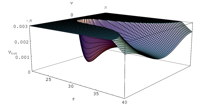
Figure 2: A detailed view of the meta-stable dS minimum of the potential $V_{\text{tot}}$.

Figs. 2 and 3 show the typical shape of $V_{\text{tot}}$ in the dS phase. Here we chose $c=-10$ and $\hat{A}_{1,m_{1}}=9867$. Fig. 2 displays the $(r,v)$-dependence of the potential, illustrating that we have indeed a meta-stable dS vacuum. Fig. 3 depicts $V_{\text{tot}}$ in the $r$-direction for $v=0$.

Figure 3: A view of $V_{\text{tot}}(r,v)$ in the $r$-direction along $v=0$.

Let us conclude this section with a remark on the periodicity of $V_{\text{tot}}$ in the $v$-direction, which arises from the oscillatory terms in $V_{\text{1-inst}}$. As discussed in subsection 4.3, this reflects the fact that at leading order in the instanton correction there is a residual symmetry arising from the broken $\beta$-shift. Strictly speaking, we then obtain an infinite number of copies of the (A)dS vacua found above. Including higher order subleading terms, however, will break this discrete symmetry completely, thereby lifting the degeneracy between these vacua. In order to decide on the fate of these vacua one would have to sum the whole instanton series, which is, however, beyond the scope of this paper. We have verified that, when performing the above analysis by taking into account the sub- and subsubleading contributions to the potential (69), one still has (for a suitable choice of integration constants) one meta-stable dS vacuum, while the other local minima generically become meta-stable AdS vacua. This analysis gives some evidence that the qualitative picture found above will remain valid after resumming the instanton series. In particular, we expect that the stabilization of the hypermultiplets will also be a feature of the complete instanton solution.

To make further progress on this issue, we have to improve our understanding on membrane instanton calculations beyond what has been done in [7, 52]. Ideally we would like to fix the numerical coefficients in our instanton expansion completely through the microscopic string theory description. For (some) more general CY₃ compactifications of the type IIA string this may be done using the duality to heterotic string theory on $K3\times T^{2}$ [53], where the hypermultiplet moduli space is classically exact in the string coupling constant. However, this duality generically involves more than one hypermultiplet, which requires a more generic setup than what is considered here. Furthermore, it would be interesting to investigate whether these coefficients have some deeper meaning in the context of topological string theory, analogous to the coefficients appearing in the D3-brane instanton corrections to orientifold compactifications of the type IIB string recently investigated in [5].

7 Discussion

Let us now discuss the relation between KKLT [1] and our set-up. In order to stabilize all moduli and to obtain a meta-stable dS vacuum, KKLT proposed a three step procedure, where first all moduli apart from the dilaton were fixed by fluxes, second the dilaton is stabilized by non-perturbative instanton effects at an AdS vacuum, and finally a positive energy contribution (in form of anti-D3-branes) is added to lift this vacuum to a meta-stable dS vacuum. When including a space-filling RR 3-form flux in our case, the classical potential is positive definite and of runaway type. There is no vacuum, except the one at vanishing string coupling, and both RR scalars correspond to flat directions. This does not change when the perturbative corrections to the universal hypermultiplet found in [10] are included. The picture changes completely when taking into account the leading membrane instanton corrections to the universal hypermultiplet. These corrections to the scalar metric lift the flat directions corresponding to the RR scalars, so that all the present moduli are fixed by the potential. Furthermore, by making a suitable choice of the numerical parameters corresponding to the one-loop determinant around a one-instanton background, the moduli can be stabilized in a meta-stable dS vacuum at small string coupling $g_{s}\ll 1$. Here, the appearance of the dS vacuum does not require to add a positive energy contribution (like anti-D3-branes) by hand, as this contribution is already provided by the background flux when taking the perturbative corrections to the hypermultiplet geometry into account. This picture is completely analogous to the one obtained for type the IIB orientifold compactifications studied in [4] where it was found that the leading order $\alpha^{\prime}$ corrections to the Kähler potential together with the leading D3-brane instanton correction can also give rise to meta-stable dS vacua without the need of adding an additional positive energy contribution. On phenomenological grounds, it would be interesting to analyze the stability and lifetime of these dS vacua along the lines of [1].

In our model we have truncated the vector multiplets that arise in a realistic compactification of type IIA strings on a rigid Calabi-Yau manifold. In order to address the issue of stabilizing these moduli as well, it would be necessary to include them in the effective action. This is, however, beyond the scope of the present paper. In this context, let us remark that including these vector multiplets (whose scalar fields correspond to the complexified Kähler moduli of the compactification) also allows to consider more general fluxes, like e.g. 2- and 4-form fluxes related to the even homology cycles of the rigid Calabi-Yau manifold, which could then be used to stabilize these moduli as well. Previous investigations on this topic indicate that these moduli will likely be stabilized at special points of the Kähler moduli space where the Calabi-Yau geometry degenerates (as e.g. at conifold points), either through fluxes [54] or non-perturbative effects arising from (Lorentzian) branes wrapping the degenerate cycles [55]. In this context it is also interesting to note that instanton corrections of the type discussed in this paper play an important role in a proper understanding of string theory at these degeneration points [7, 14]. It would therefore be highly desirable to extend the present analysis to include vector multiplets.

Possible extensions of the present work would be to include also fivebrane instanton corrections to the universal hypermultiplet. Some results were already obtained in [12], and it would be challenging to combine them with the results obtained in this paper. Another direction to pursue is to consider more generic Calabi-Yau threefolds, in which one also has additional hypermultiplets. The quaternion-Kähler manifold would then be higher dimensional, and it would be interesting to study instanton effects in this context and see how they stabilize all the complex structure moduli. We leave this open for future research.

Appendix A Notation and conventions

In order to study the scalar potential in gauged supergravity, we need to fix the conventions and normalizations of the various quaternionic quantities. We mainly follow the notation of [56, 57, 58], but with a few modifications on the conventions mentioned explicitly below.

A.1 General properties of quaternion-Kähler geometry

The quaternionic structure is normalized such that

$$J^{\Lambda}J^{\Sigma}=-\delta^{\Lambda\Sigma}-\varepsilon^{\Lambda\Sigma\Pi}J^{\Pi}\ ,$$ (70)

with $\Lambda,\Sigma,\Pi=1,2,3$. There exist quaternionic 1-form vielbeine $V_{i}^{\alpha}$, in terms of which the line element reads

$$\mathrm{d}s^{2}=G_{AB}\,\mathrm{d}\phi^{A}\otimes\mathrm{d}\phi^{B}=G_{\bar{\alpha}\beta}V_{i}^{\beta}\otimes\bar{V}^{i\bar{\alpha}}\ .$$ (71)

Here, $G_{AB}$ is the quaternionic metric, $\bar{V}^{i\bar{\alpha}}$ is the complex conjugate of $V_{i}^{\alpha}$, and $G_{\bar{\alpha}\beta}$ is the tangent space metric that appears in front of the kinetic terms of the fermions. The quaternionic 2-forms can then be written as

$$J^{\Lambda}=\frac{\mathrm{i}}{2}\,G_{\bar{\alpha}\beta}V_{i}^{\beta}\wedge\bar{V}^{j\bar{\alpha}}(\tau^{\Lambda})^{i}{}_{j}\ ,$$ (72)

where $\tau^{\Lambda}$ are the Pauli matrices. For $4n$-dimensional QK manifolds, the range of the indices is $i=1,2$, $\alpha=1,...,2n$, and $A=1,...,4n$.

Quaternion-Kähler manifolds are Einstein, and hence the Ricci tensor is proportional to the metric. Following [45], we have

$$R_{AB}=\frac{1}{4n}\,G_{AB}R\ ,$$ (73)

where $R$ is the (constant) Ricci scalar. Furthermore, there exist SU(2) connection 1-forms $\vec{\mathcal{V}}=\vec{\mathcal{V}}_{\!A}\,\mathrm{d}\phi^{A}$ with SU(2) curvature

$$\vec{\mathcal{R}}\equiv\mathrm{d}\vec{\mathcal{V}}-\tfrac{1}{2}\,\vec{\mathcal{V}}\times\vec{\mathcal{V}}\ .$$ (74)

The exterior derivative on $\vec{\mathcal{R}}$ yields the Bianchi identities

$$\mathrm{d}\vec{\mathcal{R}}=\vec{\mathcal{V}}\times\vec{\mathcal{R}}\ .$$ (75)

The relation between SU(2) curvature and quaternionic 2-forms reads

$$\vec{\mathcal{R}}=\nu\vec{J}\ ,\qquad\nu\equiv\frac{1}{4n(n+2)}\,R\ .$$ (76)

For the gauging, we need the conventions for the moment maps. They are defined from

$$\vec{J}_{AB}\,k^{B}_{I}=D_{A}\vec{P}_{I}=(\partial_{A}-\vec{\mathcal{V}}_{\!A}\times)\vec{P}_{I}\ ,$$ (77)

where $I$ labels the different isometries and $D_{A}$ is the SU(2) covariant derivative.

One can solve this relation for the moment maps to get [58]

$$\vec{P}_{I}=-\frac{1}{2n\nu}\,\vec{J}^{A}{}_{B}D_{A}k^{B}_{I}\ .$$ (78)

Notice that the right-hand side is independent of the metric, except for the factor $\nu$. Choosing this factor sets the scale of the metric, and for the universal hypermultiplet that we discuss below, we set the scale such that $\nu=-1/2$.

In supergravity, the value of $\nu$ is fixed in terms of the gravitational coupling constant. If we normalize the kinetic terms of the graviton and scalars in the supergravity action as

$$e^{-1}\mathcal{L}_{\text{kin}}=-\frac{1}{2\kappa^{2}}\,R(e)-\frac{1}{2}\,G_{AB}\partial_{\mu}\phi^{A}\,\partial^{\mu}\phi^{B}\ ,$$ (79)

then local supersymmetry fixes $\nu=-\kappa^{2}$. This is in accordance with [45], and with [6] after a rescaling of the metric $G_{AB}$ with a factor 1/2. For the universal hypermultiplet, we will work with conventions in which $\nu=-1/2$, so we set $\kappa^{2}=1/2$ below. To compare with [58], we first multiply the Lagrangian (79) by 2 and then set $\kappa^{2}=2$.

We now include the scalar potential that arises after gauging a single isometry. The isometry can then be gauged by the graviphoton and in the absence of any further vector multiplets, the relevant terms in the Lagrangian are

$$e^{-1}\mathcal{L}=-\frac{1}{2\kappa^{2}}\,R-\frac{1}{2}\,G_{AB}D_{\mu}\phi^{A}\,D^{\mu}\phi^{B}-\big{(}2\kappa^{-2}G_{AB}\,k^{A}k^{B}-3\,\vec{P}\!\cdot\!\vec{P}\,\big{)}\ .$$ (80)

Here, $D_{\mu}$ is the covariant derivative with respect to the gauged isometry that corresponds to the Killing vector $k^{A}$. The factors of $\kappa$ appear on dimensional grounds, as one can easily verify. For $\kappa^{2}=2$ this agrees precisely with the result in [58]; here, however, we set $\kappa^{2}=1/2$.

Our conventions are chosen such that they naturally apply to the universal hypermultiplet metric and the conventions used in [59]. At the classical level we have

$$\mathrm{d}s^{2}=G_{AB}\,\mathrm{d}\phi^{A}\otimes\mathrm{d}\phi^{B}=\mathrm{d}\phi^{2}+\mathrm{e}^{-\phi}(\mathrm{d}\chi^{2}+\mathrm{d}\varphi^{2})+\mathrm{e}^{-2\phi}(\mathrm{d}\sigma+\chi\mathrm{d}\varphi)^{2}\ .$$ (81)

For the corresponding Ricci tensor we find

$$R_{AB}=-\frac{3}{2}\,G_{AB}\ .$$ (82)

The Ricci scalar is then $R=-6$ and therefore we have $\nu=-1/2$. This implies that in these conventions we should set $\kappa^{2}=1/2$, which is equivalent to a cosmological constant $\Lambda=-3/2$ on the quaternion-Kähler manifold.

A.2 Quaternion-Kähler geometry of the PT metric

The quaternionic properties of the PT metric can be demonstrated by constructing the corresponding quaternionic 1-form vielbeine (71), which we parameterize as

$$V_{i}^{\alpha}=\begin{pmatrix}\bar{a}&-\bar{b}\\ b&a\end{pmatrix}\ .$$ (83)

Substituting this ansatz into (71), we obtain

$$\mathrm{d}s^{2}=a\otimes\bar{a}+b\otimes\bar{b}+\text{c.c.}\ .$$ (84)

Comparing this expression with the PT metric (7), we can choose

$$a=\frac{1}{\sqrt{2\,}\,r}\,\big{(}f^{1/2}\,\mathrm{d}r+\mathrm{i}f^{-1/2}\,(\mathrm{d}t+\Theta)\big{)}\ ,\qquad b=\frac{1}{\sqrt{2\,}\,r}\,(f\mathrm{e}^{h})^{1/2}\,\big{(}\mathrm{d}u+\mathrm{i}\,\mathrm{d}v\big{)}\ .$$ (85)

The computation of the quaternionic 2-forms (72) then yields

$$J^{1}=-\mathrm{i}(a\wedge b-\bar{a}\wedge\bar{b})\ ,\quad J^{2}=a\wedge b+\bar{a}\wedge\bar{b}\ ,\quad J^{3}=-\mathrm{i}(a\wedge\bar{a}+b\wedge\bar{b})\ .$$ (86)

These satisfy the quaternionic algebra (70).

Using (76) and (75), we then determine the SU(2) connection for the PT metric,

$$\mathcal{V}^{1}=\frac{1}{r}\,\mathrm{e}^{h/2}\mathrm{d}v\ ,\qquad\mathcal{V}^{2}=\frac{1}{r}\,\mathrm{e}^{h/2}\mathrm{d}u\ ,$$

$$\mathcal{V}^{3}=-\frac{1}{2r}\,(\mathrm{d}t+\Theta)-\frac{1}{2}\,(\partial_{v}h\,\mathrm{d}u-\partial_{u}h\,\mathrm{d}v)\ .$$ (87)

The PT metric has a shift symmetry in $t$. In coordinates $(r,u,v,t)$ the corresponding Killing vector is given by

$$k^{A}=(\,0\,,\,0\,,\,0\,,\,e_{0}\,)^{\mathrm{T}}\ .$$ (88)

The moment maps of this shift symmetry can be computed from (78). The result is independent of the functions $f$, $h$, and $\Theta$ and reads

$$P^{1}=0\ ,\qquad P^{2}=0\ ,\qquad P^{3}=\frac{e_{0}}{r}\ .$$ (89)

A.3 The 4-fermion coupling of the PT metric

In order to make contact with the string calculation of [7], we need to construct the symmetric tensor $\mathcal{W}_{\alpha\beta\gamma\delta}$, which appears in the four-fermion term. This can be done along the lines outlined in [45]. Note that the tensor $\Omega_{XYZW}$ appearing in Bagger and Witten [6] is totally symmetric for rigid supersymmetry, but not in the supergravity case.

The symmetric tensor $\mathcal{W}_{\alpha\beta\gamma\delta}$ can be obtained from the curvature decomposition

$$R_{ABCD}=\nu(R^{\mathrm{SU}(2)})_{ABCD}+\frac{1}{2}\,{L_{DC}}^{\alpha\beta}\,\mathcal{W}_{\alpha\beta\gamma\delta}\,{L_{AB}}^{\gamma\delta}\ .$$ (90)

Here,

$$(R^{\mathrm{SU}(2)})_{ABCD}=\frac{1}{2}\,g_{D[A}\,g_{B]C}+\frac{1}{2}\,J^{\Lambda}_{AB}\,J^{\Lambda}_{DC}-\frac{1}{2}\,J^{\Lambda}_{D[A}\,J_{B]C}^{\Lambda}\ ,$$ (91)

and

$${L_{AB\alpha}}^{\beta}=V_{Ai\alpha}\,\bar{V}^{i\beta}_{B}\ .$$ (92)

Eq. (90) can be solved for $\mathcal{W}_{\alpha\beta\gamma\delta}$ by using the inverse relation for ${L_{AB}}^{\alpha\beta}$:

$$-\frac{1}{2}\,V^{iB}_{\gamma}\,V^{A}_{i\delta}\,{L_{AB}}^{\alpha\beta}=\delta^{\alpha}_{\gamma}\,\delta^{\beta}_{\delta}\ .$$ (93)

The resulting expression for $\mathcal{W}_{\alpha\beta\gamma\delta}$ then reads:

$$\mathcal{W}_{\alpha\beta\gamma\delta}=\frac{1}{2}\,\epsilon^{ij}\epsilon^{kl}\,V_{i\delta}^{A}\,V_{j\gamma}^{B}\,V_{k\beta}^{D}\,V_{l\alpha}^{C}\big{(}R_{ABCD}-\nu(R^{\mathrm{SU}(2)})_{ABCD}\big{)}\ .$$ (94)

The components of $\mathcal{W}_{\alpha\beta\gamma\delta}$ can now be obtained by calculating $R_{ABCD}$ for the PT metric (7) and substituting the expressions for the vielbeins and complex structures obtained above in the corresponding definitions. In order to write the independent components of $\mathcal{W}_{\alpha\beta\gamma\delta}$ in a compact way, it is useful to introduce the complex variable $z=u+\mathrm{i}v$. The result is given in (3.2).

Appendix B Tensor multiplet description

Consider the hypermultiplet Lagrangian based on the PT metric (7). It is interesting to write down the $N=2$ tensor multiplet Lagrangian obtained after dualizing the scalar $t$ into a 2-form gauge potential with field strength $H_{\mu\nu\rho}$. Using the results of [59], this Lagrangian can easily be read off,

$$\mathcal{L}_{T}=\frac{1}{2}\,r^{2}fH_{\mu}H^{\mu}-\frac{1}{2}\,\mathcal{G}_{AB}\,\partial_{\mu}\phi^{A}\,\partial^{\mu}\phi^{B}-\Theta_{A}H^{\mu}\partial_{\mu}\phi^{A}\ .$$ (95)

Here, $\Theta_{A}$ are the three components of the one-form defined in (10), and $\mathcal{G}_{AB}$ is the metric on the manifold spanned by the three scalars $(r,u,v)$. The line element can be written as

$$\mathrm{d}s^{2}=\frac{f}{r^{2}}\,\Big{[}\mathrm{d}r^{2}+\mathrm{e}^{h}\big{(}\mathrm{d}u^{2}+\mathrm{d}v^{2}\big{)}\Big{]}\ ,$$ (96)

where $\mathrm{e}^{h}$ satisfies the Toda equation and $f(r,u,v)$ the constraint (9). This 3-dimensional geometry is related to Einstein-Weyl spaces, as explained in [38].

Appendix C Details of the Toda solution

This appendix collects several technical details about the solution of the Toda equation constructed in section 4. We start by proving $m_{n}\geq-2$ in subsection C.1, while the proof for $\alpha=0$ is given in subsection C.2. The derivation of the one-instanton solution is given in subsection C.3.

C.1 The lower bound on $m_{n}$

In this subsection we establish $m_{n}\geq-2$. Our starting point is the ansatz (17), which we substitute into the Toda equation (21). This results in the following power series expansion

$$0= \sum_{n,m}r^{-m/2+\alpha+1}\,\mathrm{e}^{-2n\sqrt{r}}\big{[}(\Delta+n^{2})f_{n,m}+(n\,a_{m+1}\,r^{-1/2}+b_{m+2}\,r^{-1})f_{n,m}\big{]}$$

$$+\sum_{n,m}\sum_{n^{\prime},m^{\prime}}r^{-(m+m^{\prime})/2+2\alpha}\,\mathrm{e}^{-2(n+n^{\prime})\sqrt{r}}\,\big{[}f_{n^{\prime},m^{\prime}}(\Delta+2n^{2})f_{n,m}$$

$$\mspace{128.0mu}-\nabla f_{n,m}\cdot\nabla f_{n^{\prime},m^{\prime}}+2(a_{m+1}\,r^{-1/2}+b_{m+2}\,r^{-1})f_{n,m}\,f_{n^{\prime},m^{\prime}}\big{]}$$

$$+\sum_{n,m}\sum_{n^{\prime},m^{\prime}}\sum_{n^{\prime\prime},m^{\prime\prime}}r^{-(m+m^{\prime}+m^{\prime\prime})/2+3\alpha-1}\,\mathrm{e}^{-2(n+n^{\prime}+n^{\prime\prime})\sqrt{r}}f_{n,m}\,f_{n^{\prime},m^{\prime}}\,f_{n^{\prime\prime},m^{\prime\prime}}$$

$$\mspace{128.0mu}\times\big{[}n^{2}+n\,a_{m+1}\,r^{-1/2}+b_{m+2}\,r^{-1}\big{]}\ ,$$ (97)

where we have extended the definitions for $a_{m}$, $b_{m}$ given in (23) to non-zero $\alpha$:

$$a_{m}=\tfrac{1}{2}\,(2m-4\alpha-1)\ ,\qquad b_{m}=\tfrac{1}{4}\,(m-2\alpha)(m-2\alpha-2)\ .$$ (98)

In order to obtain a bound on $m_{n}$ (for which the $f_{n,m_{n}}\neq 0$), we extract the leading order contributions in the $r$-expansion arising from the single, double and triple sum in (C.1). Starting at $n=1$ and working iteratively towards higher values $n=2,3,\ldots$, we find that at a fixed value of $n$ these contributions are proportional to

single sum $$\propto\ r^{-m_{n}/2+\alpha+1}$$

double sum $$\propto\ r^{-m_{n}+2\alpha}$$

triple sum $$\propto\ r^{-3m_{n}/2+3\alpha-1}\ .$$ (99)

Investigating the $m_{n}$-dependence of these relations, we find that for $m_{n}\leq-3$ the leading order term in $r$ arises from the triple sum, which decouples from all the other terms in (C.1).

We now assume that for a fixed value $n$ there exsists an $f_{n,m_{n}}\neq 0$ for $m_{n}\leq-3$. Extracting the equation leading in $r$ from (C.1), we find that

$$n^{2}\,f^{3}_{n,m_{n}}=0\ ,\qquad m_{n}\leq-3\ ,$$ (100)

which has $f_{n,m_{n}}=0$ as its only solution. Hence, we establish the lower bound

$$m_{n}\geq-2$$ (101)

for all values of $n$ or, equivalently, all instanton sectors.

C.2 Fixing the parameter $\alpha$

When making the ansatz (17) in order to describe membrane instanton corrections to the universal hypermultiplet, we included the parameter $\alpha\in[0,1/2[$ to allow for the possibility that the leading term in the instanton solution occurs with a fractional power of $g_{s}$. Based on the plausible assumption that the perturbation series around the instanton gives rise to a power series in $g_{s}$ (and not fractional powers thereof) we now give a proof that a consistent solution of the Toda equation requires $\alpha=0$.

Splitting (C.1) into instanton sectors gives us the following analogue of (4)

$$0=\sum_{n,m} \ r^{-m/2+\alpha}\,\mathrm{e}^{-2n\sqrt{r}}\,\Big{\{}(\Delta+n^{2})\,f_{n,m+2}+n\,a_{m+2}\,f_{n,m+1}+b_{m+2}\,f_{n,m}$$

$$+\sum_{n^{\prime},m^{\prime}}r^{\alpha}\,\mathrm{e}^{-2n^{\prime}\!\sqrt{r}}\,\big{[}\,2n\,a_{m^{\prime}+1}\,f_{n^{\prime},m-m^{\prime}-1}+2b_{m^{\prime}+2}\,f_{n^{\prime},m-m^{\prime}-2}$$

$$\mspace{134.0mu}+f_{n^{\prime},m-m^{\prime}}\,(\Delta+2n^{2})-\nabla f_{n^{\prime},m-m^{\prime}}\cdot\nabla\big{]}f_{n,m^{\prime}}$$

$$+\sum_{n^{\prime},m^{\prime}}\sum_{n^{\prime\prime},m^{\prime\prime}}r^{2\alpha}\,\mathrm{e}^{-2(n^{\prime}+n^{\prime\prime})\sqrt{r}}\,f_{n,m^{\prime}}f_{n^{\prime},m^{\prime\prime}}\,\big{[}n^{2}f_{n^{\prime\prime},m-m^{\prime}-m^{\prime\prime}-2}$$

$$\mspace{94.0mu}+n\,a_{m^{\prime}+1}\,f_{n^{\prime\prime},m-m^{\prime}-m^{\prime\prime}-3}+b_{m^{\prime}+2}\,f_{n^{\prime\prime},m-m^{\prime}-m^{\prime\prime}-4}\big{]}\Big{\}}\,.$$ (102)

Based on this equation we can now make several observations. First, we find that the $N=1$ sector of (C.2) still gives rise to (24), with the coefficients $a_{m}$, $b_{m}$ now replaced by (98). To lowest order, $m=m_{1}$, this is just the equation

$$(\Delta+1)f_{1,m_{1}}(u,v)=0\ .$$ (103)

Second, we observe that the equation describing the $N=2$ sector is modified to

$$0 =(\Delta+4)\,f_{2,m}+2a_{m}\,f_{2,m-1}+b_{m}\,f_{2,m-2}$$

$$\quad\,+\sum_{m^{\prime}}r^{\alpha}\big{[}f_{1,m-m^{\prime}-2}+a_{m^{\prime}+1}\,f_{1,m-m^{\prime}-3}+b_{m^{\prime}+2}\,f_{1,m-m^{\prime}-4}-\nabla f_{1,m-m^{\prime}-2}\cdot\nabla\big{]}f_{1,m^{\prime}}\ .$$

Note that for $\alpha=0$ the sum appearing in the second line is just an inhomogeneous term to the equations determining $f_{2,m}$. For $\alpha\neq 0$, however, the sum decouples due to the different powers in $r$. Therefore, in the case $\alpha\neq 0$, the sum gives rise to an additional constraint equation, which is absent for $\alpha=0$. Since the sum contains the $f_{1,m}$ only, this additional relation imposes a restriction on the $N=1$ instanton solution. Upon using (103), this additional constraint reads, at the lowest level,

$$f_{1,m_{1}}^{2}-(\nabla f_{1,m_{1}})^{2}=0\ .$$ (104)

For $\alpha\neq 0$ a non-trivial 1-instanton solution has to satisfy both (103) and (104), so that for establishing $\alpha=0$ it suffices to show that these equations have no common non-trivial solution:

Suppose that $f_{1,m_{1}}\neq 0$, which by definition of $f_{1,m_{1}}$ has to hold. We then multiply (103) with $f_{1,m_{1}}$, giving

$$0=f_{1,m_{1}}\,\Delta f_{1,m_{1}}+f_{1,m_{1}}^{2}=f_{1,m_{1}}\,\Delta f_{1,m_{1}}+(\nabla f_{1,m_{1}})^{2}=\tfrac{1}{2}\Delta f^{2}_{1,m_{1}}\ ,$$

where we have used (104) in the first step. In terms of complex coordinates $z=u+\mathrm{i}v$ it is $\Delta=4\partial_{z}\partial_{\bar{z}}$, and the general solution reads

$$f_{1,m_{1}}^{2}(z,\bar{z})=g(z)+\bar{g}(\bar{z})\ .$$

Substituting this back into (103), we find

$$0=(\Delta+1)f_{1,m_{1}}=f_{1,m_{1}}^{-3}\big{[}\!-\partial_{z}g(z)\,\partial_{\bar{z}}\bar{g}(\bar{z})+(g(z)+\bar{g}(\bar{z}))^{2}\big{]}\ ,$$

which is equivalent to

$$\partial_{z}g(z)\,\partial_{\bar{z}}\bar{g}(\bar{z})=g(z)^{2}+2g(z)\bar{g}(\bar{z})+\bar{g}(\bar{z})^{2}\ .$$

Since the right-hand side of this expression contains terms which are (anti-) holomorphic, whereas the left-hand side does not, we find that the only solution is given by $g(z)=\mathrm{i}c$ with $c\in\fieldR$ constant. Thus $f_{1,m_{1}}=0$, which contradicts our assumption and shows that the ansatz (17) does not give rise to a one-instanton sector if $\alpha\neq 0$. Conversely, a non-trivial one-instanton sector exists for $\alpha=0$ only, which then fixes $\alpha=0$.

C.3 The one-instanton solution

The general one-dimensional solution in the one-instanton sector was given in (25). The functions $G_{s}(x)$ introduced there are defined by

$$G_{s}(x)=x^{s+1}h_{s-1}(x)\ ,$$ (105)

where $h_{s}(x)=j_{s}(x)+\mathrm{i}y_{s}(x)$ are the spherical Bessel functions of the third kind. For $s\geq 0$ the $G_{s}(x)$ have no poles. Explicitly, they read

$$G_{0}(x)=\mathrm{e}^{\mathrm{i}x}\ ,\qquad G_{s>0}(x)=2^{-s}\,\mathrm{e}^{\mathrm{i}x}\,\sum_{k=1}^{s}\frac{(2s-k-1)!}{(s-k)!\,(k-1)!}\,(-2\mathrm{i}x)^{k}\ .$$ (106)

Using the properties

$$x^{2}h_{s}^{\prime\prime}+2x\,h_{s}^{\prime}+\big{[}x^{2}-s(s+1)\big{]}h_{s}=0\ ,\qquad h_{s}^{\prime}+\frac{s+1}{x}\,h_{s}=h_{s-1}\ ,$$ (107)

we easily verify the relation

$$(\partial_{x}^{2}+1)\,G_{s}(x)=2s\,G_{s-1}(x)\ .$$ (108)

The proof of (25) is now simple:

$$(\partial_{x}^{2}+1)f_{1,m}(x) =\operatorname{\mathrm{Re}}\sum_{s\geq 0}\,\frac{1}{s!\,(-2)^{s}}\,k_{1,m}(s)\,(\partial_{x}^{2}+1)G_{s}(x)$$

$$=-\operatorname{\mathrm{Re}}\sum_{s\geq 1}\,\frac{1}{(s-1)!\,(-2)^{s-1}}\,k_{1,m}(s)\,G_{s-1}(x)$$

$$=-\operatorname{\mathrm{Re}}\sum_{s\geq 0}\,\frac{1}{s!\,(-2)^{s}}\,k_{1,m}(s+1)\,G_{s}(x)$$

$$=-\operatorname{\mathrm{Re}}\sum_{s\geq 0}\,\frac{1}{s!\,(-2)^{s}}\,\big{[}a_{m}k_{1,m-1}(s)+b_{m}k_{1,m-2}(s)\big{]}\,G_{s}(x)$$

$$=-\,a_{m}f_{1,m-1}(x)-b_{m}f_{1,m-2}(x)\ .$$ (109)

For the general $(u,v)$-dependent solution given in (28), the proof is almost identical.

References

- [1] S. Kachru, R. Kallosh, A. Linde and S. Trivedi, de Sitter vacua in string theory. Phys. Rev. D 68 (2003) 046005, hep-th/0301240.
- [2] E. Silverstein, TASI/PiTP/ISS lectures on moduli and microphysics. hep-th/0405068.
-
[3]
C. Escoda, M. Gomez-Reino and F. Quevedo, Saltatory de Sitter
string vacua. J. High Energy Phys. 11 (2003) 065, hep-th/0307160;
S. Kachru, R. Kallosh, A. Linde, J. Maldacena, L. McAllister and S. P. Trivedi, Towards inflation in string theory. JCAP 0310 (2003) 013, hep-th/0308055;
C.P. Burgess, R. Kallosh and F. Quevedo, de Sitter string vacua from supersymmetric D-terms. J. High Energy Phys. 10 (2003) 056, hep-th/0309187;
A. Saltman and E. Silverstein, The scaling of the no-scale potential and de Sitter model building. J. High Energy Phys. 11 (2004) 066, hep-th/0402135;
F. Denef, M.R. Douglas and B. Florea, Building a better racetrack. J. High Energy Phys. 06 (2004) 034, hep-th/0404257;
J.J. Blanco-Pillado, C.P. Burgess, J.M. Cline, C. Escoda, M. Gomez-Reino, R. Kallosh, A. Linde and F. Quevedo, Racetrack inflation. J. High Energy Phys. 11 (2004) 063, hep-th/0406230;
V. Balasubramanian, P. Berglund, J.P. Conlon and F. Quevedo, Systematics of moduli stabilisation in Calabi-Yau flux compactifications. J. High Energy Phys. 03 (2005) 007, hep-th/0502058;
F. Denef, M. Douglas, B. Florea, A. Grassi and S. Kachru, Fixing all moduli in a simple F-theory compactification. hep-th/0503124;
P. S. Aspinwall and R. Kallosh, Fixing all moduli for M-theory on . hep-th/0506014. - [4] V. Balasubramanian and P. Berglund, Stringy corrections to Kaehler potentials, SUSY breaking, and the cosmological constant problem. J. High Energy Phys. 11 (2004) 085, hep-th/0408054.
- [5] P. Berglund and P. Mayr, Non-perturbative superpotentials in F-theory and string duality. hep-th/0504058.
- [6] J. Bagger and E. Witten, Matter couplings in N=2 supergravity. Nucl. Phys. B 222 (1983) 1.
- [7] K. Becker, M. Becker and A. Strominger, Five-branes, membranes and nonperturbative string theory. Nucl. Phys. B 456 (1995) 130, hep-th/9507158.
- [8] K. Becker and M. Becker, Instanton action for type II hypermultiplets. Nucl. Phys. B 551 (1999) 102, hep-th/9901126.
-
[9]
S. Cecotti, S. Ferrara and L. Girardello, Geometry of type II
superstrings and the moduli of superconformal field theories.
Int. J. Mod. Phys. A 4 (1989) 2475;
S. Ferrara and S. Sabharwal, Quaternionic manifolds for type II superstring vacua of Calabi-Yau spaces. Nucl. Phys. B 332 (1990) 317. - [10] I. Antoniadis, R. Minasian, S. Theisen and P. Vanhove, String loop corrections to the universal hypermultiplet. Class. and Quant. Grav. 20 (2003) 5079, hep-th/0307268.
- [11] L. Anguelova, M. Roček and S. Vandoren, Quantum corrections to the universal hypermultiplet and superspace. Phys. Rev. D 70 (2004) 066001, hep-th/0402132.
- [12] M. Davidse, U. Theis and S. Vandoren, Fivebrane instanton corrections to the universal hypermultiplet. Nucl. Phys. B 697 (2004) 48, hep-th/0404147.
- [13] B.R. Greene, D.R. Morrison, C. Vafa, A geometric realization of confinement. Nucl. Phys. B 481 (1996) 513, hep-th/9608039.
- [14] H. Ooguri and C. Vafa, Summing up D-Instantons, Phys. Rev. Lett. 77 (1996) 3296, hep-th/9608079.
- [15] P. Aspinwall, Compactification, geometry and duality: N=2. In “Boulder 1999, Strings, branes and gravity”, 723. hep-th/0001001.
- [16] M. Gutperle and M. Spalinski, Supergravity instantons and the universal hypermultiplet. J. High Energy Phys. 06 (2000) 037, hep-th/0005068; Supergravity instantons for hypermultiplets. Nucl. Phys. B 598 (2001) 509, hep-th/0010192.
- [17] U. Theis and S. Vandoren, Instantons in the double-tensor multiplet. J. High Energy Phys. 09 (2002) 059, hep-th/0208145.
- [18] M. Davidse, M. de Vroome, U. Theis and S. Vandoren, Instanton solutions for the universal hypermultiplet. Fortschr. Phys. 52 (2004) 708, hep-th/0309220.
- [19] K. Behrndt and S. Mahapatra, De Sitter vacua from gauged supergravity. J. High Energy Phys. 01 (2004) 068, hep-th/0312063.
- [20] V. Cortés, C. Mayer, T. Mohaupt and F. Saueressig, Special geometry of Euclidean supersymmetry. I: Vector multiplets. J. High Energy Phys. 03 (2004) 028, hep-th/0312001.
- [21] V. Cortés, C. Mayer, T. Mohaupt and F. Saueressig, Special geometry of Euclidean supersymmetry. II: Hypermultiplets and the c-map. hep-th/0503094.
- [22] S. V. Ketov, Gravitational dressing of D-instantons. Phys. Lett. B 504 (2001) 262, hep-th/0010255; Quantum geometry of the universal hypermultiplet. Fortschr. Phys. 50 (2002) 909, hep-th/0111080.
- [23] S.V. Ketov, Summing up D-instantons in supergravity. Nucl. Phys. B 649 (2003) 365, hep-th/0209003.
- [24] P.-Y. Casteill, E. Ivanov and G. Valent, quaternionic metrics from harmonic superspace. Nucl. Phys. B 627 (2002) 403, hep-th/0110280.
-
[25]
B. de Wit and A. Van Proeyen, Potentials and symmetries of
general gauged supergravity - Yang-Mills models.
Nucl. Phys. B 245 (1984) 89;
B. de Wit, P. G. Lauwers and A. Van Proeyen, Lagrangians of supergravity - Matter systems. Nucl. Phys. B 255 (1985) 569. - [26] R. D’Auria, S. Ferrara and P. Fré, Special and quaternionic isometries: General couplings in supergravity and the scalar potential. Nucl. Phys. B 359 (1991) 705.
- [27] L. Andrianopoli, M. Bertolini, A. Ceresole, R. D’Auria, S. Ferrara, P. Fré and T. Magri, supergravity and super Yang-Mills theory on general scalar manifolds: Symplectic covariance, gaugings and the momentum map. J. Geom. Phys. 23 (1997) 111, hep-th/9605032.
- [28] J. Louis and A. Micu, Type II theories compactified on Calabi-Yau threefolds in the presence of background fluxes. Nucl. Phys. B 635 (2002) 395, hep-th/0202168.
- [29] S. Kachru and A. K. Kashani-Poor, Moduli potentials in type IIA compactifications with RR and NS flux. J. High Energy Phys. 03 (2005) 066, hep-th/0411279.
- [30] P. Fré, M. Trigiante and A. Van Proeyen, Stable de Sitter vacua from N=2 supergravity. Class. and Quant. Grav. 19 (2002) 4167, hep-th/0205119.
-
[31]
G. Curio and A. Krause, G-fluxes and non-perturbative
stabilisation of heterotic M-theory. Nucl. Phys. B 643 (2002) 131,
hep-th/0108220;
E.I. Buchbinder and B.A. Ovrut, Vacuum stability in heterotic M-theory. Phys. Rev. D 69 (2004) 086010, hep-th/0310112;
R. Brustein and S. P. de Alwis, Moduli potentials in string compactifications with fluxes: Mapping the discretuum. Phys. Rev. D 69 (2004) 126006, hep-th/0402088;
M. Becker, G. Curio and A. Krause, De Sitter vacua from heterotic M-theory. Nucl. Phys. B 693 (2004) 223, hep-th/0403027;
E.I. Buchbinder, Raising anti de Sitter vacua to de Sitter vacua in heterotic M-theory. Phys. Rev. D 70 (2004) 066008, hep-th/0406101. -
[32]
S. Ferrara and S. Sabharwal, Dimensional reduction of type II
superstrings. Class. and Quant. Grav. 6 (1989) L77;
M. Bodner, A. Cadavid and S. Ferrara, (2,2) Vacuum configurations for type IIA superstrings: supergravity Lagrangians and algebraic geometry. Class. and Quant. Grav. 8 (1991) 789. - [33] B. de Wit, M. Roček and S. Vandoren, Hypermultiplets, hyperkähler cones and quaternionic-kähler geometry. J. High Energy Phys. 02 (2001) 039, hep-th/0101161.
- [34] M. Przanowski, Killing vector fields in self-dual, Euclidean Einstein spaces with . J. Math. Phys. 32 (1991) 1004.
- [35] K.P. Tod, in Geometry and Physics (Aarhus 1995), pp. 307-312, Lecture Notes in Pure and Appl. Math. 184, Dekker, New York, 1997.
- [36] C. Boyer and J. Finley, Killing vectors in self-dual, Euclidean Einstein spaces. J. Math. Phys. 23 (1982) 1126.
- [37] C. Lebrun, H-space with a cosmological constant. Proc. Roy. Soc. London A380 (1982) 171.
- [38] R. Ward, Einstein-Weyl spaces and Toda fields. Class. and Quant. Grav. 7 (1990) L95.
- [39] D.M.J. Calderbank and P. Tod, Einstein metrics, hypercomplex structures and the Toda field equation. Differ. Geom. Appl. 14 (2001) 199, math.DG/9911121.
- [40] I. Bakas and K. Sfetsos, Toda fields of SO(3) hyper-Kahler metrics and free field realizations. Int. J. Mod. Phys. A 12 (1997) 2585, hep-th/9604003.
- [41] M. Aganagic, R. Dijkgraaf, A. Klemm, M. Mariño and C. Vafa, Topological strings and integrable hierarchies. hep-th/0312085.
-
[42]
S. Alexandrov, V. Kazakov and D. Kutasov, Non-perturbative effects
in matrix models and D-branes. J. High Energy Phys. 09 (2003) 057, hep-th/0306177;
S. Alexandrov and I. Kostov, Time-dependent backgrounds and non-perturbative effects. J. High Energy Phys. 02 (2005) 023, hep-th/0412223. - [43] H. Lin, O. Lunin and J. Maldacena, Bubbling AdS space and 1/2 BPS geometries. J. High Energy Phys. 10 (2004) 025, hep-th/0409174.
-
[44]
D. Joyce, Lectures on Calabi-Yau and special Lagrangian geometry.
math.DG/0108088;
J.P. Gauntlett, Branes, calibrations and supergravity. hep-th/0305074. -
[45]
E. Bergshoeff, S. Cucu, T. De Wit, J. Gheerardyn,
S. Vandoren and A. Van Proeyen, The map between conformal
hypercomplex/hyper-Kähler and quaternionic(-Kähler) geometry.
hep-th/0411209;
E. Bergshoeff, S. Cucu, T. De Wit, J. Gheerardyn, R. Halbersma, S. Vandoren and A. Van Proeyen, Superconformal N=2, D=5 matter with and without actions. J. High Energy Phys. 10 (2002) 045, hep-th/0205230. - [46] S. Gurrieri, J. Louis, A. Micu and D. Waldram, Mirror symmetry in generalized Calabi-Yau compactifications. Nucl. Phys. B 654 (2003) 61, hep-th/0211102.
- [47] R. Kallosh, A. K. Kashani-Poor and A. Tomasiello, Counting fermionic zero modes on M5 with fluxes. hep-th/0503138.
- [48] K. Behrndt, Stabilization of moduli by fluxes. AIP Conf. Proc. 743 (2005) 251, hep-th/0503129.
-
[49]
N. Seiberg and E. Witten, Gauge dynamics and compactification
to three dimensions. In The mathematical beauty of physics,
p. 333, Eds. J.M. Drouffe and J.-B. Zuber (World Scient., 1997),
hep-th/9607163;
G. Chalmers and A. Hanany, Three-dimensional gauge theories and monopoles. Nucl. Phys. B 489 (1997) 223, hep-th/9611063. -
[50]
N. Dorey, V.V. Khoze, M.P. Mattis, D. Tong and S. Vandoren,
Instantons, three-dimensional gauge theory, and the
Atiyah-Hitchin manifold. Nucl. Phys. B 514 (1998) 553, hep-th/9703228;
C. Fraser and D. Tong, Instantons, three-dimensional gauge theories, and monopole moduli spaces. Phys. Rev. D 58 (1998) 085001, hep-th/9710098;
N. Dorey, D. Tong and S. Vandoren, Instanton effects in three-dimensional supersymmetric gauge theories with matter. J. High Energy Phys. 04 (1998) 005, hep-th/9803065. - [51] P. Candelas, E. Derrick and L. Parkes, Generalized Calabi-Yau manifolds and the mirror of a rigid manifold. Nucl. Phys. B 407 (1993) 115, hep-th/9304045.
- [52] J. Harvey and G. Moore, Superpotentials and membrane instantons. hep-th/9907026.
- [53] S. Ferrara, J. A. Harvey, A. Strominger and C. Vafa, Second quantized mirror symmetry. Phys. Lett. B 361 (1995) 59, hep-th/9505162.
- [54] G. Curio, A. Klemm, D. Lüst and S. Theisen, On the vacuum structure of type II string compactifications on Calabi-Yau spaces with H-fluxes. Nucl. Phys. B 609 (2001) 3, hep-th/0012213.
-
[55]
M. Brändle and A. Lukas, Flop transitions in M-theory cosmology.
Phys. Rev. D 68 (2003) 024030, hep-th/0212263.
L. Järv, T. Mohaupt and F. Saueressig, M-theory cosmologies from singular Calabi-Yau compactifications. JCAP 0402:012 (2004), hep-th/0310174.
T. Mohaupt and F. Saueressig, Dynamical conifold transitions and moduli trapping in M-theory cosmology. JCAP 0501:006 (2005), hep-th/0410273.
A. Lukas, E. Palti and P. M. Saffin, Type IIB conifold transitions in cosmology. Phys. Rev. D 71 (2005) 066001, hep-th/0411033.
T. Mohaupt and F. Saueressig, Conifold cosmologies in IIA string theory. Fortschr. Phys. 53 (2005) 522, hep-th/0501164. -
[56]
J. De Jaegher, B. de Wit, B. Kleijn and S. Vandoren, Special
geometry in hypermultiplets. Nucl. Phys. B 514 (1998) 553, hep-th/9707262;
B. de Wit, B. Kleijn and S. Vandoren, Superconformal hypermultiplets. Nucl. Phys. B 568 (2000) 475, hep-th/9909228 - [57] B. de Wit, M. Roček and S. Vandoren, Hypermultiplets, hyperkähler cones and quaternion-Kähler geometry. J. High Energy Phys. 02 (2001) 039, hep-th/0101161.
- [58] B. de Wit, M. Roček and S. Vandoren, Gauging isometries on hyperkähler cones and quaternion-Kähler manifolds. Phys. Lett. B 511 (2001) 302, hep-th/0104215.
- [59] U. Theis and S. Vandoren, supersymmetric scalar-tensor couplings. J. High Energy Phys. 04 (2003) 042, hep-th/0303048.