Gauge thresholds in the presence of oblique magnetic fluxes

Abstract:

We compute the one-loop partition function and analyze the conditions for tadpole cancellation in type I theories compactified on tori in the presence of internal oblique magnetic fields. We check open - closed string channel duality and discuss the effect of T-duality. We address the issue of the quantum consistency of the toroidal model with stabilized moduli recently proposed by Antoniadis and Maillard (AM). We then pass to describe the computation of one-loop threshold corrections to the gauge couplings in models of this kind. Finally we briefly comment on coupling unification and dilaton stabilization in phenomenologically more viable models.

1 Introduction and Summary

¿From the very beginning, Type I string theory in the presence of internal magnetic fields has offered a host of interesting effects [1, 2, 3, 4, 5, 6]. From a theoretical point of view, such models are governed by exactly solvable conformal field theories on the worldsheet. The effect of constant abelian field strengths is reflected in the change of boundary conditions for the string coordinates. As a result, perturbative analyses are reliable. From a phenomenologically point of view, magnetized pan-branes or their T-dual branes at angles are the most promising candidate to describe semirealistic string vacua that can capture the essential features of the Standard Model or some of its supersymmetric and/or grand unified extensions [7].

Turning on internal abelian magnetic fluxes reduces the rank of the CP group to the subgroup commuting with the $U(1)$ generators. Chiral fermions may arise in the spectrum and the number of generations, related to the degeneracy of the Landau levels, is a topological number that coincides with the top Chern class of the internal gauge bundle. Since particles interact with a magnetic field according to their helicity, the degeneracy between bosons and fermions is in general removed [6, 10, 11, 12]. However special configurations can preserve some supersymmetry [13, 14].

Very recently, a new mechanism for moduli stabilization has been proposed [15] based on the use of oblique magnetic fields on non-factorizable tori. Along this line of investigation, in [16] we have described the effect of arbitrary magnetic fields on toroidal compactifications of the type I superstring in various dimensions. In the case of ${\bf T}^{6}$, one can attempt the stabilization of all closed string moduli, except dilaton and axion, through the introduction of suitable oblique choices of internal abelian magnetic fluxes while preserving a common ${\cal N}=1$ supersymmetry. Unfortunately cancelling all tadpoles both in the R-R and NS-NS sector seems to be harder to achieve than originally proposed in [15]. In [16] we have also identified the tree level gauge couplings of the surviving Chan-Paton group commuting with the magnetic and thus anomalous $U(1)$’s [17].

In the present paper we would like to extend our analysis to one-loop and compute threshold corrections to the open string gauge couplings. In principle one can play with the rationally quantized values of the internal magnetic fields in order to adjust the thresholds in closely related phenomenologically viable models and make contact with low-energy inputs.

The plan of the paper is as follows. In section 2 we fill in some gaps left open in [16] and write down detailed formulae for the Annulus ${\cal A}$ and Möbius-strip ${\cal M}$ contributions to the one-loop open string partition function in the presence of internal oblique magnetic fields. As familiar from the analysis of unoriented open strings stretched between branes with ‘parallel’ magnetic fields, there are several sectors. Neutral strings connecting branes without magnetic fields preserve ${\cal N}=4$ supersymmetry and were described long ago [19, 20, 21]. Singly charged strings connecting neutral branes to magnetized branes can at most preserve ${\cal N}=2$ or ${\cal N}=1$ supersymmetry in $D=4$. Generically supersymmetry is completely broken in these sectors. When the rank of the magnetic flux is not maximal, such as in the ${\cal N}=2$ cases, open strings carry generalized zero modes which are combinations of KK momenta and windings determined by the orientation of the magnetic field wrt the fundamental cell of the torus ${\bf T}^{6}$. When the rank of the magnetic flux is maximal, such as in ${\cal N}=1$ cases, open strings carry discrete multiplicities determined by the index $I_{ab}$ of the internal Dirac operator coupled to the magnetic field. In the unoriented case there are also doubly charged strings stretched between magnetized branes and their images under world-sheet parity $\Omega$. Moreover there are dipole strings having their ends on the same (stack of) branes and thus preserving ${\cal N}=4$ supersymmetry but carrying ‘rescaled’ momenta. Finally one has dy-charged strings connecting branes with different magnetic fluxes, generically oblique wrt one another. As shown in [16], in order to determine the magnetic shifts one has to diagonalize the orthogonal matrix

$$R_{ab}=R_{a}^{q_{a}}R_{b}^{q_{b}}$$ (1)

where $q_{a},q_{b}=\pm 1$ account for the (relative) orientation of the two ends and

$$R(H)={1-H\over 1+H}\quad,$$ (2)

with $H_{\tilde{i}\tilde{j}}(F)=E_{\tilde{i}}^{i}E_{\tilde{j}}^{j}F_{ij}$ the ‘frame’ components of $F_{ij}$. We will mostly concentrate on supersymmetric configurations and derive the detailed open string spectrum. Switching to the transverse closed string channel we check consistency with the boundary state formalism [3, 2, 22] where magnetic shifts show up as phases modulating the reflection coefficients.

In section 5 we pass to consider the effect of turning on an abelian magnetic field in two of the four non-compact directions e.g.

$$F_{\mu\nu}=\delta_{[\mu}^{2}\delta_{\nu]}^{3}fQ$$ (3)

where $Q$ is one of the generator of the unbroken Chan-Paton (CP) group. Since the spacetime magnetic ’deformation’ is integrable one can easily write down the relevant contributions: ${\cal A}(f)$ and ${\cal M}(f)$. The closed string spectrum is unaltered to the order at which we work and plays no role in our analysis. Selecting the terms quadratic in $f$ (and thus in $Q$) and subtracting the IR (in the open string channel) logarithmically divergent terms responsible for their running, we present general formulae for the one-loop threshold corrections to the gauge couplings [23]. After diagonalization of the magnetic rotation matrices, our formulae look very much the same as in the case of ’parallel’ magnetic fields [24] which in turn show some similarity with standard formulae for orbifolds [23, 25]. We can thus exploit the available technology in order to write very explicit formulae for the thresholds arising from both ${\cal N}=2$ and ${\cal N}=1$ sectors. In principle the threshold corrections under consideration might be completely determined if the other closed string moduli, except for the overall dilaton dependence, were fixed, in a supersymmetric fashion, by a proper choice of internal magnetic fields following the original proposal of [15]. Unfortunately, we have not been able so far to achieve this goal in a way consistent with tadpole cancellation in the absence of orbifolds or lower dimensional $\Omega$-planes.

In section 6 we conclude with some remarks on dilaton stabilization [26, 28] and a preliminary discussion on the effect of turning on open string Wilson line moduli and their mixing with closed string moduli. We also pay some attention to other low-energy couplings most notably Yukawa couplings.

2 Toroidal compactifications with oblique magnetic fluxes

The perturbative spectrum of unoriented strings is coded in four one-loop amplitudes [29, 30, 31, 13]. Torus ${\cal T}$ and Klein-bottle ${\cal K}$ represent the contribution of the unoriented closed strings. Annulus ${\cal A}$ and Möbius strip ${\cal M}$ represent the contributions of unoriented open strings. Our aim in this section is to compute the open string partition function for toroidal compactifications in the presence of oblique magnetic fluxes.

Toroidal compactifications of type I strings without magnetic fluxes were studied long ago [19]. The role of open string Wilson lines in the ‘adjoint’ breaking of the CP group was streamlined. Rank reduction due to a quantized NS-NS antisymmetric tensor background was first pointed out and then further clarified in connection with non-commuting Wilson lines [32, 20, 21], shift orbifolds [33, 34] and exotic $\Omega$-planes [21, 35, 13]. Special features of rational points were analyzed. Last but not least, the RR emission vertex in the asymmetric superghost picture (-1/2,-3/2) was proposed that involves the RR gauge potential rather than its field strength.

Turning on magnetic fields does not change the one-loop closed string amplitudes ${\cal T}$ and ${\cal K}$ and thus the closed string spectrum to lowest order (sphere), but does affect the open string spectrum and by open-closed string duality the boundary reflection coefficients. So far only partition functions for cases with ’parallel’ fluxes have been explicitly computed, see e.g. [13, 37, 38, 39]. We will momentarily adapt and extend those results to the case of arbitrary magnetic fluxes.

2.1 Open string partition function

Let us divide the full set of branes into various stacks $N_{0}$, $N_{1}$, … and turn on constant magnetic fields on each stack except for the first ($a=0$) that we leave unmagnetized. The resulting gauge group is $SO(N_{0})\times U(N_{1})\times...$. As shown in [15], the magnetic $U(1)$’s are anomalous and the corresponding photons become massive by eating R-R axions associated to internal (1,1) forms. Henceforth we will focus on the case of ${\bf T}^{6}$ for definiteness and suppress the integration measure $\int dt/t$ as well as the (regulated) contribution of the zero modes of the four non-compact bosonic coordinates $V_{4}/(4\pi^{2}{\alpha^{\prime}}t)^{2}$.

2.2 Neutral and Dipole strings

The annulus contribution ${\cal A}_{00}$ from the completely neutral strings is the same as for toroidal compactifications without fluxes [19]

$${\cal A}_{00}={1\over 2}N_{0}^{2}{\cal Q}(0|\tau_{A})\sum_{p_{oo}\in\Lambda_{KK}}\exp(2{\pi i{\alpha^{\prime}}p_{oo}^{2}\tau_{A}})$$ (1)

where $\tau_{A}=it/2$ and

$${\cal Q}(\zeta^{I}|\tau)={1\over 2}\sum_{\alpha,\beta}c_{\alpha\beta}{\theta\left[{}^{\alpha}_{\beta}\right](0|\tau)\over\eta^{3}(\tau)}\prod_{I=1}^{3}{i\theta\left[{}^{\alpha}_{\beta}\right](\zeta^{I}|\tau)\over\theta_{1}(\zeta^{I}|\tau)}\quad,$$ (2)

with $c_{\alpha\beta}=\exp[2\pi i(\alpha+\beta)]$ implementing the GSO projection. As indicated, only KK momenta $p^{\hat{i}}_{oo}=m^{i}E^{\hat{i}}_{i}$, with $m^{i}\in Z$ (for singly wrapped branes) and $E^{\hat{i}}_{i}$ the inverse 6-bein, are allowed. For simplicity, we have set the quantized NS-NS antisymmetric tensor $B_{ij}$ and the open string Wilson lines $A_{i}^{a}$ to zero. We postpone a brief discussion on their effects to the concluding remarks.

The Möbius-strip $\Omega$ projection in this sector reads

$${\cal M}_{00}=-{1\over 2}N_{0}{\cal Q}(0|\tau_{M})\sum_{p_{oo}\in\Lambda_{KK}}\exp({2\pi i{\alpha^{\prime}}p_{oo}^{2}\tau_{A}})$$ (3)

where $\tau_{M}=\tau_{A}+1/2$ and, again, only KK momenta are allowed.

Neutral dipole strings starting and ending on the same stack $a\neq 0$ of branes suffer no magnetic mode shifts and contribute

$${\cal A}_{a\bar{a}}=N_{a}\bar{N}_{a}{\cal Q}(0|\tau_{A})\sum_{p_{a\bar{a}}\in\Lambda_{a\bar{a}}}\exp({2\pi i{\alpha^{\prime}}\tau_{A}p_{a\bar{a}}^{2}})$$ (4)

where the lattice sum is over generalized momenta $p_{a\bar{a}}$, satisfying $p_{L}=R_{a}p_{R}$, which generalizes the condition $p_{L}=p_{R}$ valid for truly neutral strings, discussed above.

2.3 Singly and doubly charged strings

Singly charged strings, connecting unmagnetized branes to magnetized ones, are easy to analyze too. The magnetic shifts read

$$\epsilon^{I}_{oa}={1\over\pi}\arctan(q_{a}h^{I}_{a})\quad,$$ (5)

where $h^{I}_{a}$ with $I=1,2,3$ are the skew eigenvalues of $H^{a}_{\hat{i}\hat{j}}=E^{i}_{\hat{i}}E^{j}_{\hat{j}}F^{a}_{ij}$ (frame components!), and turn the supersymmetric ‘character’ ${\cal Q}(0|\tau_{A})$ into ${\cal Q}(\epsilon^{I}_{oa}\tau_{A}|\tau_{A})$.

The overall multiplicity, related to the degeneracy of the Landau levels, is given by

$$I_{oa}=|W_{a}|V({\bf T}^{6})\prod_{I}q_{a}h^{I}_{a}=\prod_{I}q_{a}m_{a}^{I}$$ (6)

where $V({\bf T}^{6})$ is the ‘volume’ of ${\bf T}^{6}$ in units of $4\pi^{2}{\alpha^{\prime}}$,

$$|W_{a}|=\det\left(\partial X^{i}\over\partial\sigma^{\alpha}\right)=\prod_{I}n^{I}_{a}$$ (7)

is the integer wrapping number, and $m^{I}_{a}$ are the integer magnetic monopole numbers. Dirac quantization indeed constraints the skew eigenvalues of $(2\pi{\alpha^{\prime}})F^{a}_{ij}$ (adimensional!) to be given by $f^{I}_{a}=m_{a}^{I}/n^{I}_{a}$. If ${\bf T}^{6}=\prod_{I}{\bf T}^{2}_{(I)}$ then $V({\bf T}^{6})=\prod_{I}V_{I}$, with $V_{I}$ the ‘volume’ of ${\bf T}^{2}_{(I)}$ and $f^{I}_{a}=V_{I}h^{I}_{a}$. In any case, it is easy to prove that

$$I_{oa}=|W_{a}|V({\bf T}^{6})\prod_{I}{\sin(\pi\epsilon^{I}_{oa})\over\cos(\pi\epsilon^{I}_{oa})}=\prod_{I}\sin(\pi\epsilon^{I}_{oa})\sqrt{\det({\cal G}_{a}+{\cal F}_{a})}\quad,$$ (8)

where ${\cal G}_{a}$ and ${\cal F}_{a}$ are the induced worldvolume metric and field strength. This has a clear interpretation in the transverse channel, where it exposes the Born-Infeld (BI) action [8, 9]. The extra product of sinus turns out to cancel a similar factor coming from the $\theta_{1}$’s in the denominator.

If one or more of the $h^{I}_{a}$ are zero, i.e. $H^{a}$ has not maximal rank, the index vanishes signalling the presence of invariant subtori ${\bf T}^{2}_{u}$, skewly embedded in ${\bf T}^{6}$. The ‘unmagnetized’ directions are those fixed under $R_{a}$ and along them the open string can carry generalized momenta simultaneously satisfying $p_{L}=R_{a}^{q_{a}}p_{R}$, at the charged end, and $p_{L}=p_{R}$, at the neutral end $a=0$. Compatibility of the two conditions follows from $\det(R_{a}^{q_{a}}-1)=0$.

Generically there are tachyons in these sectors since all susy tend to be broken by the presence of the magnetic flux [6, 10, 11]. However when $\sum_{I}(\pm)_{I}\epsilon^{I}_{0a}=0$ for some choice of signs the magnetic rotation matrix $R_{a}^{q_{a}}$ belongs to an $SU(3)$ subgroup of $SO(6)$ and the sector is at least ${\cal N}=1$ supersymmetric [40, 41, 42]. If moreover one of the three mode shifts is zero, let us say $\epsilon^{u}_{0a}=0$ for $u=3$, then $\epsilon^{1}_{0a}=\pm\epsilon^{2}_{0a}$ and the sector preserves ${\cal N}=2$ susy. Thanks to some Jacobi theta function identities the annulus amplitudes vanish in both cases and read

$${\cal A}_{oa}^{{\cal N}=1}=N_{0}N_{a}I_{oa}{\cal Q}(\epsilon^{I}_{oa}\tau_{A}|\tau_{A})$$ (9)

or

$${\cal A}_{oa}^{{\cal N}=2}=N_{0}N_{a}\Lambda^{u}_{oa}I^{\perp}_{oa}{\cal Q}(\epsilon^{I}_{oa}\tau_{A}|\tau_{A})\quad,$$ (10)

where $\Lambda^{u}_{oa}$ denotes the lattice sum in the unmagnetized complex direction, and

$$I^{\perp}_{oa}=\prod_{I\neq u}q_{a}m_{a}^{I}$$ (11)

is the reduced index that counts the degenaracy of the Landau levels in the (four) transverse magnetized directions.

As mentioned above, the lattice $\Lambda^{u}_{ao}$ consists in those generalized momenta that satisfy $p_{L}=R_{a}^{q_{a}}p_{R}$ and $p_{L}=p_{R}$. For generic choices of magnetic fluxes and thus $R_{a}$ the resulting momenta are neither pure KK nor pure windings but rather mixtures of the two. The ‘unmagnetized’ directions satisfy $R_{a}u=u$ or, equivalently, $H_{a}u=0$.

Doubly charged strings connecting magnetic branes with their $\Omega$ images carry CP multiplicity $N_{a}^{2}$ or $\bar{N}_{a}^{2}$, depending on the sign of $q_{a}=q_{b}$, suffer doubled magnetic mode shifts $\epsilon^{I}_{aa}=2\epsilon^{I}_{0a}$ and appear with rescaled degeneracy of the Landau levels

$$I_{aa}=\prod_{I}2q_{a}m_{a}^{I}=8I_{oa}\quad,\quad I^{\perp}_{aa}=\prod_{I\neq u}2q_{a}m_{a}^{I}=4I^{\perp}_{oa}\quad.$$ (12)

Moreover, this sector receives a Möbius strip contribution.

For supersymmetric configurations, one has

$${\cal A}_{aa}^{{\cal N}=1}={N^{2}_{a}\over 2}8I_{oa}{\cal Q}(2\epsilon^{I}_{0a}\tau_{A}|\tau_{A})$$ (13)

or

$${\cal A}_{aa}^{{\cal N}=2}={N^{2}_{a}\over 2}4I^{\perp}_{oa}\Lambda^{u}_{oa}(\tau_{A}){\cal Q}(2\epsilon^{I}_{oa}\tau_{A}|\tau_{A})$$ (14)

where as indicated $\Lambda^{u}_{aa}=\Lambda^{u}_{oa}$ is the same as in the singly charged sector. The Möbius strip reads

$${\cal M}_{aa}^{{\cal N}=1}={N_{a}\over 2}\hat{I}_{aa}\hat{\cal Q}(2\epsilon^{I}_{0a}\tau_{A}|\tau_{M})$$ (15)

or

$${\cal M}_{aa}^{{\cal N}=2}={N_{a}\over 2}\hat{I}^{\perp}_{a}\hat{\Lambda}^{u}_{oa}(\tau_{A})\hat{\cal Q}(2\epsilon^{I}_{oa}\tau_{A}|\tau_{M})$$ (16)

where a priori $-8I_{oa}\leq\hat{I}_{aa}\leq+8I_{oa}$ and $-4I_{oa}\leq\hat{I}^{\perp}_{aa}\leq+4I_{oa}$, both with jumps of 2 units, allow for all possible (anti)symmetrizations under $\Omega$ [13]. Although in the simple toroidal models we explicitly consider $\hat{I}_{aa}={I}_{aa}=8I_{oa}$ and $\hat{I}^{\perp}_{aa}={I}^{\perp}_{a}=4I_{oa}$, turning on a non vanishing $B$ and/or (discrete) Wilson lines may change the situation [19, 31, 13].

2.4 Dy-charged strings

We are now ready to discuss the last and most subtle case of open strings strecthed between branes with oblique magnetic fields. As obvious we will recover the simpler case of parallel magnetic fields as a limit. As shown in [16], in order to compute the magnetic shifts one has to diagonalize the orthogonal matrix $R_{ab}=R_{a}^{q_{a}}R_{b}^{q_{b}}$ (in the frame basis!). For ${\bf T}^{6}$, the eigenvalues come in (three) complex conjugate pairs $\rho^{I\pm}_{ab}=\exp(\pm i2\beta^{I}_{ab})$. The magnetic shifts are then given in general by

$$\epsilon^{I}_{ab}={2\over 2\pi}\beta^{I}_{ab}\quad.$$ (17)

If $R_{a}R_{b}=R_{b}R_{a}$, the simpler abelian composition rule $\epsilon^{I}_{ab}=\epsilon^{I}_{ao}\pm\epsilon^{I}_{ob}$ applies. Only the annulus contributes to these sectors and, depending on the amount of supersymmetry preserved, reads

$${\cal A}_{ab}^{{\cal N}=1}=N_{a}\bar{N}_{b}I_{ab}{\cal Q}(\epsilon^{I}_{ab}\tau_{A}|\tau_{A})$$ (18)

for ${\cal N}=1$ sectors, where

$$I_{ab}=C_{3}({\cal E}_{a}^{q_{a}}\otimes{\cal E}_{b}^{q_{b}})={W_{a}W_{b}\over 3!(2\pi)^{3}}\int_{{\bf T}^{6}}(q_{a}F_{a}+q_{b}F_{b})^{3}\quad,$$ (19)

and

$${\cal A}_{ab}^{{\cal N}=2}=N_{a}\bar{N}_{b}I^{\perp}_{ab}\Lambda^{u}_{ab}(it){\cal Q}(\epsilon^{I}_{oa}\tau_{A}|\tau_{A})$$ (20)

for ${\cal N}=2$ sectors, where

$$I^{\perp}_{ab}=C^{\perp}_{2}({\cal E}_{a}^{q_{a}}\otimes{\cal E}_{b}^{q_{b}})={W_{a}W_{b}\over 2!(2\pi)^{2}}\int_{{\bf T}^{4}_{\perp}}(q_{a}F_{a}+q_{b}F_{b})^{2}\quad,$$ (21)

with ${\bf T}^{4}_{\perp}$ denoting the effectively magnetized subtorus, comprising the coordinates for which $(q_{a}F_{a}+q_{b}F_{b})_{ij}X^{j}\neq 0$. Along the complementary unmagnetized torus ${\bf T}^{2}_{u}$, open strings carry zero modes that contribute to the lattice $\Lambda^{u}_{ab}$. This consists in those generalized momenta that satisfy $p_{L}=R_{a}^{q_{a}}p_{R}$ and $p_{L}=R_{b}^{-q_{b}}p_{R}$, which are compatible with one another since $R_{ab}=R_{a}^{q_{a}}R_{b}^{q_{b}}$ has unit eigenvalues as a consequence of $(q_{a}H_{a}+q_{b}H_{b})$ having zero eigenvalues. For generic choices of magnetic fluxes and thus $R_{a}$ and $R_{b}$ the resulting momenta are neither pure KK nor pure windings but rather mixtures of the two. At first sight, there seems to be some ambiguity in the definition of the ‘unmagnetized’ directions in these sectors. Indeed $R_{a}R_{b}u=u$ implies $R_{b}R_{a}v=v$ for $v=R_{b}u$ and also $(H_{a}+H_{b})z=0$ for $z=(1+H_{b})^{-1}u$. However the three possible choices ($u$, $v$ or $z$) are equivalent in that they yield the same results for the masses and multiplicities of the open string states. We will check this statement by means of T-duality in section 4.

The above expressions clearly encompass ${\cal A}_{\bar{a}b}={\cal A}_{a\bar{b}}$ and ${\cal A}_{\bar{a}\bar{b}}={\cal A}_{ab}$, upon properly choosing the signs $q_{a}$ and $q_{b}$.

Eqs. (19) and (21) indicate that the degeneracy of the Landau levels in each sector is given by the relevant Chern class of the internal tensor gauge bundle, which in turn coincides with the index of the Dirac operator coupled to the combined magnetic fields. For the purpose of checking consistency with the transverse closed string channel and accounting for the emergence of the BI and Wess-Zumino (WZ) terms, it is crucial to observe that

$$I_{ab} = V({\bf T}^{6})\prod_{I}n_{a}^{I}n_{b}^{I}\frac{\sin(\pi\epsilon^{I}_{ab})}{\cos(\pi\epsilon^{I}_{a})\cos(\pi\epsilon^{I}_{b})}$$ (22)

$$= V({\bf T}^{6})W_{a}W_{b}\sqrt{\det(1+q_{a}H_{a})}\sqrt{\det(1+q_{b}H_{b})}\prod_{I=1}^{3}{\sin(\pi\epsilon^{I}_{ab})}$$

and

$$I^{\perp}_{ab}\Lambda^{(u)}_{ab} = V({\bf T}^{6})\prod_{I\neq u}n_{a}^{I}n_{b}^{I}\frac{\sin(\pi\epsilon^{I}_{ab})}{\cos(\pi\epsilon^{I}_{a})\cos(\pi\epsilon^{I}_{b})}$$ (23)

$$= V({\bf T}^{6})W_{a}W_{b}\sqrt{\det(1+q_{a}H_{a})}\sqrt{\det(1+q_{b}H_{b})}\prod_{I\neq u}\sin(\pi\epsilon^{I}_{ab})\tilde{\Lambda}^{(u)}_{ab}\quad.$$

To this end, using $h_{a}^{I}=\tan(\pi\epsilon^{I}_{a})$ and elementary trigonometry, one first expresses the BI action in the form

$$W_{a}\sqrt{\det(1+q_{a}H_{a})}=\prod_{I}n_{a}^{I}\sqrt{(1+(h_{a}^{I})^{2})}=\prod_{I}{n_{a}^{I}\over\cos(\pi\epsilon^{I}_{a})}\quad.$$ (24)

In the case of parallel magnetic fluxes, one then has

$$\sin(\pi\epsilon^{I}_{ab})=\sin(\pi\epsilon^{I}_{a}+\pi\epsilon^{I}_{b})={(q_{a}h_{a}^{I}+q_{b}h_{b}^{I})\over\sqrt{1+(h_{a}^{I})^{2}}\sqrt{1+(h_{b}^{I})^{2}}}$$ (25)

and the denominator can be used to cancel the BI factors and to get precisely (22).

In the case of arbitrary magnetic fluxes, one has to work a little harder [16]. The product of sines $\prod_{I}\sin(\pi\epsilon^{I}_{ab})$ can be related to the characteristic polynomial of $R_{ab}$, $P(\lambda)=\det(R_{ab}-\lambda I)$, with $\lambda=1$. Plugging in (22) the trigonometric formula

$$\prod_{I\neq u}\sin(\pi\epsilon^{I}_{ab})=\sqrt{{\det^{\prime}}\left({R_{ab}-1\over 2}\right)}={\sqrt{\det^{\prime}(q_{a}H_{a}+q_{b}H_{b})}\over\sqrt{\det(1+q_{a}H_{a})}\sqrt{\det(1+q_{b}H_{b})}}\quad,$$ (26)

proven in the Appendix, the BI terms in the denominator cancel and the index reads

$$I_{ab} = V({\bf T}^{6})\sqrt{\det(1+q_{a}H_{a})}\sqrt{\det(1+q_{b}H_{b})}\sqrt{\frac{1}{2^{6}}P(1)}$$ (27)

$$= V({\bf T}^{6})\sqrt{\det(q_{a}H_{a}+q_{b}H_{b})}=V({\bf T}^{6}){\rm Pfaff}(q_{a}H_{a}+q_{b}H_{b})$$

$$= \frac{1}{2\cdot 3!}\int_{{\bf T}^{6}}(q_{a}F_{a}+q_{b}F_{b})^{3}$$

up to signs.

When ${\rm Pfaff}(q_{a}H_{a}+q_{b}H_{b})=0$ i.e. when $\det(q_{a}H_{a}+q_{b}H_{b})=0$ then $\det(R_{a}^{q_{a}}R_{b}^{q_{b}}-1)=0$ one has unmagnetized directions along which open strings carry zero modes, i.e. mixtures of KK momenta and windings. We have already observed that the various kernels are isomorphic. One eventually finds

$$I^{\perp}_{ab} = V({\bf T}_{\perp}^{4})\sqrt{\det(1+q_{a}H_{a})^{\perp}}\sqrt{\det(1+q_{b}H_{b})^{\perp}}\sqrt{\frac{1}{2^{4}}P^{\prime}(1)}$$ (28)

$$= V({\bf T}_{\perp}^{4})\sqrt{\det(q_{a}H_{a}+q_{b}H_{b})^{\perp}}=V({\bf T}_{\perp}^{4}){\rm Pfaff}(q_{a}H_{a}+q_{b}H_{b})^{\perp}$$

$$= \frac{1}{2\cdot 2!}\int_{{\bf T}_{\perp}^{4}}(q_{a}F_{a}+q_{b}F_{b})^{2}$$

as expected.

3 Channel duality and tadpoles

In order to check the validity of our derivation of the open string spectrum, encoded in the direct (loop) open string channel, we would now like to compute the resulting transverse (tree level) closed string channel. For consistency one expects to find a boundary-to-boundary amplitude of the form

$$\tilde{\cal A}=\sum_{a,b}N_{a}N_{b}\langle B_{a}|\exp(-\pi\ell{\cal H}_{cl})|B_{b}\rangle\quad,$$ (1)

where the presence of ${\cal H}_{cl}$ means that only states in the closed string spectrum are allowed to be exchanged.

The superstring boundary state $|B(F)\rangle$ in the presence of an arbitrary (electro-)magnetic field was constructed long ago [3, 2] and reconsidered more recently [22]. It consists of various ingredients and obviously depends on the choice of boundary conditions for the worldsheet supercurrent, i.e. for the worldsheet fermions and superghosts. The ghost contribution is independent from the magnetic flux and we will not display it for simplicity. Indeed, since all electric components vanish in our case, $F_{io}=0$, we can choose a light-cone gauge and work with the eight transverse coordinates only, $i,j=2,...9$, and forget about (super)ghosts altogether.

The contribution of the bosonic coordinates

$$|B_{a}\rangle^{(X)}=\sqrt{\det({\cal G}_{a}+{\cal F}_{a})}\exp(-\sum_{n>o}\tilde{a}^{i}_{-n}R_{ij}(F_{a})a^{j}_{-n})|O_{a}\rangle$$ (2)

Here we are back to the coordinate basis, where $R_{ij}$ is not an orthogonal matrix! One switches from one to the other by means of $E_{\hat{i}}^{i}$ ad its inverse $E^{\hat{i}}_{i}$. Taking into account the obvious generalization associated to multiple wrapping and the presence of a (flat) non-trivial induced metric. Notice the presence of the BI action that generalizes the overall volume contribution of the CM position when $F_{a}\neq 0$. The bosonic zero-mode contribution is implicit in $|O\rangle_{a}$ and deserves a special treatment. It consists in a sum over all $p_{L}=-R_{a}p_{R}$. In compact cases, this results in an infinite but discrete number of choices, e.g. windings for $F_{a}=0$ or generalization thereof for $F_{a}\neq 0$.

The contribution of the fermionic coordinates is notoriously much subtler. In the NS-NS sector, there are no fermionic zero-modes, since the modes are half-integers and one has

$$|B_{a},\eta\rangle_{NS-NS}^{(\psi)}=\exp(-i\eta\sum_{n\geq 1/2}\tilde{\psi}^{i}_{-n}R_{ij}(F_{a})\psi^{j}_{-n})|\eta\rangle$$ (3)

where the $\eta=\pm$ stands for possible GSO projections and the light-cone gauge roughly speaking corresponds to the choice of the canonical (left-right symmetric) superghost picture $q=\tilde{q}=-1$.

In the R-R sector, fermions admit zero-modes, whose contribution replaces the BI action with the WZ coupling

$$|B_{a},\eta\rangle_{R-R}^{(\psi)}={1\over\sqrt{\det({\cal G}_{a}+{\cal F}_{a})}}\exp(i\eta\sum_{n>0}\tilde{\psi}^{i}_{-n}R_{ij}(F_{a})\psi^{j}_{-n})|O_{a},\eta\rangle$$ (4)

where

$$|O_{a},\eta\rangle={U}_{A\tilde{B}}(F_{a})|A,\tilde{B}\rangle$$ (5)

with

$${U}_{A\tilde{B}}(F_{a})=\left[{\rm AExp}\left(-{\frac{1}{2}}F^{a}_{ij}\Gamma^{ij}\right)\right]_{A\tilde{B}}\quad,$$ (6)

where the notation ${\rm AExp}$ implies that one has to antisymmetrize the vector indices of the $\Gamma$ matrices i.e.

$${\rm AExp}\left(-{\frac{1}{2}}F^{a}_{ij}\Gamma^{ij}\right)=1-{1\over 2}F^{a}_{ij}\Gamma^{ij}+{1\over 8}F^{a}_{ij}F^{a}_{kl}\Gamma^{[ij}\Gamma^{kl]}+...\quad.$$ (7)

The full boundary state then reads

$$|B\rangle={1\over 2}\sum_{a}N_{a}(|B_{a},+\rangle_{NS-NS}-|B_{a},-\rangle_{NS-NS}+|B_{a},+\rangle_{R-R}+|B_{a},-\rangle_{R-R})\quad.$$ (8)

Let us now consider for definiteness the amplitude

$$\tilde{\cal A}_{ab}=\langle B_{a}|\exp(-\pi\ell{\cal H}_{cl})|B_{b}\rangle\quad.$$ (9)

for $a\neq b$ with $[R_{a},R_{b}]\neq 0$. Since ${\cal H}_{cl}=L_{o}+\tilde{L}_{o}-c/12$ is a (transverse) Lorentz scalar, $L_{o}={\alpha^{\prime}}p_{L}^{2}/4+\sum_{n>o}[na_{-n}a_{n}+\psi_{-n}\psi_{n}]$ one can perform a simultaneous rotation of all $a^{i}_{n}$’s (both annihilation $a^{i}_{n>o}$ and creation $a^{i}_{-n<o}$ modes) by say $R_{b}$: $\hat{a}^{i}_{n}=R_{b}^{i}{}_{j}a^{j}_{n}$ that leaves $L_{o}$ invariant and preserves the canonical commutation rules. The net result is to transfer the effect of the rotation on the other boundary state $|B\rangle_{a}$ that, once written in terms of $\hat{a}^{i}_{n}$ and $\tilde{a}^{i}_{n}$, depends on the combined rotation $R_{ab}=R_{a}R_{b}^{-1}$. Thence everything, except for the zero-modes and overall BI or WZ actions, goes through in the same way as for closed string bouncing between an unmagnetized brane and a magnetized one. In particular mode shifts in the direct channel give rise to phases in the transverse channel. Relying on the expressions for $I_{ab}$ and $I^{\perp}_{ab}$ that have been derived at the end of the previous (sub)section, one can also reproduce the expected BI action or WZ couplings.

3.1 UV Divergences

We are thus ready to address the question of UV divergences in the presence of oblique fluxes and their cancellation. As it is well known, they are associated to diagrams (tadpoles) of massless particles (dis)appearing from (into) the vacuum [44, 45]. In particular tadpoles of RR massless fields belonging to closed sectors with non-vanishing Witten index are responsible for chiral anomalies in the low energy effective theory [46, 47]. On the other, hand NS-NS tadpoles are less dangerous in principle . They simply signal the instability of the chosen vacuum configuration [49, 50].

Since R-R and NS-NS fields couple to pan-branes according to the WZ and BI actions [3, 2], respectively, turning on internal open string fluxes induces lower dimensional R-R charges and NS-NS tensions [52]. Quite remarkably, some of these can be negative for special choices of fluxes on ${\bf T}^{6}$ preserving at most ${\cal N}=1$ supersymmetry and correspond to stable bound states not at threshold [53]. As a consequence, one may try to satisfy the consistency constraints without adding lower dimensional D-branes and/or $\Omega$-planes [37, 15]. For ${\bf T}^{4}$ and/or for ${\cal N}=2$ supersymmetric configurations on ${\bf T}^{6}$, instead, BPS bound states are necessarily at threshold. Yet, even in these cases, one can play with the non-polynomial BI action and derive supersymmetric configurations associated to non-linear instantons [54, 42, 16, 37].

In order to expose potential massless tadpoles at genus 1/2 from the disk and projective plane, we start by performing an S modular trasformation $\tau_{A}=\,\frac{it}{2}\,\rightarrow-\frac{1}{\tau}_{A}=i\ell\;$ on the Annulus amplitude ${\cal A}$ and get

$$\tilde{\cal A}_{ab} = {N_{a}N_{b}|W_{a}||W_{b}|\over 2^{5}}\int d\ell\sqrt{\det(G_{ab})}\widetilde{\Lambda}_{ab}(i\ell)\sqrt{\det(1+q_{a}H_{a})}\sqrt{\det(1+q_{b}H_{b})}$$ (10)

$$\sum_{\alpha\beta}\frac{c_{\alpha\beta}}{2}\left(\theta\left[{}^{\alpha}_{\beta}\right](0|i\ell)\over\eta^{3}(i\ell)\right)^{1+u}\;\prod_{I=1}^{3-u}{\theta\left[{}^{\alpha}_{\beta}\right](i\epsilon^{I}_{ab}|i\ell)\over\theta\left[{}^{\frac{1}{2}}_{\frac{1}{2}}\right](i\epsilon^{I}_{ab}|i\ell)}{2\sin(\pi\epsilon^{I}_{ab})}\quad,$$

where we use the modular properties of Jacobi theta functions and open/closed duality for the index. The zero mode contribution can be dealt with by means of a Poisson resummation

$$\widetilde{\Lambda}_{ab}(i\ell)=\sum_{w_{ab}}\exp\left(-\frac{2\pi\ell\ w_{ab}^{i}G_{ij}\,w_{ab}^{j}}{4{\alpha^{\prime}}}\right)$$ (11)

Modular transformation properties of $\theta$ and other functions are listed in an Appendix.

Similarly, for the Möbius strip ${\cal M}$, the relevant modular trasformation is $P=TST^{2}S$, that acts on the modular parameter according to $\tau_{M}=\,\frac{it+1}{2}\,\rightarrow\frac{1}{2}+\frac{i}{2t}=\frac{1}{2}+i\ell\;$ so that $\,\ell=2t$, and yields

$$\widetilde{\cal M}_{a} = -2N_{a}|W_{a}|\int d\ell\sqrt{\det(G_{aa})}\widetilde{\Lambda}_{aa}(i\ell)\sum_{\alpha\beta}\frac{c_{\alpha\beta}}{2}\left(\theta\left[{}^{\alpha}_{\beta}\right](0|i\ell)\over\eta^{3}(i\ell)\right)^{1+u}\;\prod_{I=1}^{3-u}{\theta\left[{}^{\alpha}_{\beta}\right](i\epsilon^{I}_{aa}/2|i\ell)\over\theta\left[{}^{\frac{1}{2}}_{\frac{1}{2}}\right](i\epsilon^{I}_{aa}/2|i\ell)}$$ (12)

$$\sqrt{\det(1+q_{a}H_{a})}\prod_{I=1}^{3-u}{2\sin(\pi\epsilon^{I}_{aa}/2)}.$$

At this order the unoriented closed string spectrum is unaffected by the internal magnetic field and the Klein bottle amplitude ${\cal K}$ gives rise to

$$\widetilde{\cal K}=2^{5}\int d\ell\sqrt{\det(G_{6})}\Lambda_{6}(i\ell)\sum_{\alpha\beta}\frac{c_{\alpha\beta}}{2}\left(\theta\left[{}^{\alpha}_{\beta}\right](0|i\ell)\over\eta^{3}(i\ell)\right)^{4}\quad,$$ (13)

after an S modular transformation.

In the RR sector, the (closed string) IR limit $\ell\rightarrow\infty$ is dominated by the exchange of massless states and yields

$$\widetilde{\cal A}^{R-R}_{m=0} \sim 2^{-5}8_{s}\sum_{ab}\sum_{q_{a}q_{b}}N_{a}^{q_{a}}W_{a}N_{b}^{q_{b}}W_{b}\sqrt{\det(1+q_{a}H_{a})}\sqrt{\det(1+q_{b}H_{b})}\prod_{I=1}^{3}{\cos(\pi\epsilon^{I}_{ab})}$$

$$\widetilde{\cal M}^{R-R}_{m=0} \sim -28_{s}\sum_{aq_{a}}\,N_{a}^{q_{a}}W_{a}$$

$$\widetilde{\cal K}^{R-R}_{m=0} \sim 2^{5}\,8_{s}$$ (14)

The deceiving simplicity of $\widetilde{\cal M}_{m=0}$ is to be ascribed to the often used identity

$$\sqrt{\det(1+q_{a}H_{a})}=1/\prod_{I=1}^{3}{\cos(\pi\epsilon^{I}_{a0})}=1/\prod_{I=1}^{3}{\cos(\pi\epsilon^{I}_{aa}/2)}$$ (15)

At this point it is useful to take advantage of the spinorial representation of the rotation matrix $R(F)$, introduced above,

$$U(R)=\frac{1}{\sqrt{\det(1+qH)}}{\rm AExp}\left(-\frac{q}{2}\gamma^{\hat{i}}\gamma^{\hat{j}}H_{\hat{i}\hat{j}}\right)$$ (16)

in order to recognize that

$$\prod_{I=1}^{3}{2\cos(\pi\epsilon^{I}_{ab})}=Tr_{s}[U(R_{ab})]=Tr_{s}[U(R_{a})U(R_{b})]$$

or, equivalently,

$$\prod_{I}2\cos(\pi\epsilon^{I}_{ab})=\sqrt{\det\left(R_{ab}+1\right)}={2^{3}\sqrt{\det(1+q_{a}H_{a}q_{b}H_{b})}\over\sqrt{\det(1+q_{a}H_{a})}\sqrt{\det(1+q_{b}H_{b})}}$$ (17)

In this case after a sum over the possible orientations, $q=\pm 1$, only wedge products with even numbers of $H$ survive. Tracing over the spinor indices of $\gamma$ matrices, the above expression factorizes in a sum of squares that are easily interpreted in terms of the total R-R charge of D9-branes, $\Omega$9-plane and of the individual R-R charges of the lower dimensional objects induced by the fluxes. Observing that the series in ${\rm AExp}$ actually truncates at order $d/2=3$ in our case and that

$${\cal Q}_{a}^{\hat{i}\hat{j}}={1\over 2^{3}}\epsilon^{\hat{i}\hat{j}\hat{i}_{1}\hat{j}_{1}\hat{i}_{2}\hat{j}_{2}}H^{a}_{\hat{i}_{1}\hat{j}_{1}}H^{a}_{\hat{i}_{2}\hat{j}_{2}}$$

accounts for the induced D5-brane charge of the magnetized D9-branes, one eventually finds the complete R-R tadpole condition

$$\widetilde{\cal A}^{R-R}_{m=0}+\widetilde{\cal K}^{R-R}_{m=0}+\widetilde{\cal M}^{R-R}_{m=0}=\left(\sum_{a}2N_{a}W_{a}-\,32\right)^{2}+\sum_{\hat{i}\,\hat{j}}\sum_{a\,b}N_{a}W_{a}N_{b}W_{b}{\cal Q}_{a}^{\hat{i}\hat{j}}{\cal Q}_{b}^{\hat{i}\hat{j}}$$ (18)

$$= \left(\sum_{a}2N_{a}W_{a}-\,32\right)^{2}+\sum_{\hat{i}\,\hat{j}}\left(\sum_{a}N_{a}W_{a}{\cal Q}_{a}^{\hat{i}\hat{j}}\right)^{2}=0$$

This consistency condition, derived here using CFT techniques i.e. channel duality, coincides with the one based on the analysis of the BI and WZ actions [15] or on anomaly cancellation arguments[47]. Unfortunately, due to subtleties with the choice of the wrapping numbers, the AM model does not satisfy these consistency requirement even if the spectrum is not chiral. We have not been able so far to find consistent variants of the AM model, although to the best of our knowledge no ’no-go’ theorem prevents their existence. One possible way out would be to include magnetized ${\bar{D}}9$-branes, preserving the same ${\cal N}=1$ susy and corresponding to $W_{a}<0$.

By similar means one can study the NS-NS sector. Taking the limit $\ell\rightarrow\infty$ one finds

$$\widetilde{\cal A}^{NS-NS}_{m=0} \sim 2^{-5}\sum_{ab}\sum_{q_{a}q_{b}}N_{a}^{q_{a}}|W_{a}|N_{b}^{q_{b}}|W_{b}|\sqrt{\det(1+q_{a}H_{a})}\sqrt{\det(1+q_{b}H_{b})}$$

$$\times[2+\sum_{I=1}^{3}2\cos(2\pi\epsilon^{I}_{ab})]$$

$$\widetilde{\cal M}^{NS-NS}_{m=0} \sim -2\sum_{aq_{a}}8\,N_{a}^{q_{a}}|W_{a}|\sqrt{\det(1+q_{a}H_{a})}[2+\sum_{I=1}^{3}2\cos(2\pi\epsilon^{I}_{ao})]$$

$$\widetilde{\cal K}^{NS-NS}_{m=0} \sim 2^{5}\,8_{v}\quad.$$ (19)

Using

$$2\sum_{I}\cos(2\pi\epsilon^{I}_{ab})=\sum_{I}(e^{2i\pi\epsilon^{I}_{ab}}+e^{-2i\pi\epsilon^{I}_{ab}})=Tr_{v}(R_{ab})=Tr_{v}(R_{a}R_{b})\quad,$$ (20)

proven in the appendix yields the complete massless NS-NS tadpole condition

$$\widetilde{\cal A}^{NS-NS}_{m=0}+\widetilde{\cal K}^{NS-NS}_{m=0}+\widetilde{\cal M}^{NS-NS}_{m=0}$$ (21)

$$= \left(\sum_{a}2N_{a}|W_{a}|\sqrt{\det(1+q_{a}H_{a})}-\,32\right)^{2}+\sum_{\hat{i}\,\hat{j}}\sum_{a\,b}N_{a}^{q_{a}}|W_{a}|N_{b}|W_{b}|{\cal T}_{a}^{\hat{i}\hat{j}}{\cal T}_{b}^{\hat{i}\hat{j}}$$

$$= \left(\sum_{a}N_{a}|W_{a}|\sqrt{\det(1+q_{a}H_{a})}-\,32\right)^{2}+\sum_{\hat{i}\,\hat{j}}\left(\sum_{a}N_{a}|W_{a}|{\cal T}_{a}^{\hat{i}\hat{j}}\right)^{2}=0$$

The overall tension of the bound state of magnetized D9-branes is positive, being the positive branch of a square root. As a result, the vanishing of the dilaton tadpole, despite the presence of the negative contribution from the tension of the $\Omega$9-plane, seems hard to achieve with non-trivial fluxes compatibly with RR-tadpole cancellation. The remaining massless tadpoles indicate the presence of induced lower dimensional tensions of both signs, which in turn are derivatives of the potential generated by the BI couplings

$${\cal T}^{a}_{\hat{i}\hat{j}}=E_{\hat{i}}^{i}E_{\hat{j}}^{j}{\partial{\cal V}_{a}\over\partial G^{ij}}\quad.$$ (22)

Indeed it is easy to prove that

$$E_{\hat{i}}^{i}E_{\hat{j}}^{j}{\partial{\cal V}_{a}\over\partial G^{ij}}={1\over 2}(R^{a}_{\hat{i}\hat{j}}+R^{a}_{\hat{j}\hat{i}})={1\over 2}\sum_{q_{a}=\pm 1}R^{a\,q_{a}}_{\hat{i}\hat{j}}\quad.$$ (23)

Let us stress once again that configurations of this kind are not bound states at threshold since their tension is the modulus of an algebraic sum rather than the arithmetic sum of moduli (positive numbers).

4 T-duality

An alternative way to understand the geometry behind the dy-charged string sectors relies on T-duality that transforms pairs of obliquely magnetized D9-branes into pairs of intersecting unmagnetized D6-branes. Obviously the required T-duality depends on the pair of branes under consideration and for generic oblique fluxes it is impossible to T-dualize the complete set of magnetized D9-branes into a set of (neutral) intersecting D6-branes. Yet, one can proceed pair by pair. The procedure is particularly rewarding for ${\cal N}=2$ sectors where the computation of $I_{ab}^{\perp}$ and the determination of the ‘unmagnetized’ directions ${u}_{ab}$ and thus of the generalized KK momenta ${p}_{ab}$ carried by open strings is rather subtle if not ambiguous to some extent.

For definiteness let us consider two examples that illustrate the general procedure: the sectors 5-8 and 5-4 of the AM model [15].

In the first 5-8 case (in units of $1/4\pi^{2}{\alpha^{\prime}}$)

$$F_{5}=-dx^{1}dx^{3}-dy^{1}dy^{3}\qquad F_{8}=-dx^{1}dy^{1}+dx^{2}dy^{2}-dx^{3}dy^{3}$$ (1)

in the coordinate system where $x^{i}=x^{i}+2\pi k^{i}\sqrt{{\alpha^{\prime}}}$, same for $y^{i}$. Barring the $(x^{2},y^{2})$ subtorus where any T-duality does the job, there are two possible T-duality trasformations of the remaining ${\bf T}^{4}$: $T_{y^{1}}T_{x^{3}}$ and $T_{x^{1}}T_{y^{3}}$. Let us choose the first and combine it with $T_{y^{2}}$ for definiteness. Neglecting the common non-compact spacetime dimensions, the problems is reduced to considering a ${\bf T}^{6}$ with two intersecting but unmagnetized D3-branes spanning the worldvolumes

$$D3_{5}(a,b,c)=a(E_{x^{1}}+q_{5}E_{{\tilde{x}}^{3}})+b(E_{y^{3}}-q_{5}E_{{\tilde{y}}^{1}})+cE_{x^{2}}$$ (2)

$$D3_{8}(d,e,f)=d(E_{x^{1}}+q_{8}E_{{\tilde{y}}^{1}})+e(E_{y^{3}}-q_{8}E_{{\tilde{x}}^{3}})+f(E_{x^{2}}-q_{8}E_{{\tilde{y}}^{2}})$$ (3)

where $a,b,c,d,e,f$ are real parameters subject to periodic identifications ($a_{i}\approx a_{i}+1$) and $E_{x^{i}}$ are orthogonal (since the metric is diagonal at the susy point) vectors along the (T-dualized) directions, normalized to

$$|E_{x^{1}}|=r_{1}^{2}=2^{3/2}\quad|E_{{\tilde{y}}^{1}}|={\tilde{r}}_{1}^{2}=2^{-3/2}$$ (4)

$$|E_{x^{2}}|=r_{2}^{2}=2^{-1/2}\quad|E_{{\tilde{y}}^{2}}|={\tilde{r}}_{2}^{2}=2^{1/2}$$ (5)

$$|E_{{\tilde{x}}^{3}}|={\tilde{r}}_{3}^{2}=2^{-1/2}\quad|E_{y^{3}}|=r_{3}^{2}=2^{1/2}\quad.$$ (6)

Along $\tilde{{\bf T}}^{2}_{(2)}$ $D3_{5}$ and $D3_{8}$ intersect once at an angle $\beta^{(2)}_{58}=\arctan(\sqrt{2})$. Let us focus on the remaining $\tilde{{\bf T}}^{4}$. We expect to find two orthogonal directions along which the 5-8 strings carry momentum and winding. KK momentum $P_{58}$ lies along the common longitudinal direction

$$P_{58}=\kappa{E_{x^{1}}+q_{8}E_{{\tilde{y}}^{1}}-q_{5}q_{8}E_{y^{3}}+q_{5}E_{{\tilde{x}}^{3}}\over|E_{x^{1}}+q_{8}E_{{\tilde{y}}^{1}}-q_{5}q_{8}E_{y^{3}}+q_{5}E_{{\tilde{x}}^{3}}|^{2}}\quad,$$ (7)

that stretches once along the fundamental cell and has length $|P_{58}|^{2}=\kappa^{2}\sqrt{8}/15$ with $\kappa$ an arbitrary integer. The allowed winding $W_{58}$ is aligned along the unique direction which is orthogonal to both branes

$$W_{58}=\nu(E_{x^{1}}-8q_{8}E_{{\tilde{y}}^{1}}-2q_{5}q_{8}E_{y^{3}}-4q_{5}E_{{\tilde{x}}^{3}})\quad.$$ (8)

It winds $1+8+2+4-(4-1)=12$ times around the fundamental cell of $T^{4}$ and has length $|W_{58}|^{2}=\nu^{2}15\sqrt{8}$. The minimal allowed value of $\nu$ is $1/15$.

We are left with the magnetized plane $\Pi_{M}$ spanned by the two the vectors

$$V_{5}=E_{x^{1}}-2q_{8}E_{{\tilde{y}}^{1}}+2q_{5}q_{8}E_{y^{3}}+q_{5}E_{{\tilde{x}}^{3}}$$ (9)

$$V_{8}=2E_{x^{1}}+2q_{8}E_{{\tilde{y}}^{1}}+3q_{5}q_{8}E_{y^{3}}-3q_{5}E_{{\tilde{x}}^{3}}\quad,$$ (10)

that lie along the worldline of the projections of $D3_{5}$ and $D3_{8}$ in the two-plane orthogonal to ${\bf T}^{2}_{(2)}$, $P_{58}$ and $W_{58}$. The two vectors are such that $|V_{5}|^{2}=15/\sqrt{2}$, $|V_{8}|^{2}=45/\sqrt{2}$ and $V_{5}\cdot V_{8}=15/\sqrt{2}$ and thus form an angle $\beta^{(1)}_{58}=\arccos(1/\sqrt{3})=\arctan(\sqrt{2})$! This being the same as the one in the $T^{2}_{(2)}$ confirms that ${\cal N}=2$ susy is preserved in this sector.

In order to compute $I^{(1^{\prime})}_{58}$ one can T-dualize back and use open / closed string duality that yields

$$I_{ab}^{\perp}L_{P}L_{P}^{\prime}=V(T^{tot})\prod_{I\neq u}\sin(\pi\epsilon^{I}_{ab})\sqrt{\det(1+H_{a})}\sqrt{\det(1+H_{b})}$$ (11)

Plugging numbers $V(T^{4})=4$, $\sin(\pi\epsilon_{58})=\sqrt{2/3}$, $L_{P}=\sqrt{15/\sqrt{8}}$, $\sqrt{\det(1+q_{5}H_{5})}=5/4$, $\sqrt{\det(1+q_{8}H^{\perp}_{8})}=3\sqrt{3}/4$, $L_{P}^{\prime}=15/L_{W}=\sqrt{15/\sqrt{8}}$ one gets

$$I_{58}^{(1^{\prime})}=1\quad.$$ (12)

Let us now turn our attention on the 4-5 sector of the AM model [15]

$$F_{5}=-dx^{1}\wedge dx^{3}-dy^{1}\wedge dy^{3}\qquad F_{4}=-dx^{2}\wedge dx^{3}-dy^{2}\wedge dy^{3}$$ (13)

A possible choice for the T-duality transformation is $T_{y^{1}}T_{y^{2}}T_{x^{3}}$ that yields

$$D3_{4}=a_{4}(E_{x^{2}}+q_{4}E_{{\tilde{x}}^{3}})+b_{4}(E_{y^{3}}-q_{4}E_{{\tilde{y}}^{2}})+c_{4}E_{x^{1}}$$ (14)

$$D3_{5}=a_{5}(E_{x^{1}}+q_{5}E_{{\tilde{x}}^{3}})+b_{5}(E_{y^{3}}-q_{5}E_{{\tilde{y}}^{1}})+c_{5}E_{x^{2}}$$ (15)

The allowed KK momenta lie along the common longitudinal direction

$$P_{45}=\kappa{q_{4}E_{x^{1}}+q_{5}E_{x^{2}}+q_{4}q_{5}E_{{\tilde{x}}^{3}}\over|q_{4}E_{x^{1}}+q_{5}E_{x^{2}}+q_{4}q_{5}E_{{\tilde{x}}^{3}}|^{2}}$$ (16)

that stretches once ($1+1+1-(3-1)=1$) along the fundamental cell of $T^{6}$ and has length $|P_{45}|^{2}=\kappa^{2}/3\sqrt{2}$ with $\kappa$ an integer. The allowed windings stretch along the unique direction orthogonal to both branes

$$W_{45}=\nu(4q_{5}E_{{\tilde{y}}^{1}}+q_{4}E_{{\tilde{y}}^{2}}+E_{y^{3}})$$ (17)

that winds $4+1+1-(3-1)=4$ times the fundamental cell, the minimal allowed value of $\nu$ is $\nu=1/6$ as can be seen geometrically or by requiring $|W_{45}|_{min}^{2}=|P_{45}|_{min}^{2}$ for the minimal non-vanishing zero-modes.

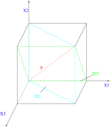
Figure 1: D3₅ (D3) and D3₄ (D3’) brane orientation wrt the fundamental cell of $T^{3}_{X}$ is shown. The red dashed line along which the two planes intersect indicate the unmagnetized direction.

The magnetized 4-plane $\Pi_{M}$ is spanned by the worldvolumes of the two D2-branes

$$D2_{4}^{\perp}=g_{4}(E_{x^{1}}-2q_{4}q_{5}E_{x^{2}}-2q_{5}E_{{\tilde{x}}^{3}})+h_{4}(E_{y^{3}}-q_{4}E_{{\tilde{y}}^{2}})=g_{4}\hat{E}_{g_{4}}+h_{4}\hat{E}_{h_{4}}$$ (18)

$$D2_{5}^{\perp}=g_{5}(E_{x^{1}}-5q_{4}q_{5}E_{x^{2}}+q_{5}E_{{\tilde{x}}^{3}})+h_{5}(E_{y^{3}}-q_{5}E_{{\tilde{y}}^{1}})=g_{5}\hat{E}_{g_{5}}+h_{5}\hat{E}_{h_{5}}$$ (19)

obtained neglecting the common longitudinal direction $P_{45}$ i.e. taking the orthogonal complements to $P_{45}$ of $D3_{4}$ and $D3_{5}$. The hypervolumes spanned by $\Pi_{M}$, $D2^{\perp}_{4}$, $D2^{\perp}_{5}$ are given by

$$\widehat{V}=\sqrt{\det(\hat{E}_{A}\cdot\hat{E}_{B})}$$ (20)

where $\hat{E}_{A}=\{\hat{E}_{g_{4}},\hat{E}_{h_{4}},\hat{E}_{g_{5}},\hat{E}_{h_{5}}\}$ for $\Pi_{M}$, while $\hat{E}_{a}=\{\hat{E}_{g_{4}},\hat{E}_{h_{4}}\}$ for $D2^{\perp}_{4}$ and $\hat{E}_{b}=\{\hat{E}_{g_{5}},\hat{E}_{h_{5}}\}$ for $D2^{\perp}_{5}$. The relevant scalar products are

$$|\hat{E}_{g_{4}}|^{2}=6\sqrt{2}\quad|\hat{E}_{h_{4}}|^{2}=2\sqrt{2}\quad|\hat{E}_{g_{5}}|^{2}=15\sqrt{2}\quad|\hat{E}_{h_{5}}|^{2}={5\over 4}\sqrt{2}$$ (21)

$$\hat{E}_{g_{4}}\cdot\hat{E}_{g_{5}}=6\sqrt{2}\quad\hat{E}_{h_{4}}\cdot\hat{E}_{h_{5}}=\sqrt{2}\quad\hat{E}_{g_{4}}\cdot\hat{E}_{h_{4}}=\hat{E}_{g_{4}}\cdot\hat{E}_{h_{5}}=\hat{E}_{g_{5}}\cdot\hat{E}_{h_{4}}=\hat{E}_{g_{5}}\cdot\hat{E}_{h_{5}}=0$$

So that

$$V(\Pi_{M})=18\quad A(D2^{\perp}_{4})=2\sqrt{6}\quad A(D2^{\perp}_{4})={5\over 2}\sqrt{6}$$ (22)

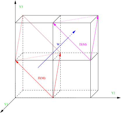
Figure 2: The projection of $D3_{4}$ and $D3_{5}$ brane on $T^{3}_{Y}$ leads two D1 branes, along the direction $\hat{E}_{h_{4}}$ and $\hat{E}_{h_{5}}$ indicated with red arrows. They span the magnetized plane $\Pi(M)$ orthogonal to the winding vector $W_{45}$ (blue arrows).

Then the intersection angles are such that

$$\prod_{I}\sin(\pi\epsilon^{I}_{ab})=V(\Pi_{M})/A(Dp_{a})A(Dp_{b})$$ (23)

In our 4-5 case, since $\sin(\pi\epsilon^{1}_{45})=\sin(\pi\epsilon^{2}_{45})$ for susy reasons, one has

$$\sin(\pi\epsilon_{45})=\sqrt{18/30}=\sqrt{3/5}$$ (24)

that means

$$\tan(\pi\epsilon_{45})=\sqrt{3/2}$$ (25)

that coincides with the result of diagonalizing $R_{45}$! In order to compute the index $I_{45}^{\perp}$ and confirm that the minimal winding is indeed $1/6$ it is very convenient to factorize the problem in the two subtori ${\bf T}^{6}={\bf T}^{3}_{X}{\bf T}^{3}_{Y}$. On the first subtorus ${\bf T}^{3}_{X}={\bf T}^{3}_{x^{1}x^{2}{\tilde{x}}^{3}}$, we have two D2-branes intersecting along the common direction $P_{45}$ at an angle such that $\cos(\beta^{X}_{ab})=\sqrt{2/5}$. The fig.(1) displays the the orientation of $P_{45}$ wrt the cell. As already stated $P_{45}$ winds only once within the fundamental cell. In the second sub-torus ${\bf T}^{3}_{X}={\bf T}^{3}_{{\tilde{y}}^{1}{\tilde{y}}^{2}y^{3}}$ the two D1-branes interesect only at the origin and span a plane orthogonal to $W_{45}$, as fig.(2) shows.

The distance between two such planes, i.e. intersections, along the direction of $W_{45}$ is $|W_{45}|/6$ hence $\nu_{min}=1/6$. Thus $I^{\perp}_{45}=1$, which is nicely consistent with open - closed channel duality after putting numbers $V(T^{6})=\sqrt{8}$, $\sin(\beta)=\sqrt{3/5}$, $\sqrt{\det(1+H_{4})}=2$ and $\sqrt{\det(1+H_{5})}=5/4$, $L_{P}=\sqrt{3\sqrt{2}}$ and $L_{P}^{\prime}=6/L_{W}=\sqrt{6/\sqrt{2}}$.

5 Gauge Coupling Thresholds

Once the perturbative open string spectrum is known, computing some of the low-energy effective couplings is quite straightforward. Tree level gauge couplings were determined in [16] and turned out to be given by

$${4\pi\over g_{a}^{2}}=e^{-\Phi}\sqrt{\det({\cal G}_{a}+{\cal F}_{a})}=e^{-\Phi}|W_{a}|\sqrt{\det({G}+{F}_{a})}$$ (1)

Moduli dependence is hidden inside the induced metric ${\cal G}_{a}$. The induced internal magnetic field ${\cal F}_{a}=F^{a}_{ij}\ \partial_{\alpha}X^{i}\partial_{\beta}X^{j}$ satisfies the standard Dirac quantization condition. At supersymmetric points, the expression simplifies and indeed coincides with the WZ term due to the identity of tension and charge for the magnetized brane (configuration). Moreover, in principle, for proper choices of the oblique magnetic fields all closed string moduli, except for the complexified dilaton, could be frozen. The ratios of the couplings would then be completely determined. More precisely, we are ignoring possible mixings of the open string Wilson line moduli, i.e. we are setting their VEV’s to zero for the time being.

Although a consistent variant of the AM model [15] has not yet been found, our aim is to extend the tree level analysis [mbt] to one-loop and derive the running of the gauge couplings as well as their threshold corrections. This is a preliminary step towards the study of gauge coupling unification in models with oblique magnetic fluxes or closely related (orbifold) models that might be phenomenologically more appealing but still solvable.

We will follow the strategy pioneered by [5, 59] and successfully applied to type I orbifolds in [23, 60], to generic type I vacuum configurations in [60] and to intersecting brane models in [62], based on the background field method.

As hinted at in the introduction, the method consists in applying an abelian, constant and small magnetic field in some spacetime directions, computing the effect of such an integrable deformation and then extracting the desired (quadratic) term in the one-loop effective action.

Only open strings that have at least one end on the spacetime magnetized brane will sense the presence of the magnetic field and can a priori contribute to the renormalization of the corresponding gauge coupling. In principle, one should consider dipole strings, preserving ${\cal N}=4$, as well as singly- and doubly-charged strings, preserving ${\cal N}=1$ or ${\cal N}=2$. However, similar to what happens in simpler cases with parallel magnetic fields or untwisted sector of orbifolds, ${\cal N}=4$ sectors neither contribute to the running nor to the thresholds, while ${\cal N}=1$ or ${\cal N}=2$ sectors contribute both to the running and to the thresholds. Massless open string states contribute to the logarithmic running, and we will retrieve the field-theory $\beta$-function coefficients studying the IR limit of the relevant one loop amplitudes. The contribution to the thresholds from ${\cal N}=2$ sectors is particularly simple since the gauge coupling is 1/2 BPS-saturated [63, 59, 23, 60], only the zero-modes coded in the ‘magnetically’ deformed internal lattice sum will survive but no string oscillator modes [64]. The contribution to the thresholds from ${\cal N}=1$ sectors is slightly more involved since the gauge coupling is not BPS-saturated in this case [23, 60]. As obvious from the discussion of the spectrum in Section 2 there are no lattice sums in these sectors, but magnetically shifted string oscillator modes can and do contribute. Luckily we will recast our anlysis along the lines of [62] where the modular integral for the case of intersecting branes were computed and finally expressed in terms of $\Gamma$ functions. Once again the moduli dependence hidden in the lattice sums or the magnetic shifts (T-dual to angles) can be fixed for particular choices of the internal oblique fluxes.

5.1 General analysis

For definiteness, we turn on an abelian magnetic field in spacetime directions 2 and 3, viz.

$$F_{\mu\nu}=\delta_{[\mu}^{2}\delta_{\nu]}^{3}fQ$$ (2)

where $Q$ is one of the generator of the unbroken CP group, normalized so that $Tr_{N}(Q)=0$ and $Tr_{N}(Q^{2})=1/2$. Depending on the embedding of $Q$ in the CP group one can find different behaviours. We will mostly focus on the case in which $Q$ is a generator of a non-abelian and thus non-anomalous factor.

As for internal fluxes, the spacetime magnetic deformation is integrable. Amplitudes on surfaces with no boundaries, such as torus and the Klein Bottle are insensible to the external field. Annulus and Möbius strip do couple to the external field and the connected generating functional depends on $f$. The main effects of turning on $f$ are the magnetic shifts $\epsilon^{Q}_{ab}$ of the transverse spacetime modes and the degeneracy $I^{Q}_{ab}$ of Landau levels for the string modes in the $[23]$ plane. Both are related to the charge $Q$ of the open string according to

$$\epsilon^{Q}_{ab}={1\over\pi}[\arctan(Q_{a}f)+\arctan(Q_{b}f)]$$ (3)

for ${\cal A}_{ab}(f)$ with $I^{Q}_{ab}=(Q_{a}+Q_{b})f/2\pi$, and

$$\epsilon^{Q}_{aa}={2\over\pi}\arctan(Q_{a}f)$$ (4)

for ${\cal M}_{aa}(f)$ with $\hat{I}^{Q}_{aa}=2Q_{a}f/2\pi$.

Expanding the Annulus and the Möbius amplitudes up to second order in $f$ one gets the one-loop gauge threshold for the group $Q$ belongs to [23, 59]

$$\Delta_{Q}=\int\frac{dt}{t}({\cal A}_{Q}^{\prime\prime}(0)+{\cal M}_{Q}^{\prime\prime}(0))=\int\frac{dt}{4t}B_{Q}(t)$$ (5)

that implicitly depends on the moduli fields through the dependence on the latter of the masses of the unoriented open string states running in the loop. We use $Q$ to label the (factor) group we are computing the threshold of.

The only allowed momenta are along the light-cone directions $0$ and $1$. Analytic continuation and volume regularization thus yield

$$\int{V_{LC}dp^{+}dp^{-}\over(2\pi)^{2}}\exp(-\pi{\alpha^{\prime}}tp^{+}p^{-})={V_{LC}\over(2\pi)^{2}{\alpha^{\prime}}t}\quad.$$ (6)

One can easily write down the contribution of singly as well as doubly charged unoriented strings:

$${\cal A}^{{\cal N}=1}_{Q}(f) = \sum_{a,b}I_{ab}\sum_{\alpha,\beta}{c_{\alpha\beta}\over 2}tr_{N_{a}\times N_{b}}\left[{(Q_{a}+Q_{b})f\over(2\pi)^{3}{\alpha^{\prime}}t}{\theta\left[{}^{\alpha}_{\beta}\right](\epsilon_{ab}^{Q}\tau_{A}|\tau_{A})\over\theta_{1}(\epsilon_{ab}^{Q}\tau_{A}|\tau_{A})}\right]\prod_{I}{\theta\left[{}^{\alpha}_{\beta}\right](\epsilon^{I}_{ab}\tau_{A}|\tau_{A})\over\theta_{1}(\epsilon^{I}_{ab}\tau_{A}|\tau_{A})}$$

$${\cal M}^{{\cal N}=1}_{Q}(f) = -\sum_{a}\hat{I}_{aa}\sum_{\alpha\beta}c_{\alpha\beta}\;Tr_{N_{a}}\left[\frac{Q_{a}f}{(2\pi)^{3}\alpha t}\frac{\theta[^{\alpha}_{\beta}](\epsilon^{Q}_{aa}\tau_{A}|\tau_{M})}{\theta_{1}(\epsilon^{Q}_{aa}\tau_{A}|\tau_{M})}\right]\prod_{I}\frac{\theta[^{\alpha}_{\beta}](\epsilon^{I}_{aa}\tau_{A}|\tau_{M})}{\theta_{1}(\epsilon^{I}_{aa}\tau_{A}|\tau_{M})})$$ (7)

where $\tau_{A}=it/2$, $\tau_{M}=\tau_{A}+1/2$, and, denoting as usual by $u$ the internal unmagnetized direction, when present,

$$\quad{\cal A}^{{\cal N}=2}_{Q}(f) = -i\sum_{a,b}\ I^{\perp}_{ab}\Lambda^{u}_{ab}(\tau_{A})\sum_{\alpha,\beta}{c_{\alpha\beta}\over 2}tr_{N_{a}\times N_{b}}\left[{(Q_{a}+Q_{b})f\over(2\pi)^{3}{\alpha^{\prime}}t}{\theta\left[{}^{\alpha}_{\beta}\right](\epsilon_{ab}^{Q}\tau_{A}|\tau_{A})\over\theta_{1}(\epsilon_{ab}^{Q}\tau_{A}|\tau_{A})}\right]$$ (8)

$${\theta\left[{}^{\alpha}_{\beta}\right](0|\tau_{A})\over\eta^{3}(\tau_{A})}\prod_{I\neq u}{\theta\left[{}^{\alpha}_{\beta}\right](\epsilon^{I}_{ab}\tau_{A}|\tau_{A})\over\theta_{1}(\epsilon^{I}_{ab}\tau_{A}|\tau_{A})}$$

$${\cal M}^{{\cal N}=2}_{Q}(f) = i\sum_{a}\hat{I}_{aa}^{\perp}\Lambda^{u}_{aa}(\tau_{A})\sum_{\alpha\beta}c_{\alpha\beta}N_{a}Tr_{N_{a}}\left[\frac{Q_{a}f}{(2\pi)^{3}\alpha t}\frac{\theta[^{\alpha}_{\beta}](\epsilon^{Q}_{aa}\tau_{A}|\tau_{M})}{\theta_{1}(\epsilon^{Q}_{aa}\tau_{A}|\tau_{M})}\right]\frac{\theta[^{\alpha}_{\beta}](0|\tau_{M})}{\eta^{3}(\tau_{M})}$$ (9)

$$\prod_{I\neq u}\frac{\theta[^{\alpha}_{\beta}](\epsilon^{I}_{aa}\tau_{A}|\tau_{M})}{\theta_{1}(\epsilon^{I}_{aa}\tau_{A}|\tau_{M})}$$

${\cal N}=4$ sectors, such as neutral and dipole strings with opposite $Q$ charge at their ends do not contribute to the thresholds since their modes are not shifted and they simply receive an overall factor reflecting the ’magnetic deformation’ of the lattice sum. Similarly, the Möbius strip does not contribute if $Q$ is part of $SO(N_{0})$, associated to ‘unmagnetized’ branes if present, so that the two ends have opposite charge. Henceforth we set ${\alpha^{\prime}}=1/2$ for convenience.

5.2 ${\cal N}=1$ sectors

In ${\cal N}=1$ supersymmetric sectors, expanding to quadratic order one gets

$${\cal A}^{{\cal N}=1}_{Q}(f) = i\sum_{a,b}\ I_{ab}\frac{1}{2}\left(\frac{f}{2\pi}\right)^{2}\sum_{\alpha\beta}\frac{c_{\alpha\beta}}{{8\pi^{2}}}\;Tr_{N_{a}\times N_{b}}(Q_{a}+Q_{b})^{2}\frac{\theta^{\prime\prime}[^{\alpha}_{\beta}](0)}{\eta^{3}}\prod_{I}\frac{\theta[^{\alpha}_{\beta}](\epsilon^{I}_{ab}\tau_{A}|\tau_{A})}{\theta_{1}(\epsilon^{I}_{ab}\tau_{A}|\tau_{A})})+...$$

$${\cal M}^{{\cal N}=1}_{Q}(f) = -i\sum_{a}\ I_{aa}\frac{1}{2}\left(\frac{f}{2\pi}\right)^{2}\sum_{\alpha\beta}\frac{c_{\alpha\beta}}{2\pi^{2}}\;Tr_{N_{a}}(Q_{a}^{2})\frac{\theta^{\prime\prime}[^{\alpha}_{\beta}](0|\tau_{M})}{\eta^{3}(\tau_{M})}\prod_{I}\frac{\theta[^{\alpha}_{\beta}](\epsilon^{I}_{aa}\tau_{A}|\tau_{M})}{\theta_{1}(\epsilon^{I}_{aa}\tau_{A}|\tau_{M})}+...$$ (10)

Summing over spin structures and using the generalized Jacobi $\theta$ function identity

$$\sum_{\alpha\beta}c_{\alpha\beta}\frac{\theta^{\prime\prime}[^{\alpha}_{\beta}](0)}{\eta^{3}}\prod_{I}\frac{\theta[^{\alpha}_{\beta}](\epsilon^{I}\tau)}{\theta_{1}(\epsilon^{I}\tau)}=2\pi\sum_{I}\frac{\theta_{1}^{\prime}(\epsilon^{I}_{ab}\tau)}{\theta_{1}(\epsilon^{I}\tau)}$$ (11)

give

$$B_{Q}^{{\cal N}=1}(t) = \frac{i}{\pi}\sum_{a,b}I_{ab}Tr_{N_{a}\times N_{b}}(Q_{a}+Q_{b})^{2}\sum_{I}\frac{\theta_{1}^{\prime}(\epsilon^{I}_{ab}\tau_{A}|\tau_{A})}{\theta_{1}(\epsilon^{I}_{ab}\tau_{A}|\tau_{A})}$$

$$\hat{B}_{Q}^{{\cal N}=1}(t) = -\frac{i}{\pi}\sum_{a}I_{aa}Tr_{N_{a}}(2Q_{a}^{2})\sum_{I}\frac{\theta_{1}^{\prime}(\epsilon^{I}_{aa}\tau_{A}|\tau_{M})}{\theta_{1}(\epsilon^{I}_{aa}\tau_{A}|\tau_{M})}$$ (12)

At this point it is easy to extract the $\beta$-function coefficents from the IR limit of (5.2)

$$b_{Q}^{{\cal N}=1} = \frac{1}{2}\sum_{a,b}I_{ab}Tr_{N_{a}\times N_{b}}(Q_{a}+Q_{b})^{2}$$

$$\hat{b}_{Q}^{{\cal N}=1} = -\frac{1}{2}\sum_{a}I_{aa}Tr_{N_{a}}(2Q_{a})^{2}$$ (13)

Since all vectors belong to ${\cal N}=4$ multiplets, $\beta$-function are positive, i.e. all non-abelian couplings grow in the UV.

In order to perform the integral and compute $\Delta_{Q}$ we switch to the transverse channel and end up with the following expressions

$$\Delta_{Q}^{{\cal N}=1} = \frac{1}{\pi}\sum_{a,b}I_{ab}Tr_{N_{a}\times N_{b}}(Q_{a}+Q_{b})^{2}\sum_{I}\int_{0}^{\infty}\frac{\theta_{1}^{\prime}(\epsilon^{I}_{ab}|i\ell)}{\theta_{1}(\epsilon^{I}_{ab}|i\ell)}\;d\ell$$

$$\hat{\Delta}_{Q}^{{\cal N}=1} = -\frac{1}{2\pi}\sum_{a}Tr_{N_{a}}(2Q_{a})^{2}I_{aa}\sum_{I}\int_{0}^{\infty}\frac{\theta_{1}^{\prime}(\epsilon^{I}_{0a}|i\ell+1/2)}{\theta_{1}(\epsilon^{I}_{0a}|i\ell+1/2)}\;d\ell$$ (14)

Series expansion

$$\frac{{\theta_{1}^{\prime}(\epsilon|\tau)}}{\theta_{1}(\epsilon|\tau)}=\pi\cot(\pi\epsilon)+2\sum_{k=1}^{\infty}\zeta(2k)\epsilon^{k}(E_{2k}(\tau)-1)\quad,$$ (15)

where $\zeta(2k)=(2\pi)^{2k}|B_{2k}|/(2k)!$ and $E_{2k}(\tau)$ is an Eisenstein series with modular weight $2k$, expose the potentially divergent terms

$$\delta_{Q}^{{\cal N}=1} = \sum_{a,b}\frac{I_{ab}}{4}Tr_{N_{a}\times N_{b}}(Q_{a}+Q_{b})^{2}\sum_{I}\cot(\pi\epsilon^{I}_{ab})\int_{0}^{\infty}d\ell$$

$$\hat{\delta}_{Q}^{{\cal N}=1} = -2\sum_{a}\hat{I}_{aa}Tr_{N_{a}}(Q_{a}^{2})\sum_{I}\cot(\pi\epsilon^{I}_{0a})\int_{0}^{\infty}d\ell$$ (16)

that eventually cancel thanks to (NS-NS) tadpole cancellation, for the non-anomalous $Q$, with $Tr(Q)=0$. The latter condition has to be used in order to dispose of the divergent terms with $f$ insertions in two different boundaries. Divergences from insertions on the same boundary cancel between annulus and Möbius strip thanks to tadpole cancellation.

The finite terms boil down to integrals of the form [62]

$$\int_{0}^{\infty}d\ell\sum_{k=1}^{\infty}2\zeta(2k)\epsilon^{k}(E_{2k}(i\ell)-1)=-\pi\log\left[\Gamma(1-\epsilon)\over\Gamma(1+\epsilon)\right]+2\pi\epsilon\gamma_{E}$$ (17)

$$\int_{0}^{\infty}d\ell\sum_{k}2\zeta(2k)\epsilon^{k}(E_{2k}(i\ell+1/2)-1)=-\pi\log\left[\Gamma(1-2\epsilon)\over\Gamma(1+2\epsilon)\right]+2\pi\epsilon\gamma_{E}$$ (18)

Actually the last contributions, linear in $\epsilon$, drop after summing over the three internal directions in supersymmetric cases.

Summing the various contributions one finally gets

$$\Delta^{{\cal N}=1}_{Q} = -\sum_{a,b}\frac{I_{ab}}{2}Tr_{N_{a}\times N_{b}}(Q_{a}^{2}+Q_{b}^{2})\sum_{I}\log\left[\Gamma(1-\epsilon^{I}_{ab})\over\Gamma(1+\epsilon^{I}_{ab})\right]$$

$$\hat{\Delta}^{{\cal N}=1}_{Q} = \sum_{a}I_{aa}Tr_{N_{a}}(2Q_{a})^{2}\sum_{I}\log\left[\Gamma(1-\epsilon^{I}_{aa})\over\Gamma(1+\epsilon^{I}_{aa})\right]\quad,$$ (19)

where $\epsilon^{I}_{aa}=2\epsilon^{I}_{ao}$.

5.3 ${\cal N}=2$ sectors

Thresholds corrections from ${\cal N}=2$ sectors are much easier to compute since they correspond to BPS saturated couplings. Indeed, for ${\cal N}=2$ supersymmetric sectors, the terms quadratic in $f$ read

$${\cal A}^{{\cal N}=2}_{Q}(f) = \sum_{a,b}I_{ab}^{\perp}\Lambda^{u}_{ab}(\tau_{A})\frac{1}{2}\left(\frac{f}{2\pi}\right)^{2}\sum_{\alpha\beta}\frac{c_{\alpha\beta}}{8\pi^{2}}\;Tr_{N_{a}\times N_{b}}(Q_{a}+Q_{b})^{2}\frac{\theta^{\prime\prime}[^{\alpha}_{\beta}](0|\tau_{A})}{\eta^{3}(\tau_{A})}\frac{\theta[^{\alpha}_{\beta}](0|\tau_{A})}{\eta^{3}(\tau_{A})}$$

$$\prod_{I\neq u}\frac{\theta[^{\alpha}_{\beta}](\epsilon^{I}_{ab}\tau_{A}|\tau_{A})}{\theta_{1}(\epsilon^{I}_{ab}\tau_{A}|\tau_{A})}+...$$

$${\cal M}^{{\cal N}=2}_{Q}(f) = \sum_{a}I_{aa}^{\perp}\Lambda^{u}_{aa}(\tau_{A})\frac{1}{2}\left(\frac{f}{2\pi}\right)^{2}\sum_{\alpha\beta}{c_{\alpha\beta}\over 8\pi^{2}}\;Tr_{N_{a}}(2Q_{a})^{2}\frac{\theta^{\prime\prime}[^{\alpha}_{\beta}](0|\tau_{M})}{\eta^{3}(\tau_{M})}$$ (20)

$$\frac{\theta[^{\alpha}_{\beta}](0|\tau_{M})}{\eta^{3}(\tau_{M})}\prod_{I\neq u}\frac{\theta[^{\alpha}_{\beta}](\epsilon^{I}_{aa}\tau_{A}|\tau_{M})}{\theta_{1}(\epsilon^{I}_{aa}\tau_{A}|\tau_{M})})+...$$

and the Jacobi $\theta$ function identity

$$\sum_{\alpha\beta}c_{\alpha\beta}\frac{\theta^{\prime\prime}[^{\alpha}_{\beta}](0)}{\eta^{3}}\frac{\theta[^{\alpha}_{\beta}](0)}{\eta^{3}}\prod_{I\neq u}\frac{\theta[^{\alpha}_{\beta}](\zeta^{I}|\tau)}{\theta_{1}(\zeta^{I}|\tau)}=4\pi^{2}\quad,$$ (21)

valid for $\sum_{I}\zeta^{I}=0$, imply that only the lattice sum over 1/2 BPS states contributes.

Manipulations similar to the above yield the following results for $\beta$-function coefficents in ${\cal N}=2$ sectors,

$$b_{Q}^{{\cal N}=2} = \sum_{a,b}I_{ab}^{\perp}Tr_{N_{a}\times N_{b}}(Q_{a}+Q_{b})^{2}$$

$$\hat{b}_{Q}^{{\cal N}=2} = -\sum_{a}\hat{I}_{aa}^{\perp}N_{a}Tr_{N_{a}}(2Q_{a})^{2}$$ (22)

Since all vectors belong to ${\cal N}=4$ multiplets, $\beta$-functions are positive, i.e. all non-abelian couplings grow in the UV.

For the thresholds one has

$$\Delta_{Q}^{{\cal N}=2} = \frac{1}{2}\sum_{a,b}I_{ab}^{\perp}Tr_{N_{a}\times N_{b}}(Q_{a}+Q_{b})^{2}\int_{0}^{\infty}\Lambda_{ab}^{u}(it)\;\frac{dt}{t}$$

$$\Delta_{Q}^{{\cal N}=2} = -\frac{1}{2}\sum_{a}I_{aa}^{\perp}Tr_{N_{a}}(2Q_{a})^{2}\int_{0}^{\infty}\Lambda_{aa}^{u}(it)\;\frac{dt}{t}$$ (23)

The integrals of the ‘regulated’ lattice sums can be performed with the aid of the formula

$$\int_{0}^{\infty}\frac{dt}{t}\sum_{(k_{1},k_{2})\neq(0,0)}\exp(-\pi{\ell}|k_{1}+Uk_{2}|^{2}/V_{2}U_{2})=\gamma_{E}-\log[4\pi V_{2}U_{2}|\eta(U)|^{4}]$$ (24)

where $V_{2}$ is the volume and $U$ the complex structure of the unmagnetized torus. Inserting into (24) one gets

$$\Delta_{Q}^{{\cal N}=2} = \frac{1}{2}\sum_{a,b}I_{ab}^{\perp}Tr_{N_{a}\times N_{b}}(Q_{a}+Q_{b})^{2}[\ln(V_{2}U_{2}|\eta(U)|^{4}4\pi)-\gamma_{E}]$$

$$\Delta_{Q}^{{\cal N}=2} = -2\sum_{a}I_{aa}^{\perp}Tr_{N_{a}}(Q_{a}^{2})[\ln(4V_{2}U_{2}|\eta(U)|^{4}4\pi)-\gamma_{E}]$$ (25)

For proper choices of the internal oblique fluxes all closed string moduli are fixed, modulo mixing with massless open string states, and the above formulae give simply numbers as we will momentarily see.

We would now like to comment on the effect of large extra dimensions on the coupling costants running. Setting $U_{1}=0$ for simplicity and expanding the logarithm in the last expression yields

$$\ln(4\pi V_{2}U_{2}|\eta(U)|^{4})=\ln(4\pi VU_{2})-\frac{\pi r_{2}}{3r_{1}}+4\sum_{n}\ln(1-e^{-2\pi\frac{r_{2}}{r_{1}}n})$$ (26)

where $r_{2}\,r_{1}$ are the radii of $T^{2}_{u}$ so that $U_{2}=r_{2}/r_{1}$. One can envisage two different situations

• $r_{2}\sim r_{1}$, when the radii are fixed at the string scale, and corrections do not seem to affect the usual logarithmic behavior.

• $r_{2}>>r_{1}$. Power corrections are dominant, this is the scenario already described in [65], where power corrections are induced by the running in the loop of bulk particle, with KK towers organized in ${\cal N}=2$ multiplets. Power law behavior can be exploited to lower the unification scale. This is achieved if one of the unmagnetized eigenvectors points toward a large extra dimension.

6 Outlook

In the present paper we have derived explicit formulae for the one-loop contributions to type I string compactifications on tori with arbitrary magnetic fluxes [15, 55, 16]. We have checked consistency with the transverse channel and identified the correct tadpole conditions. Further insights in the geometry of these vacuum configurations has been gained by means of T-duality [40, 41]. We have then turned our attention to the one-loop threshold corrections to the non-abelian gauge couplings and derived very compact expressions thereof, relying on similar analyses for type I orbifolds [23, 60] and intersecting brane models [62]. Although unrealistic in many respects, toroidal models of this kind may be used as building blocks or rather starting points for type I orbifolds and other solvable (supersymmetric) compactifications. In particular the emergence of induced lower dimensional R-R charges and NS-NS tensions of both signs plays a crucial role in solving [53, 37] some long standing puzzles [66].

Given the high level of control one has on this class of models, one can restrict one’s attention onto those that resemble as closely as possible the Standard Model or some of its supersymmetric or grand unified generalizations. In principle, the magnetic fields can be tuned so as to produce the desired gauge group and fermionic content, and achieve gauge coupling unification. With more effort one can try to generate the correct pattern of Yukawa couplings and trigger supersymmetry breaking in a controllable way [67].

Stabilizing dilaton and axion may require switching to a T-dual description in terms of D3-branes that allows the introduction of closed string 3-form fluxes. Yet the same goal may be achieved by means of non-perturbative effects such as D5-brane and D-string instantons. In any case, at present the possibility that all moduli be stabilized by perturbative effects remains a challenge. The presence of dilaton tadpoles at different orders in perturbation theory may help achieving this goal.

Moreover, open string Wilson line moduli, especially those charged under the anomalous $U(1)$’s, can mix with closed string moduli, due to their contribution to D-terms. This complicates the analysis, that has been so far performed at the origin of the open string moduli space. In this respect, it is reassuring to observe that scalars in vector multiplets can be lifted by orbifold projections and in any case they can be treated exactly along the lines of [19]. In order to set the stage for the discussion of the lifting of scalars in chiral multiplets one should compute the superpotential, i.e. the Yukawa couplings [68]. For charged open string states, the relevant amplitudes involve mutually non-abelian twists in general and the perspective of computing them is daunting. Yet it may be worth proving.

Appendix A: Some useful formulae

$$\prod_{I\neq u}\sin(\pi\epsilon^{I}_{ab}) = \prod_{I\neq u}{1\over 2i}(e^{i\pi\epsilon^{I}_{ab}}-e^{-i\pi\epsilon^{I}_{ab}})$$ (1)

$$= \sqrt{\prod_{I\neq u}e^{-i\pi\epsilon^{I}_{ab}}\left({1\over 2i}\right)(e^{i2\pi\epsilon^{I}_{ab}}-1)e^{i\pi\epsilon^{I}_{ab}}\left(-{1\over 2i}\right)(e^{-i2\pi\epsilon^{I}_{ab}}-1)}$$

$$= \sqrt{\det^{\prime}\left({R_{ab}-1\over 2}\right)}={\sqrt{\det^{\prime}(H_{a}+H_{b})}\over\sqrt{\det(1+H_{a})}\sqrt{\det(1+H_{b})}}$$

$$\prod_{I\neq u}\cos(\pi\epsilon^{I}_{ab}) = \prod_{I\neq u}{1\over 2}(e^{i\pi\epsilon^{I}_{ab}}+e^{-i\pi\epsilon^{I}_{ab}})$$ (2)

$$= \sqrt{\prod_{I\neq u}e^{-i\pi\epsilon^{I}_{ab}}\left({1\over 2}\right)(e^{i2\pi\epsilon^{I}_{ab}}+1)e^{i\pi\epsilon^{I}_{ab}}\left({1\over 2}\right)(e^{-i2\pi\epsilon^{I}_{ab}}+1)}$$

$$= \sqrt{\det\left({R_{ab}+1\over 2}\right)}={\sqrt{\det(1+H_{a}H_{b})}\over\sqrt{\det(1+H_{a})}\sqrt{\det(1+H_{b})}}$$

$$= Tr(U_{ab})=Tr(U_{a}U_{b})$$

where $U_{a}={{\rm AExp}(-{1\over 2}F_{a,ij}\Gamma^{ij})\over\sqrt{\det(1+H_{a})}}$. As a corollary

$$\prod_{I\neq u}2\cos(\pi\epsilon^{I}_{a})={1\over\sqrt{\det(1+H_{a})}}=Tr_{s}(U_{a})$$ (3)

$$2\sum_{I\neq u}\cos(2\pi\epsilon^{I}_{ab})=\sum_{I\neq u}(e^{2i\pi\epsilon^{I}_{ab}}+e^{-2i\pi\epsilon^{I}_{ab}})=Tr_{v}(R_{ab})=Tr_{v}(R_{a}R_{b})$$ (4)

Appendix B: Theta functions

Definitions

In order to fix notations, we report in this appendix the Jacobi $\theta$-functions, we used throughout the paper. Let $q=e^{2\pi i\tau}\,$ they are defined as guassian sums

$$\theta\left[{}^{\alpha}_{\beta}\right](z|\tau)=\sum_{n}q^{{1\over 2}(n-\alpha)^{2}}e^{2\pi i(z-\beta)(n-\alpha)}$$ (5)

where $\alpha\ \beta\in R$.
Equivalently, for particular values of characteristics, such as $\,\alpha\;\beta=0\mbox{ , }\frac{1}{2}\;$ they are given also in terms of infinite product as follows

$$\theta\left[{}^{\frac{1}{2}}_{\frac{1}{2}}\right](z|\tau)=\theta_{1}(z|\tau) = 2q^{1\over 8}\sin(\pi z)\prod_{m=1}^{\infty}(1-q^{m})(1-e^{2\pi iz}q^{m})(1-e^{-2\pi iz}q^{m})$$

$$\theta\left[{}^{\frac{1}{2}}_{0}\right](z|\tau)=\theta_{2}(z|\tau) = 2q^{1\over 8}\cos(\pi z)\prod_{m=1}^{\infty}(1-q^{m})(1+e^{2\pi iz}q^{m})(1+e^{-2\pi iz}q^{m})$$

$$\theta\left[{}^{0}_{0}\right](z|\tau)=\theta_{3}(z|\tau) = \prod_{m=1}^{\infty}(1-q^{m})(1+e^{2\pi iz}q^{m-\frac{1}{2}})(1+e^{-2\pi iz}q^{m-\frac{1}{2}})$$

$$\theta\left[{}^{0}_{\frac{1}{2}}\right](z|\tau)=\theta_{4}(z|\tau) = \prod_{m=1}^{\infty}(1-q^{m})(1-e^{2\pi iz}q^{m-\frac{1}{2}})(1-e^{-2\pi iz}q^{m-\frac{1}{2}})$$ (6)

The Dedekind function $\eta$ is defined as

$$\eta(\tau)=q^{1\over 24}\prod_{n=1}^{\infty}(1-q^{n})$$ (7)

The Eisenstein series are

$$E_{r}=\sum_{m\neq 0}^{\infty}\sum_{n\neq 0}^{\infty}\frac{1}{(m+n\tau)^{r}}$$ (8)

with $r>2$. Moreover they can be expressed as polynomial of elliptic funtions

$$E_{2k}(\tau)=1+{(2\pi i)^{2k}\over(2k-1)!\zeta(2k)}\sum_{n=1}^{\infty}\sigma_{2k-1}(n)e^{2\pi in\tau}$$ (9)

where $\zeta(2k)$ is Riemann zeta function and $\sigma_{2k-1}(n)$ is the divisor function

$$\sigma_{2k-1}(n)=\sum_{d|n}d^{2k-1}\quad.$$ (10)

Modular Transformations

Under T and S modular trasformations on the arguments the functions, given above, have pecular properties:

$$\theta\left[{}^{\alpha}_{\beta}\right](z|\tau+1) = e^{-i\pi\alpha(\alpha-1)}\ \theta\left[{}^{\alpha}_{\beta+\alpha-\frac{1}{2}}\right](z|\tau)$$

$$\eta(\tau+1) = e^{{i\pi\over 12}}\,\eta(\tau)$$

$$E_{2k}(\tau+1) = E_{2k}(\tau)$$

$$\theta\left[{}^{\alpha}_{\beta}\right](\frac{z}{\tau}|-{1\over\tau}) = (-i\tau)^{1\over 2}\,e^{2i\pi\alpha\beta+i\pi z^{2}/\tau}\ \theta\left[{}^{\beta}_{-\alpha}\right](z|\tau)$$

$$\eta(-{1\over\tau}) = (-i\tau)^{1\over 2}\,\eta(\tau)$$

$$E_{2k}(-{1\over\tau}) = \tau^{2}kE_{2k}(\tau)$$ (11)

The modular transformation P on the Jacobi functions is more involved as it consists in a sequence of T and S transformation ($P=TST^{2}S$). on the modular parameter $\tau_{M}=\frac{1}{2}+\frac{it}{2}$

$$\theta\left[{}^{\alpha}_{\beta}\right]({z\over it}|\frac{1}{2}+\frac{i}{2t}) = e^{-i\pi\alpha(\alpha-1)-2\pi i(\alpha+\beta-1/2)^{2}+2\pi z^{2}/t}\,\sqrt{-it}\;\theta\left[{}^{\alpha+2\beta-2}_{1/2-\alpha-\beta}\right](z|\frac{1}{2}+\frac{it}{2})$$

$$\eta(\frac{1}{2}+\frac{i}{2t}) = e^{i\pi/4}\sqrt{-it}\;\eta(\frac{1}{2}+\frac{it}{2})$$ (12)

References

• [1] E. S. Fradkin and A. A. Tseytlin, Phys. Lett. B 158 (1985) 316;
• [2] A. Abouelsaood, C. G. . Callan, C. R. Nappi and S. A. Yost, Nucl. Phys. B 280 (1987) 599.
• [3] C. G. . Callan, C. Lovelace, C. R. Nappi and S. A. Yost, Nucl. Phys. B 308, 221 (1988).
• [4] V. V. Nesterenko, Int. J. Mod. Phys. A 4 (1989) 2627.
• [5] C. Bachas and M. Porrati, Phys. Lett. B 296, 77 (1992) [arXiv:hep-th/9209032].
• [6] C. Bachas, arXiv:hep-th/9503030.
• [7] For review see e.g. Class. Quant. Grav.  17 (2000) R41 [arXiv:hep-ph/0006190]. E. Kiritsis, Fortsch. Phys.  52, 200 (2004) [arXiv:hep-th/0310001]. C. Kokorelis, arXiv:hep-th/0402087. A. M. Uranga, Class. Quant. Grav.  20, S373 (2003) [arXiv:hep-th/0301032]. R. Blumenhagen, M. Cvetic, P. Langacker and G. Shiu, arXiv:hep-th/0502005.
• [8] J. Dai, R. G. Leigh and J. Polchinski, Mod. Phys. Lett. A 4, 2073 (1989). R. G. Leigh, Mod. Phys. Lett. A 4, 2767 (1989).
• [9] J. F. Morales, C. A. Scrucca and M. Serone, Nucl. Phys. B 552, 291 (1999) [arXiv:hep-th/9812071]. C. A. Scrucca and M. Serone, Nucl. Phys. B 556, 197 (1999) [arXiv:hep-th/9903145].
• [10] M. Bianchi and Y. S. Stanev, Nucl. Phys. B 523 (1998) 193 [arXiv:hep-th/9711069].
• [11] I. Antoniadis, E. Dudas and A. Sagnotti, Nucl. Phys. B 544 (1999) 469 [hep-th/9807011];
• [12] I. Antoniadis, G. D’Appollonio, E. Dudas and A. Sagnotti, Nucl. Phys. B 553 (1999) 133 [hep-th/9812118];
• [13] C. Angelantonj and A. Sagnotti, Phys. Rept.  371 (2002) 1 [arXiv:hep-th/0204089].
• [14] M. Larosa, arXiv:hep-th/0111187, arXiv:hep-th/0212109; G. Pradisi, arXiv:hep-th/0210088. M. Larosa and G. Pradisi, Nucl. Phys. B 667, 261 (2003) [arXiv:hep-th/0305224].
• [15] I. Antoniadis and T. Maillard, arXiv:hep-th/0412008.
• [16] M. Bianchi and E. Trevigne, arXiv:hep-th/0502147.
• [17] L. E. Ibanez, R. Rabadan and A. M. Uranga, Nucl. Phys. B 542 (1999) 112 [arXiv:hep-th/9808139]. G. Aldazabal, D. Badagnani, L. E. Ibanez and A. M. Uranga, JHEP 9906 (1999) 031 [arXiv:hep-th/9904071]. E. Kiritsis and P. Anastasopoulos, JHEP 0205, 054 (2002) [arXiv:hep-ph/0201295].
• [18] P. Anastasopoulos, JHEP 0308, 005 (2003) [arXiv:hep-th/0306042].
• [19] M. Bianchi, G. Pradisi and A. Sagnotti, Nucl. Phys. B 376 (1992) 365;
• [20] M. Bianchi, Nucl. Phys. B 528 (1998) 73 [arXiv:hep-th/9711201];
• [21] E. Witten, JHEP 9802 (1998) 006 [arXiv:hep-th/9712028].
• [22] P. Di Vecchia and A. Liccardo, NATO Adv. Study Inst. Ser. C. Math. Phys. Sci.  556, 1 (2000) [arXiv:hep-th/9912161]. P. Di Vecchia and A. Liccardo, arXiv:hep-th/9912275.
• [23] I. Antoniadis, C. Bachas and E. Dudas, Nucl. Phys. B 560, 93 (1999) [arXiv:hep-th/9906039].
• [24] See e.g. R. Blumenhagen, Fortsch. Phys.  53, 426 (2005) [arXiv:hep-th/0412025].
• [25] P. Anastasopoulos and A. B. Hammou, arXiv:hep-th/0503061. P. Anastasopoulos, arXiv:hep-th/0503055. P. Anastasopoulos and A. B. Hammou, arXiv:hep-th/0503044.
• [26] S. Kachru, M. B. Schulz and S. Trivedi, JHEP 0310, 007 (2003) [arXiv:hep-th/0201028]. arXiv:hep-th/0303016; J. F. Cascales and A. M. Uranga, arXiv:hep-th/0303024.
• [27] J. P. Derendinger, C. Kounnas, P. M. Petropoulos and F. Zwirner, arXiv:hep-th/0503229. R. Blumenhagen, M. Cvetic, F. Marchesano and G. Shiu, JHEP 0503, 050 (2005) [arXiv:hep-th/0502095]. D. E. Diaconescu, E. Dell’Aquila and G. Pradisi, to appear soon.
• [28] N. Kaloper and R. C. Myers, JHEP 9905, 010 (1999) [arXiv:hep-th/9901045]. C. Angelantonj, S. Ferrara and M. Trigiante, JHEP 0310 (2003) 015 [arXiv:hep-th/0306185]. C. Angelantonj, S. Ferrara and M. Trigiante, Phys. Lett. B 582 (2004) 263 [arXiv:hep-th/0310136]. G. Dall’Agata and S. Ferrara, arXiv:hep-th/0502066. G. Dall’Agata, R. D’Auria and S. Ferrara, arXiv:hep-th/0503122. G. Villadoro and F. Zwirner, arXiv:hep-th/0503169.
• [29] A. Sagnotti, arXiv:hep-th/0208020.
• [30] G. Pradisi and A. Sagnotti, Phys. Lett. B 216, 59 (1989).
• [31] M. Bianchi and A. Sagnotti, Nucl. Phys. B 361, 519 (1991). M. Bianchi and A. Sagnotti, Phys. Lett. B 247, 517 (1990).
• [32] Z. Kakushadze, G. Shiu and S. H. Tye, Phys. Rev. D 58 (1998) 086001 [arXiv:hep-th/9803141];
• [33] C. Angelantonj, Nucl. Phys. B 566 (2000) 126 [arXiv:hep-th/9908064].
• [34] G. Pradisi, arXiv:hep-th/0310154.
• [35] S. Sugimoto, Prog. Theor. Phys.  102 (1999) 685 [arXiv:hep-th/9905159].
• [36] E. Dudas, J. Mourad and A. Sagnotti, Nucl. Phys. B 620, 109 (2002) [arXiv:hep-th/0107081].
• [37] E. Dudas and C. Timirgaziu, arXiv:hep-th/0502085.
• [38] M. Bianchi, J. F. Morales and G. Pradisi, Nucl. Phys. B 573 (2000) 314 [arXiv:hep-th/9910228].
• [39] C. Angelantonj, M. Cardella and N. Irges, arXiv:hep-th/0503179.
• [40] V. Balasubramanian and R. G. Leigh, Phys. Rev. D 55 (1997) 6415 [arXiv:hep-th/9611165].
• [41] M. Berkooz, M. R. Douglas and R. G. Leigh, Nucl. Phys. B 480 (1996) 265 [arXiv:hep-th/9606139];
• [42] R. Rabadan, Nucl. Phys. B 620, 152 (2002) [arXiv:hep-th/0107036].
• [43] L. Gorlich, arXiv:hep-th/0401040.
• [44] M. Bianchi and A. Sagnotti, Phys. Lett. B 211, 407 (1988). M. Bianchi and A. Sagnotti, Phys. Lett. B 231, 389 (1989). M. Bianchi and A. Sagnotti, ROM2F-88-040 Presented at Conf. on String Theory, Rome, Italy, Jun 6-10, 1988
• [45] M. R. Douglas and B. Grinstein, Phys. Lett. B 183, 52 (1987) [Erratum-ibid.  187B, 442 (1987)].
• [46] Y. Cai and J. Polchinski, Nucl. Phys. B 296, 91 (1988).
• [47] M. Bianchi and J. F. Morales, JHEP 0003, 030 (2000) [arXiv:hep-th/0002149].
• [48] N. Ohta, Phys. Rev. Lett.  59, 176 (1987).
• [49] W. Fischler and L. Susskind, Phys. Lett. B 171, 383 (1986). Phys. Lett. B 173, 262 (1986).
• [50] E. Dudas, G. Pradisi, M. Nicolosi and A. Sagnotti, Nucl. Phys. B 708, 3 (2005) [arXiv:hep-th/0410101].
• [51] M. Nicolosi, arXiv:hep-th/0503204.
• [52] M. Li, Nucl. Phys. B 460 (1996) 351 [arXiv:hep-th/9510161]; M. R. Douglas, arXiv:hep-th/9512077; C. Schmidhuber, Nucl. Phys. B 467 (1996) 146 [arXiv:hep-th/9601003]; M. B. Green, J. A. Harvey and G. W. Moore, Class. Quant. Grav.  14 (1997) 47 [arXiv:hep-th/9605033]; J. Mourad, Nucl. Phys. B 512 (1998) 199 [arXiv:hep-th/9709012]; Y. K. Cheung and Z. Yin, Nucl. Phys. B 517 (1998) 69 [arXiv:hep-th/9710206]; R. Minasian and G. W. Moore, JHEP 9711 (1997) 002 [arXiv:hep-th/9710230].
• [53] F. Marchesano and G. Shiu, Phys. Rev. D 71, 011701 (2005) [arXiv:hep-th/0408059]. JHEP 0411, 041 (2004) [arXiv:hep-th/0409132].
• [54] M. Marino, R. Minasian, G. W. Moore and A. Strominger, JHEP 0001, 005 (2000) [arXiv:hep-th/9911206].
• [55] I. Antoniadis, A. Kumar and T. Maillard, arXiv:hep-th/0505260.
• [56] R. Blumenhagen, G. Honecker and T. Weigand, arXiv:hep-th/0504232.
• [57] C. Angelantonj, M. Bianchi, G. Pradisi, A. Sagnotti and Y. S. Stanev, Phys. Lett. B 385 (1996) 96 [arXiv:hep-th/9606169].
• [58] C. Angelantonj, M. Bianchi, G. Pradisi, A. Sagnotti and Y. S. Stanev, Phys. Lett. B 387, 743 (1996) [arXiv:hep-th/9607229]. T. P. T. Dijkstra, L. R. Huiszoon and A. N. Schellekens, arXiv:hep-th/0403196. T. P. T. Dijkstra, L. R. Huiszoon and A. N. Schellekens, arXiv:hep-th/0411129.
• [59] C. Bachas and C. Fabre, Nucl. Phys. B 476, 418 (1996) [arXiv:hep-th/9605028].
• [60] M. Bianchi and J. F. Morales, JHEP 0008, 035 (2000) [arXiv:hep-th/0006176].
• [61] M. Bianchi and J. F. Morales, arXiv:hep-th/0101104.
• [62] D. Lust and S. Stieberger, arXiv:hep-th/0302221.
• [63] W. Lerche, Nucl. Phys. B 308, 102 (1988).
• [64] For excellent reviews see E. Kiritsis, arXiv:hep-th/9708130. arXiv:hep-th/9906018.
• [65] K. R. Dienes, E. Dudas and T. Gherghetta, Phys. Lett. B 436, 55 (1998) [arXiv:hep-ph/9803466]. Nucl. Phys. B 537, 47 (1999) [arXiv:hep-ph/9806292].
• [66] M.Bianchi, Ph.D. Thesis, preprint ROM2F-92/13; A. Sagnotti, “Anomaly cancellations and open string theories,” in Erice 1992, Proceedings, “From superstrings to supergravity,” arXiv:hep-th/9302099. A. L. Cotrone, Mod. Phys. Lett. A 14 (1999) 2487 [arXiv:hep-th/9909116].
• [67] C. Angelantonj, AIP Conf. Proc.  751, 3 (2005) [arXiv:hep-th/0411085].
• [68] D. Cremades, L. E. Ibanez and F. Marchesano, JHEP 0307, 038 (2003) [arXiv:hep-th/0302105]. D. Cremades, L. E. Ibanez and F. Marchesano, JHEP 0405, 079 (2004) [arXiv:hep-th/0404229]. S. A. Abel and B. W. Schofield, arXiv:hep-th/0412206. D. Lust, P. Mayr, R. Richter and S. Stieberger, Nucl. Phys. B 696, 205 (2004) [arXiv:hep-th/0404134].