We show how generalised unitarity cuts in $D\!=\!4-2\epsilon$ dimensions can be used to calculate efficiently complete one-loop scattering amplitudes in non-supersymmetric Yang-Mills theory. This approach naturally generates the rational terms in the amplitudes, as well as the cut-constructible parts. We test the validity of our method by re-deriving the one-loop $+$$+$$+$$+$, $-$$+$$+$$+$, $-$$-$$+$$+$, $-$$+$$-$$+$ and $+$$+$$+$$+$$+$ gluon scattering amplitudes using generalised quadruple cuts and triple cuts in $D$ dimensions.

1 Introduction

Over the past year, major progress in the calculation of scattering amplitudes in perturbative Yang-Mills theory has been made. This was triggered by Witten’s discovery that tree-level amplitudes in Yang-Mills can equivalently be derived via a string theory calculation, where the string theory in question is the topological B model with target space a supersymmetric version of Penrose’s twistor space [1]. Witten also observed that tree-level scattering amplitudes, when Fourier transformed to twistor space, have an interesting geometrical structure, namely they have support on algebraic curves; for the simple case of the maximally helicity violating (MHV) amplitude, described by the Parke-Taylor formula, the curve is just a line (for real twistor space). This remarkable observation gives an explanation for the unexpected and previously rather mysterious simplicity of tree-level scattering amplitudes in Yang-Mills such as the Parke-Taylor formula, which is not at all apparent in a calculation performed using standard Feynman rules.

On a different line of development, the simplicity of tree-level scattering amplitudes was linked to the existence of novel recursion relations discovered by Britto, Cachazo and Feng (BCF) [2], and subsequently proved by the same authors and Witten (BCFW) [3]. The elegant proof of [3] is based on very general properties of amplitudes, such as analyticity [4, 5, 6] and factorisation on multiparticle poles, and hence gave rise to the hope that recursion relations may arise in very different contexts. Indeed, novel recursion relations were also found in general relativity [7, 8], scalar theory [7], for the finite rational amplitudes at one-loop in Yang-Mills and massless QCD [9, 10], and for tree amplitudes involving massive scalars and gluons in Yang-Mills [11].

The simplicity of tree-level amplitudes in Yang-Mills was exploited by Bern, Dixon, Dunbar and Kosower (BDDK) in order to build one-loop scattering amplitudes [12, 13]. By applying unitarity at the level of amplitudes, rather than Feynman diagrams, these authors were able to construct many one-loop amplitudes in supersymmetric theories, such as the infinite sequence of MHV amplitudes in ${\cal N}\!=\!4$ and in ${\cal N}\!=\!1$ super Yang-Mills (SYM). The unitarity method of BDDK by-passes the use of Feynman diagrams and its related complications, and generates results of an unexpectedly simple form; for instance, the one-loop MHV amplitude in ${\cal N}\!=\!4$ SYM is simply given by the tree-level expression multiplied by a sum of “two-mass easy” box functions, all with coefficient one. As a side remark, we would like to mention that higher-loop amplitudes in ${\cal N}\!=\!4$ SYM also display intriguing regularities [14, 15, 16].

The geometrical structure in twistor space of the amplitudes was also the root of a further important development. In [17], Cachazo, Svrček and Witten (CSW) proposed a novel perturbative expansion for on-shell amplitudes in Yang-Mills, where the MHV amplitudes are lifted to vertices, joined by simple scalar propagators in order to form amplitudes with an increasing number of negative helicities. Applications at tree level confirmed the validity of the method and led to the derivation of various new amplitudes in gauge theory [17, 19, 18, 20, 21, 22, 23, 24].

In [17], a heuristic derivation of the CSW method was given from the twistor string theory. Rather unfortunately, the latter only appears to describe the scattering amplitudes of Yang-Mills at tree level [25], as at one loop states of conformal supergravity enter the game, and cannot be decoupled in any known limit. The duality between gauge theory and twistor string theory is thus spoiled by quantum corrections. Surprisingly, it was found by three of the present authors that the MHV method at one-loop level does succeed in correctly reproducing the scattering amplitudes of the gauge theory [26]. Furthermore, the twistor space picture of one-loop amplitudes is now in complete agreement with that emerging from the MHV methods, which suggests that the amplitudes at one loop have localisation properties on unions of lines in twistor space; an initial puzzle [27] was indeed clarified and explained in terms of a certain “holomorphic anomaly”, introduced in [28], and further analysed in [29, 30, 31, 32, 33]. A proof of the MHV method at tree level was finally given in [3]; at loop level, however, it remains a (well-supported) conjecture.

The initial successful application of the MHV method to ${\cal N}\!=\!4$ SYM [26] was followed by calculations of MHV amplitudes in ${\cal N}\!=\!1$ SYM [34, 35], and in pure Yang-Mills [36], where the four-dimensional cut-constructible part of the infinite sequence of MHV amplitudes was derived. However, amplitudes in non-supersymmetric Yang-Mills theory also have rational terms which escape analyses based on MHV diagrams at one loop [26, 36] or four-dimensional unitarity [12, 13].

Amplitudes in supersymmetric theories are of course special. They do contain rational terms, but these are uniquely linked to terms which have cuts in four dimensions. In other words, these amplitudes can be reconstructed uniquely from their cuts in four-dimensions [12, 13] – a remarkable result. These cuts are of course four-dimensional tree-level amplitudes, whose simplicity is instrumental in allowing the derivation of analytic, closed-form expressions for the one-loop amplitudes. In non-supersymmetric theories, amplitudes can still be reconstructed from their cuts, but on the condition of working in $4-2\epsilon$ dimensions, with $\epsilon\neq 0$ [37, 38, 39]. This is a powerful statement, but it also implies the rather unpleasant fact that one should in principle work with tree-level amplitudes involving gluons continued to $4-2\epsilon$ dimensions, which are not simple.

An important simplification is offered by the well-known supersymmetric decomposition of one-loop amplitudes of gluons in pure Yang-Mills. Given a one-loop amplitude ${\cal A}_{\rm g}$ with gluons running the loop, one can re-cast it as

$${\cal A}_{\rm g}\ =\ ({\cal A}_{\rm g}\,+\,4{\cal A}_{\rm f}\,+\,3{\cal A}_{\rm s})\ -\ 4({\cal A}_{\rm f}+{\cal A}_{\rm s})\ +\ {\cal A}_{\rm s}\ .$$ (1.1)

Here ${\cal A}_{\rm f}$ (${\cal A}_{\rm s}$) is the amplitude with the same external particles as ${\cal A}_{\rm g}$ but with a Weyl fermion (complex scalar) in the adjoint of the gauge group running in the loop. This decomposition is useful because the first two terms on the right hand side of (1.1) are contributions coming from an ${\cal N}\!=\!4$ multiplet and (minus four times) a chiral ${\cal N}\!=\!1$ multiplet, respectively; therefore, these terms are four-dimensional cut-constructible, which simplifies their calculation enormously. The last term in (1.1), ${\cal A}_{\rm s}$, is the contribution coming from a scalar running in the loop. The key point here is that the calculation of this term is much easier than that of the original amplitude ${\cal A}_{\rm g}$. It is this last contribution which is the focus of this paper.

The root of the simplification lies in the fact that a massless scalar in $4-2\epsilon$ dimensions can equivalently be described as a massive scalar in four dimensions [38, 39]. Indeed, if $L$ is the $(4-2\epsilon)$-dimensional momentum of the massless scalar ($L^{2}\!=\!0$), decomposed into a four-dimensional component $l_{(4)}$ and a $-2\epsilon$-dimensional component $l_{(-2\epsilon)}$, $L:=l_{(4)}+l_{(-2\epsilon)}$, one has $L^{2}:=l_{(4)}^{2}+l_{(-2\epsilon)}^{2}=l_{(4)}^{2}-\mu^{2}$, where $l_{(-2\epsilon)}^{2}:=-\mu^{2}$ and the four-dimensional and $-2\epsilon$-dimensional subspaces are taken to be orthogonal. The tree-level amplitudes entering the $(4-2\epsilon)$-dimensional cuts of a one-loop amplitude with a scalar in the loop are therefore those involving a pair of massive scalars and gluons. Crucially, these amplitudes have a rather simple form. Some of these amplitudes appear in [38, 39]; furthermore, a recent paper [11] describes how to efficiently derive such amplitudes using a recursion relation similar to that of BCFW.

Using two-particle cuts in $4-2\epsilon$ dimensions, together with the supersymmetric decomposition mentioned above, various amplitudes in pure Yang-Mills were derived in recent years, starting with the pioneering works [38, 39]. In this paper we show that this analysis can be performed with the help of an additional tool: generalised $(4-2\epsilon)$-dimensional unitarity.

Generalised four-dimensional unitarity [5, 6, 40, 41, 42] was very efficiently applied in [43] to the calculation of one-loop amplitudes in ${\cal N}\!=\!4$ SYM. Amplitudes in this theory can be written as a sum of box functions, multiplied by rational coefficients. To each box function is uniquely associated a (generalised) quadruple cut, so that, schematically, each coefficient of a box function is expressed as a particular quadruple cut of the one-loop amplitude, which is nothing but a product of four tree-level amplitudes. Generalised cuts require the amplitudes to be continued to complexified Minkowski space, which in turn has the consequence that three-point amplitudes no longer vanish, and enter the cut-amplitude in an important way [43]. The calculation of one-loop amplitudes in ${\cal N}\!=\!4$ SYM was in this way turned into an algebraic problem [43]. Using generalised unitarity in four dimensions, the infinite sequence of next-to-MHV amplitudes in ${\cal N}\!=\!4$ SYM was determined [44]; generalised unitarity was also applied to ${\cal N}\!=\!1$ SYM, in particular to the calculation of the next-to-MHV amplitude with adjacent negative-helicity gluons [45]. These amplitudes can be expressed solely in terms of triangles, and were efficiently computed in [45] using triple cuts.

The main point of this paper is the observation that generalised unitarity is actually a useful concept also in $4-2\epsilon$ dimensions; in turn this means that generalised $(4-2\epsilon)$-dimensional unitarity is relevant for the calculation of non-supersymmetric amplitudes at one loop. In particular in this paper we will be able to compute amplitudes in non-supersymmetric Yang-Mills by using quadruple and triple cuts in $4-2\epsilon$ dimensions. This is advantageous for at least three reasons. First of all, working with multiple cuts simplifies considerably the algebra, because several on-shell conditions can be used at the same time; furthermore, for the case of quadruple cuts the integration is actually completely frozen [43] so that the coefficient of the relevant box functions entering the amplitude can be calculated without performing any integration at all. Lastly, the tree-level sub-amplitudes which are sewn together in order to form the multiple cut of the amplitude are simpler than those entering the two-particle cuts of the same amplitude. It seems clear that immediate further progress with this approach will not require major new conceptual advances, and that it will be directly applicable to more complicated and currently unknown amplitudes.

We describe this method in some detail in Section 2, and then move on to present various examples of its application. Specifically, using generalised unitarity in $4-2\epsilon$ dimensions we will re-calculate the all-orders in $\epsilon$ expressions of all one-loop, four gluon scattering amplitudes in non-supersymmetric Yang-Mills, that is $+$$+$$+$$+$, $-$$+$$+$$+$, and the two MHV amplitudes $-$$-$$+$$+$ and $-$$+$$-$$+$; and finally, the five-gluon all-plus helicity amplitude $+$$+$$+$$+$$+$. These amplitudes have already been computed to all orders in $\epsilon$ in [38], and we find in all cases complete agreement with the results of that paper. The examples we consider are complementary, as they show that this method can be applied to finite amplitudes without infrared divergences, as well as to infrared divergent amplitudes containing both rational and cut-constructible terms. These calculations are described in Section 3 and Section 4. In an Appendix we have collected some useful definitions and formulae.

2 Generalised Unitarity in $D=4\!-\!2\epsilon$ Dimensions

Conventional unitarity and generalised unitarity in four dimensions have been shown to be extremely powerful tools for calculating one-loop and higher-loop scattering amplitudes in supersymmetric gauge theories and gravity. At one-loop, conventional unitarity amounts to reconstructing the full amplitude from the knowledge of the discontinuity or imaginary part of the amplitude. In this process the amplitude is cut into two tree-level, on-shell amplitudes defined in four dimensions, and the two propagators connecting the two sub-amplitudes are replaced by on-shell delta-functions which reduce the loop integration to a phase space integration. In principle this cutting technique is only sensitive to terms in the amplitude that have discontinuities, like logarithms and polylogarithms, and in general any cut-free, rational terms are lost. However, in supersymmetric theories all rational terms turn out to be uniquely linked to terms with discontinuities, and therefore the full amplitudes can be reconstructed in this fashion [12, 13].

Furthermore, in supersymmetric theories the one-loop amplitudes are known to be linear combinations of scalar box functions, linear triangle functions and linear bubble functions, with the coefficients being rational functions in spinor products. So the task is really to find an efficient way to fix those coefficients with as few manipulations and/or integrations as possible.

The method based on conventional unitarity introduced by BDDK in [12, 13] does not evaluate the phase space integrals explicitly (from which the full amplitude would be obtained by performing a dispersion integral), rather it reconstructs the loop integrand from which one is able to read off the coefficients of the various integral functions. In practice this means that for a given momentum channel the integrand (which is a product of two tree amplitudes) is simplified as much as possible using the condition that the two internal lines are on-shell, and only in the last step the two delta-functions are replaced by the appropriate propagators which turn the integral from a phase space integral back to a fully-fledged loop integral. The resulting integral function will have the correct discontinuities in the particular channel, but, in general, it will also have additional discontinuities in other channels. Nevertheless, working channel by channel one can extract linear equations for the coefficients which allow us in the end to determine the complete amplitude. However, because of the problem of the additional, unwanted discontinuities, this does not provide a diagrammatic method, i.e. one cannot just sum the various integrals for each channel since different discontinuities might be counted with different weights.

It is natural to contemplate if there exist other complementary, or more efficient methods to extract the above mentioned rational coefficients of the various integral functions, and if in particular we can replace more than two propagators by delta functions, so that the loop integration is further restricted - or even completely localised. The procedure of replacing several internal propagators by $\delta^{(+)}$-functions is well known from the study of singularities and discontinuities of Feynman integrals, and goes under the name of generalised unitarity [5, 6]. What turns generalised unitarity into a powerful tool is the fact that generalised cuts of amplitudes can be evaluated with less effort than conventional two-particle cuts.

The most dramatic simplification arises from using quadruple cuts in one-loop amplitudes in $\mathcal{N}=4$ SYM. In this case it is known that the one-loop amplitudes are simply given by a sum of scalar box functions without triangles or bubbles [12]. Each quadruple cut singles out a unique box function, and because of the presence of the four $\delta^{(+)}$-functions the loop integration is completely frozen; hence, the coefficient of this particular box is simply given by the product of four tree-level scattering amplitudes [43]. An important subtlety arises here because quadruple cuts do not have solutions in real Minkowski space; therefore at intermediate steps one has to work with complexified momenta.

At this point we can push the analogy with the “reconstruction of the Feynman integrand” a step further. Using the on-shell conditions we can pull out the prefactor which is just the product of four tree-level amplitudes in front of the integral, and the integrand of the remaining loop integral becomes just a product of four $\delta^{(+)}$-functions. If we now promote the integral to a Feynman integral by replacing all $\delta^{(+)}$-functions by the corresponding propagators we arrive at the integral representation of the appropriate box function. Note that no overcounting issue arises, because each quadruple cut selects a unique box function, and the final result is obtained by summing over all quadruple cuts. In some sense, one can really think of this as a true diagrammatic prescription.

As we reduce the amount of supersymmetry to $\mathcal{N}\!=\!1$, life becomes a bit more complicated, since the one-loop amplitudes are linear combinations of scalar box, triangle and bubble integral functions. No ambiguities related to rational terms occur however, thanks to supersymmetry. It is therefore natural to attack the problem in two steps: First, use quadruple cuts to fix all the box coefficients as described in the previous paragraph. Second, use triple cuts to fix triangle and bubble coefficients. Note that the triple cuts also have contributions from the box functions which have been determined in the first step. The three $\delta^{(+)}$-functions are not sufficient to freeze the loop integration completely, and it is advantageous to use again the “reconstruction of the Feynman integrand” method, i.e. use the on-shell conditions to simplify the integrand as much as possible, and lift the integral to a full loop integral by reinstating three propagators. The resulting integrand can be written as a sum of (integrands of) scalar boxes, triangles and bubbles, after standard reduction techniques, like Passarino-Veltman, have been employed.

At this point it is useful to distinguish three types of triple cuts according to the number of external lines attached to each of the three tree-level amplitudes. If $p$ of the three amplitudes have more than one external line attached, we call the cut a $p$-mass triple cut. Let us start with the 3-mass triple cut. The box terms can be dropped as they have been determined using quadruple cuts, the coefficients of three-mass triangles can be read off directly, and the remaining terms, which are bubbles or triangles with a different triple cut, are dropped as well. Special care is needed for 1-mass and 2-mass triple cuts. First let us note that any bubble can be written as a linear combination of scalar and linear 1-mass triangles or scalar and linear 2-mass triangles depending on whether the bubble depends on a two-particle invariant, $t_{i}^{[2]}=(p_{i}+p_{i+1})^{2}$, or on a $r$-particle invariant, $t_{i}^{[r]}=(p_{i}+\ldots+p_{i+r-1})^{2}$, with $r>2$. Therefore, what we want to argue is that two-particle cuts are not needed and that 1-mass, 2-mass and bubbles can be determined from the 1-mass and 2-mass triple cuts. Now every 1-mass triple cut is in one-to-one correspondence with a unique two-particle channel $t_{i}^{[2]}=(p_{i}+p_{i+1})^{2}$ and allows us to extract the coefficients of 1-mass triangles and bubbles by only keeping terms in the integral depending on that particular $t_{i}^{[2]}$ and dropping all boxes and triangles/bubbles not depending on that particular variable. The 2-mass triple cut is associated with two momentum invariants, say $P^{2}$ and $Q^{2}$, and we only keep 2-mass triangles and bubbles that depend on those two invariants.

In non-supersymmetric theories we have to face the problem that the amplitudes contain additional rational terms that are not linked to terms with discontinuities. This statement is true if we only keep terms in the amplitude up to $\mathcal{O}(\epsilon^{0})$. If we work however in $D=4-2\epsilon$ dimensions and keep higher orders in $\epsilon$, even rational terms $R$ develop discontinuities of the form $R(-s)^{-\epsilon}=R-\epsilon\log(-s)R+\mathcal{O}(\epsilon^{2})$ and become cut-constructible. In practice, this means that, in our procedure, whenever we cut internal lines by replacing propagators by $\delta^{(+)}$-functions we have to keep the cut lines in $D$ dimensions, and in order to proceed we need to know tree-amplitudes with two legs continued to $D$ dimensions. Because of the supersymmetric decomposition of one-loop amplitudes in pure Yang-Mills, which was reviewed in the Introduction, we only need to consider the case of a scalar running in the loop. Furthermore, the massless scalar in $D$ dimensions can be thought of as a massive scalar in four dimensions $L^{2}=l^{2}_{(4)}+l^{2}_{(-2\epsilon)}=l^{2}_{(4)}\!-\!\mu^{2}$ whose mass has to be integrated over [38, 39]. Interestingly, a term in the loop integral with the insertion of “mass” term $(\mu^{2})^{m}$ can be mapped to a higher-dimensional loop integral in $4+2m-2\epsilon$ dimensions with a massless scalar [38, 39]. Some of the required tree amplitudes with two massive scalars and all positive helicity gluons have been calculated in [38, 39] using Feynman diagrams and recursive techniques, and more recently all amplitudes with up to four arbitrary helicity gluons and two massive scalars have been presented in [11].

The comments in the last paragraph make it clear that generalised unitarity techniques can readily be generalised to $D$ dimensions and be used to obtain complete amplitudes in pure Yang-Mills and, more generally, in massless, non-supersymmetric gauge theories. The integrands produced by the method described for four dimensional unitarity will now contain terms multiplied by $(\mu^{2})^{m}$ and, therefore, the set of integral functions appearing in the amplitudes includes, in addition to the four-dimensional functions, also higher-dimensional box, triangle and bubble functions (some explicit examples of higher-dimensional integral functions can be found in Appendix A). For example the one-loop $+$$+$$+$$+$ gluon amplitude, which vanishes in SYM, is given by a rational function times a box integral with $\mu^{4}$ inserted, $I_{4}[\mu^{4}]=(-\epsilon)(1-\epsilon)I_{4}^{8-2\epsilon}=-1/6+\mathcal{O}(\epsilon)$. Hence this amplitude is a purely rational function in spinor variables.

In the following sections we will describe in detail how this procedure is applied in practice by recalculating all four-gluon scattering amplitudes and the positive helicity five-gluon scattering amplitude in pure Yang-Mills at one-loop level. These examples include the cases of infrared finite amplitudes that are purely rational (and their supersymmetric counterparts vanish), and infrared divergent amplitudes that contain both rational and cut-constructible terms.

3 Four-point amplitudes in pure Yang-Mills

In this section we recalculate all the known four-gluon scattering amplitudes, that is $+$$+$$+$$+$, $-$$+$$+$$+$, $-$$-$$+$$+$, and finally $-$$+$$-$$+$, from quadruple and triple cuts.

3.1 The one-loop $+$$+$$+$$+$ amplitude

The one-loop $+$$+$$+$$+$ amplitude with a complex scalar running in the loop is the simplest of the all-plus gluon amplitudes, and was first derived in [47] using the string-inspired formalism.

The expression in $4-2\epsilon$ dimensions, valid to all-orders in $\epsilon$, is computed in [38] and is given by

$${\cal A}_{4}^{\rm scalar}(1^{+},2^{+},3^{+},4^{+})\ =\ \frac{2i}{(4\pi)^{2-\epsilon}}\frac{[12][34]}{\langle 12\rangle\langle 34\rangle}\ K_{4}\ ,$$ (3.1)

where

$$K_{4}\ :=\ I_{4}[\mu^{4}]\ =\ -\epsilon(1-\epsilon)I_{4}^{D=8-2\epsilon}\ =\ -\frac{1}{6}+{\cal O}(\epsilon)\ .$$ (3.2)

In this paper we closely follow the conventions of [38], with

$$I_{n}^{D=4-2\epsilon}[f(p,\mu^{2})]\ :=\ i(-)^{n+1}(4\pi)^{2-\epsilon}\int\!\!{d^{4}l\over(2\pi)^{4}}{d^{-2\epsilon}\mu\over(2\pi)^{-2\epsilon}}{f(l,\mu^{2})\over(l^{2}-\mu^{2})\cdots[(l-\sum_{i=i}^{n-1}K_{i})^{2}-\mu^{2}]}\ ,$$ (3.3)

where $K_{i}$ are external momenta (which, in colour-ordered amplitudes, are sums of adjacent null momenta of the external gluons) and $f(l,\mu^{2})$ is a generic function of the four-dimensional loop momentum $l$ and of $\mu^{2}$.

The amplitude with four positive helicity gluons is part of the infinite sequence of all-plus helicity gluons, for which a closed expression was conjectured in [48, 49]. The result for all $n$ is given by

$${\cal A}_{n}(+,\dots,+)\ =\ -{i\over 48\pi^{2}}\sum_{1\leq i_{1}<i_{2}<i_{3}<i_{4}\leq n}{\langle i_{1}i_{2}\rangle\,[i_{2}i_{3}]\,\langle i_{3}i_{4}\rangle\,[i_{4}i_{1}]\over\langle 12\rangle\,\langle 23\rangle\cdots\langle n1\rangle}\ ,$$ (3.4)

or, alternatively,

$${\cal A}_{n}\ =\ -{i\over 96\pi^{2}}\sum_{1\leq i_{1}<i_{2}<i_{3}<i_{4}\leq n}{s_{i_{1}i_{2}}s_{i_{3}i_{4}}\,-\,s_{i_{1}i_{3}}s_{i_{2}i_{4}}\,+\,s_{i_{1}i_{4}}s_{i_{2}i_{3}}\,-\,4i\epsilon(i_{1}i_{2}i_{3}i_{4})\over\langle 12\rangle\,\langle 23\rangle\cdots\langle n1\rangle}\ ,$$ (3.5)

where $\epsilon(abcd):=\epsilon_{\mu\nu\rho s}a^{\mu}b^{\nu}c^{\rho}d^{\sigma}$. As $\epsilon\to 0$, (3.1) becomes

$${\cal A}_{4}\ =\ {i\over 48\pi^{2}}{s_{12}s_{23}\over\langle 12\rangle\langle 23\rangle\langle 34\rangle\langle 41\rangle}\ .$$ (3.6)

We see that this amplitude (3.1) consists of purely rational terms, which are cut-free in four dimensions. We now show how to derive (3.1) from quadruple cuts in $D\!=\!4-2\epsilon$ dimensions.

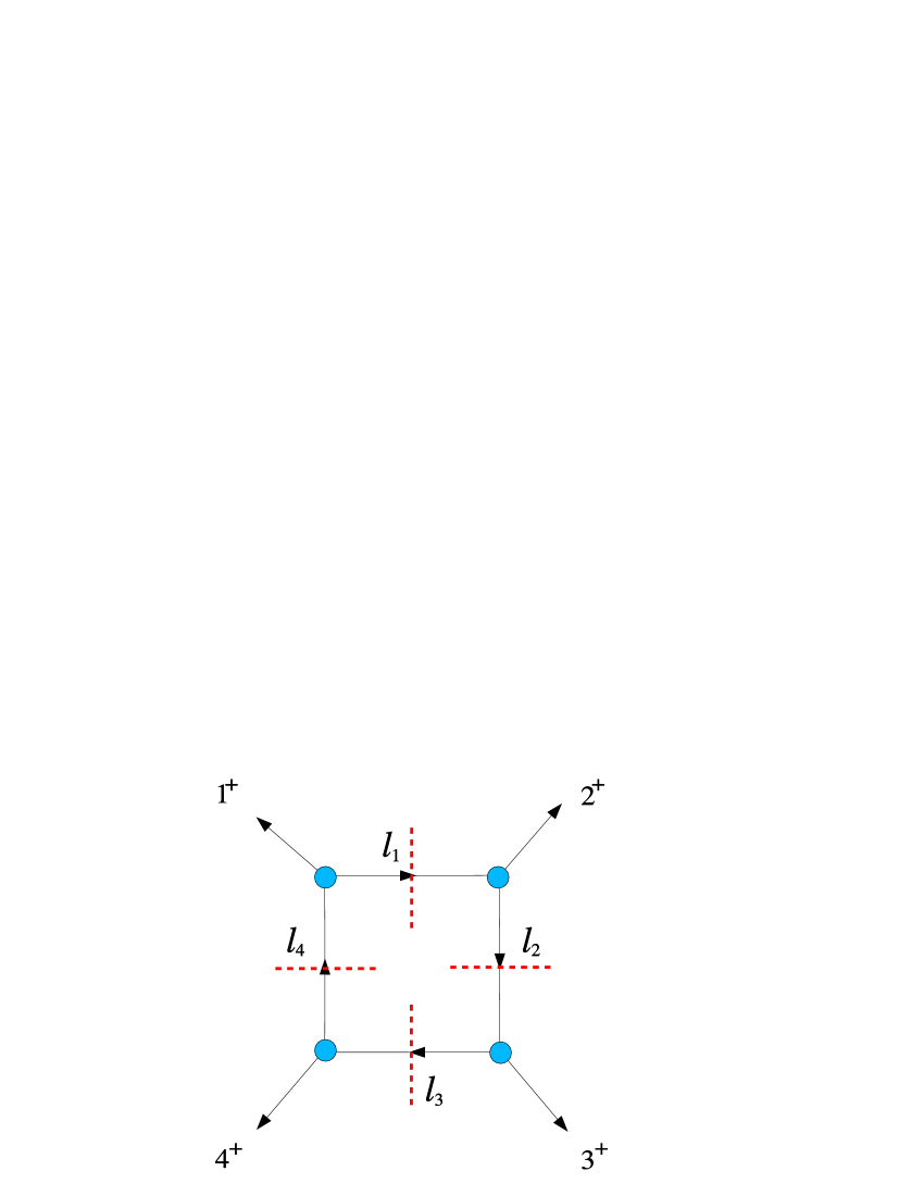
Figure 1: One of the two quadruple-cut diagrams for the amplitude $1^{+}2^{+}3^{+}4^{+}$. This diagrams is obtained by sewing tree amplitudes (represented by the blue bubbles) with an external positive-helicity gluon and two internal scalars of opposite “helicities”. There are two such diagrams, which are obtained one from the other by flipping all the internal helicities. These diagrams are equal so that the full result is obtained by doubling the contribution from the diagram in this Figure. The same remark applies to all the other diagrams considered in this paper.

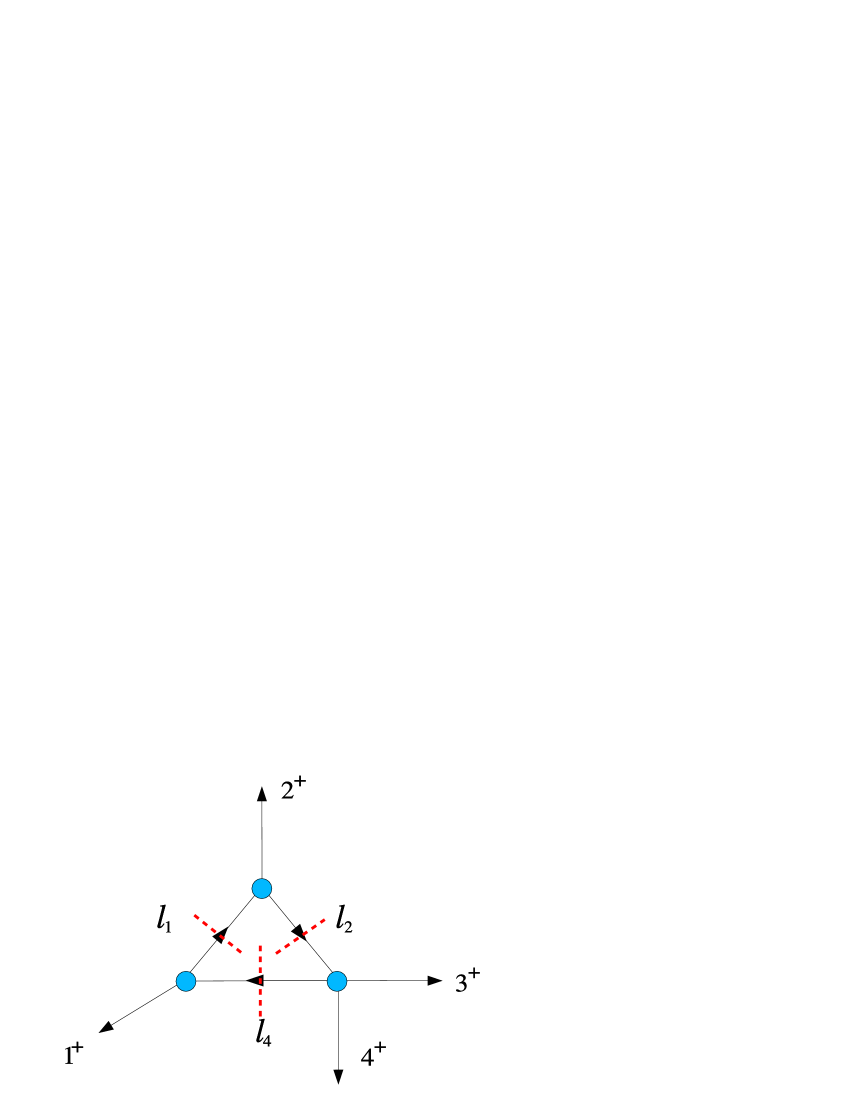
Figure 2: One of the possible three-particle cut diagrams for the amplitude $1^{+}2^{+}3^{+}4^{+}$. The others are obtained from this one by cyclic relabeling of the external particles.

Consider the quadruple-cut diagram in Figure 1, which is obtained by sewing four three-point scattering amplitudes with one massless gluon and two massive scalars of mass $\mu^{2}$. From [11] we take the three-point amplitudes for one positive-helicity gluon and two scalars:

$${\cal A}(l_{1}^{+},k^{+},l_{2}^{-})\ =\ {\cal A}(l_{1}^{-},k^{+},l_{2}^{+})\ =\ {\langle q|l_{1}|k]\over\langle qk\rangle}\ ,$$ (3.7)

where $l_{1}+l_{2}+k=0$. Here $|q\rangle$ is an arbitrary reference spinor not proportional to $|k\rangle$. It is easy to see [11] that (3.7) is actually independent of the choice of $|q\rangle$.

The $D$-dimensional quadruple cut of the amplitude $+$$+$$+$$+$ is obtained by combining four three-point tree-level amplitudes,

$$\frac{\langle q_{1}|l_{1}|1]}{\langle q_{1}1\rangle}\ \frac{\langle q_{2}|l_{2}|2]}{\langle q_{2}2\rangle}\ \frac{\langle q_{3}|l_{3}|3]}{\langle q_{3}3\rangle}\ \frac{\langle q_{4}|l_{4}|4]}{\langle q_{4}4\rangle}\ .$$ (3.8)

The reference momenta $q_{i},i=1,\ldots,4$ in each of the four ratios in this expression may be chosen arbitrarily. Then, using momentum conservation,

$$l_{2}=l_{1}-k_{2}\ ,\qquad l_{4}=l_{3}-k_{4}\ ,$$ (3.9)

the fact that the external momenta are null, and that the internal momenta square to $\mu^{2}$, it is easy to see that

$$\frac{\langle q_{1}|l_{1}|1]}{\langle q_{1}1\rangle}\ \frac{\langle q_{2}|l_{2}|2]}{\langle q_{2}2\rangle}\ =-\mu^{2}{[12]\over\langle 12\rangle}\ ,$$ (3.10)

and similarly

$$\frac{\langle q_{3}|l_{3}|3]}{\langle q_{3}3\rangle}\ \frac{\langle q_{4}|l_{4}|4]}{\langle q_{4}4\rangle}\ =-\mu^{2}{[34]\over\langle 34\rangle}\ ,$$ (3.11)

so that the above expression (3.8) becomes simply

$$\mu^{4}\,\frac{[12][34]}{\langle 12\rangle\langle 34\rangle}\ .$$ (3.12)

Finally, we lift the quadruple-cut box to a box function by reinstating the appropriate Feynman propagators. These propagators then combine with the additional factor of $\mu^{4}$ in (3.12) to yield the factor $iK_{4}/{(4\pi)^{2-\epsilon}}$ which is proportional to the scalar box integral defined in (3.2). Including an additional factor of 2 due to the fact that there is a complex scalar propagating in the loop, the amplitude (3.1) is reproduced correctly.

Next we inspect three-particle cuts. One of the three tree-level amplitudes we sew in the triple-cut amplitude is an amplitude with two positive-helicity gluons and two scalars [39]

$${\cal A}(l_{1}^{+},1^{+},2^{+},l_{2}^{-})\ =\ \mu^{2}{[12]\over\langle 12\rangle[(l_{1}+k_{1})^{2}-\mu^{2}]}\ .$$ (3.13)

Consider, for example, the three-particle cut defined by $1^{+},2^{+},(3^{+},4^{+})$, see Figure 2. Using (3.7) and (3.13), the product of the three tree-level amplitudes gives

$$\frac{\langle q_{1}|l_{1}|1]}{\langle q_{1}1\rangle}\ \frac{\langle q_{2}|l_{1}|2]}{\langle q_{2}2\rangle}\ {\mu^{2}[34]\over\langle 34\rangle[(l_{2}-k_{3})^{2}-\mu^{2}]}\ ,$$ (3.14)

with $l_{2}=l_{1}-k_{2}$. As for the quadruple cut, it is easily seen that, on this triple cut,

$$\frac{\langle q_{1}|l_{1}|1]}{\langle q_{1}1\rangle}\ \frac{\langle q_{2}|l_{1}|2]}{\langle q_{2}2\rangle}\ =\ -\mu^{2}{[12]\over\langle 12\rangle}\ ,$$ (3.15)

where we used $l_{1}^{2}=l_{2}^{2}=l_{4}^{2}=\mu^{2}$. The triple-cut integrand then becomes

$$-{[12][34]\over\langle 12\rangle\langle 34\rangle}{\mu^{4}\over[(l_{2}-k_{3})^{2}-\mu^{2}]}\ ,$$ (3.16)

which, after replacing the three $\delta^{(+)}$ functions by propagators, integrates to (3.1), where we have included an additional $(-1)$ factor following the comments in footnote 6. The factor of $2$ in (3.1) comes from summing over the two “scalar helicities”. The same result comes from evaluating the remaining triple cuts.

We remark that in the case of the quadruple cut we did not even need to insert the solutions of the on-shell conditions for the loop momenta into the expression coming from the cut. This is not true in general; for example, for the five gluon amplitude discussed below the sum over solutions will be essential to obtaining the correct amplitude.

3.2 The one-loop $-$$+$$+$$+$ amplitude

The one-loop four gluon scattering amplitude $-$$+$$+$$+$, with a complex scalar running in the loop, is given to all orders in $\epsilon$ by [38]

$${\cal A}_{4}^{\rm scalar}(1^{-},2^{+},3^{+},4^{+}) = \frac{2i}{(4\pi)^{2-\epsilon}}{[24]^{2}\over[12]\langle 23\rangle\langle 34\rangle[41]}{st\over u}\,\biggl{[}{t(u-s)\over su}J_{3}(s)+{s(u-t)\over tu}J_{3}(t)$$

$$- {t-u\over s^{2}}J_{2}(s)-{s-u\over t^{2}}J_{2}(t)+{st\over 2u}J_{4}+K_{4}\biggr{]}\ .$$

We will now show how to derive this result using generalised unitarity cuts.

First consider the quadruple cut (see Figure 3).

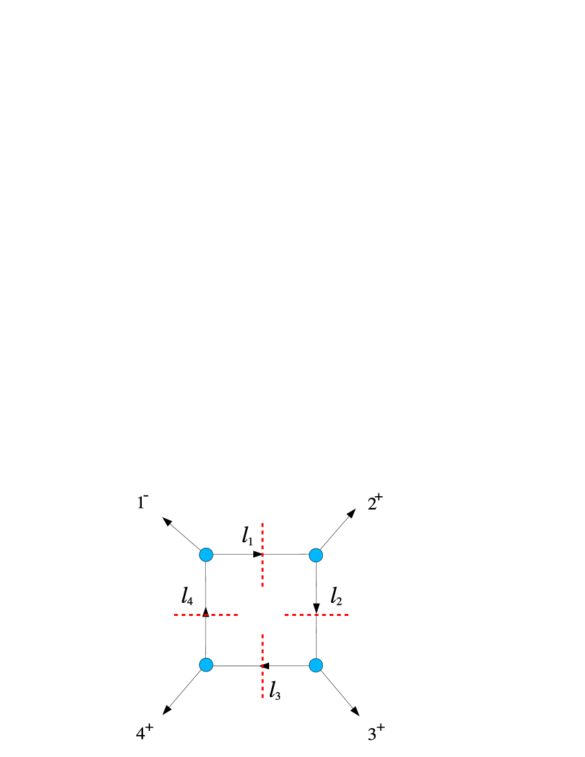
Figure 3: The quadruple cut for the amplitude $1^{-}2^{+}3^{+}4^{+}$.

The product of tree amplitudes gives

$$\frac{\langle 1|l_{1}|q_{1}]}{[1q_{1}]}\ \frac{\langle q_{2}|l_{2}|2]}{\langle q_{2}2\rangle}\ \frac{\langle q_{3}|l_{3}|3]}{\langle q_{3}3\rangle}\ \frac{\langle q_{4}|l_{4}|4]}{\langle q_{4}4\rangle}\ .$$ (3.18)

It is straightforward to show that, on the quadruple cut,

$$\frac{\langle q_{3}|l_{3}|3]}{\langle q_{3}3\rangle}\ \frac{\langle q_{4}|l_{4}|4]}{\langle q_{4}4\rangle} = -\mu^{2}\frac{[34]}{\langle 34\rangle}\ ,$$

$$\frac{\langle 1|l_{1}|q_{1}]}{\langle 1q_{1}\rangle}\ \frac{\langle q_{2}|l_{2}|2]}{\langle q_{2}2\rangle} = \frac{[23]}{[31]}\bigg{(}-\mu^{2}\frac{\langle 31\rangle}{\langle 23\rangle}\,-\,[2|l_{1}|1\rangle\bigg{)}\ ,$$

and hence the quadruple cut in Figure 3 gives

$$Q(1^{+},2^{+},3^{+},4^{-})=\mu^{2}{[3\,4]\over\langle 3\,4\rangle}\,{[2\,3]\over[3\,1]}\left[\mu^{2}{\langle 3\,1\rangle\over\langle 2\,3\rangle}\ +\ [2|l_{1}|1\rangle\right]\ .$$ (3.19)

In order to compare with (3.2) it is useful to notice that

$${[34]\over\langle 34\rangle}{[23]\over[31]}{\langle 31\rangle\over\langle 23\rangle}\ =\ {[24]^{2}\over[12]\langle 23\rangle\langle 34\rangle[41]}{st\over u}\ :=\ {\cal N}\ .$$ (3.20)

We conclude that the first term in (3.19) generates

$$\frac{i}{(4\pi)^{2-\epsilon}}\,\left({[24]^{2}\over[12]\langle 23\rangle\langle 34\rangle[41]}{st\over u}\right)\ K_{4}\ ,$$ (3.21)

where the prefactor in (3.21) comes from the definition (3.2) and (3.3) for the function $K_{4}$.

The second term in (3.19) corresponds to a linear box integral, which we examine now. We notice that the quadruple cut freezes the loop integration on the solution for the cut. In the linear box term in (3.19) we will then replace $l_{1}$ in $[2|l_{1}|1\rangle$ by the solutions of the cut, and sum over the different solutions.

Specifically, in order to solve for the cut-loop momentum $l_{1}$ one has to require

$$l_{1}^{2}\,=\,l_{2}^{2}\,=\,l_{3}^{2}\,=\,l_{4}^{2}\,=\,\mu^{2}\ ,$$

$$l_{1}\,=\,l_{4}-k_{1}\ ,\ l_{2}\,=\,l_{1}-k_{2}\ ,\ l_{3}\,=\,l_{2}-k_{3}\ ,\ l_{4}\,=\,l_{3}-k_{4}\ .$$ (3.22)

In order to solve these conditions, it proves useful [43] to use the four linearly independent vectors $k_{1},k_{2},k_{3}$ and $K$, where

$$K_{\mu}\ :=\ \epsilon_{\mu\nu\rho\sigma}\,k_{1}^{\nu}\,k_{2}^{\rho}\,k_{3}^{\sigma}\ .$$ (3.23)

Setting

$$l_{1}\ =\ ak_{1}\,+\,bk_{2}\,+\,ck_{3}\,+\,dK\ ,$$ (3.24)

one finds

$$a\,=\,\frac{t}{2u}\,,\ b\,=\,\frac{1}{2}\,,\ c\,=\,-\frac{s}{2u}\,,$$ (3.25)

$$d\,=\,\pm\sqrt{-{st+4\mu^{2}u\over stu^{2}}}\,,$$

where

$$s\,=\,(k_{1}+k_{2})^{2}\ ,\ t\,=\,(k_{2}+k_{3})^{2}\ ,\ u\,=\,(k_{1}+k_{3})^{2}\ ,$$ (3.26)

and $s+t+u=0$.

Then one has

$$[2|l_{1}|1\rangle\longrightarrow[2|{l_{1}^{+}+l_{1}^{-}\over 2}|1\rangle\ =\ c\cdot[2|3|1\rangle\ =\ -{s\over 2u}[23]\langle 31\rangle\ ,$$ (3.27)

where $l_{1}^{\pm}$ denotes the two solutions for the quadruple cut. The square root drops out of the calculation (as it should, given that the amplitude is a rational function). We conclude that the second term in (3.19) gives

$$\frac{i}{(4\pi)^{2-\epsilon}}\,\left({[24]^{2}\over[12]\langle 23\rangle\langle 34\rangle[41]}{st\over u}\right)\ {st\over 2u}J_{4}\ ,$$ (3.28)

where

$$J_{n}\ :=\ I_{n}[\mu^{2}]\ .$$ (3.29)

Again, the prefactor in (3.28) arises from the definition (3.3).

In total the quadruple cut (3.19) gives

$$\frac{2i}{(4\pi)^{2-\epsilon}}\,{\cal N}\left(K_{4}\ +\ {st\over 2u}J_{4}\right)\ ,$$ (3.30)

where we have again included a factor of two for the contribution of a complex scalar. This result matches exactly all the box functions appearing in (3.2).

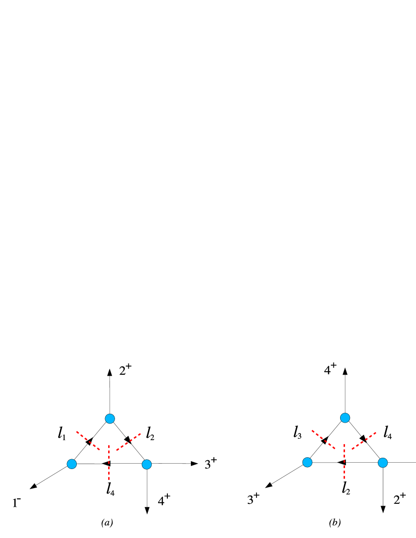
Figure 4: The two inequivalent triple cuts for the amplitude $1^{-}2^{+}3^{+}4^{+}$.

We now move on to consider triple cuts. We start by considering the triple cut in Figure 4a, which we label as $(1^{-},2^{+},(3^{+},4^{+}))$. It may be shown that this triple cut yields the following expression:

$$TC(1^{-},2^{+},(3^{+},4^{+})) = \mu^{2}{[3\,4]\over\langle 3\,4\rangle}\,{[2\,3]\over[3\,1]}\left(-\mu^{2}{\langle 3\,1\rangle\over\langle 2\,3\rangle}\ -\ [2|l_{1}|1\rangle\right){1\over(l_{2}-k_{3})^{2}-\mu^{2}}\$$

$$\qquad-\mu^{2}\,{[3\,4]\over\langle 3\,4\rangle}{[2|l_{1}|1\rangle\over\langle 2\,3\rangle[3\,1]}\ .$$ (3.31)

The first line in (3.2) clearly contains the (negative of the) term already studied with quadruple cuts – see (3.19) (for an explanation of the relative minus sign see footnote 6). We now reconsider the linear box term (second term in the first line of (3.2)), and study its Passarino-Veltman (PV) reduction. As we shall see, this box appears also in other triple cuts (see (3.2)).

Let us consider the linear box integral

$$A^{\mu}\ :=\ \int\!\!{d^{4}l_{1}\over(2\pi)^{4}}{d^{-2\epsilon}\mu\over(2\pi)^{-2\epsilon}}{\mu^{2}\ l_{1}^{\mu}\over(l_{1}^{2}-\mu^{2})[(l_{1}-k_{2})^{2}-\mu^{2}][(l_{1}-k_{2}-k_{3})^{2}-\mu^{2}][(l_{1}+k_{1})^{2}-\mu^{2}]}\ .$$ (3.32)

On general grounds the integral is a linear combination of three of the external momenta,

$$A^{\mu}\ =\ \alpha k_{1}^{\mu}\,+\,\beta k_{2}^{\mu}+\,\gamma k_{3}^{\mu}\ .$$ (3.33)

For the coefficients we find

$$\alpha = -{i\over(4\pi)^{2-\epsilon}}\ {1\over 2u}\Big{[}-tJ_{4}\,-\,2J_{3}(s)\,+\,2J_{3}(t)\Big{]}\ ,$$ (3.34)

$$\beta = {i\over(4\pi)^{2-\epsilon}}\ {1\over 2}J_{4}\ ,$$

$$\gamma = -{i\over(4\pi)^{2-\epsilon}}\ {1\over 2u}\Big{[}sJ_{4}\,-\,2J_{3}(s)\,+\,2J_{3}(t)\Big{]}\ .$$

Taken literally, this means that from the linear box in (3.2) we not only get the $J_{4}$ function but, altogether:

$$\,\frac{i{\cal N}}{(4\pi)^{2-\epsilon}}\left({st\over 2u}J_{4}\,-\,{t\over u}J_{3}(s)\,+\,{t\over u}J_{3}(t)\right)\ .$$ (3.35)

Summarising, the PV reduction of the first line of the triple cut (3.2), lifted to a Feynman integral, gives:

$$\frac{i{\cal N}}{(4\pi)^{2-\epsilon}}\left(K_{4}\,+\,{st\over 2u}J_{4}\,-\,{t\over u}J_{3}(s)\,+\,{t\over u}J_{3}(t)\right)\ .$$ (3.36)

The last term in (3.36) is clearly spurious – it does not have the right triple cut, and has appeared because we lifted the cut-integral to a Feynman integral; hence we will drop it. In conclusion, the triple cut $(1^{-},2^{+},(3^{+},4^{+}))$ in Figure 4a leads to

$$\frac{i{\cal N}}{(4\pi)^{2-\epsilon}}\left(K_{4}\,+\,{st\over 2u}J_{4}\,-\,{t\over u}J_{3}(s)\right)\ .$$ (3.37)

We now consider the last term in (3.2), which generates a linear triangle, whose PV reduction we consider now. The linear triangle is proportional to

$$B^{\mu}\ :=\ \int\!\!{d^{4}l_{1}\over(2\pi)^{4}}{d^{-2\epsilon}\mu\over(2\pi)^{-2\epsilon}}{\mu^{2}\,l_{1}^{\mu}\over(l_{1}^{2}-\mu^{2})[(l_{1}-k_{2})^{2}-\mu^{2}][(l_{1}+k_{1})^{2}-\mu^{2}]}\ .$$ (3.38)

On general grounds,

$$B^{\mu}\ =\ \theta k_{1}^{\mu}\,+\,\tau k_{2}^{\mu}\ ,$$ (3.39)

and hence

$$[2|\,B\,|1\rangle\ \ =\ 0\ .$$ (3.40)

We conclude that the second line in (3.2) gives a vanishing contribution, so that the content of this triple cut is encoded in (3.37).

Next we consider the triple cut labelled by $((1^{-},2^{+}),3^{+},4^{+})$ and represented in Figure 4b, which gives

$$TC((1^{-},2^{+}),3^{+},4^{+}) = \mu^{2}{[3\,4]\over\langle 3\,4\rangle}{[2\,3]\over[3\,1]}\left[-\mu^{2}{\langle 3\,1\rangle\over\langle 2\,3\rangle}\ +\ {\langle 1\,2\rangle\over\langle 2\,3\rangle}\,\langle 3|l_{2}|2]\right]{1\over(l_{2}+k_{2})^{2}-\mu^{2}}\$$ (3.41)

$$\qquad+\mu^{2}{[3\,4]\over\langle 3\,4\rangle}\,{\langle 1|3\,1\,l_{2}-2\,3\,l_{2}|2]\over\langle 1\,2\,\rangle[1\,2]\,\langle 2\,3\rangle\,[3\,1]}\ .$$

The first term of (3.41) clearly corresponds to the function $K_{4}$ already fixed using quadruple cuts. The second term can be rewritten as follows. Introducing $l_{1}:=l_{2}+k_{2}$, we have

$${\langle 12\rangle\over\langle 23\rangle}\langle 3|l_{2}|2]\ =\ -\,[2|l_{2}|1\rangle\,+\,{\langle 13\rangle\over\langle 23\rangle}\,[(l_{2}+k_{2})^{2}-\mu^{2}]\ ,$$ (3.42)

therefore we can rewrite (3.41) as

$$TC((1^{-},2^{+}),3^{+},4^{+}) = \mu^{2}{[3\,4]\over\langle 3\,4\rangle}\,{[2\,3]\over[3\,1]}\left(-\mu^{2}{\langle 3\,1\rangle\over\langle 2\,3\rangle}\ -\ [2|l_{1}|1\rangle\right){1\over(l_{2}+k_{2})^{2}-\mu^{2}}\$$

$$+ \mu^{2}{[3\,4]\over\langle 3\,4\rangle}\,\biggl{(}{\langle 1|3\,1\,l_{2}-2\,3\,l_{2}|2]\over\langle 1\,2\,\rangle[1\,2]\,\langle 2\,3\rangle\,[3\,1]}\,-\,{[23]\over[31]}{\langle 31\rangle\over\langle 23\rangle}\biggr{)}\ .$$ (3.43)

We know already that the PV reduction of the first line of (3.2) corresponds to (3.36) – with the term containing $J_{3}(t)$ removed – so we now study the second line, which will give new contributions.

The second term in the second line corresponds to a scalar triangle, more precisely it gives a contribution

$$-\,\frac{i{\cal N}}{(4\pi)^{2-\epsilon}}\,J_{3}(s)\ .$$ (3.44)

The first term corresponds to a linear triangle, and now we perform its PV reduction. The relevant integral is

$$C^{\mu}\ :=\ \int\!\!{d^{4}l_{2}\over(2\pi)^{4}}{d^{-2\epsilon}\mu\over(2\pi)^{-2\epsilon}}{\mu^{2}\,l_{2}^{\mu}\over(l_{2}^{2}-\mu^{2})[(l_{2}-k_{3})^{2}-\mu^{2}][(l_{2}+k_{1}+k_{2})^{2}-\mu^{2}]}\ .$$ (3.45)

On general grounds,

$$C^{\mu}\ =\ \lambda\,k_{3}^{\mu}\ +\ \kappa\,(k_{1}+k_{2})^{\mu}\ .$$ (3.46)

A quick calculation shows that

$$\lambda\ =-{i\over(4\pi)^{2-\epsilon}}\ \Bigl{[}J_{3}(s)\,-\,{2\over s}J_{2}(s)\Bigr{]}\ ,\qquad\kappa\ =\ {i\over(4\pi)^{2-\epsilon}}\ {1\over s}J_{2}(s)\ .$$ (3.47)

The first term in the second line of (3.2) gives then

$$\frac{i{\cal N}}{(4\pi)^{2-\epsilon}}\ \left(-{u\over s}\,J_{3}(s)\,+\,{u-t\over s}\,J_{2}(s)\right)\ ,$$ (3.48)

where ${\cal N}$ is defined in (3.20). Altogether, the second line of (3.2) gives

$$\frac{i{\cal N}}{(4\pi)^{2-\epsilon}}\ \left(-\Big{(}1\,+{u\over s}\Big{)}\,J_{3}(s)\,+\,{u-t\over s}\,J_{2}(s)\right)\ ,$$ (3.49)

whereas from the first line of the same equation we get

$$\frac{i{\cal N}}{(4\pi)^{2-\epsilon}}\left(K_{4}\,+\,{st\over 2u}J_{4}\,-\,{t\over u}J_{3}(s)\right)\ ,$$ (3.50)

where we have dropped the term $J_{3}(t)$ for reasons explained earlier.

We conclude that the function which incorporates all the right cuts in the channels considered so far is equal to the sum of (3.49) and (3.50), which gives

$$\frac{i{\cal N}}{(4\pi)^{2-\epsilon}}\left(K_{4}\,+\,{st\over 2u}J_{4}\,-\,{t\over u}\,J_{3}(s)\,-\,\Big{(}1\,+{u\over s}\Big{)}\,J_{3}(s)\,+\,{u-t\over s^{2}}\,J_{2}(s)\right)\ .$$ (3.51)

Using $-t/u-1-u/s=s/u-u/s$, (3.51) becomes

$$\frac{i{\cal N}}{(4\pi)^{2-\epsilon}}\left(K_{4}\,+\,{st\over 2u}J_{4}\,+\,\Big{(}{s\over u}\,-\,{u\over s}\Big{)}\,J_{3}(s)\,+\,{u-t\over s^{2}}\,J_{2}(s)\right)\ .$$ (3.52)

To finish the calculation one has to consider the two remaining triple cuts, that is $(4^{+},1^{-},(2^{+},3^{+}))$ and $((4^{+},1^{-}),2^{+},3^{+})$. These cuts can be obtained from the previously considered cuts by exchanging $s$ with $t$.

Our conclusion is therefore that the function (including the usual factor of 2) with the correct quadruple and triple cuts is:

$$\frac{2i{\cal N}}{(4\pi)^{2-\epsilon}}\left(K_{4}\,+\,{st\over 2u}J_{4}+\Big{(}{s\over u}\,-\,{u\over s}\Big{)}\,J_{3}(s)\,+\,{u-t\over s^{2}}\,J_{2}(s)\right.$$ (3.53)

$$\qquad\qquad\qquad\qquad+\left.\Big{(}{t\over u}\,-\,{u\over t}\Big{)}\,J_{3}(t)\,+\,{u-s\over t^{2}}\,J_{2}(t)\right)\ .$$

This agrees precisely with (3.1) using the identities

$${t(u-s)\over su}\ =\ {s\over u}\,-\,{u\over s}\ ,\qquad{s(u-t)\over tu}\ =\ {t\over u}\,-\,{u\over t}\ .$$ (3.54)

3.3 The one-loop $-$$-$$+$$+$ amplitude

We now turn our attention to the one-loop four point amplitudes with two negative helicity gluons. We start by considering the one-loop amplitude ${\cal A}^{\rm scalar}_{4}(1^{-},2^{-},3^{+},4^{+})$, which is given by [38]

$${\cal A}^{\rm scalar}_{4}(1^{-},2^{-},3^{+},4^{+})=2\frac{{\cal A}_{4}^{\rm tree}}{(4\pi)^{2-\epsilon}}\bigg{(}-\frac{t}{s}K_{4}+\frac{1}{s}J_{2}(t)+\frac{1}{t}I_{2}^{6-2\epsilon}(t)\bigg{)}\ .$$ (3.55)

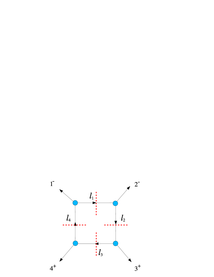
Figure 5: The quadruple cut for the amplitude $1^{-}2^{-}3^{+}4^{+}$.

To begin with, we consider the quadruple cut of the amplitude, represented in Figure 5. It is given by

$$\frac{\langle 1|l_{1}|q_{1}]}{[1\,q_{1}]}\ \frac{\langle 2|l_{1}|q_{2}]}{[2\,q_{2}]}\ \frac{\langle q_{3}|l_{3}|3]}{\langle q_{3}\,3\rangle}\ \frac{\langle q_{4}|l_{4}|4]}{\langle q_{4}\,4\rangle}\ .$$ (3.56)

By choosing $q_{1}=2$, $q_{2}=1$, $q_{3}=4$, $q_{4}=3$, (3.56) can be rewritten as

$$i\,{t\over s}\,{\cal A}_{4}^{\rm tree}\,\mu^{4}\ ,$$ (3.57)

where

$${\cal A}_{4}^{\rm tree}\ =\ i\frac{\langle 1\,2\rangle^{3}}{\langle 2\,3\rangle\langle 3\,4\rangle\langle 4\,1\rangle}\ .$$ (3.58)

Reinstating the four cut propagators and integrating over the loop momentum, (3.57) gives

$$-\frac{{\cal A}_{4}^{\rm tree}}{(4\pi)^{2-\epsilon}}\bigg{(}\frac{t}{s}K_{4}\bigg{)}\ ,$$ (3.59)

where $K_{4}$ is defined in (3.2).

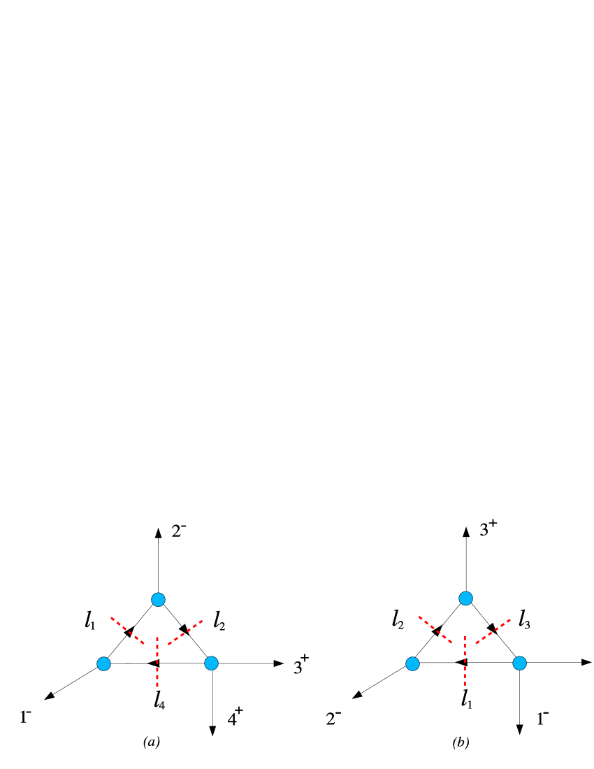
Figure 6: The two inequivalent triple cuts for the amplitude $1^{-}2^{-}3^{+}4^{+}$.

Next we consider triple cuts. We begin our analysis with the triple cut in Figure 6a. This yields

$$\frac{\mu^{2}[3\,4]}{\langle 3\,4\rangle 2(l_{2}\cdot 3)}\ \frac{\langle 1|l_{1}|q_{1}]}{[1\,q_{1}]}\ \frac{\langle 2|l_{1}|q_{2}]}{[2\,q_{2}]}\ =\ -\mu^{4}\frac{\langle 1\,2\rangle[3\,4]}{[1\,2]\langle 3\,4\rangle}\ \frac{1}{2(l_{2}\cdot 3)}\ ,$$ (3.60)

which, upon reinstating the cut propagators and performing the loop momentum integration gives

$$-\frac{{\cal A}_{4}^{\rm tree}}{(4\pi)^{2-\epsilon}}\bigg{(}\frac{t}{s}K_{4}\bigg{)}\ .$$ (3.61)

This function had already been detected with the quadruple cut, as discussed earlier.

Next we move on to consider the triple cut in Figure 6b. This yields

$$\frac{\langle 1|l_{3}|4]^{2}}{2\,t\,(l_{3}\cdot 4)}\ \frac{\langle 2|l_{1}|q_{1}]}{[2\,q_{1}]}\ \frac{\langle q_{2}|l_{2}|3]}{\langle q_{2}\,3\rangle}\ .$$ (3.62)

We can re-cast (3.62) as follows. Firstly, we write

$$\frac{\langle 1|l_{3}|4]\langle q_{2}|l_{3}|3]}{\langle q_{2}\,3\rangle}\ =\ \mu^{2}\frac{\langle 1|4|3]}{\langle 3\,4\rangle}-\frac{2(l_{3}\cdot 4)\langle 1|l_{3}|3]}{\langle 3\,4\rangle}\ ,$$ (3.63)

and secondly

$$\frac{\langle 1|l_{3}|4]\langle 2|l_{1}|q_{1}]}{[2\,q_{1}]}\ =\ \mu^{2}\frac{\langle 2|1|4]}{[1\,2]}-\frac{2(l_{3}\cdot 4)\langle 2|1|4]}{[1\,2]}+\frac{2(l_{3}\cdot 4)\langle 2|l_{3}|4]}{[1\,2]}\ .$$ (3.64)

The expression (3.62) becomes a sum of six terms $T_{i}$, $i=1,\ldots,6$, where

$$T_{1} = \frac{\langle 1|4|3]\langle 2|1|4]\mu^{4}}{t\langle 3\,4\rangle[1\,2]2(l_{3}\cdot 4)}\ ,$$

$$T_{2} = -\frac{\langle 1|4|3]\langle 2|1|4]\mu^{2}}{t\langle 3\,4\rangle[1\,2]}\ ,$$

$$T_{3} = \frac{\langle 1|4|3]\langle 2|l_{3}|4]\mu^{2}}{t\langle 3\,4\rangle[1\,2]}\ ,$$

$$T_{4} = -\frac{\langle 2|1|4]\langle 1|l_{3}|3]\mu^{2}}{t\langle 3\,4\rangle[1\,2]}\ ,$$

$$T_{5} = \frac{\langle 2|1|4]\langle 1|l_{3}|3]2(l_{3}\cdot 4)}{t\langle 3\,4\rangle[1\,2]}\ ,$$

$$T_{6} = -\frac{\langle 1|l_{3}|3]\langle 2|l_{3}|4]2(l_{3}\cdot 4)}{t\langle 3\,4\rangle[1\,2]}\ .$$ (3.65)

Next we replace the delta functions with propagators, and integrate over the loop momentum. To evaluate the integrals, we use the linear, quadratic and cubic triangle integrals in $4-2\epsilon$ dimensions listed in the Appendix. The integration of the expressions gives

$$T_{1} \to -{{\cal A}_{4}^{\rm tree}\over(4\pi)^{2-\epsilon}}\bigg{(}\frac{t}{s}K_{4}\bigg{)}\ ,$$

$$T_{2} \to -{{\cal A}_{4}^{\rm tree}\over(4\pi)^{2-\epsilon}}\bigg{(}-\frac{t}{s}J_{3}(t)\bigg{)}\ ,$$

$$T_{3} \to -{{\cal A}_{4}^{\rm tree}\over(4\pi)^{2-\epsilon}}\bigg{(}\frac{t}{s}J_{3}(t)-\frac{1}{s}J_{2}(t)\bigg{)}\ ,$$

$$T_{4} \to -{{\cal A}_{4}^{\rm tree}\over(4\pi)^{2-\epsilon}}\bigg{(}-\frac{1}{s}J_{2}(t)\bigg{)}\ ,$$

$$T_{5} \to -{{\cal A}_{4}^{\rm tree}\over(4\pi)^{2-\epsilon}}\bigg{(}\frac{t}{2s}I_{2}(t)+\frac{u}{s}I_{3}^{6-2\epsilon}(t)\bigg{)}\ ,$$

$$T_{6} \to -{{\cal A}_{4}^{\rm tree}\over(4\pi)^{2-\epsilon}}\bigg{(}-\frac{t}{4s}I_{2}(t)-\bigg{(}\frac{3}{2s}+\frac{1}{t}\bigg{)}I_{2}^{6-2\epsilon}(t)-\frac{u}{s}I_{3}^{6-2\epsilon}(t)\bigg{)}\ .$$ (3.66)

We now use (A.26) in [38] relating $J_{2}(t)$ to $I_{2}(t)$ and $I_{2}^{6-2\epsilon}(t)$, and get

$$T_{5}+T_{6}\to-{\cal A}_{4}^{\rm tree}\bigg{(}\frac{1}{s}J_{2}(t)-\frac{1}{t}I_{2}^{6-2\epsilon}(t)\bigg{)}\ .$$ (3.67)

Adding up the six $T_{i}$ terms, and including the usual factor of two, we obtain

$$-{2{\cal A}_{4}^{\rm tree}\over(4\pi)^{2-\epsilon}}\bigg{(}\frac{t}{s}K_{4}-\frac{1}{s}J_{2}(t)-\frac{1}{t}I_{2}^{6-2\epsilon}(t)\bigg{)}\ ,$$ (3.68)

which precisely agrees with (3.55).

3.4 The one-loop $-$$+$$-$$+$ amplitude

Now we consider the one-loop amplitude with a complex scalar in the loop, ${\cal A}^{\rm scalar}_{4}(1^{-},2^{+},3^{-},4^{+})$, which is given by [38]

$${\cal A}_{4}^{\rm scalar}(1^{-},2^{+},3^{-},4^{+}) = -2\frac{1}{(4\pi)^{2-\epsilon}}{\cal A}_{4}^{\rm tree}\bigg{(}\frac{st}{u^{2}}K_{4}-\frac{s^{2}t^{2}}{u^{3}}I_{4}^{6-2\epsilon}+\frac{st}{u^{2}}I_{3}^{6-2\epsilon}(t)$$

$$+ \frac{st}{u^{2}}I_{3}^{6-2\epsilon}(s)-\frac{st(s-t)}{u^{3}}J_{3}(t)-\frac{st(t-s)}{u^{3}}J_{3}(s)+\frac{s}{u^{2}}J_{2}(t)+\frac{t}{u^{2}}J_{2}(s)$$

$$+ \frac{s}{tu}I_{2}^{6-2\epsilon}(t)+\frac{t}{su}I_{2}^{6-2\epsilon}(s)+\frac{ts^{2}}{u^{3}}I_{2}(t)+\frac{st^{2}}{u^{3}}I_{2}(s)\bigg{)}\ .$$

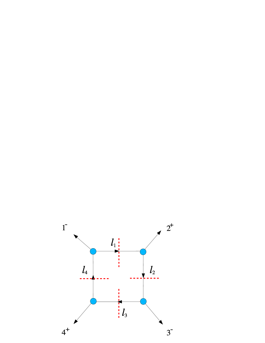
Figure 7: The quadruple cut for the amplitude $1^{-}2^{+}3^{-}4^{+}$.

The relevant quadruple cut is represented in Figure 7, and gives:

$$\frac{\langle 1|l_{1}|q_{1}]}{[1\,q_{1}]}\ \frac{\langle q_{2}|l_{2}|2]}{\langle q_{2}\,2\rangle}\ \frac{\langle 3|l_{3}|q_{3}]}{[3\,q_{3}]}\ \frac{\langle q_{4}|l_{4}|q_{4}]}{\langle q_{4}\,4\rangle}\$$

$$=\frac{1}{[1\,3]\langle 2\,4\rangle}\ \bigg{(}\langle 1\,3\rangle\mu^{2}+\langle 1\,2\rangle\langle 3|l_{1}|2]\bigg{)}\bigg{(}[2\,4]\mu^{2}-[3\,4]\langle 3|l_{1}|2]\bigg{)}$$

$$=i{\cal A}_{4}^{\rm{tree}}\bigg{(}\frac{st\mu^{4}}{u^{2}}+\frac{2s^{2}t\langle|l_{1}|2]\mu^{2}}{u^{2}\langle 3|1|2]}+\frac{s^{3}t\langle 3|l_{1}|2]^{2}}{u^{2}\langle 3|1|2]^{2}}\bigg{)}\ ,$$ (3.70)

where

$${\cal A}_{4}^{\rm tree}\ =\ i\frac{\langle 13\rangle^{4}}{\langle 12\rangle\langle 23\rangle\langle 34\rangle\langle 41\rangle}\ .$$ (3.71)

Averaging over the two solutions of the quadruple cut we obtain the following expression:

$$i{\cal A}_{4}^{\rm{tree}}\bigg{(}\frac{st}{u^{2}}\ \mu^{4}+\frac{2s^{2}t^{2}}{u^{3}}\ \mu^{2}+\frac{s^{3}t^{3}}{2u^{4}}\bigg{)}\ .$$ (3.72)

After reinstating the four cut propagators and integrating over the loop momentum, (3.72) gives

$$\frac{1}{(4\pi)^{2-\epsilon}}{\cal A}_{4}^{\rm{tree}}\bigg{(}-\frac{st}{u^{2}}K_{4}-\frac{2s^{2}t^{2}}{u^{3}}J_{4}-\frac{s^{3}t^{3}}{2u^{4}}I_{4}\bigg{)}\ .$$ (3.73)

We now use the identity (A.26) in [38] ignoring functions that do not have a quadruple cut to write this as

$$\frac{1}{(4\pi)^{2-\epsilon}}{\cal A}_{4}^{\rm{tree}}\bigg{(}-\frac{st}{u^{2}}K_{4}+\frac{s^{2}t^{2}}{u^{3}}I_{4}^{6-2\epsilon}\bigg{)}\ .$$ (3.74)

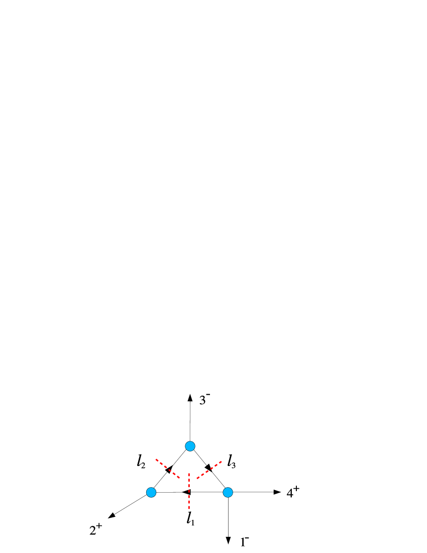
Figure 8: The only independent triple cut for the amplitude $1^{-}2^{+}3^{-}4^{+}$ (the others are obtained from this one by cyclic relabeling of the external gluons).

We now consider triple cuts. There is only one independent triple cut, and we consider, for instance, the triple cut in Figure 8, which gives

$$\frac{\langle 1|l_{3}|4]^{2}}{2\,t\,(l_{3}\cdot 4)}\ \frac{\langle 3|l_{3}|q_{2}]}{[3\,q_{2}]}\ \frac{\langle q_{1}|l_{1}|2]}{\langle q_{1}\,2\rangle}\ .$$ (3.75)

Using straightforward spinor manipulations, and taking into account properties of the cut momenta, one finds that the above expression may be expanded as a product of two sets of terms. The first is

$$\frac{\langle 1|l_{3}|4]\langle 3|l_{3}|q_{2}]}{[3\,q_{2}]}\ =\ \frac{\mu^{2}\langle 3|1|4]}{[1\,3]}-\frac{t\langle 3|l_{3}|4]}{[1\,3]}+\frac{2(l_{3}\cdot 4)\langle 3|l_{3}|4]}{[1\,3]}\ ,$$ (3.76)

whereas the second is

$$\frac{\langle 1|l_{3}|4]\langle q_{1}|l_{1}|2]}{\langle q_{1}\,2\rangle}\ =\ \frac{\mu^{2}\langle 1|4|2]}{\langle 2\,4\rangle}+\frac{\langle 4|1|2]\langle 1|l_{3}|4]}{\langle 2\,4\rangle}-\frac{2(l_{3}.4)\langle 1|l_{3}|2]}{\langle 2\,4\rangle}\ .$$ (3.77)

The expression (3.75) becomes then a sum of nine terms $R_{i}$, $i=1,\ldots,9$, where

$$R_{1} = \frac{\langle 1|4|2]\langle 3|1|4]\mu^{4}}{t[1\,3]\langle 2\,4\rangle 2(l_{3}\cdot 4)}\ ,$$

$$R_{2} = \frac{\langle 4|1|2]\langle 3|1|4]\langle 1|l_{3}|4]\mu^{2}}{t[1\,3]\langle 2\,4\rangle 2(l_{3}\cdot 4)}\ ,$$

$$R_{3} = -\frac{\langle 3|1|4]\langle 1|l_{3}|2]\mu^{2}}{t[1\,3]\langle 2\,4\rangle}\ ,$$

$$R_{4} = -\frac{\langle 1|4|2]\langle 3|l_{3}|4]\mu^{2}}{[1\,3]\langle 2\,4\rangle 2(l_{3}\cdot 4)}\ ,$$

$$R_{5} = -\frac{\langle 4|1|2]\langle 3|l_{3}|4]\langle 1|l_{3}|4]}{[1\,3]\langle 2\,4\rangle 2(l_{3}\cdot 4)}\ ,$$

$$R_{6} = \frac{\langle 3|l_{3}|4]\langle 1|l_{3}|2]}{[1\,3]\langle 2\,4\rangle}\ ,$$

$$R_{7} = \frac{\langle 1|4|2]\langle 3|l_{3}|4]\mu^{2}}{t[1\,3]\langle 2\,4\rangle}\ ,$$

$$R_{8} = \frac{\langle 4|1|2]\langle 3|l_{3}|4]\langle 1|l_{3}|4]}{t[1\,3]\langle 2\,4\rangle}\ ,$$

$$R_{9} = -\frac{\langle 3|l_{3}|4]\langle 1|l_{3}|2]2(l_{3}\cdot 4)}{t[1\,3]\langle 2\,4\rangle}\ .$$ (3.78)

The term $R_{5}$ becomes a quadratic box integral when the three delta functions are replaced with propagators. We can use the properties of the cut momenta to re-write $R_{5}$ as a sum of terms which will give a box integral, a linear box integral and a linear triangle integral as follows,

$$R_{5}=-\frac{\langle 4|1|2][4|3\,1|4]\mu^{2}}{[1\,3]^{2}\langle 2\,4\rangle 2(l_{3}\cdot 4)}+\frac{t\langle 4|1|2][4|3\,l_{3}|4]}{[1\,3]^{2}\langle 2\,4\rangle 2(l_{3}\cdot 4)}-\frac{\langle 4|1|2][4|3\,l_{3}|4]}{[1\,3]^{2}\langle 2\,4\rangle}\ .$$ (3.79)

We now replace the delta functions with propagators and integrate over the cut momenta. Note that one must drop any terms without cuts in the $t$-channel. This must be used for all the linear box integrals that appear above. Using the results for the linear box and the linear, quadratic and cubic triangle integrals in $4-2\epsilon$ dimensions listed in the Appendix gives

$$R_{1} \to -{{\cal A}_{4}^{\rm tree}\over(4\pi)^{2-\epsilon}}\bigg{(}\frac{st}{u^{2}}K_{4}\bigg{)}\ ,$$

$$R_{2} \to -{{\cal A}_{4}^{\rm tree}\over(4\pi)^{2-\epsilon}}\bigg{(}\frac{s^{2}t^{2}}{2u^{3}}J_{4}-\frac{s^{2}t}{u^{3}}J_{3}(t)\bigg{)}\ ,$$

$$R_{3} \to -{{\cal A}_{4}^{\rm tree}\over(4\pi)^{2-\epsilon}}\bigg{(}-\frac{st}{u^{2}}J_{3}(t)+\frac{s}{u^{2}}J_{2}(t)\bigg{)}\ ,$$

$$R_{4} \to -{{\cal A}_{4}^{\rm tree}\over(4\pi)^{2-\epsilon}}\bigg{(}\frac{s^{2}t^{2}}{2u^{3}}J_{4}+\frac{st^{2}}{u^{3}}J_{3}(t)\bigg{)}\ ,$$

$$R_{5} \to -{{\cal A}_{4}^{\rm tree}\over(4\pi)^{2-\epsilon}}\bigg{(}\frac{s^{2}t^{2}}{u^{3}}J_{4}+\frac{s^{3}t^{3}}{2u^{4}}I_{4}+\frac{s^{2}t^{3}}{u^{4}}I_{3}(t)+\frac{s^{2}t}{u^{3}}I_{2}(t)\bigg{)}\ ,$$

$$R_{6} \to -{{\cal A}_{4}^{\rm tree}\over(4\pi)^{2-\epsilon}}\bigg{(}\frac{st}{2u^{2}}I_{2}(t)\bigg{)}\ ,$$

$$R_{7} \to -{{\cal A}_{4}^{\rm tree}\over(4\pi)^{2-\epsilon}}\bigg{(}\frac{s}{u^{2}}J_{2}(t)\bigg{)}\ ,$$

$$R_{8} \to -{{\cal A}_{4}^{\rm tree}\over(4\pi)^{2-\epsilon}}\bigg{(}-\frac{s^{2}}{u^{2}}I_{3}^{6-2\epsilon}(t)\bigg{)}\ ,$$

$$R_{9} \to -{{\cal A}_{4}^{\rm tree}\over(4\pi)^{2-\epsilon}}\bigg{(}-\frac{st}{4u^{2}}I_{2}(t)+\bigg{(}\frac{s}{2u^{2}}-\frac{s^{2}}{u^{2}t}\bigg{)}I_{2}^{6-2\epsilon}(t)+\frac{s^{2}}{u^{2}}I_{3}^{6-2\epsilon}(t)\bigg{)}\ .$$ (3.80)

Now using (A.26) in [38], and ignoring all terms without cuts in the $t$-channel, it is easy to show that the sum of these nine terms leads to the result

$${\cal A}^{\rm t-cut}(1^{-},2^{+},3^{-},4^{+}) = -\frac{1}{(4\pi)^{2-\epsilon}}{\cal A}_{4}^{\rm tree}\bigg{(}\frac{st}{u^{2}}K_{4}-\frac{s^{2}t^{2}}{u^{3}}I_{4}^{6-2\epsilon}+\frac{st}{u^{2}}I_{3}^{6-2\epsilon}(t)$$

$$- \frac{st(s-t)}{u^{3}}J_{3}(t)+\frac{s}{u^{2}}J_{2}(t)+\frac{s}{tu}I_{2}^{6-2\epsilon}(t)+\frac{ts^{2}}{u^{3}}I_{2}(t)\bigg{)}\ .$$

Next, one must also include the corresponding terms coming from the $s$-channel version of the of triple cut in Figure 8. This just yields (3.4) with $t$ replaced by $s$. Combining these two expressions, without double-counting the box contributions (which appear in both cuts), and including the usual factor of two, one precisely reproduces the amplitude for this process (3.4)

4 The $+$$+$$+$$+$$+$ amplitude

The five-gluon all-plus one loop amplitude, with a scalar in the loop, is given by [50]

$${\cal A}_{5}(1^{+},2^{+},3^{+},4^{+},5^{+})\ =\ {i\over 96\pi^{2}C_{5}}\bigg{[}s_{12}s_{23}+s_{23}s_{34}+s_{34}s_{45}+s_{45}s_{51}+s_{51}s_{12}+4i\epsilon(1234)\bigg{]}\ ,$$ (4.1)

where $C_{5}:=\langle 12\rangle\langle 23\rangle\langle 34\rangle\langle 45\rangle\langle 51\rangle$ and $\epsilon(abcd):=\epsilon_{\mu\nu\rho\sigma}\,a^{\mu}b^{\nu}c^{\rho}d^{\sigma}$.

An expression for the five-gluon amplitude valid to all orders in $\epsilon$ appears in [39],

$${\cal A}_{5;1}^{\rm scalar}(1^{+},2^{+},3^{+},4^{+},5^{+})\ =\ {i\over C_{5}}{\epsilon(1-\epsilon)\over(4\pi)^{2-\epsilon}}\biggl{[}s_{23}s_{34}I_{4}^{(1),8-2\epsilon}\,+\,s_{34}s_{45}I_{4}^{(2),8-2\epsilon}$$

$$\qquad\qquad+\,s_{45}s_{51}I_{4}^{(3),8-2\epsilon}\,+\,s_{51}s_{12}I_{4}^{(4),8-2\epsilon}\,+\,s_{12}s_{23}I_{4}^{(5),8-2\epsilon}$$ (4.2)

(4.3)

$$\qquad\qquad+\,4i(4-2\epsilon)\,{\epsilon(1234)}I_{5}^{10-2\epsilon}\biggr{]}\ .$$ (4.4)

The result (4.1) is obtained from (4.4) by taking the $\epsilon\to 0$ limit, where [39]

$$\epsilon(1-\epsilon)I_{4}^{8-2\epsilon}\rightarrow{1\over 6}\ ,\qquad\epsilon(1-\epsilon)I_{5}^{10-2\epsilon}\rightarrow{1\over 24}\ ,\qquad\epsilon(1-\epsilon)I_{6}^{10-2\epsilon}\rightarrow 0\ .$$ (4.5)

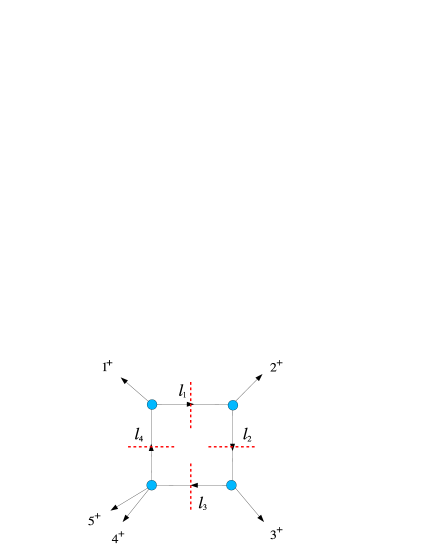
Figure 9: One of the quadruple cuts for the amplitude $1^{+}2^{+}3^{+}4^{+}5^{+}$.

Here we will find that we can reproduce the full amplitude using only quadruple cuts in $4-2\epsilon$ dimensions.

Let us start by considering the diagram in Figure 9, which represents the quadruple cut where gluons $4$ and $5$ enter the same tree amplitude. The momentum constraints on this quadruple cut are given by

$$l_{1}^{2}\,=\,l_{2}^{2}\,=\,l_{3}^{2}\,=\,l_{4}^{2}\,=\,\mu^{2}\ ,$$

$$l_{1}\,=\,l_{4}-k_{1}\ ,\ l_{2}\,=\,l_{1}-k_{2}\ ,\ l_{3}\,=\,l_{2}-k_{3}\ ,\ l_{4}\,=\,l_{3}-k_{4}-k_{5}\ .$$ (4.6)

It will prove convenient to solve for the momentum $l_{3}$, which we expand in the basis of vectors $k_{1},k_{2},k_{3}$ and $K$, where $K$ is defined in (3.23). One finds that the solution of (4) is given by

$$l_{3}\ =\ ak_{1}\,+\,bk_{2}\,+\,ck_{3}\,+\,dK\ ,$$ (4.7)

with

$$a\ =\ \frac{t}{2u}\ ,\ b\ =\ -\frac{1}{2}\ ,\ c\ =\ -1-\frac{s}{2u}\ ,$$ (4.8)

$$d\ =\ \pm\sqrt{-{st+4\mu^{2}u\over stu^{2}}}\ ,$$

where the kinematical invariants $s$, $t$, $u$ are again defined by (3.26), but now $s+t+u=(k_{4}+k_{5})^{2}$.

Considering the diagram in Figure 9, the product of tree-level amplitudes entering the quadruple cut can be written as

$$\frac{\langle q_{1}|l_{1}|1]}{\langle q_{1}1\rangle}\ \frac{\langle q_{2}|l_{2}|2]}{\langle q_{2}2\rangle}\ \frac{\langle q_{3}|l_{3}|3]}{\langle q_{3}3\rangle}\ \frac{\mu^{2}\,[45]}{\langle 45\rangle\,[(l_{3}-k_{4})^{2}-\mu^{2}]}\ \ .$$ (4.9)

Using (3.10), and choosing $q_{3}\!=\!2$, (4.9) can be recast as

$$- \mu^{4}\,{[12]\over\langle 12\rangle}{[45]\over\langle 45\rangle}{1\over\langle 23\rangle}\,{\langle 2|l_{3}|3]\over(l_{3}-k_{4})^{2}-\mu^{2}}\ =\ {\mu^{4}\over\langle 12\rangle\langle 23\rangle\langle 34\rangle\langle 45\rangle\langle 51\rangle}{{\rm Tr_{-}}(5123l_{3}4)\over(l_{3}-k_{4})^{2}-\mu^{2}}$$ (4.10)

$$= -{\mu^{4}\over\langle 12\rangle\langle 23\rangle\langle 34\rangle\langle 45\rangle\langle 51\rangle}{{\rm Tr_{+}}(123l_{3}43)\,+\,{\rm Tr_{+}}(123l_{3}42)\over(l_{3}-k_{4})^{2}-\mu^{2}}\ .$$

Using momentum conservation, and

$${\rm Tr_{+}}(abcd)\ =\ 2\Big{[}(ab)(cd)\,-\,(ac)(bd)\,+\,(ad)(bc)\,+\,i\epsilon(abcd)\Big{]}\ ,$$ (4.11)

it is easy to see that

$${{\rm Tr_{+}}(123l_{3}43)\,+\,{\rm Tr_{+}}(123l_{3}42)\over(l_{3}\cdot k_{4})}\ =\ 4(12)(23)\,-\,4i{(34)\,\epsilon(12l_{3}3)\ -\ (12)\,\epsilon(234l_{3})\over(l_{3}\cdot k_{4})}\ .$$ (4.12)

We set

$$V(l_{3})\ =\ i\epsilon(12l_{3}3)(3\cdot 4)\,-\,i\epsilon(234l_{3})(1\cdot 2)\ .$$ (4.13)

Now we wish to sum the expression (4.10) over the solutions (4.8), including a factor of $1/2$. Writing these solutions as $l_{3}^{\pm}=x\pm y$, where $y$ contains the term involving the momentum $K$, it is straightforward to show that

$$\frac{1}{2}\sum_{l_{3}^{\pm}}{{\rm Tr_{+}}(123l_{3}43)\,+\,{\rm Tr_{+}}(123l_{3}42)\over(l_{3}\cdot k_{4})}\ =\ 4\,(1\cdot 2)(2\cdot 3)\,-\,4{V(x)(x\cdot 4)\,-\,V(y)(y\cdot 4)\over(x\cdot 4)^{2}-(y\cdot 4)^{2}}\ ,$$ (4.14)

and

$${V(x)(x\cdot 4)\,-\,V(y)(y\cdot 4)\over(x\cdot 4)^{2}-(y\cdot 4)^{2}}\ =\ -{i\over 2}\mu^{2}\epsilon(1234)\,\bigg{[}\frac{1}{(l_{3}^{+}\cdot 4)}\,+\,\frac{1}{(l_{3}^{-}\cdot 4)}\bigg{]}\ .$$ (4.15)

Summarising, we have found that

$$\frac{1}{2}\sum_{l_{3}^{\pm}}{{\rm Tr_{+}}(123l_{3}43)\,+\,{\rm Tr_{+}}(123l_{3}42)\over(l_{3}\cdot k_{4})}\ =\ 4\,(1\cdot 2)(2\cdot 3)\,+\,2i\mu^{2}\epsilon(1234)\,\bigg{[}\frac{1}{(l_{3}^{+}\cdot 4)}\,+\,\frac{1}{(l_{3}^{-}\cdot 4)}\bigg{]}$$

$$\qquad\qquad\qquad\quad=\ s_{12}\,s_{23}\,-\,4i\mu^{2}\epsilon(1234)\,\bigg{[}\frac{1}{(l_{3}^{+}-k_{4})^{2}-\mu^{2}}\,+\,\frac{1}{(l_{3}^{-}-k_{4})^{2}-\mu^{2}}\bigg{]}\ .$$ (4.16)

From (4.10), we see that the full amplitude in the quadruple cut is obtained by multiplying (4.16) by $-\mu^{4}/C_{5}$. Next, we lift the cut integral to a full Feynman integral, and get

$$-\,2{\mu^{4}\over C_{5}}\bigg{[}s_{12}\,s_{23}\,-\,4i\mu^{2}\epsilon(1234)\,\bigg{(}\frac{1}{(l_{3}^{+}-k_{4})^{2}-\mu^{2}}\,+\,\frac{1}{(l_{3}^{-}-k_{4})^{2}-\mu^{2}}\bigg{)}\biggr{]}\ \longrightarrow$$

$$\ \ \ \ \qquad-{i\over C_{5}(4\pi)^{2-\epsilon}}\,\biggl{[}I_{4}^{(5),4-2\epsilon}[\mu^{4}]\,s_{12}\,s_{23}\,+\,8iI_{5}^{4-2\epsilon}[\mu^{6}]\,\epsilon(1234)\biggr{]}\$$

$$\qquad\ =\ {i\over C_{5}}{\epsilon(1-\epsilon)\over(4\pi)^{2-\epsilon}}\,\biggl{[}s_{12}\,s_{23}\,I_{4}^{(5),8-2\epsilon}\,+\,4i\,(4-2\epsilon)\,\epsilon(1234)I_{5}^{10-2\epsilon}\biggr{]}\ ,$$ (4.17)

where the factor of $2$ in the first line of (4.17) comes from adding, as usual, the two possible quadruple cuts of the amplitude (which are equal, since they are obtained one from the other by simply flipping all the internal “scalar helicities”).

Let us now discuss the result we have found. The first term in the last line of (4.17) gives the $s_{12}s_{23}$ term in (4.4). The other quadruple cut diagrams, which come from cyclic relabelling of the external legs, will similarly generate the other $\epsilon(1234)$-independent terms in (4.4). Finally, the $\epsilon(1234)$ term in (4.17) – a pentagon integral term – matches the $\epsilon(1234)$ term in (4.4).

Thus we have shown that the five gluon amplitude $+$$+$$+$$+$$+$ may be reconstructed directly using quadruple cuts in $4-2\epsilon$ dimensions.

References

• [1] E. Witten, Perturbative gauge theory as a string theory in twistor space, Commun. Math. Phys.  252, 189 (2004), hep-th/0312171.
• [2] R. Britto, F. Cachazo and B. Feng, New recursion relations for tree amplitudes of gluons, Nucl. Phys. B 715, 499 (2005) hep-th/0412308.
• [3] R. Britto, F. Cachazo, B. Feng and E. Witten, Direct proof of tree-level recursion relation in Yang-Mills theory, hep-th/0501052.
• [4] L. D. Landau, On Analytic Properties Of Vertex Parts In Quantum Field Theory, Nucl. Phys.  13 (1959) 181.
• [5] R. E. Cutkosky, Singularities And Discontinuities Of Feynman Amplitudes, J. Math. Phys.  1 (1960) 429.
• [6] R. J. Eden, P. V. Landshoff, D. I. Olive and J. C. Polkinghorne, The Analytic S-Matrix, Cambridge University Press, 1966.
• [7] J. Bedford, A. Brandhuber, B. Spence and G. Travaglini, A recursion relation for gravity amplitudes, Nucl. Phys. B (in press), hep-th/0502146.
• [8] F. Cachazo and P. Svrcek, Tree level recursion relations in general relativity, hep-th/0502160.
• [9] Z. Bern, L. J. Dixon and D. A. Kosower, On-shell recurrence relations for one-loop QCD amplitudes, hep-th/0501240.
• [10] Z. Bern, L. J. Dixon and D. A. Kosower, The last of the finite loop amplitudes in QCD, hep-ph/0505055.
• [11] S. D. Badger, E. W. N. Glover, V. V. Khoze and P. Svrček, Recursion relations for gauge theory amplitudes with massive particles, hep-th/0504159.
• [12] Z. Bern, L. J. Dixon, D. C. Dunbar and D. A. Kosower, One loop n point gauge theory amplitudes, unitarity and collinear limits, Nucl. Phys. B 425 (1994) 217, hep-ph/9403226.
• [13] Z. Bern, L. J. Dixon, D. C. Dunbar and D. A. Kosower, Fusing gauge theory tree amplitudes into loop amplitudes, Nucl. Phys. B 435 (1995) 59, hep-ph/9409265.
• [14] C. Anastasiou, Z. Bern, L. J. Dixon and D. A. Kosower, Planar amplitudes in maximally supersymmetric Yang-Mills theory, Phys. Rev. Lett.  91, 251602 (2003) hep-th/0309040.
• [15] C. Anastasiou, Z. Bern, L. J. Dixon, and D. A. Kosower, Cross-order relations in N = 4 supersymmetric gauge theories, hep-th/0402053.
• [16] Z. Bern, L. J. Dixon and V. A. Smirnov, Iteration of planar amplitudes in maximally supersymmetric Yang-Mills theory at three loops and beyond, hep-th/0505205.
• [17] F. Cachazo, P. Svrček and E. Witten, MHV vertices and tree amplitudes in gauge theory, JHEP 0409, 006 (2004) hep-th/0403047.
• [18] C. J. Zhu, The googly amplitudes in gauge theory, JHEP 0404, 032 (2004), hep-th/0403115.
• [19] G. Georgiou and V. V. Khoze, Tree amplitudes in gauge theory as scalar MHV diagrams, JHEP 0405, 070 (2004), hep-th/0404072.
• [20] J. B. Wu and C. J. Zhu, MHV vertices and scattering amplitudes in gauge theory, JHEP 0407, 032 (2004) hep-th/0406085.
• [21] J. B. Wu and C. J. Zhu, MHV vertices and fermionic scattering amplitudes in gauge theory with quarks and gluinos, JHEP 0409, 063 (2004) hep-th/0406146.
• [22] G. Georgiou, E. W. N. Glover and V. V. Khoze, Non-MHV tree amplitudes in gauge theory, JHEP 0407, 048 (2004) hep-th/0407027.
• [23] L. J. Dixon, E. W. N. Glover and V. V. Khoze, MHV rules for Higgs plus multi-gluon amplitudes, JHEP 0412 (2004) 015, hep-th/0411092.
• [24] Z. Bern, D. Forde, D. A. Kosower and P. Mastrolia, Twistor-inspired construction of electroweak vector boson currents, hep-ph/0412167.
• [25] N. Berkovits and E. Witten, Conformal supergravity in twistor-string theory, JHEP 0408, 009 (2004), hep-th/0406051.
• [26] A. Brandhuber, B. Spence and G. Travaglini, One-loop gauge theory amplitudes in N = 4 super Yang-Mills from MHV vertices, Nucl. Phys. B 706, 150 (2005), hep-th/0407214.
• [27] F. Cachazo, P. Svrcek and E. Witten, Twistor space structure of one-loop amplitudes in gauge theory, JHEP 0410 (2004) 074, hep-th/0406177.
• [28] F. Cachazo, P. Svrcek and E. Witten, Gauge theory amplitudes in twistor space and holomorphic anomaly, JHEP 0410 (2004) 077, hep-th/0409245.
• [29] I. Bena, Z. Bern, D. A. Kosower and R. Roiban, Loops in twistor space, hep-th/0410054.
• [30] F. Cachazo, Holomorphic anomaly of unitarity cuts and one-loop gauge theory amplitudes, hep-th/0410077.
• [31] R. Britto, F. Cachazo and B. Feng, Computing one-loop amplitudes from the holomorphic anomaly of unitarity cuts, Phys. Rev. D 71 (2005) 025012, hep-th/0410179.
• [32] Z. Bern, V. Del Duca, L. J. Dixon and D. A. Kosower, All non-maximally-helicity-violating one-loop seven-gluon amplitudes in N = 4 super-Yang-Mills theory, Phys. Rev. D 71 (2005) 045006, hep-th/0410224.
• [33] S. J. Bidder, N. E. J. Bjerrum-Bohr, L. J. Dixon and D. C. Dunbar, N = 1 supersymmetric one-loop amplitudes and the holomorphic anomaly of unitarity cuts, Phys. Lett. B 606 (2005) 189, hep-th/0410296.
• [34] C. Quigley and M. Rozali, One-loop MHV amplitudes in supersymmetric gauge theories, JHEP 0501 (2005) 053 hep-th/0410278.
• [35] J. Bedford, A. Brandhuber, B. Spence and G. Travaglini, A twistor approach to one-loop amplitudes in N = 1 supersymmetric Yang-Mills theory, Nucl. Phys. B 706, 100 (2005), hep-th/0410280;
• [36] J. Bedford, A. Brandhuber, B. Spence and G. Travaglini, Non-supersymmetric loop amplitudes and MHV vertices, Nucl. Phys. B 712, 59 (2005) hep-th/0412108.
• [37] W. L. van Neerven, Dimensional Regularization Of Mass And Infrared Singularities In Two Loop On-Shell Vertex Functions, Nucl. Phys. B 268 (1986) 453.
• [38] Z. Bern and A. G. Morgan, Massive Loop Amplitudes from Unitarity, Nucl. Phys. B 467 (1996) 479, hep-ph/9511336.
• [39] Z. Bern, L. J. Dixon, D. C. Dunbar and D. A. Kosower, One-loop self-dual and N = 4 super Yang-Mills, Phys. Lett. B 394 (1997) 105, hep-th/9611127.
• [40] Z. Bern, L. J. Dixon and D. A. Kosower, One-loop amplitudes for e+ e- to four partons, Nucl. Phys. B 513 (1998) 3, hep-ph/9708239.
• [41] Z. Bern, L. J. Dixon and D. A. Kosower, A two-loop four-gluon helicity amplitude in QCD, JHEP 0001 (2000) 027, hep-ph/0001001.
• [42] Z. Bern, L. J. Dixon and D. A. Kosower, Two-loop g $\to$ g g splitting amplitudes in QCD, JHEP 0408 (2004) 012, hep-ph/0404293.
• [43] R. Britto, F. Cachazo and B. Feng, Generalized unitarity and one-loop amplitudes in N = 4 super-Yang-Mills, hep-th/0412103.
• [44] Z. Bern, L. J. Dixon and D. A. Kosower, All next-to-maximally helicity-violating one-loop gluon amplitudes in N = 4 super-Yang-Mills theory, hep-th/0412210.
• [45] S. J. Bidder, N. E. J. Bjerrum-Bohr, D. C. Dunbar and W. B. Perkins, One-loop gluon scattering amplitudes in theories with $N<4$ supersymmetries, Phys. Lett. B 612 (2005) 75, hep-th/0502028.
• [46] R. Britto, E. Buchbinder, F. Cachazo and B. Feng, One-loop amplitudes of gluons in SQCD, hep-ph/0503132.
• [47] Z. Bern and D. A. Kosower, The Computation of loop amplitudes in gauge theories, Nucl. Phys. B 379 (1992) 451.
• [48] Z. Bern, L. J. Dixon and D. A. Kosower, New QCD results from string theory, hep-th/9311026.
• [49] Z. Bern, G. Chalmers, L. J. Dixon and D. A. Kosower, One loop N gluon amplitudes with maximal helicity violation via collinear limits, Phys. Rev. Lett.  72 (1994) 2134, hep-ph/9312333.
• [50] Z. Bern, L. J. Dixon and D. A. Kosower, One-Loop Corrections to Five-Gluon amplitudes, Phys. Rev. Lett. 70 (1993) 2677-2680, hep-ph/9302280.
• [51] Z. Bern and G. Chalmers, Factorization in One-Loop Gauge Theory, Nucl. Phys. B 447 (1995) 465-518, hep-ph/9503236.