Bubbling Orientifolds

Abstract:

We investigate a class of ${\frac{1}{2}}$-BPS bubbling geometries associated to orientifolds of type IIB string theory and thereby to excited states of the $SO(N)/Sp(N)$ ${\cal N}=4$ supersymmetric Yang-Mills theory. The geometries are in correspondence with free fermions moving in a harmonic oscillator potential on the half-line. Branes wrapped on torsion cycles of these geometries are identified in the fermi fluid description. Besides being of intrinsic interest, these solutions may also occur as local geometries in flux compactifications where orientifold planes are present to ensure global charge cancellation. We comment on the extension of this procedure to M-theory orientifolds.

1 Introduction

The recent discovery [1] of an infinite set of ${\frac{1}{2}}$-BPS geometries of type IIB supergravity is of great interest. This discovery provides a correspondence between semiclassical states of the matrix harmonic oscillator and ${\frac{1}{2}}$-BPS geometries, in which the ground state of the matrix model (equivalent to a fermi fluid in a harmonic oscillator potential) corresponds to the well-known $AdS_{5}\times S^{5}$ geometry. Also, the $pp$-wave geometry emerges in the limit of relativistic fermions. A similar construction also exists for ${\frac{1}{2}}$-BPS backgrounds of 11-dimensional supergravity.

These geometries can have various interpretations, as D-branes and/or giant gravitons/dual giant gravitons, depending on the typical sizes of various regions. Their relation to a fermi fluid profile arises from the fact that one can pick an arbitrary shading of the complex plane into black and white regions (denoting occupied/unoccupied regions of fermion phase space) and input this data to construct a ${\frac{1}{2}}$-BPS supergravity solution with fluxes. The matrix oscillator in turn arises[2, 3] (see also Ref.[4]) in the ${\cal N}=4$ supersymmetric Yang-Mills theory on a D3-brane wrapped on $S^{3}$, which has a coupling of the form $\int\sqrt{g}R\,\phi_{i}^{2}$ for each complex scalar field $\phi_{i}$ of the ${\cal N}=4$ supermultiplet.

This discovery provides a somewhat new insight into holography. Not only do ${\frac{1}{2}}$-BPS operators of the ${\cal N}=4$ SYM theory correspond to excited states of supergravity on $AdS_{5}\times S^{5}$, as was already known for a long time[5, 6, 7], but they can also be identified with entirely new ${\frac{1}{2}}$-BPS geometries. These geometries can possess quite different topologies and one can understand topology change as the process of fermi fluid profiles merging and separating[1, 11]. The phase space of the fermi fluid is realised on 2 of the 9 space dimensions of 10-dimensional type IIB supergravity. This implies that the gravity configuration space is partly noncommutative, explanations of which have been proposed in Refs.[12, 13] (related observations can be found in Ref.[14]).

In the present work we would like to investigate the bubbling geometry construction in the presence of an intrinsically stringy effect, namely the orientifold plane. This ubiquitous object has led to important insights in the past[15, 16]. In gauge theory terms it can be used to modify the gauge group from $SU(N)$ to $SO(2N),SO(2N+1)$ or $Sp(2N)$ without breaking any supersymmetry. From the gravity point of view, parallel orientifold planes and D-branes break the same supersymmetries, so it is not surprising that we will find bubbling orientifolded geometries that are ${\frac{1}{2}}$-BPS. This adds a nontrivial class of new geometries to the ones proposed in Ref.[1]. The “ground state” geometry in this case is $AdS_{5}\times RP^{5}$, an example studied in depth in Ref.[17].

Besides providing more general examples of “bubbling geometries”, the introduction of orientifold planes in this context is likely to be of practical interest. For compactifications of string theory with space-filling branes and/or fluxes, it is well-known that the absence of tadpoles requires space-filling orientifolds. In Ref.[18], it has been noted that the $T^{6}/Z_{2}\times R^{3,1}$ orientifold compactification has precisely $AdS_{5}\times RP^{5}$ as the local geometry around the space-filling D3-branes if they are brought near an orientifold. So besides representing a ${\frac{1}{2}}$-BPS geometry by itself, $AdS_{5}\times RP^{5}$ can also be thought of as a possible local geometry for a ${\frac{1}{2}}$-BPS compactification. This suggests a more general class of ${\frac{1}{2}}$-BPS compactifications (involving both branes and fluxes) for which the spacetimes discussed in the present paper could appear as local geometries.

In what follows we first briefly review bubbling geometries as well as orientifold 3-planes. Following this we describe the bubbling orientifold geometries and their realisation in terms of free fermions on a phase space that is the upper half-plane. We will see that the orientifold plane can be interpreted as the wall which truncates a regular harmonic oscillator potential to a “half-oscillator”, a familiar problem in quantum mechanics. We comment on the topology and other characteristics of the most general bubbling solutions, including discrete torsion and the possibility of two different types of topology change. Finally we briefly examine the analogue solutions in $M$-theory. In the Appendix, we collect some useful facts about random matrices in a harmonic oscillator potential, for the cases when the matrices are in the Lie algebra of $SO(2N+1),Sp(2N),SO(2N)$. These matrix models compute the ${\frac{1}{2}}$-BPS states of ${\cal N}=4$ super-Yang-Mills theory with the corresponding gauge groups.

2 Bubbling Geometries: A Brief Review

The type IIB ${\frac{1}{2}}$-BPS bubbling geometries of Ref.[1] can be summarised in a family of classical solutions of type IIB supergravity given in terms of a single function $z(y;x_{1},x_{2})$. The metrics contain two 3-spheres $S^{3}$ and ${\tilde{S}}^{3}$ and are given by:

$$ds^{2} = -\left[{y^{2}\over\frac{1}{4}-z^{2}}\right]^{\frac{1}{2}}\,(dt+V_{i}\,dx_{i})^{2}+\left[{\frac{1}{4}-z^{2}\over y^{2}}\right]^{\frac{1}{2}}\,(dy^{2}+dx_{i}\,dx_{i})$$ (1)

$$+\left[y^{2}\,{\frac{1}{2}+z\over\frac{1}{2}-z}\right]^{\frac{1}{2}}\,d\Omega_{3}^{2}+\left[y^{2}\,{\frac{1}{2}-z\over\frac{1}{2}+z}\right]^{\frac{1}{2}}\,d{\tilde{\Omega}}_{3}^{2}$$

Additionally the solution has suitable 5-form fluxes. The function $z=z(y;x_{1},x_{2})$ satisfies:

$$(\partial_{y}^{2}+\partial_{i}\partial_{i})z-{1\over y}\,\partial_{y}z=0$$ (2)

and $V_{i}$ is a vector field determined in terms of $z$ via:

$$y\,\partial_{y}V_{i}=\epsilon_{ij}\,\partial_{j}z,\quad y\,\partial_{[i}V_{j]}=\epsilon_{ij}\,\partial_{y}z$$ (3)

¿From the metric, it is clear that the range of the $y$ coordinate is restricted to $y\geq 0$. Also as $y\to 0$, smoothness of the metric requires $z\to\pm\frac{1}{2}$ with $y/\sqrt{\frac{1}{2}\mp z}$ fixed. Then if $z\to+\frac{1}{2}$, the 3-sphere ${\tilde{S}}^{3}$ with metric proportional to $d{\tilde{\Omega}}_{3}^{2}$ shrinks to zero size, while the other 3-sphere $S^{3}$ with metric $d\Omega_{3}^{2}$ remains finite. When $z\to-\frac{1}{2}$ the reverse is true, and it is $S^{3}$ that shrinks to zero size. More details are given in Ref.[1]. The geometries are parametrised by drawing smooth contours in the $x_{1},x_{2}$ plane which demarcate regions of $z=-\frac{1}{2}$ (black) from regions of $z=+\frac{1}{2}$ (white). In turn, these regions can be interpreted as semiclassical phase-space profiles of a fermi fluid where the black regions are occupied and the white regions are unoccupied. The constant phase-space densities of these droplets map to constant densities in the $x_{1},x_{2}$ plane. This follows from the fact that the flux through a sphere formed by drawing a surface ending on a black/white region can be converted to an integral of a constant flux density over the region.

Fermi fluid profiles consisting of a black disc with a circular boundary correspond to the $AdS_{5}\times S^{5}$ solution. Deformations of this by adding/removing thin concentric shells correspond to giant gravitons or dual giant gravitons in this spacetime. But the most generic geometry can have very little to do with $AdS_{5}\times S^{5}$ and may contain, for example, an arbitrary number of $S^{5}$ factors.

The bubbling construction can be extended to ${\frac{1}{2}}$-BPS solutions of 11-dimensional supergravity. In this case one finds metrics parametrised in terms of a function $D(y;x_{1},x_{2})$. In what follows, we denote $\partial_{y}D$ by $D^{\prime}$. These metrics contain a five-sphere $S^{5}$ and a two-sphere ${\tilde{S}}^{2}$, and are given by:

$$ds^{2} = -4\left[{y\over D^{\prime}(1-yD^{\prime})^{2}}\right]^{1\over 3}(dt+V_{i}\,dx^{i})^{2}+\left[{{D^{\prime}}^{2}(1-yD^{\prime})\over y^{2}}\right]^{1\over 3}\Big{(}dy^{2}+e^{D}(dx_{1}^{2}+dx_{2}^{2})\Big{)}$$ (4)

$$+4\left[{y(1-yD^{\prime})\over D^{\prime}}\right]^{1\over 3}d\Omega_{5}^{2}+\left[{y^{2}D^{\prime}\over(1-yD^{\prime})}\right]^{2\over 3}d{\tilde{\Omega}}_{2}^{2}$$

along with a suitable 4-form flux. The function $D(y;x_{1},x_{2})$ satisfies the three-dimensional Toda equation:

$$\partial_{i}\partial_{i}D+\partial_{y}^{2}e^{D}=0$$ (5)

and the vector field is determined in terms of $D$ by:

$$V_{i}=\frac{1}{2}\epsilon_{ij}\partial_{j}D$$ (6)

In this class of metrics too, the range of the coordinate $y$ is restricted to $y\geq 0$ and as $y\to 0$, the function $D$ must obey one of two boundary conditions. One possibility is $D^{\prime}\sim y$ while the other is $D^{\prime}\sim y^{-1}$. More precisely we have:

(i) $$D~{}\to~{}y^{2}+g(x_{1},x_{2})$$

(ii) $$D~{}\to~{}\log y+h(x_{1},x_{2})$$ (7)

where $g,h$ are functions of $(x_{1},x_{2})$ satisfying the two-dimensional Liouville equation:

$$\partial_{i}\partial_{i}\,g(x_{1},x_{2})+e^{g(x_{1},x_{2})}=0$$ (8)

and similarly for $h(x_{1},x_{2})$.

In case (i), keeping $D$ finite in the limit, it is evident from the metric Eq. (4) that ${\tilde{S}}^{2}$ shrinks to zero size while $S^{5}$ remains finite. In case (ii) we keep $D^{\prime}-y^{-1}$ finite in the limit and find that $S^{5}$ shrinks with ${\tilde{S}}^{2}$ remaining finite. Thus again the $x_{1},x_{2}$ plane is divided into two types of regions, which can be associated to fermi fluid droplets. There is an important subtlety[1]: the density of fermions in a droplet is not constant, unlike in the type IIB case. In fact the densities of the droplets are

(i) $$\rho(x_{1},x_{2})=2\,e^{g(x_{1},x_{2})}$$

(ii) $$\rho(x_{1},x_{2})=2\,e^{h(x_{1},x_{2})}.$$ (9)

However, as argued by the authors of Ref.[1], two droplets related by a conformal mapping of the plane give rise to the same ${\frac{1}{2}}$-BPS solution. Therefore the topology of the bubbles in the $(x_{1},x_{2})$ plane is expected to be the same as that in the fermion phase space. In particular, they demonstrate that the M-theory pp-wave is given by one of the two boundary conditions for $x_{2}<0$ and the other one for $x_{2}>0$, just as one would expect from the correspondence of this system with the relativistic limit of free fermions.

3 The $AdS_{5}\times RP^{5}$ Orientifold

In Ref.[1], ${\frac{1}{2}}$-BPS excitations of a ground state geometry corresponding to $AdS_{5}\times S^{5}$ in type IIB string theory were considered, and the full back reaction on the geometry was determined. We will instead be interested in an $AdS_{5}\times RP^{5}$ ground state, arising from a $Z_{2}$ orientifold projection of the $S^{5}$, as considered by Witten[17].

Introducing an orientifold plane changes the gauge group on a stack of D-branes to $SO(2N)$, $SO(2N+1)$ or $Sp(2N)$, instead of previously $SU(N)$. The orientifolded theory has no fixed points on the $S^{5}$, so there is no open string sector. Being an orientifold, traversing a non-contractible loop flips the orientation of the world-sheet (or any embedded orientable manifold). This means that there is also no “winding sector”. The spectrum therefore consists only of those $AdS_{5}\times S^{5}$ states which are invariant under the orientifold projection, at least for weak coupling.

The topology of the 2-form fields $B_{NS\,NS}$ and $B_{RR}$ is in general non-trivial, in the sense that the field strength $H=dB$ belongs to some equivalence class of the cohomology group $H^{3}(AdS_{5}\times RP^{5},\tilde{Z})=H^{3}(RP^{5},\tilde{Z})=Z_{2}$, where $\tilde{Z}$ denotes twisted coefficients, i.e. coefficients flipping sign along a non-contractible loop. To preserve supersymmetry, it is necessary to choose $H=0$. We have already said that traversing a non-contractible loop flips the orientation of the world-sheet $\Sigma$. Again using twisted coefficients, this means that the homology is $\Sigma\in H_{2}(RP^{5},\tilde{Z})=Z_{2}$, and we may represent the non-trivial element by $RP^{2}$. Consequently, for non-trivial choice of discrete torsion for the field strength, the contribution to the path integral is $e^{i\int_{\Sigma}B_{NS\,NS}}=(-1)^{s}$, where $s$ is the number of $RP^{2}$’s making up the world-sheet. Trivial choice of torsion always contributes a factor of unity.

There will be four distinct combinations of discrete torsion which can be labelled by

$$\theta_{NS\,NS} = {1\over 2\pi}\int_{\Sigma}B_{NS\,NS}$$

$$\theta_{RR} = {1\over 2\pi}\int_{\Sigma}B_{RR},$$ (10)

so that $\theta_{NS\,NS}$ and $\theta_{RR}$ can independently take the values $0,\frac{1}{2}$. The $(0,0)$ theory can be shown to be $SL(2,Z)$ invariant. The Montonen-Olive duality of such a theory identifies it as $SO(2N)$. Turning on $\theta_{NS\,NS}=\frac{1}{2}$ will change the gauge group to $Sp(2N)$, which can be seen in the following way. Feynman diagrams of $Sp(2N)$ are obtained from those of $SO(2N)$ by sending $N\rightarrow-N$. Since the contribution of a generic diagram goes as $N^{2-2g-s}$, where $g$ is the genus and $s$ is the number of glued copies of $RP^{2}$, we conclude that each $RP^{2}$ contributes a factor $-1$. By definition of the discrete torsion, this is precisely the effect of turning on $\theta_{NS\,NS}$. This argument therefore indicates that turning on $\theta_{NS\,NS}=\frac{1}{2}$ (with $\theta_{RR}=0$ or $\frac{1}{2}$) is equivalent to changing the gauge group from $SO(2N)$ (or $SO(2N+1)$) to $Sp(2N)$. The only combination of discrete torsions which is left is $(\theta_{NS\,NS},\theta_{RR})=(0,\frac{1}{2})$, which can be identified with the “remaining” gauge group, $SO(2N+1)$.

Interestingly, the torsion need not be constant all over the manifold. To explain this, some background on 3-branes in this geometry is required. In addition to the ordinary $D3$ brane, the $AdS_{5}\times RP^{5}$ theory also contains 3-branes resulting from wrapping a 5-brane on an $RP^{2}$ submanifold of the $RP^{5}$. Any 3-brane is localised in one spatial direction on the $AdS_{5}$ space. The $D3$ brane is a source of 5-form flux, so the brane will act as a domain wall, separating $SU(N)$ and $SU(N+1)$ gauge theories on the boundary. On the orientifold, the flux $N$ through $S^{5}$, which covers the $RP^{2}$ twice, will instead shift by two units. Therefore, the gauge group will shift between $SO(2N)$ and $SO(2N+2)$ or between $Sp(2N)$ and $Sp(2N+2)$. But crossing a 3-brane made by wrapping a D5 or NS5-brane on $RP^{2}$ also makes the $\theta$ angle jump. This is because the wrapped 5-brane also acts as a source for the field $H=dB$. A wrapped $D5$ brane sources RR-form flux, and so makes $\theta_{RR}$ jump. Similarly, a wrapped $NS5$ brane has NS-flux on it, making $\theta_{NS\,NS}$ jump upon crossing it. We will discuss how these features relate to the LLM description in section 5.2.

In general, branes characterized by untwisted or twisted charges can only be wrapped on non-trivial cycles with untwisted or twisted coefficients, respectively. In addition, topological considerations may restrict the allowed values of the discrete torsions. In spite of these restrictions, the $RP^{5}$ geometry still introduces new types of objects, as compared to the unorientifolded theory, such as fat strings and Pfaffian particles (on the gauge theory side). They can be constructed by wrapping branes on non-trivial cycles of the $RP^{5}$ which lack any counterpart in the $S^{5}$ theory. We refer to Ref.[17] for details.

Here, we will content ourselves by illustrating some of the general features involved by discussing some properties of the baryon vertex of $SU(N)$ gauge theory, which does exist both before and after the projection to the $RP^{5}$ geometry. In the unprojected case, the only non-trivial cycle is the full $S^{5}$ itself. The baryon vertex is constructed by wrapping a $D5$ brane on this $S^{5}$. Strings connect it to $N$ external quarks. Quarks are particles in the fundamental representation of the gauge group. The combination is fermionic, since it is made gauge invariant by contracting the colour wave functions using an antisymmetric tensor of order $N$.

That this makes sense from the gravity point of view can be seen as follows. There is a coupling $\frac{1}{2\pi}\int_{S^{5}\times R}a\wedge F_{5}$ on the world-volume of the $D5$ brane. As always, $\int_{S^{5}}F_{5}=2\pi N$, so the charge corresponding to the $U(1)$ gauge field $a$ gets a contribution of $N$ units due to the $D5$ brane. Similarly, each of the $N$ fundamental strings ending on the $D5$ contributes by $-1$, making the total charge vanish, as required.

The other ends of the strings connect to quarks at the boundary, modelled by attaching their endpoints to a large $D3$ brane whose spatial world-volume is of the topology $S^{3}\times P$, where $P$ is a point on the $S^{5}$. Placing the wrapped $D5$ at the point $Q$ in $AdS_{5}$ and considering the “linking” numbers between the manifolds $S^{3}\times P$ and $Q\times S^{5}$, there will be a change of sign associated with interchanging two strings, confirming that the strings are fermionic.

In the projected theory, topological restrictions allow the $D5$ to wrap the $RP^{5}$ an even number of times only. Hence, the baryon vertex only couples to an even number of quarks on the orientifold.

4 Bubbling Orientifolds and Fermi Fluids

In the previous section we have seen that the spacetime $AdS_{5}\times S^{5}$ admits an involution that reflects all the directions of the 5-sphere and converts it into the real projective space $RP^{5}$. The dual gauge theory is the ${\cal N}=4$ super-Yang-Mills theory on a set of D3-branes parallel to an orientifold 3-plane. The gauge group can be $SO(2N)$, $SO(2N+1)$ or $Sp(2N)$ depending on the precise type of O3-plane. In keeping with the bubbling geometry idea, we expect that there should be an infinite set of ${\frac{1}{2}}$-BPS bubbling geometries that correspond to the excited states of this gauge theory.

To find these, we need to understand how the fermi fluid profile that corresponds to $AdS_{5}\times S^{5}$ is affected by the orientifolding. This profile is a circle of radius $r_{0}=R_{AdS}^{2}$ in the fermion phase space. In the geometry this space is realised as the $x_{1}-x_{2}$ plane. Now $AdS_{5}\times S^{5}$ is parametrised as:

$$(ds)^{2}=r_{0}\left(-\cosh^{2}\rho\,dt^{2}+d\rho^{2}+\sinh^{2}\rho\,d\Omega_{3}^{2}+d\theta^{2}+\cos^{2}\theta\,d{\tilde{\phi}}^{2}+\sin^{2}\theta\,d{\tilde{\Omega}}_{3}^{2}\right)$$ (11)

with $\theta\in[0,\frac{\pi}{2}],{\tilde{\phi}}\in[0,2\pi]$. In terms of embedding coordinates in an ${\rm I\kern-1.79993ptR}^{6}$, one can write:

$$X_{1} = R\,\cos\gamma\,\sin\alpha\,\sin\theta$$

$$X_{2} = R\,\sin\gamma\,\sin\alpha\,\sin\theta$$

$$X_{3} = R\,\cos\beta\,\cos\alpha\,\sin\theta$$

$$X_{4} = R\,\sin\beta\,\cos\alpha\,\sin\theta$$

$$X_{5} = R\,\cos{\tilde{\phi}}\,\cos\theta$$

$$X_{6} = R\,\sin{\tilde{\phi}}\,\cos\theta$$ (12)

with $\alpha,\theta\in[0,\frac{\pi}{2}]$ and $\beta,\gamma,{\tilde{\phi}}\in[0,2\pi]$. The embedding condition is $\sum_{i}X_{i}^{2}=R^{2}\equiv r_{0}$.

The orientifold action on this ${\rm I\kern-1.79993ptR}^{6}$ is $X_{I}\to-X_{I}$, $I=1,2,\cdots,6$. In terms of the angular variables this amounts to

$$\beta \to \beta+\pi$$

$$\gamma \to \gamma+\pi$$

$${\tilde{\phi}} \to {\tilde{\phi}}+\pi.$$ (13)

Going to the $x_{1}-x_{2}$ plane of the bubbling geometry, we recall that it is described by polar coordinates $(r,\phi)$ where

$$r = r_{0}\,\cosh\rho\,\cos\theta$$

$$\phi = {\tilde{\phi}}+t,$$ (14)

and $\rho,{\tilde{\phi}}$ are the coordinates appearing in Eq.(11) above. Therefore, under the orientifolding operation, the $x_{1}-x_{2}$ plane undergoes the involution $\phi\to\phi+\pi$, which is the same as the reflection $(x_{1},x_{2})\to(-x_{1},-x_{2})$.

The precise picture is a little more complicated because at $y=0$, the full spatial geometry is not really 2-dimensional. In the regions where $z=\pm\frac{1}{2}$ (the white and black regions) the geometry is 5-dimensional, and consists of the $(x_{1},x_{2})$ plane together with one of the 3-spheres $S^{3}$ or ${\tilde{S}}^{3}$, parametrised respectively by $d\Omega_{3}$ or $d{\tilde{\Omega}}_{3}$, while the other 3-sphere has shrunk to zero size. The sphere ${\tilde{S}}^{3}$ lies inside $S^{5}$ (and is parametrised by the angles $\alpha,\beta,\gamma$ in Eq.(12)). Thus it is inverted by the orientifold action, while the other 3-sphere $S^{3}$ that lies in $AdS_{5}$ remains unaffected. Thus, at a generic point of the $(x_{1},x_{2})$ plane, the orientifold involution acts by reflecting $(x_{1},x_{2})$ and simultaneously inverting ${\tilde{S}}^{3}$. In the white regions, where $z=\frac{1}{2}$, the ${\tilde{S}}^{3}$ shrinks to zero size, while in the black regions, where $z=-\frac{1}{2}$, it is $S^{3}$ that shrinks. It follows that in the white regions, the orientifolding operation acts solely by inverting the $(x_{1},x_{2})$ plane and turning it into ${\hbox{\kern 3.00003pt{\cmss I}$\kern-3.99994pt{\rm C}$}}/\mathchoice{\hbox{\cmss Z\kern-3.99994ptZ}}{\hbox{\cmss Z\kern-3.99994ptZ}}{\lower 0.9pt\hbox{\cmsss Z\kern-2.79996ptZ}}{\lower 1.2pt\hbox{\cmsss Z\kern-2.79996ptZ}}_{2}$. The same is true on boundaries between the black and white regions with $z=-\frac{1}{2},z=+\frac{1}{2}$ respectively (where both $S^{3},{\tilde{S}}^{3}$ shrink). In the black region, however, one has to keep in mind that the ${\tilde{S}}^{3}$ above a given point of the $(x_{1},x_{2})$ plane is identified with a reversed ${\tilde{S}}^{3}$ above the diametrically opposite point. Finally, at the origin $x_{1}=x_{2}=0$ which is the fixed point of $\phi\to\phi+\pi$, the ${\tilde{S}}^{3}$ gets an antipodal identification and becomes $RP^{3}$.

The above discussion was based on an involution that is a symmetry of the $AdS_{5}\times S^{5}$ background. Therefore strictly speaking it applies only to the simple fermi fluid profile consisting of a black disc of fixed radius centred at the origin. But now it is clear how to define orientifolding for the most general bubbling geometry: simply consider all fermi fluid profiles whose boundaries are well-defined on ${\hbox{\kern 3.00003pt{\cmss I}$\kern-3.99994pt{\rm C}$}}/\mathchoice{\hbox{\cmss Z\kern-3.99994ptZ}}{\hbox{\cmss Z\kern-3.99994ptZ}}{\lower 0.9pt\hbox{\cmsss Z\kern-2.79996ptZ}}{\lower 1.2pt\hbox{\cmsss Z\kern-2.79996ptZ}}_{2}$. Such boundaries have to be invariant under a rotation by $\pi$ in the $(x_{1},x_{2})$ plane. Alternatively they may be drawn on the fundamental domain of ${\hbox{\kern 3.00003pt{\cmss I}$\kern-3.99994pt{\rm C}$}}/\mathchoice{\hbox{\cmss Z\kern-3.99994ptZ}}{\hbox{\cmss Z\kern-3.99994ptZ}}{\lower 0.9pt\hbox{\cmsss Z\kern-2.79996ptZ}}{\lower 1.2pt\hbox{\cmsss Z\kern-2.79996ptZ}}_{2}$: the upper half-plane with the positive and negative halves of the $x_{1}$ axis identified with each other.

What is the fermi system dual to these spacetimes? For this system, the eigenvalue phase space should be an orbifold ${\hbox{\kern 3.00003pt{\cmss I}$\kern-3.99994pt{\rm C}$}}/\mathchoice{\hbox{\cmss Z\kern-3.99994ptZ}}{\hbox{\cmss Z\kern-3.99994ptZ}}{\lower 0.9pt\hbox{\cmsss Z\kern-2.79996ptZ}}{\lower 1.2pt\hbox{\cmsss Z\kern-2.79996ptZ}}_{2}$. This means the position $x$ of the fermion is strictly positive (recall that the identification between coordinate space and phase space is $(x_{1},x_{2})\to(p,x)$). The identification of the positive and negative momentum axes tells us that at $x=0$ the momentum is instantaneously reversed. This is consistent with the harmonic oscillator being truncated to the “half harmonic oscillator” with an infinite vertical wall at $x=0$, a well-known system in quantum mechanics. Thus we have a (Hermitian) matrix-valued particle, or equivalently fermionic eigenvalues, moving in this potential. The fermionic wave functions are made in the usual way out of one-particle wave functions, the latter now being the parity-odd solutions of the full harmonic oscillator.

¿From the correspondence between states of the matrix harmonic oscillator and ${\frac{1}{2}}$-BPS excitations of ${\cal N}=4$ SYM, we would expect the appropriate matrix model for an orientifolded geometry to be related to ${\cal N}=4$ SYM with gauge group $SO(2N)$. Then, following the arguments of Refs.[2, 3], one should get a usual, not semi-infinite, harmonic oscillator, the only change being that the Hermitian matrix (in the algebra of $SU(N)$) is replaced by an antisymmetric matrix (in the algebra of $SO(2N)$).

This appears to be a different theory, but in fact the two descriptions are equivalent, for the same reason that (in flat space) an orientifold plane projects $SU(N)$ Chan-Paton factors down to the $SO$ or $Sp$ subgroup. Consider the random matrix model for $2N\times 2N$ real antisymmetric matrices $A$ (for simplicity we choose constant matrices) with a potential $V(A)$:

$$Z=\int[dA]e^{-{\bf\,tr\,}V(A)}$$ (15)

This is invariant under the orthogonal transformations, which can be used to reduce the matrix $A$ to the form

$$\Lambda = \pmatrix{\lambda_{1}\pmatrix{0&1\cr-1&0}&0&\cdots&0\cr 0&\lambda_{2}\pmatrix{0&1\cr-1&0}&\cdots&0\cr\cdots&\cdots&\phantom{\pmatrix{0&1\cr-1&0}}&\cdots\cr 0&0&\cdots&\lambda_{N}\pmatrix{0&1\cr-1&0}}$$ (16)

$$= i\sigma_{2}\otimes{\rm diag}(\lambda_{1},\lambda_{2},\ldots,\lambda_{N}).$$

Importantly, all $\lambda_{i}$ are real and can be chosen to be non-negative. For example, in each block, a negative $\lambda_{i}$ can be brought to a positive one by conjugating with $\sigma_{3}\otimes{1\kern-3.20007pt1}$.

The matrix measure

$$[dA]\equiv\prod_{P<Q}dA_{PQ}$$ (17)

can then be shown to reduce to

$$[dA] = \prod_{j<k=1}^{N}(\lambda_{j}^{2}-\lambda_{k}^{2})^{2}\prod_{i=1}^{N}d\lambda_{i}$$ (18)

$$= \prod_{j<k=1}^{N}(\lambda_{j}-\lambda_{k})^{2}\prod_{j<k=1}^{N}(\lambda_{j}+\lambda_{k})^{2}\prod_{i=1}^{N}d\lambda_{i}.$$

The nontrivial measure factor just corresponds to $\sqrt{g}$ for the metric $g_{IJ}$ on the space of deformations, in the coordinates made up of the $\lambda_{i}$ and the orthogonal transformations.

Once we know the metric, we easily derive the kinetic term in the Hamiltonian for this matrix model, which is just the Laplacian on the deformation space,

$$H = \sum_{i}{1\over\sqrt{g}}{\partial\over\partial\lambda_{i}}\sqrt{g}{\partial\over\partial\lambda_{i}}={1\over\prod_{j<k}(\lambda_{j}^{2}-\lambda_{k}^{2})^{2}}\,\sum_{i}{\partial\over\partial\lambda_{i}}\prod_{j<k}(\lambda_{j}^{2}-\lambda_{k}^{2})^{2}\,{\partial\over\partial\lambda_{i}}$$ (19)

$$= {1\over\prod_{j<k}(\lambda_{j}^{2}-\lambda_{k}^{2})}\,\sum_{i}{\partial^{2}\over\partial\lambda_{i}^{2}}\prod_{j<k}(\lambda_{j}^{2}-\lambda_{k}^{2}).$$

The equality of the two lines above follows from the identity

$$\sum_{i}{\partial^{2}\over\partial\lambda_{i}^{2}}\left(\prod_{j<k}(\lambda_{j}^{2}-\lambda_{k}^{2})\right)=0.$$ (20)

We see that with some changes, this works out much like the case of Hermitian matrix models. Absorbing the factor $\prod_{j<k}(\lambda_{j}^{2}-\lambda_{k}^{2})$ into the wave function makes it fermionic. All this is in agreement with our argument that orientifolding confines the coordinates of the free fermions to a half-line. In fact it tells us something more precise – from Eq.(18), we see that the positive “eigenvalues” $\lambda_{i}$ not only repel each other, but also repel their images $-\lambda_{i}$. This is just what we would expect in the presence of an orientifold plane.

In the above we have mostly focused on the “standard” orientifold action that leads to the gauge group $SO(2N)$ on the gauge theory side. The above procedure admits a straightforward modification when the orientifold action is modified to produce $SO(2N+1)$ or $Sp(2N)$. For convenience, we provide a unified derivation of the matrix measures for all the cases $SO(2N),Sp(2N),SO(2N+1)$ in an Appendix. As reviewed in section 3, the latter groups arise when discrete $B_{NS\,NS}$ or $B_{RR}$ torsion is introduced in spacetime. We will return to this in section 5.2.

5 Properties of Orientifolded Fermi Fluids

5.1 General Properties

We now discuss some qualitative properties of the orientifolded fermi fluid and associated $\frac{1}{2}$-BPS geometries, using the standard orientifold projection of $SO(2N)$ type. As we have seen, the allowed fluid profiles have to be invariant under a rotation by $\pi$ about the origin of phase space, or equivalently under $(x,p)\to(-x,-p)$. The resulting space under this quotient is ${\hbox{\kern 3.00003pt{\cmss I}$\kern-3.99994pt{\rm C}$}}/Z_{2}$ and can be represented by the upper half-plane $x>0$ along with half of the $x=0$ axis, since points $(0,p)$ are identified with $(0,-p)$. Fermi fluid profiles on this space can be represented either as bubbles in a fundamental region, such as the upper half-plane, or as $Z_{2}$-invariant configurations in the whole plane.

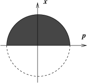
Figure 1: Profile describing $AdS_{5}\times RP^{5}$.

Figure 2: Profile describing $AdS_{5}\times S^{5}$, arising from D3 branes far from the orientifold.

The simplest example is the semi-circle centred at the origin, which seeds the geometry $AdS_{5}\times RP^{5}$. As a fluid profile, it is the ground state of $N$ free fermions in the semi-infinite harmonic oscillator. We may note right away that the quotienting destroys translational invariance in the $x-p$ plane and therefore the semi-circle has to be centred at the origin (Fig. 1). Here and in what follows, the fundamental part of the bubble is shaded while the $Z_{2}$ image is indicated with a dotted line to exhibit the fact that in the “upstairs” space this is a $Z_{2}$ invariant configuration.

We can also have circular configurations such as the one in Fig.2, where no part of the circle touches the horizontal axis. This arises as the near-horizon geometry of D3-branes parallel to, but far away from, an orientifold plane. This example shows that geometries which occur in the un-orientifolded case can also occur in the presence of the orientifold. All that is required is for the boundaries to be completely contained in the upper half-plane. The lack of translational invariance, alluded to above, means that the distance of the disc in this figure from the horizontal axis is physically meaningful, in contrast to the un-orientifolded case.

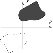
Figure 3: Bubble excluding the origin.

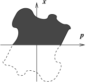
Figure 4: Bubble including the origin.

More general configurations are the union of bubbles of two basic types: those where the origin is included in the black region, and those where it is not. Examples of the two types are shown in Figs.3,4. From Fig.4 we notice that a boundary component of the latter type will be smooth only if, at the two points where it touches the real axis, the slope is the same.

As noted earlier, when the origin is in a black region there is an $RP^{3}$ in the spacetime geometry. This is the case for the bubble in Fig.4. For bubbles that do not include the origin, at first sight there appear to be two types: one illustrated in Fig.3 where the bubbles are completely contained in the upper half plane (along with their images in the lower half plane), and another type as in Fig.5 where the boundaries cross the horizontal axis at $x=0$.

Figure 5: Profile similar to Fig.3 after rotation.

The difference between these two examples is only superficial and can be eliminated by making a different choice of fundamental region. Choosing the right half plane as the fundamental region in Fig.5 puts the bubble completely inside the region, with its image on the other side. Thus we see that there are only two types of bubbles. Deforming these two types into each other leads to topology change via singular geometries, as we will see below.

In the models of Ref.[1], particular types of bubbles were identified with “giant gravitons”. These are bubbles consisting of a black region with a small hole inside, the area of the hole being much smaller than the area of the black region surrounding it. The corresponding geometries were interpreted as containing giant gravitons made up of D3-branes wrapping a maximal ${\tilde{S}}^{3}$ in $S^{5}$. In the orientifolded case we may instead consider a hole inside the bubble of Fig.1. We see that there are two types of such holes, and correspondingly two types of giant gravitons (Fig.6). If the small hole is in a generic location then we have giant gravitons wrapping a 3-sphere ${\tilde{S}}^{3}$ in $RP^{5}$. On the other hand if the hole surrounds the origin, we have giant gravitons wrapping an $RP^{3}$ cycle of $RP^{5}$.

Figure 6: Two types of giant gravitons in $AdS_{5}\times RP^{5}$.

Interestingly, as the hole around the origin becomes large enough to interpret this as a new back-reacted geometry, we find that the $RP^{3}$ cycle has disappeared – for the reason, stated earlier, that the black region does not enclose the origin. Also, when the hole expands further so that the black region forms a thin semicircular ring (stuck to the horizontal axis), we can interpret the configuration as consisting of dual giant gravitons wrapping an $S^{3}$ of $AdS_{5}$, and uniformly distributed around an equator of $RP^{5}$.

5.2 Torsion Cycles

A unique feature of the $AdS_{5}\times RP^{5}$ theory as compared to the unorientifolded case is the appearance of discrete torsion, as explained by Witten[17] and discussed in section 3. This means that there are topologically distinct configurations of the $B$-field, described by the theta angles $\theta_{NS\,NS}$ and $\theta_{RR}$. In this section, we wish to understand how this feature manifests itself in terms of the free fermion description on the distinguished $(x_{1},x_{2})$ geometry-seeding plane.

Figure 7: The path $T$, with endpoints $P$ and $Q$, intersects the $D3$ brane.

As a warm-up, consider first a $D3$ brane in $AdS_{5}\times S^{5}$. We may take it to be localized in the radial direction $\rho$ on $AdS_{5}$, as well as located at a point on the $S^{5}$. It then extends along an $S^{3}$ in the $AdS_{5}$. Suppose now that we choose a path $T$ whose endpoints are two points $P$ and $Q$ on opposite sides of the 3-brane, as shown in Fig.7. Consider the integral of $dF_{5}$ over the domain $T\times S^{5}$. Since the brane provides a source for the five-form flux $F_{5}$, and upon using Stokes’s theorem, we find

$$2\pi=\int_{T\times S^{5}}dF_{5}=\int_{P\times S^{5}}F_{5}-\int_{Q\times S^{5}}F_{5}.$$ (21)

We can conclude that the flux through the $S^{5}$ changes by one upon crossing the brane, changing the the gauge group from $SU(N)$ to $SU(N\pm 1)$. On the orientifold, the gauge group instead changes from $SO(2N)$, $SO(2N+1)$ or $Sp(2N)$ to $SO(2N\pm 2)$, $SO(2N+1\pm 2)$ or $Sp(2N\pm 2)$ respectively, since $RP^{5}$ is covered twice by $S^{5}$.

¿From the outset, the orientifolded theory has no preferred set of discrete torsion, i.e. theta angles $(\theta_{NS\,NS},\theta_{RR})$. However, once a particular set of values has been assigned to some region, discrete torsions will automatically be induced on the entire space, depending on the distribution of magnetic sources. In the absence of magnetic sources for the $B$-fields, the torsions are constant over the entire space.

However, $D5$ or $NS5$ branes wrapped on $RP^{2}$ cycles, forming effective $D3$ branes on $AdS_{5}$, do provide such sources. Crossing such a $D3$ brane will, in addition to changing the rank of the gauge group as we just described, also cause the discrete torsion to change.

More concretely, suppose we are wrapping a $D5$ brane on an $RP^{2}$ cycle. This will result in an effective $D3$ brane which additionally has an RR-form flux $H_{RR}=dB_{RR}$, which we choose to vanish to preserve supersymmetry. On the $AdS_{5}$ space, suppose the brane is again localized in the radial direction, but extended in the $S^{3}$ directions. On the $RP^{5}$, the brane is extended along an $RP^{2}$. This means that it must be localised on an $RP^{3}$, at least locally. The $RP^{2}$ and the $RP^{3}$ are generically intersecting at one point. Consider, then, the integral of $dH$ over $T\times RP^{3}$, where $T$ is the same path as before. Similar to the $dF_{5}$ integral dealt with previously, we now find

$$2\pi=\int_{T\times RP^{3}}dH=\int_{P\times RP^{3}}H-\int_{Q\times RP^{3}}H.$$ (22)

Hence, the theta angle $\theta_{RR}$ jumps upon crossing the brane.

Our objective is now to understand what this picture corresponds to on the LLM plane $(x_{1},x_{2})$ of [1]. An $AdS_{5}\times RP^{5}$ background geometry implies that we should start out with a “semicircular” black region centred at the origin. The quotation marks indicate that the correct designation of the geometry in the LLM plane requires taking the non-trivial identifications into account.

In general, an $RP^{i}$ submanifold is realized in $RP^{j}$, $i<j$, by the inclusion

$$(x_{1},\ldots,x_{i+1})\rightarrow(x_{1},\ldots,x_{i+1},0,\ldots,0).$$ (23)

To find an $RP^{2}$ inside $RP^{5}$, we must therefore choose three coordinates $\{\tilde{X_{1}},\tilde{X_{2}},\tilde{X_{3}}\}$ among the six embedding coordinates $\{X_{i}\}$, defined by Eq.(12). The remaining $X_{i}$’s should be set to zero.

For the $S^{3}$ of $AdS_{5}$ to separate two well-defined regions on the boundary plane, it should not shrink to zero size there. The magnetic $D3$ branes will then be associated with the white region. In this region, the radius of the $\tilde{S}^{3}$ embedded in $S^{5}$ shrinks to zero, corresponding to $\sin\theta=0$. Hence, $X_{1}=X_{2}=X_{3}=X_{4}=0$. We must therefore include at least one of the LLM coordinates in the generically non-vanishing set $\{\tilde{X}_{i}\}$, since otherwise the $X_{i}$’s cannot square to unity. Actually, $X_{5}$ and $X_{6}$ are only proportional to the LLM coordinates $x_{1}$ and $x_{2}$, differing by a $\rho$-dependent factor. Recalling Eq.(4), we can write

$$x_{1} =\sqrt{r_{0}}\,X_{5}\cosh\rho$$ (24)

$$x_{2} =\sqrt{r_{0}}\,X_{6}\cosh\rho.$$ (25)

This confirms that the brane will always be positioned outside of the black “semidisc” of radius $r_{0}\equiv R^{2}$.

Suppose first that precisely one of the two LLM coordinates belong to the generically non-vanishing set. All the other embedding coordinates must then vanish. Consequently, the non-vanishing coordinate, which is either $X_{5}$ or $X_{6}$, must be assigned the value $R$. Due to (25), this means that the brane appears as a point at radial position $r_{0}\cosh\rho$.

The other type of brane appears if we choose both of the LLM coordinates to belong to the generically non-vanishing set. Again, all other embedding coordinates vanish. The embedding condition then implies that $X_{5}^{2}+X_{6}^{2}=R^{2}=r_{0}$. Taking (25) into account, this leads us to conclude that in this case, the brane appears as a “semicircle” of radius $r_{0}\cosh\rho$. More precisely, the $RP^{2}$ collapses to an $RP^{1}$ in the LLM plane.

Figure 8: Magnetically charged $D3$ branes in an $AdS_{5}\times RP^{5}$ background.

In conclusion, we have found two different types of magnetic $D3$ branes, appearing on the LLM plane as illustrated in Fig.8. One type appears as points, restricted to lie on one of the axes. The positions of two such branes are indicated by black dots in the figure. The other type appears as $RP^{1}$ cycles, one of which is shown. Every such cycle divides the LLM plane into two parts, allowing these D-branes to separate regions of unequal discrete torsion $(\theta_{NS\,NS},\theta_{RR})$. In both cases, the $RP^{2}$ is completely collapsed onto the LLM plane. In addition, the branes extend along the $S^{3}$ directions of the $AdS_{5}$.

We have illustrated the ideas involved assuming an $AdS_{5}\times RP^{5}$ background, but our conclusions should be equally valid also for the other ${\frac{1}{2}}$-BPS geometries. In particular, the topology on the LLM plane, including the distribution of domain walls, is expected to reflect the topology of the full bulk geometry.

5.3 Topology Change

In the absence of orientifolds, topology change in the family of ${\frac{1}{2}}$-BPS geometries of LLM type takes place at a fermi fluid boundary satisfying a local equation[11] like $x_{1}\,x_{2}=0$. This can be thought of as a limit of the smooth boundary $x_{1}\,x_{2}=\mu$. Suppose this bounds a fermi fluid profile where for $\mu>0$ there is a single black region extending to infinity in, say, the upper left and lower right quadrants. Then for $\mu<0$ we have instead two separated black regions, one extending to infinity on the upper left and the other on the lower right. Clearly the connected black region splits into two disconnected ones as we pass through $\mu=0$ in the parameter space. It has been argued in Ref.[11] that this is the “irreducible” transition responsible for topology change, and that more general topology changes can be decomposed into a sequence of such transitions. The 10-dimensional geometry changes by the appearance or disappearance of $S^{5}$ factors.

Figure 9: Configuration of the topology of $AdS_{5}\times RP^{5}$, developing a neck.

Figure 10: Configuration of the topology of $AdS_{5}\times S^{5}$.

In the orientifolded theory there is another basic process of topology change that creates or destroys cycles of order two. The basic process of this type is the conversion of $RP^{5}$ into $S^{5}$ and vice versa. What happens is that an $AdS_{5}\times RP^{5}$ configuration consisting of a semi-disc anchored on the $x_{1}$ axis can be deformed until it develops a narrow neck connecting it to its image, as shown in Fig.9. At some stage the neck pinches off (Fig.10), and the bubble is no longer anchored to the horizontal axis.

Figure 11: Basic configuration for order-2 topology change.

Therefore this process represents a transition between $RP^{5}$ and $S^{5}$. We see that the origin was contained inside the bubble in the initial configuration, but is no longer contained at the end of the process. As we saw earlier, the former type of configuration has an $RP^{3}$ in the geometry while the latter does not. Thus this type of topology change causes us to lose or gain cycles of order two. At the transition, the (singular) configuration looks like a filled quadrant along with its mirror image, as shown in Fig.11. We expect that there will be topology-changing processes of “order $n$” built out of this basic process, as in Ref.[11].

6 M-theory Orientifolds

M-theory contains orientifold 5-planes[20, 21], so one can try to apply the construction above to this case. These orientifolds have been investigated further in Refs.[22, 23]. In particular one can take $N$ M5-branes parallel to an orientifold 5-plane, and the near-horizon geometry is $AdS_{7}\times RP^{4}$[24]. Unlike the D3-O3 system in type IIB string theory, here the sphere factor becomes non-orientable after quotienting. This is because the space transverse to the original branes (and the orientifold plane) was $R^{5}$, whose orientation is reversed upon reflection.

What is the effect of orientifolding on the $x_{1}-x_{2}$ plane of the LLM geometry? We cannot be as explicit as in the type IIB case. There we had a precise map between this plane and the phase space of free fermions. The orientifold plane was realised on the phase space as a wall, blocking off the region of $x<0$ (or more precisely identifying the lower half plane with a rotated copy of the upper half plane). Therefore this was also the case in the $x_{1}-x_{2}$ plane and one could easily characterise functions $z$ which gave rise to the general orientifolded ${\frac{1}{2}}$-BPS geometry – as we did in the previous sections.

In the M-theory case, the free fermions are related to ${\frac{1}{2}}$-BPS excitations of the $(2,0)$ theory on M5-branes and arise from the transverse coordinates of the brane which are realised as scalar fields of the $(2,0)$ theory. Since all the transverse directions are being orientifolded, we again expect the fermions to move in a semi-infinite harmonic oscillator. Though we have seen in section 2 that the map from the fermion phase space to the $x_{1}-x_{2}$ plane is not a simple identification, it was noted there that the topology of the two should be the same. Therefore we expect that the orientifold plane in the M-theory case is realised as the $x_{1}$ axis in the $x_{1}-x_{2}$ plane of the geometry just as for type IIB strings. In that case most of the considerations in this paper will go through and we can generate a precise collection of ${\frac{1}{2}}$-BPS bubbling orientifolds in M-theory. We leave a more detailed analysis of this system for future work.

7 Conclusions

We have found an infinite class of new ${\frac{1}{2}}$-BPS geometries in type IIB string theory and, somewhat less explicitly, in M-theory. These have the same local geometry as the so-called “bubbling geometries” of Ref.[1], but have global identifications. The geometries themselves have no orientifold plane and therefore the underlying string theory has no open-string sector, but the identifications can nevertheless be thought of as due to orientifold planes. The geometries have cycles of order 2, some of which support discrete torsion, in addition to the usual homology cycles. These backgrounds have the same amount of supersymmetry and, upto discrete factors, the same $SO(4)\times SO(4)$ symmetry as the original bubbling geometries. We saw that they are associated to free fermions in a half-oscillator potential, which in turn arise as the eigenvalues of matrices in the Lie algebra of $SO(2N),Sp(2N)$ and $SO(2N+1)$.

It would be interesting to extend these results to the $\frac{1}{4}$-BPS geometries associated to $D3-D7-O3-O7$ systems. The introduction of $D7$-branes leads to a varying axion-dilaton background and the associated bubbling geometries are fairly simple and have already been found in Ref.[26]. The introduction of orientifold 7-planes makes the system more interesting as it can then be related to “F-theory” compactifications[27, 28, 29]. It has been argued[30] that orientifold 7-planes are dynamical and behave in some regions of moduli space like non-perturbative D-branes (which at strong coupling exhibit remarkable effects including, for example, exceptional global symmetries[31, 32]). In this context, aspects of the AdS/CFT correspondence have been discussed in Refs.[33, 34] and it should be possible to find more general solutions of this kind using the bubbling prescription.

Finally, as we mentioned at the beginning, orientifolded bubbling geometries could be realised as local geometries of supersymmetric flux compactifications. Whenever the fermi fluid is localised in a bounded domain, the geometry is asymptotically $AdS_{5}\times RP^{5}$ (or $AdS_{5}\times S^{5}$), and therefore can be matched on to flat spacetime. But there might be a prescription as powerful as bubbling (with its connection to free fermions) that describes genuine compact geometries with orientifolds. This might make it much easier to classify supersymmetric flux vacua.

Appendix A Free fermions from matrix quantum mechanics

In this appendix, we show that free fermions emerge from all the traditional gauge groups. While some of this material is known or implicit in the matrix model literature, it is useful to compile all the needed results here.

The key observation is that

$$H = \sum_{i=1}^{m}{1\over\sqrt{g}}{\partial\over\partial\lambda_{i}}\sqrt{g}{\partial\over\partial\lambda_{i}}=\sum_{i=1}^{m}{1\over\Delta^{2}}{\partial\over\partial\lambda_{i}}\Delta^{2}{\partial\over\partial\lambda_{i}}$$ (26)

$$= {1\over\Delta}\,\sum_{i=1}^{m}{\partial^{2}\over\partial\lambda_{i}^{2}}\Delta,$$ (27)

where the measure factor $\sqrt{g}=\Delta^{2}$ is given by

$$(\Delta_{-})^{2}\hskip 56.9055pt SU(m)$$ (28)

$$(\Delta_{-})^{2}(\Delta_{+})^{2}(\Delta_{0})^{2}\hskip 56.9055pt Sp(N),N=2m$$ (29)

$$(\Delta_{-})^{2}(\Delta_{+})^{2}\hskip 56.9055pt SO(N),N=2m$$ (30)

$$(\Delta_{-})^{2}(\Delta_{+})^{2}(\Delta_{0})^{2}\hskip 56.9055pt SO(N),N=2m+1,$$ (31)

where we have defined

$$\Delta_{-} \equiv\prod_{i<j}^{m} (\lambda_{i}-\lambda_{j})$$ (32)

$$\Delta_{+} \equiv\prod_{i<j}^{m} (\lambda_{i}+\lambda_{j})$$ (33)

$$\Delta_{0} \equiv\prod_{i}^{m} \lambda_{i},$$ (34)

expressed in terms of the eigenvalues $\{\lambda_{i}\}_{i=1,2,\cdots,m}$. The last equality in (26) follows from the identity

$$\sum_{i=1}^{m}{\partial^{2}\over\partial\lambda_{i}^{2}}\Delta=0.$$ (35)

The relation (26) means that a factor of $\Delta$ can be absorbed by the wave function, giving rise to a system of free fermions.

It remains to establish (28). Let us begin by considering the unitary group, consisting of matrices $U$ satisfying $UU^{\dagger}=\mathbb{I}$. The Lie algebra $su(2)$ consists of anti-hermitian matrices $A^{\dagger}=-A$. An infinitesimal variation $\delta U=U^{-1}dU$ of a unitary matrix $U$ is an element of the Lie algebra, $\delta U^{\dagger}=-\delta U$.

The hermitian matrix A can be diagonalized using unitary matrices,

$$U^{-1}AU=\Lambda=\mbox{diag}(\lambda_{1},\lambda_{2},\cdots,\lambda_{m})$$ (36)

The significance is that we are trading degrees of freedom in the anti-hermitian matrix for those of the eigenvalues themselves and of the diagonalizing unitary transformation. Differentiating equation (36) and solving for $dA$ gives

$$\mbox{Tr }(dAdA^{\dagger})=\mbox{Tr }\left(2\delta U\Lambda\left[\delta U,\Lambda\right]+\left(d\Lambda\right)^{2}\right),$$ (37)

which is manifestly invariant under unitary similarity transformations. Hence it defines a metric on the space of antihermitian matrices.

Denoting matrix elements of a matrix $M$ by $M_{ij}$, this becomes

$$\mbox{Tr }(dAdA^{\dagger})=2\sum_{i<j}^{m}\delta u_{ij}\delta u_{ij}^{*}(\lambda_{i}-\lambda_{j})^{2}+\sum_{i=1}^{m}d\lambda_{i}^{2},$$ (38)

We can read off the measure

$$\sqrt{g}=(\Delta_{-})^{2},$$ (39)

(up to some numerical constant) in accordance with (28).

Next, we turn our attention to the symplectic gauge group $\mbox{Sp}(2m)$, consisting of matrices $S$ satisfying $S^{T}JS=J$, where

$$J = \pmatrix{0&\mathbb{I}\cr-\mathbb{I}&0},$$ (40)

where $\mathbb{I}$ is the $m\times m$ identity matrix. The Lie algebra sp(2m) then consists of matrices $A$ such that $A^{T}=JAJ$. Infinitesimal variations $\delta S=S^{-1}dS$ belong to the Lie algebra $\mbox{sp}(2m)$.

Again, a Lie algebra element can be diagonalized using symplectic matrices, $S^{-1}AS=\Lambda$. Differentiating $S^{-1}AS=\Lambda$ and solving for $dA$ gives

$$\mbox{Tr }(dAJdA^{T}J)=\mbox{Tr }\left(2\delta S\Lambda\left[\delta S,\Lambda\right]+\left(d\Lambda\right)^{2}\right).$$ (41)

Defining $(e_{PQ})_{LM}=\delta_{PL}\delta_{QM}$, a basis for $\mbox{sp}(2m)$ is

$$e_{j,k}^{1} \equiv e_{j,k}-e_{k+m,j+m}$$ (42)

$$e_{j,k}^{2} \equiv e_{j,k+m}+e_{k,j+m}$$ (43)

$$e_{j,k}^{3} \equiv e_{j,k}-e_{k+m,j+m}.$$ (44)

Note that since $0=\det(A-\lambda\mathbb{I})=-\det(A+\lambda\mathbb{I})$, eigenvalues come in pairs, $\{(\lambda_{i},-\lambda_{i})\}_{i=1,2,\cdots,m}$. Consequently, we can write $\Lambda$ on the form

$$\Lambda=\sum_{i=1}^{k}\Lambda_{i}e_{ii}^{1}=\mbox{diag}(\lambda_{1},\lambda_{2},\cdots,\lambda_{m},-\lambda_{1},-\lambda_{2},\cdots,-\lambda_{m}).$$ (45)

Similarly, we write $\delta S$ as

$$\delta S = \sum_{i=1}^{m}\delta S_{i}^{d}e_{ii}^{1}$$ (46)

$$+ \sum_{j<k}^{m}\left[\delta S_{jk}^{i}(e_{jk}^{1}+e_{kj}^{1})+\delta S_{jk}^{ii}(e_{jk}^{1}-e_{kj}^{1})\right]$$ (47)

$$+ \sum_{j\leq k}^{m}\left[\delta S_{jk}^{a}(e_{jk^{2}+e_{jk}^{3}})+\delta S_{jk}^{b}(e_{jk}^{2}-e_{jk}^{3})\right].$$ (48)

The reason for this particular expansion is that it will make the metric diagonal. Indeed, differentiating $S^{-1}AS=\Lambda$ and solving for $dA$ gives

$$\mbox{Tr }(dA^{T}JdAJ) =2 \sum_{i=1}^{m}d\lambda_{i}^{2}$$ (49)

$$+8 \sum_{j<k}(\lambda_{j}-\lambda_{k})^{2}\left[(\delta S_{jk}^{ii})^{2}-(\delta S_{jk}^{i})^{2}\right]$$ (50)

$$+8 \sum_{j\leq k}+(\lambda_{j}+\lambda_{k})^{2}\left[(\delta S_{jk}^{b})^{2}-(\delta S_{jk}^{a})^{2}\right].$$ (51)

Hence, the measure is

$$\sqrt{g}=(\Delta_{-})^{2}(\Delta_{+})^{2}(\Delta_{0})^{2},$$ (52)

as anticipated in (28).

The orthogonal gauge group remains to be analysed. Orthogonal matrices $O$ satisfy $OO^{T}=\mathbb{I}$, and corresponding Lie algebra elements are antisymmetric, $AA^{T}=-A$. The infinitesimal variation $\delta O=O^{-1}dO$ of an orthogonal matrix $O$ is antisymmetric, $\delta O^{T}=-\delta O$.

As in the symplectic case, the eigenvalues come in pairs, differing only by a sign. This means that $SO(2m)$ and $SO(2m+1)$ both have $m$ independent eigenvalues. Consider first the case $SO(2m)$. Using orthogonal similarity transformations, antisymmetric matrices can only be brought to the block-diagonal form

$$\Lambda = \pmatrix{\lambda_{1}\pmatrix{0&1\cr-1&0}&0&\cdots&0\cr 0&\lambda_{2}\pmatrix{0&1\cr-1&0}&\cdots&0\cr\cdots&\cdots&\phantom{\pmatrix{0&1\cr-1&0}}&\cdots\cr 0&0&\cdots&\lambda_{N}\pmatrix{0&1\cr-1&0}}$$ (53)

$$= i\sigma_{2}\otimes{\rm diag}(\lambda_{1},\lambda_{2},\ldots,\lambda_{N}).$$ (54)

Suppose that $O$ is the orthogonal matrix which block-diagonalizes the antisymmetric matrix $A$, i.e.

$$O^{-1}AO=\Lambda.$$ (55)

Differentiating equation (55) and solving for $dA$ gives

$$\mbox{Tr }(dAdA^{T})=-\mbox{Tr }\left(2\delta O\Lambda\left[\delta O,\Lambda\right]+\left(d\Lambda\right)^{2}\right).$$ (56)

Defining

$$\sigma^{0} \equiv\mathbb{I}_{2\times 2}=\pmatrix{+1&0\cr 0&+1}\hskip 42.67912pt\sigma^{2} \equiv i\sigma_{2}=\pmatrix{0&+1\cr-1&0}$$ (57)

$$\sigma^{1} \equiv\sigma_{1}=\pmatrix{0&+1\cr+1&0}\hskip 51.21504pt\sigma^{3} \equiv\sigma_{3}=\pmatrix{+1&0\cr 0&-1}$$ (58)

as a basis of real $2\times 2$ matrices in terms of the identity matrix $\mathbb{I}_{2\times 2}$ and the Pauli matrices $\{\sigma_{i}\}$, we can write the variation $\delta O$ as

$$\delta O = \pmatrix{\delta O_{11}\pmatrix{0&1\cr-1&0}&\delta O_{12}^{A}\sigma^{A}&\cdots&\delta O_{1N}^{A}\sigma^{A}\cdots\cr-\delta O_{12}^{A}\sigma^{A}&\delta O_{22}\pmatrix{0&1\cr-1&0}&\cdots&\delta O_{2N}^{A}\sigma^{A}\cr\cdots&\cdots&\phantom{\pmatrix{0&1\cr-1&0}}&\cdots\cr-\delta O_{1N}^{A}\sigma^{A}&-\delta O_{2N}^{A}\sigma^{A}&\cdots&\delta O_{NN}\pmatrix{0&1\cr-1&0}}$$ (59)

$$= \sigma^{A}\otimes\delta O^{A}+i\sigma_{2}\otimes{\rm diag}(\delta O_{11},\delta O_{22},\ldots,\delta O_{NN}).$$ (60)

The antisymmetric matrix $\delta O^{A}$ is defined such that the entry at row $i$ and column $j$ is the coefficient $\delta O_{ij}^{A}$. We are using the convention that repeated indices $A$ are summed over.

Using the forms (53) and (59), the metric (56) becomes

$$\mbox{Tr }(dAdA^{T})= - 4\sum_{i<j}\sum_{A=1,3}\left(\delta O_{ij}^{A}\right)^{2}(\lambda_{i}+\lambda_{j})^{2}$$ (61)

$$+ 4\sum_{i<j}\sum_{A=0,2}(-1)^{A/2+1}\left(\delta O_{ij}^{A}\right)^{2}(\lambda_{i}-\lambda_{j})^{2}+\sum_{i=1}^{m}d\lambda_{i}^{2}$$ (62)

Consequently, the measure is

$$\sqrt{g}=(\Delta_{-})^{2}(\Delta_{+})^{2},$$ (63)

as written in (28).

Consider now the gauge group $SO(2m+1)$. The analysis goes through in much the same way as for the $SO(2m)$ case, replacing

$$\delta O\rightarrow\delta O+\sum_{i=1}^{m}\sum_{B=0,1}\delta O_{i}^{B}\tau^{B}\otimes e_{i,2k+1},$$ (64)

where $\tau^{0}\equiv\pmatrix{1\cr 0}$, $\tau^{1}\equiv\pmatrix{0\cr 1}$. Similarly, $\Lambda$ is just extended with another row and column of zeros, since there are still only $m$ eigenvalues. With these modifications, the metric (61) gets an additional contribution,

$$\mbox{Tr }(dAdA^{T})\rightarrow\mbox{Tr }(dAdA^{T})+\sum_{i,B}\lambda_{i}^{2}(\delta O_{i}^{B})^{2}.$$ (65)

The measure (63) changes accordingly,

$$\sqrt{g}\rightarrow\sqrt{g}\prod_{i=1}^{m}\lambda_{i}^{2}=(\Delta_{-})^{2}(\Delta_{+})^{2}(\Delta_{0})^{2},$$ (66)

consistent with (28).

Note that the symplectic and orthogonal gauge groups share the following two features. The independent set of eigenvalues can always be chosen to be non-negative. In addition, absorbing a factor of $\Delta$ into the wave function makes the eigenvalues $\lambda_{i}$ repel not only each other, but also their images $-\lambda_{i}$. This is consistent with the orientifold interpretation, as explained in section 4.

References

- [1] H. Lin, O. Lunin and J. Maldacena, “Bubbling AdS space and 1/2 BPS geometries,” JHEP 0410 (2004) 025 [arXiv:hep-th/0409174].
- [2] S. Corley, A. Jevicki and S. Ramgoolam, “Exact correlators of giant gravitons from dual SYM theory,” Adv. Theor. Math. Phys. 5 (2002) 809 [arXiv:hep-th/0111222].
- [3] D. Berenstein, “A toy model for the AdS/CFT correspondence,” JHEP 0407 (2004) 018 [arXiv:hep-th/0403110].
- [4] M. M. Caldarelli and P. J. Silva, “Giant gravitons in AdS/CFT. I: Matrix model and back reaction,” JHEP 0408 (2004) 029 [arXiv:hep-th/0406096].
- [5] J. M. Maldacena, “The large limit of superconformal field theories and supergravity,” Adv. Theor. Math. Phys. 2 (1998) 231 [Int. J. Theor. Phys. 38 (1999) 1113] [arXiv:hep-th/9711200].
- [6] E. Witten, “Anti-de Sitter space and holography,” Adv. Theor. Math. Phys. 2 (1998) 253 [arXiv:hep-th/9802150].
- [7] S. S. Gubser, I. R. Klebanov and A. M. Polyakov, “Gauge theory correlators from non-critical string theory,” Phys. Lett. B 428 (1998) 105 [arXiv:hep-th/9802109].
- [8] J. A. Minahan and K. Zarembo, “The Bethe-ansatz for super Yang-Mills,” JHEP 03 (2003) 013 [arXiv:hep-th/0212208].
- [9] A. A. Tseytlin, “Spinning strings and AdS/CFT duality,” [arXiv:hep-th/0311139].
- [10] N. Beisert, “The dilatation operator of super Yang-Mills theory and integrability,” Phys. Rept. 405 (2005) 1-202 [arXiv:hep-th/0407277].
- [11] P. Horava and P. G. Shepard, “Topology changing transitions in bubbling geometries,” JHEP 0502 (2005) 063 [arXiv:hep-th/0502127].
- [12] G. Mandal, “Fermions from half-BPS supergravity,” [arXiv:hep-th/0502104].
- [13] L. Grant, L. Maoz, J. Marsano, K. Papadodimas and V. S. Rychkov, “Minisuperspace quantization of ‘bubbling AdS’ and free fermion droplets,” [arXiv:hep-th/0505079].
- [14] A. Dhar, “Bosonization of non-relativstic fermions in 2-dimensions and collective field theory,” [arXiv:hep-th/0505084].
- [15] J. Polchinski, “String theory. Vols. 1,2,”
- [16] C. V. Johnson, “D-branes,”
- [17] E. Witten, “Baryons and branes in anti-deSitter space,” JHEP 9807 (1998) 006 [arXiv:hep-th/9805112].
- [18] H. Verlinde, “Holography and compactification,” Nucl. Phys. B 580 (2000) 264 [arXiv:hep-th/9906182].
- [19] A. Bilal, “2-D Gravity from matrix models: An introductory review, and particularities of antisymmetric matrix models”, in the Proceedings of the 14th Johns Hopkins Workshop on Current Problems in Particle Theory, Debrecen, Hungary, 1990, eds. G. Domokos, Z. Horvath, S. Kovesi-Domokos, World Scientific 1991.
- [20] K. Dasgupta and S. Mukhi, “Orbifolds of M-theory,” Nucl. Phys. B 465 (1996) 399 [arXiv:hep-th/9512196].
- [21] E. Witten, “Five-branes and M-theory on an orbifold,” Nucl. Phys. B 463, 383 (1996) [arXiv:hep-th/9512219].
- [22] K. Hori, “Consistency condition for fivebrane in M-theory on orbifold,” Nucl. Phys. B 539 (1999) 35 [arXiv:hep-th/9805141].
- [23] E. G. Gimon, “On the M-theory interpretation of orientifold planes,” [arXiv:hep-th/9806226].
- [24] C. h. Ahn, H. Kim and H. S. Yang, “ SCFT and M theory on ,” Phys. Rev. D 59 (1999) 106002 [arXiv:hep-th/9808182].
- [25] D. Bak, S. Siwach and H. U. Yee, “1/2 BPS geometries of M2 giant gravitons,” [arXiv:hep-th/0504098].
- [26] J. T. Liu, D. Vaman and W. Y. Wen, “Bubbling 1/4 BPS solutions in type IIB and supergravity reductions on ,” [arXiv:hep-th/0412043].
- [27] C. Vafa, “Evidence for F-Theory,” Nucl. Phys. B 469 (1996) 403 [arXiv:hep-th/9602022].
- [28] D. R. Morrison and C. Vafa, “Compactifications of F-Theory on Calabi–Yau Threefolds - I,” Nucl. Phys. B 473 (1996) 74 [arXiv:hep-th/9602114].
- [29] D. R. Morrison and C. Vafa, “Compactifications of F-Theory on Calabi–Yau Threefolds - II,” Nucl. Phys. B 476 (1996) 437 [arXiv:hep-th/9603161].
- [30] A. Sen, “F-theory and Orientifolds,” Nucl. Phys. B 475 (1996) 562 [arXiv:hep-th/9605150].
- [31] K. Dasgupta and S. Mukhi, “F-theory at constant coupling,” Phys. Lett. B 385, 125 (1996) [arXiv:hep-th/9606044].
- [32] M. R. Gaberdiel and B. Zwiebach, “Exceptional groups from open strings,” Nucl. Phys. B 518, 151 (1998) [arXiv:hep-th/9709013].
- [33] A. Fayyazuddin and M. Spalinski, “Large superconformal gauge theories and supergravity orientifolds,” Nucl. Phys. B 535, 219 (1998) [arXiv:hep-th/9805096].
- [34] O. Aharony, A. Fayyazuddin and J. M. Maldacena, “The large limit of field theories from three-branes in F-theory,” JHEP 9807, 013 (1998) [arXiv:hep-th/9806159].