Using the tachyon DBI action proposal for the effective theory of non-coincident D_p-brane-anti-D_p-brane system, we study the decay of this system in the tachyon channel. We assume that the branes separation is held fixed, i.e., no throat formation, and then find the bounce solution which describe the decay of the system from false to the true vacuum of the tachyon potential. We shall show that due to the non-standard form of the kinetic term in the effective action, the thin wall approximation for calculating the bubble nucleation rate gives a result which is independent of the branes separation. This unusual result might indicate that the true decay of this metastable system should be via a solution that represents a throat formation as well as the tachyon tunneling.

1 Introduction

It was shown by Coleman [1] that in a scalar field theory with potential $V(\phi)$ which has both false vacuum, $\phi_{f}$, and true vacuum, $\phi_{t}$ (see fig.1), and with standard kinetic term, i.e.,

$$S = -\int d^{p+1}x\left(\frac{1}{2}(\partial_{a}\phi)^{2}+V(\phi)\right)\,,$$ (1)

where $a$ is a world volume index, there is always a vacuum tunneling from the false vacuum to the true vacuum. The false vacuum decays via a quantum mechanical tunneling process that leads to the nucleation of bubbles of true vacuum. The semiclassical calculation of the bubble nucleation rate per unit volume, $\Gamma$, is given by [1]

$$\Gamma \sim e^{-B}\,,$$ (2)

where B is obtained from the action of the bounce solution to the Euclideanized field equations. The ”overshoot” argument of Coleman [1] guarantees the existence of the bounce solution. This argument is the following: Consider the equation of motion of the Euclideanized action for maximal symmetric solution and for $p>0$

$$\ddot{\phi}+\frac{p}{r}\dot{\phi}=V^{\prime}\,.$$ (3)

This equation is like the equation of motion of a particle in the potential $-V$ with the time dependent kinetic friction term $p\dot{\phi}/r$ (see fig.1). The bounce solution is a solution of the above equation that starts with the initial condition $\dot{\phi}(0)=0$ and $\phi(0)=\phi_{0}$, and approaches $\phi(\infty)=\phi_{f}$ with zero velocity. Around the maximum of $-V$ one can safely write $V^{\prime}(\phi)\sim\mu^{2}(\phi-\phi_{t})$, where $\mu^{2}=V^{\prime\prime}(\phi_{t})>0$, hence the above equation can be written in the linear form

$$\ddot{\phi}+\frac{p}{r}\dot{\phi} = \mu^{2}(\phi-\phi_{t})\,.$$ (4)

In terms of new variable $(\phi-\phi_{t})=r^{(1-p)/2}\psi$, this equation converts to Bessel equation

$$\ddot{\psi}+\frac{1}{r}\dot{\psi}-\left(\mu^{2}+\frac{(1-p)^{2}}{4r^{2}}\right)\psi = 0\,,$$ (5)

whose solution is Bessel function $\psi(r)=I_{(p-1)/2}(\mu r)$. Hence the solution of $\phi$ is

$$\phi(r)-\phi_{t} = \Gamma(\frac{p+1}{2})(\phi(0)-\phi_{t})I_{(p-1)/2}(\mu r)\left(\frac{2}{\mu r}\right)^{(p-1)/2}\,\,.$$ (6)

If initially $\phi$ is very close to $\phi_{t}$, it will stay there for long time. After that time it rolls with negligible friction term and with finite velocity down the potential $-V$ toward the vacuum $\phi_{f}$ which is at lower energy. Hence, there is always an ”overshoot” point for any potential with both false and true vacuum. An approximated bounce solution (the thin-wall approximation) can be found for any potential [1]. In this approximation, the particle stays at true vacuum for a fixed period of time. Then it moves quickly without friction through the valley of the potential $-V$, and slowly comes to rest at false vacuum at time infinity. The form of this solution depends on details of the potential $V$.

Figure 1: A potential $V(\phi)$ which has two non-degenerate vacuum $\phi_{f}$ and $\phi_{t}$ with $V(\phi_{t})<V(\phi_{f})$, and potential $-V(\phi)$ which appears in the equation of motion of the Euclideanized action.

A physical system in string theory that should be described effectively by a field theory that has potential with both false and true vacuums, is the non-coincident D-brane-anti-D-brane system [2]. Apart from the complex tachyon which is a scalar field that has a potential with both false and true vacuums, the world-volume of this metastable system has massless transverse scalar fields as well. It has been pointed out in [21] that the true decay channel for this system is the following: the branes attract each other by long range gravitational forces, and then they annihilate each other via a direct appearance of tachyon instability. However, when branes separation is much larger than the string length scale, this system may decay in another way: through the tunnel effect by creation of a throat between the branes [21]. Assuming that the tachyon is frozen at the false vacuum, the authors have found a throat solution to the Euclideanized equation of motion of the massless scalar fields. The decay rate for nucleating this throat between the two branes was found to be given by

$$B_{scalar} = T_{p}\Delta^{p+1}\frac{\sqrt{\pi}}{\Gamma\left(\frac{p+3}{2}\right)}\left(\frac{p\Gamma(1-1/2p)}{\Gamma(1/2-1/2p)}\right)^{p}\,,$$ (7)

where $\Delta$ is the branes separation. This result truly indicates that as the branes separation goes to infinity the decay rate (2) goes to zero. It has been noted in [21] that if the branes are free to move in the space, the time scale of the gravitational approach for the decay is much smaller than that of the decay via the throat formation. However, there are situations where the latter time scale is dominate [6].

Having a scalar field in the effective action of $D\bar{D}$ which has both false and true vacuums, i.e., the tachyon field, it is natural to ask what happens to this system when tachyon tunnels from the false vacuum to the true vacuum. We are then interested in the bounce solution of the Euclieanized equation of motion of the tachyon field. In the first step, however, we assume that the branes are frozen at specific position in the transverse space, i.e., no throat formation, and consider only the tachyon as dynamical field. This bounce solution has been studied in [6] using two-derivative truncation of the BSFT effective action. In the present paper, however, we use the tachyon DBI action, proposed in [14, 5] for describing effectively the non-coincident brane-anti-brane system, to study this bounce solution. We shall find that in the thin-wall approximation, the decay rate for nucleating the bubble is given by

$$B_{tachyon} = T_{p}(\ell_{c})^{p+1}\frac{\sqrt{\pi}}{\Gamma\left(\frac{p+3}{2}\right)}(\sqrt{\pi}p/2)^{p}$$ (8)

where $\ell_{c}=\sqrt{2\pi^{2}\alpha^{\prime}}$. Unlike the result in (7), the above is independent of the branes separation! We interpret this unusual result as a sign that the assumption that there is no throat formation between the two branes is not a valid assumption. In other words, the true decay of the metastable $D\bar{D}$ system should be via a solution of the coupled equation of motion of massless scalar and tachyon which represents both tachyon bounce and scalar throat formation.

In the next section, we review the construction of the tachyon DBI action proposed in [14, 5] for the effective theory of non-coincident $D_{p}\bar{D}_{p}$ system. In section 3, using the assumption that the branes separation is constant, we study the bounce solution of the tachyon equation and calculate the bubble nucleation rate for large brane separation.

A tachyon DBI field theory has also been used to study the vacuum tunneling from false to the true vacuum [3]. The physical process studied in [3] is nucleation of spherical D-branes in the presence of an external RR electric field [4]. Using the description of D-branes as solitons of the tachyon field on non-BPS D-branes, they calculated the rate of spherical D-branes nucleation as the tachyon tunneling from false to the true vacuum and find exact agreement with the result in [4].

2 Review of construction of $D_{p}\bar{D}_{p}$ effective action

In this section we review the construction of the effective action of fixed D_p-brane-anti-D_p-brane proposed in [5]. Consider the effective action of one fixed non-BPS D_p-brane in type IIA(IIB) theory in flat background[7, 8, 9, 10]:

$$S = -\int d^{p+1}xV(T)\sqrt{-\det(\eta_{ab}+\alpha^{\prime}\partial_{a}T\partial_{b}T)}\,\,,$$ (9)

where $V(T)=T_{p}(1-T^{2}/4+O(T^{4}))$ is the tachyon potential. A potential which is consistent with S-matrix element calculation up to $T^{4}$ term is $V(T)=T_{p}\,e^{-T^{2}/4}$ [11]. This potential appears also in the BSFT tachyon effective action [12].

The kink solution of tachyon should be the BPS D_p-1-brane of type IIA(IIB) [13]. The tension of the kink is given by $T_{p-1}=\sqrt{\alpha^{\prime}}\int_{-T_{0}}^{T_{0}}V(T)dT$ where $T_{0}$ is the value of the tachyon potential at its minimum. There are many different tachyon potentials which correctly reproduce the tension of the BPS brane [14, 15], i.e., $T_{p-1}=\pi\sqrt{2\alpha^{\prime}}T_{p}$. One example is the following potential [16, 17]:

$$V(T)=\frac{T_{p}}{\cosh(T/\sqrt{2})}\,\,.$$ (10)

This has minimum at $T\rightarrow\pm\infty$ and behaves as $V(T)\sim e^{-T/\sqrt{2}}$ at $T\rightarrow\infty$. This potential is also consistent with the fact that there is no open string state at the end of the tachyon condensation [18].

The effective action of $N$ non-BPS D-branes should be the non-abelian extension of the effective action of one non-BPS D-brane [8]. For two fixed non-BPS D-branes and for trivial background, the effective action is [8]

$$S = -\int d^{p+1}x{\rm Tr}\left(V(T)\sqrt{\det(Q)}\sqrt{-\det\left(\eta_{ab}+T_{ab}\right)}\right)\,,$$ (11)

where the matrix $T_{ab}$ is

$$T_{ab} = \alpha^{\prime}\partial_{a}T\partial_{b}T+\frac{1}{2\pi}\partial_{a}T[X^{i},T](Q^{-1})_{ij}[X^{j},T]\partial_{b}T\,,$$

and matrix $Q^{i}{}_{j}$ is

$$Q^{i}{}_{j} = I\delta^{i}{}_{j}-\frac{i}{2\pi\alpha^{\prime}}[X^{i},X^{k}]\eta_{kj}-\frac{1}{(2\pi)^{2}\alpha^{\prime}}[X^{i},T][X^{k},T]\eta_{kj}\,.$$ (12)

The trace in the action (11) should be completely symmetric between all non-abelian expressions of the form $[X^{i},X^{j}],\partial_{a}T,[X^{i},T]$, and individual $T$ of the tachyon potential. The matrices $X^{i}$ and $T$ are

$$X^{i}=\pmatrix{X^{(11)i}&X^{(12)i}\cr X^{(21)i}&X^{(22)i}},\,\,T=\pmatrix{T^{(11)}&T^{(12)}\cr T^{(21)}&T^{(22)}}\,,$$ (13)

where superscripts $(11),(12),(21),(22)$ refer to the ends of open strings, e.g., $(12)$ means the open string with one end on brane $1$ and the other end on brane $2$.

Now, type IIA(IIB) converts to type IIB(IIA) under orbifolding by $(-1)^{F_{L}^{S}}$. In particular, a non-BPS $D_{p}$-brane of IIA(IIB) converts to BPS $D_{p}$-brane or anti-$D_{p}$-brane of IIB(IIA) theory [19]. Hence, two non-BPS $D_{p}$-branes of IIA(IIB) may convert to $D_{p}$-brane-anti-$D_{p}$-brane of IIB(IIA). This orbifolding converts the matrices (13) to the following:

$$X^{i}=\pmatrix{X^{(1)i}&0\cr 0&X^{(2)i}},\,\,T=\pmatrix{0&\tau\cr\tau^{*}&0}\,.$$ (14)

where we have changed the notation here, i.e., the superscripts $(1)$ and $(2)$ refer to the open string fields with both ends on brane $1$ and $2$, respectively, and $\tau(\tau^{*})$ refers to the tachyon with one end on brane $1(2)$ and the other end on brane $2(1)$. The above matrices satisfy the following relations:

$$[X^{i},X^{j}]=0,\,\,\, [X^{i},T]=\ell^{i}\pmatrix{0&\tau\cr-\tau^{*}&0},\,\,\,$$

where $\ell^{i}=X^{(1)i}-X^{(2)i}$ is the field that represents the distance between the two branes. We have assumed, however, that this field is constant. The matrix $Q^{i}{}_{j}$ simplifies to

$$Q^{i}{}_{j} = I\left(\delta^{i}{}_{j}+\frac{|\tau|^{2}}{(2\pi)^{2}\alpha^{\prime}}\ell^{i}\ell_{j}\right)\,.$$

The inverse of this matrix is

$$(Q^{-1})^{i}{}_{j} = I\left(\delta^{i}{}_{j}-\frac{|\tau|^{2}}{(2\pi)^{2}\alpha^{\prime}\det(Q)}\ell^{i}\ell_{j}\right)\,,$$ (15)

where

$$\det(Q) = I\left(1+\frac{|\tau|^{2}\ell^{2}}{(2\pi)^{2}\alpha^{\prime}}\right)\,.$$ (16)

The matrix $T_{ab}$ simplifies to

$$T_{ab} = \frac{\alpha^{\prime}}{\det(Q)}\left(\partial_{a}T\partial_{b}T\right)\,=\,\frac{\alpha^{\prime}}{\det(Q)}\pmatrix{\partial_{a}\tau\partial_{b}\tau^{*}&0\cr 0&\partial_{a}\tau^{*}\partial_{b}\tau}\,\,.$$ (17)

Note that this matrix is not a real matrix, however, one expects to have a real action after implementing the trace prescription.

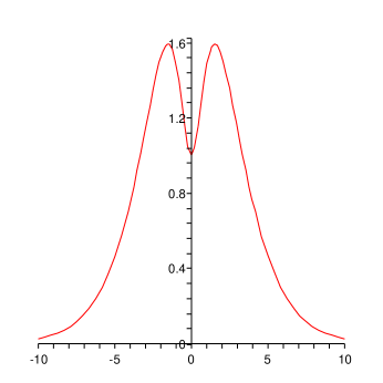
Figure 2: The $D_{p}\bar{D}_{p}$ potential ${\cal V}(\phi,\ell)$ for brane separation $\ell>\ell_{c}$ in terms of $\phi$.

Inserting the expressions (16) and (17) into (11), and performing the symmetric trace, one finds the following effective action for non-coincident $D_{p}\bar{D}_{p}$ system of IIB(IIA) theory:

$$S = -2\int d^{p+1}x\,{\cal V}(|\tau|,\ell)\left(\sqrt{-\det(\eta_{ab}+\frac{\alpha^{\prime}/2}{1+\frac{|\tau|^{2}\ell^{2}}{(2\pi)^{2}\alpha^{\prime}}}(\partial_{a}\tau\partial_{b}\tau^{*}+\partial_{a}\tau^{*}\partial_{b}\tau)}\right)\,,$$ (18)

where the tachyon potential is

$${\cal V}(|\tau|,\ell) = V(|\tau|)\sqrt{1+\frac{|\tau|^{2}\ell^{2}}{(2\pi)^{2}\alpha^{\prime}}}\,,$$ (19)

where $V(|\tau|)$ is the tachyon potential of the original non-BPS $D_{p}$-brane of IIA(IIB) theory, e.g., (10). Note that ${\cal V}(|\tau|,\ell=0)=V(|\tau|)$. See [20], for other proposal for the effective potential of non-coincident $D_{p}\bar{D}_{p}$ system. For $\ell>\ell_{c}$ where $\ell_{c}\equiv\sqrt{2\pi^{2}\alpha^{\prime}}$, the above potential has a barrier, see fig.2. Having two non-degenerate minima for the potential, one may expect that the $D_{p}\bar{D}_{p}$ system makes a bubble formation by tachyon tunneling through the barrier. In the next section we will study this tunneling.

3 Bounce solution of $D_{p}\bar{D}_{p}$ system

The tachyon potential depends only on the amplitude of the complex tachyon, hence , the phase of this field can be held fixed. Writing the complex tachyon as $\tau=\phi e^{i\theta}$, the action (18) for fixed $\theta$ becomes

$$S = -2\int d^{p+1}x{\cal V}(\phi,\ell)\sqrt{-\det\left(\eta_{ab}+\frac{\alpha^{\prime}}{1+\frac{\phi^{2}\ell^{2}}{(2\pi)^{2}\alpha^{\prime}}}\partial_{a}\phi\partial_{b}\phi\right)}\,\,\,,$$

This action can be rewritten as

$$S = -\frac{T_{p-1}}{\sqrt{\alpha^{\prime}}}\int d^{p+1}xU(\phi)\sqrt{1+\frac{\phi^{2}\ell^{2}}{(2\pi)^{2}\alpha^{\prime}}+\alpha^{\prime}\partial_{a}\phi\partial^{a}\phi}\,\,\,,$$

where we have rescaled the tachyon potential by $2\sqrt{\alpha^{\prime}}/T_{p-1}$ and $T_{p-1}$ is the tension of the BPS D_p-1-brane of type IIA(IIB), i.e., $U(\phi)=2\sqrt{\alpha^{\prime}}V(\phi)/T_{p-1}$. The tachyon potential is now dimensionless.

The Euclidean action is

$$S_{E} = \frac{T_{p-1}}{\sqrt{\alpha^{\prime}}}\int d^{p+1}xU(\phi)\sqrt{1+\frac{\phi^{2}\ell^{2}}{(2\pi)^{2}\alpha^{\prime}}+\alpha^{\prime}\partial_{a}\phi\partial^{a}\phi}\,\,\,.$$ (20)

The tachyon potential ${\cal V}$ has local minimum at $\phi=0$ and global minima at $\phi=\pm\infty$. Since the true vacuums are at infinity, it is convenient to define a new field as

$$\Phi = \int_{0}^{\phi}U(\phi^{\prime})d\phi^{\prime}\,\,.$$ (21)

In terms of this new field, the false vacuum is at $\Phi=0$ and the true vacuums are at $\Phi=\pm 1$. The value of the dimensionless tachyon potential, ${\cal Z}=2\sqrt{\alpha^{\prime}}{\cal V}/T_{p-1}$, at false vacuum is ${\cal Z}(0,\ell)=\sqrt{2}/\pi$, and at the true vacuums is ${\cal Z}(\pm 1,\ell)=0$.

For the potential (10), the relation between $\phi$ and $\Phi$ is $e^{\phi/\sqrt{2}}=\tan(\pi(1+\Phi)/4)$, and the tachyon potential ${\cal Z}$ is

$${\cal Z}(\Phi,\ell) = U(\Phi)\sqrt{1+\frac{\ell^{2}}{(2\pi)^{2}\alpha^{\prime}}\phi^{2}(\Phi)}$$

$$= \frac{\sqrt{2}}{\pi}\cos\left(\frac{\pi}{2}\Phi\right)\sqrt{1+\frac{\ell^{2}}{2\pi^{2}\alpha^{\prime}}\left[\ln\left(\tan\left(\frac{\pi}{4}(1+\Phi)\right)\right)\right]^{2}}\,\,.$$

In fig.3, $-{\cal Z}(\Phi,\ell)$ is plotted for different values of the brane separation $\ell$.

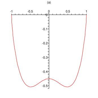
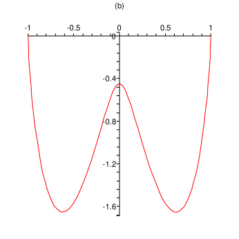
Figure 3: The potential $-{\cal Z}(\Phi,\ell)$ for a) $\ell^{2}=2\ell_{c}^{2}$ and for b) $\ell^{2}=30\ell_{c}^{2}$. The maximum and minimum of the potential is independent of $\ell$, however, the valley of the potential increases as $\ell$ increases.

We are interested in studying the tunneling from the local minimum $\Phi=0$ to the global minimum $\Phi=-1$ of the potential ${\cal Z}$. In terms of the new field (21), the action (20) becomes

$$S_{E} = \frac{T_{p-1}}{\sqrt{\alpha^{\prime}}}\int d^{p+1}x\sqrt{{\cal Z}^{2}(\Phi,\ell)+\alpha^{\prime}\partial_{a}\Phi\partial^{a}\Phi}\,\,\,.$$

Following [1], one has to find a solution with maximal symmetry, i.e., $\Phi=\Phi(r)$ where $r^{2}=x_{a}x^{a}$, and with the boundary conditions $\dot{\Phi}(0)=0$ and $\Phi(\infty)=\dot{\Phi}(\infty)=0$. For such a solution the above action becomes

$$S_{E} = \frac{T_{p-1}}{\sqrt{\alpha^{\prime}}}A_{p}I_{E}\,\,,$$ (23)

where $A_{p}$ is the area of the $p$-sphere with radius 1, i.e., $A_{p}=2\pi^{(p+1)/2}/\Gamma(1/2+p/2)$, and the effective one-dimensional action is

$$I_{E} = \int_{0}^{\infty}dr\,{\cal L}$$ (24)

$$= \int_{0}^{\infty}dr\,r^{p}\sqrt{{\cal Z}^{2}+\alpha^{\prime}\dot{\Phi}^{2}}\,\,.$$

The Euler Lagrange equation of motion is

$$\frac{\alpha^{\prime}\ddot{\Phi}Z^{2}}{(Z^{2}+\alpha^{\prime}\dot{\Phi}^{2})^{3/2}}+\frac{p}{r}\frac{\alpha^{\prime}\dot{\Phi}}{\sqrt{Z^{2}+\alpha^{\prime}\dot{\Phi}^{2}}} = \frac{ZZ^{\prime}}{\sqrt{Z^{2}+\alpha^{\prime}\dot{\Phi}^{2}}}(1+\frac{\alpha^{\prime}\dot{\Phi}^{2}}{Z^{2}+\alpha^{\prime}\dot{\Phi}^{2}})\,\,.$$ (25)

The second term on the left hand side represents friction term which decreases as time progresses. It is easier to work in the Hamiltonian formulation to study this nonlinear system. The equations of motion in the Hamiltonian formulation are

$$\dot{\Pi} = {\cal Z}^{\prime}\sqrt{1-\Pi^{2}/\alpha^{\prime}}-\frac{p}{r}\Pi\,\,,$$

$$\dot{\Phi} = \frac{{\cal Z}\Pi/\alpha^{\prime}}{\sqrt{1-\Pi^{2}/\alpha^{\prime}}}\,\,.$$ (26)

where $\Pi$ is related to the conjugate momentum of the field $\Phi$ as

$$\Pi = \frac{\alpha^{\prime}\dot{\Phi}}{\sqrt{{\cal Z}^{2}+\alpha^{\prime}\dot{\Phi}^{2}}}\,\,.$$ (27)

Note that $\Pi$ is bounded between $-\sqrt{\alpha^{\prime}}$ and $\sqrt{\alpha^{\prime}}$. The bounce solution is a solution of the above equations (26) with boundary conditions $\Pi(0)=0$ and $\Phi(\infty)=\Pi(\infty)=0$.

Because of the friction term for $p>0$, system is not conservative. It is still useful to consider the energy:

$$E\,\,\equiv\,\,\frac{1}{r^{p}}H = \frac{1}{r^{p}}\left(\dot{\Phi}\frac{\partial{\cal L}}{\partial\dot{\Phi}}-{\cal L}\right)$$ (28)

$$= -{\cal Z}\sqrt{1-\Pi^{2}/\alpha^{\prime}}\,\,.$$

Using (26), one can easily show that the lost of energy is

$$\dot{E} = -\frac{p}{\alpha^{\prime}r}\frac{{\cal Z}\Pi^{2}}{\sqrt{1-\Pi^{2}/\alpha^{\prime}}}\,\,=\,\,-F\dot{\Phi}\,\,,$$ (29)

where $F=p\Pi/r$ is the friction.

We now show that there is an ”overshoot” point for any brane separation. To see this, one has to study the behavior of the system near the true vacuum. Around the true vacuum, ${\cal Z}\sim 0$, the equations (26) are decoupled, i.e.,

$$\dot{\Pi} = {\cal Z}^{\prime}\sqrt{1-\Pi^{2}/\alpha^{\prime}}-\frac{p}{r}\Pi\,\,,$$

$$\dot{\Phi} \sim 0\,\,,$$ (30)

where ${\cal Z}^{\prime}$ is a very large number near the true vacuum.

We first consider $p=0$. In this case, the above equations have the following analytic solution:

$$\Pi(r)\,\,=\,\,\sqrt{\alpha^{\prime}}\sin({\cal Z}^{\prime}r/\sqrt{\alpha^{\prime}}) \Phi(r)\sim-1\,\,,\qquad\qquad{\rm for}\,\,r<\frac{\pi\sqrt{\alpha^{\prime}}}{2{\cal Z}^{\prime}}$$ ;

$$\Pi(r)\,\,=\,\,\sqrt{\alpha^{\prime}} \Phi(r)\sim-1\,\,,\qquad\qquad{\rm for}\,\,r\geq\frac{\pi\sqrt{\alpha^{\prime}}}{2{\cal Z}^{\prime}}\,\,.$$ ; (31)

At the time $R/\sqrt{\alpha^{\prime}}=\pi/(2{\cal Z}^{\prime})$, $\Pi$ reaches to its maximum value and stays there forever. In this case, conservation of energy guarantees the existence of the bounce solution, and the above result indicates that the initial value $\Phi(0)=\Phi_{0}$ of the bounce solution is larger than $-1$. One can find $\Phi_{0}$ by using the conservation of energy, i.e., ${\cal Z}(\Phi_{0})={\cal Z}(\Phi=0)$, or, in terms of old field,

$$U(\phi_{0})\sqrt{1+\frac{\ell^{2}}{(2\pi)^{2}\alpha^{\prime}}\phi_{0}^{2}} = U(0)\,\,.$$ (32)

The coefficient $B$ for the bounce solution is

$$B = \frac{T_{-1}}{\sqrt{\alpha^{\prime}}}\left(\int_{0}^{\infty}dr\sqrt{{\cal Z}^{2}+\alpha^{\prime}\dot{\Phi}^{2}}-\int_{0}^{\infty}drU(0)\right)$$ (33)

$$= T_{-1}\int_{\phi_{0}}^{0}\frac{\sqrt{U^{2}(\phi)\left(1+\frac{\ell^{2}}{(2\pi)^{2}\alpha^{\prime}}\phi^{2}\right)-U^{2}(0)}}{\sqrt{1+\frac{\ell^{2}}{(2\pi)^{2}\alpha^{\prime}}\phi^{2}}}d\phi\,\,,$$

where we have used conservation of energy to write $\dot{\Phi}$ in terms of energy and tachyon potential. Note that, for large $\ell$, the integral is independent of the brane separation, i.e., $B\sim T_{-1}\int_{-1}^{0}d\Phi=T_{-1}=\ell_{c}T_{0}$. We will show in the next section that this property is hold even for $p>0$ cases.

For $p>0$ cases, the qualitative form of the solution of equations (30) is the same as (31). However, because of the friction term $p\Pi/r$ in (30), $\Pi$ reaches to its maximum value in a bit longer than $R/\sqrt{\alpha^{\prime}}=\pi/(2{\cal Z}^{\prime})$. Then particle stays there for arbitrary long period of time by fine tuning the initial value of $\Phi$, i.e., the closer $\Phi$ to $-1$, the longer particle stays around $\Phi=-1$. After staying for arbitrary period of time at $\Phi\sim-1$, particle moves off this point with negligible friction toward the false vacuum. Therefore, there is an ”overshoot” point for any brane separation. In the next subsection we use the thin-wall approximation [1] to find the bounce solution for large brane separation.

3.1 The thin-wall approximation

We now find the bounce solution and calculate the coefficient B for large brane separation, and for $p>0$. The qualitative form of the bounce solution for large $\ell$ is the following: In order not to lose too much energy due to the friction, we must choose the initial position of the particle very close to $-1$. The particle then stays close to $-1$ until some very large time, $r=R$. Near time $R$, the particle moves quickly through the valley of the potential $-{\cal Z}$, and slowly comes to rest at $\Phi=0$ at time infinity, i.e.,

$$\Phi = -1\,,\qquad\qquad r<<R$$

$$= \Phi_{1}(r-R)\,,\,\,\,\,\,\,r\simeq R$$

$$= 0\,,\qquad\qquad\,\,\,\,\,\,r>>R$$

where $\Phi_{1}(r-R)$ is the solution that starts at $\Phi=-1$ with negligible friction term and ends at $\Phi=0$. Since the friction is neglected for this part, we can use conservation of energy to find this solution. Using the facts that energy is $E=-{\cal Z}\sqrt{1-\Pi^{2}/\alpha^{\prime}}$ and ${\cal Z}(-1)=0$, one observes that $\Pi=\sqrt{\alpha^{\prime}}$ during this period. From equation (27), one realizes that velocity of the particle should be infinite, i.e., $\dot{\Phi}_{1}=\delta(r-R)$. The only thing missing from this description is the value of $R$ which can be obtained by variational computation:

$$B = \frac{T_{p-1}}{\sqrt{\alpha^{\prime}}}A_{p}\left(\int_{0}^{\infty}drr^{p}\sqrt{{\cal Z}^{2}+\alpha^{\prime}\dot{\Phi}^{2}}-\int_{0}^{\infty}drr^{p}{\cal Z}(0)\right)$$

$$= \frac{T_{p-1}}{\sqrt{\alpha^{\prime}}}A_{p}\left(\int_{0}^{R}drr^{p}({\cal Z}(-1)-{\cal Z}(0))+\alpha^{\prime}R^{p}\int_{-1}^{0}\frac{d\Phi}{\Pi}\right)$$

$$= \frac{T_{p-1}}{\sqrt{\alpha^{\prime}}}A_{p}\left(-\frac{\epsilon}{p+1}R^{p+1}+\sqrt{\alpha^{\prime}}R^{p}\right)$$

where $\epsilon={\cal Z}(0)-{\cal Z}(-1)=\sqrt{2}/\pi$. Varying with respect to R, one obtains

$$\frac{dB}{dR}=0 \Longrightarrow R_{0}=\frac{p}{\epsilon}\sqrt{\alpha^{\prime}}\,=\,\frac{p}{2}\ell_{c}\,\,.$$ (36)

Thus the radius of the nucleated bubble is independent of the brane separation for large $\ell$. This is unlike the result in [6] that uses two-derivative truncation of the tachyon action. We note that the energy lost for the solution (3.1) is exactly equal to the difference energy between true and false vacuum, i.e.,

$$\Delta E = \int_{0}^{\infty}dr\,F\dot{\Phi}\,=\,\frac{p\sqrt{\alpha^{\prime}}}{R_{0}}\,=\,\epsilon$$ (37)

where we have replaced the radius of nucleated bubble from (36).

The condition for validity of the thin-wall approximation is [1]

$$\mu\left(\frac{R_{0}}{\sqrt{\alpha^{\prime}}}\right)>>1$$ (38)

where $\mu$ is the scale parameter of the theory. To find this parameter, we need to study the behaviour of the potential around its maximum, i.e.,

$${\cal Z}-{\cal Z}_{top} = \frac{1}{2}\mu(\delta\Phi)^{2}+\cdots$$ (39)

The dimensionless potential around the top of the hill is

$${\cal Z}-{\cal Z}_{top} \sim \frac{1}{2}\frac{\partial^{2}{\cal Z}}{\partial\phi^{2}}(\delta\phi)^{2}$$ (40)

$$= \frac{1}{2U^{2}}\frac{\partial^{2}{\cal Z}}{\partial\phi^{2}}(\delta\Phi)^{2}$$

For tachyon potential $U=(\sqrt{2}/\pi)e^{-\phi^{2}/4}$, and for large brane separation, i.e., $\ell>>\sqrt{\alpha^{\prime}}$, the maximum of the $D\bar{D}$ potential ${\cal Z}$ is at $\phi\sim\sqrt{2}$. For this case one finds

$$\mu = \frac{1}{U^{2}}\frac{\partial^{2}{\cal Z}}{\partial\phi^{2}}|_{\phi=\sqrt{2}}\,\sim\,\left(\frac{\sqrt{e}}{2}\right)\frac{\ell}{\sqrt{\alpha^{\prime}}}$$ (41)

For other tachyon potential, the numerical factor above changes. Therefore,

$$\mu\left(\frac{R_{0}}{\sqrt{\alpha^{\prime}}}\right) \sim \frac{p\pi}{2}\sqrt{\frac{e}{2}}\frac{\ell}{\sqrt{\alpha^{\prime}}}\,\,,$$ (42)

for large brane separation, the condition (38) is satisfied which means our thin-wall approximated solution (3.1) is valid. Note that, for the minimum value of the branes separation where there are false and true vacuums, i.e., $\ell=\ell_{c}$, the right hand side is $p\pi^{2}\sqrt{e}/2\sim 8p$ which is larger than one.

Finally, the decay width in the thin-wall approximation becomes

$$B = 2T_{p}A_{p}\left(-\frac{1}{p+1}R_{0}^{p+1}+\frac{1}{p}R_{0}^{p+1}\right)$$ (43)

$$= \frac{2T_{p}A_{p}}{p(p+1)}R_{0}^{p+1}$$

which is independent of brane separation $\ell$! Note that, the above result for $p=0$ gives $B=T_{0}\ell_{0}$ which is consistent with the result in (33) for large brane separation. This unusual result may indicate that the assumption that the transverse scalar fields of branes are fixed, i.e., no throat formation, is not a valid assumption. Or, it may indicates that the form of the effective action is not given by the tachyon DBI action when branes separation is larger than $\ell_{c}$.

To find the geometrical picture of the bubble, we note that in the approximated solution (3.1), inside the Euclidean sphere is filled with the true vacuum where the tachyon is completely condensed and so the brane-anti-brane are disappeared. Outside the sphere, on the other hand, is filled with the false vacuum where the tachyon does not condensed and so the brane-anti-brane do exist. The geometrical picture of brane-anti-brane after decay is then the original brane-anti-brane in which a spherical hole with radius (36) is created at the center of each brane, see fig.4. The radius of the bubble is independent of branes separation! These two holes may connect to each other by forming a throat [21, 6]. To study this throat formation, one has to release the assumption that the transverse scalars of the brane are fixed, and find a solution which includes both tachyon and the transverse scalar fields. In other words, one has to find a solution of the coupled equation of motion of massless scalar and tachyon which represents both tachyon bounce and the throat formation. One expects in this case that the radius of the hole depends on the branes separation, the larger the branes separation, the larger the radius of the hole. We leave this study for the future.

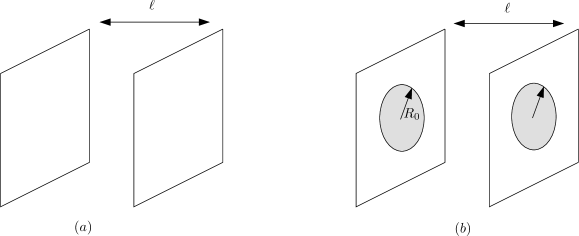
Figure 4: The time evolution of $D_{2}$-$\bar{D}_{2}$ system for condensation of tachyon into bounce solution. (a) Before decay. (b) After decay.

Acknowledgement: We would like to thank M.S. Costa, A. Ghodsi, K. Hashimoto, K. Javidan, G.R. Maktabdaran and J. Penedones for discussions. M.R.G would like to thank Perimeter Institute for hospitality.

References

- [1] S. Coleman, Phys. Rev D 15, 2929 (1977).
- [2] T. Banks and L. Susskind, “Brane-Anti-brane Force” arXiv:hep-th/9511194.
- [3] L. Cornalba, M. Costa, and J. Penedones, “Coleman meets Schwinger! ” arXiv:hep-th/0501151.
- [4] C. Teitelboim, Phys. Lett. B 167, 63 (1986).
- [5] M. R. Garousi, JHEP 0501, 029 (2005) [arXiv:hep-th/0411222].
- [6] K. Hashimoto, JHEP 0207, 035 (2002) [arXiv:hep-th/0204203].
- [7] A. Sen, HEP 9910, 008 (1999) [arXiv:hep-th/9909062].
- [8] M. R. Garousi, Nucl. Phys. B 584, 284 (2000) [arXiv:hep-th/0003122].
- [9] E. A. Bergshoeff, M. de Roo, T. C. de Wit, E. Eyras and S. Panda, JHEP 0005, 009 (2000) [arXiv:hep-th/0003221].
- [10] J. Kluson, Phys. Rev. D 62, 126003 (2000) [hep-th/0004106].
- [11] M.R. Garousi, JHEP 0305, 058 (2003) [arXiv:hep-th/0304145]; JHEP 0312, 036 (2003) [arXiv:hep-th/0307197].
- [12] P. Kraus and F. Larsen, Phys. Rev. D 63, 106004 (2001) [arXiv:hep-th/0012198]; T. Takayanagi, S. Terashima and T. Uesugi, JHEP 0103, 019 (2001) [arXiv:hep-th/0012210].
- [13] A. Sen, JHEP 9812, 021 (1998) [arXiv:hep-th/9812031]; P. Horava, Adv. Theor. Math. 2, 1373 (1999) [arXiv:hep-th/9812135].
- [14] A. Sen, Phys. Rev. D 68, 066008 (2003) [arXiv:hep-th/0303057].
- [15] M. Alishahiha, H. Ita and Y. Oz, Phys. Lett. B 503, 181 (2001) [arXiv:hep-th/0012222]; N.D. Lambert and I. Sachs, Phys. Rev. D 67, 026005 (2003) [arXiv:hep-th/0208217], Y. Kim, O.K. Kwon and C.O. Lee, arXiv:hep-th/0411164.
- [16] C.J. Kim, H.B. Kim, Y.B. Kim and O.K. Kwon, JHEP 0303, 008 (2003) [arXiv:hep-th/0301076]; F. Leblond and A.W. Peet, JHEP 0304, 048 (2003) [arXiv:hep-th/0303035].
- [17] N. Lambert, H. Liu and J. Maldacena, “Closed strings from decaying D-branes,” [hep-th/0303139].
- [18] A. Sen, “Field Theory of Tachyon Matter,” arXiv:hep-th/0204143.
- [19] A. Sen, “Non-BPS States and Branes in String Theory,” arXiv:hep-th/9904207.
- [20] I. Pesando, Mod. Phys. Lett. A 14, 1545 (1999) [arXiv:hep-th/9902181]; N. T. Jones and S.-H. Henry Tye, JHEP 0301, 012 (2003) [arXiv:hep-th/0211180].
- [21] C.G. Callen and J.M. Maldacena, Nucl. Phys. B 513, 198 (1998) [arXiv:hep-th/9708147].