Glueballs of Super Yang-Mills from wrapped branes

Elena Cáceres^† and Carlos Núñez^∗

^† CINVESTAV

Apdo. 14-740, 07000 Mexico D.F, Mexico.

and
Theory Group, Department of Physics, University of Texas at Austin

Austin, TX 78712, USA

^∗ Center for Theoretical Physics, Massachusetts Institute of Technology

Cambridge, MA 02139, USA

ABSTRACT: In this paper we study qualitative features of glueballs in ${\cal N}=1$ SYM for models of wrapped branes in IIA and IIB backgrounds. The scalar mode, $0^{++}$ is found to be a mixture of the dilaton and the internal part of the metric. We carry out the numerical study of the IIB background. The potential found exhibits a mass gap and produces a discrete spectrum without any cut-off. We propose a regularization procedure needed to make these states normalizable.

UTTG-05-05

MIT-CPT 3651

hep-th/0506051

1 Introduction and General Ideas

During the sixties the study of hadronic particles was a mainstream area of theoretical Physics. The Regge trajectories were proposed and by the systematic study of scattering of Hadrons, the dualities between the $s$ and $t$ channels amplitudes were investigated and nicely realized by the Veneziano amplitude,

The dual models, precursors of the modern String Theory, were one of the best candidates to explain the relevant Physics and provided the tools to explore the issues mentioned above. Despite some success, the experiments realized during the late sixties involving scatterings of large $s$ and large $t$ Mandelstam variables, but keeping fixed $\frac{s}{t}$ (fixed angle processes), gave results that showed that the amplitude was falling as a power law instead of the exponential law predicted by the dual models. This situation, together with the advent of QCD (that correctly predicted the scaling for fixed angle scattering and many other things), lead to the demise of the dual models for the study of hadronic Physics.

Even when the original motivation to study dual models momentarily dissapeared, their rich structure kept many physicists interested and, after some technical subtleties were understood, this was the beginning of String Theory.

As is known, after thirty years, string theorists have come back to the study of problems related to the hadronic world. Indeed, guided by the Maldacena Conjecture [1] and their refinements [2], there have been very many interesting achievements in the area. They correspond to field theories with different amount of SUSY (including no SUSY) but “very similar” to QCD. The important point is that many characteristic features of QCD, like confinement, chiral symmetry breaking, etc; have been understood based on dual String theory backgrounds.

In this paper, we study glueballs in some of the models mentioned above as being “very similar” to QCD (even when the models we will deal with here and those available in the literature, perhaps are not in the same universality class of QCD). Let us motivate a little bit the study of these glue-composed excitations.

We know that the main distinction between a field theory in a confining phase and the same field theory in the Higgs phase is the presence of Regge trajectories, that do not occur in theories with Coulomb of Yukawa interactions. These Regge trajectories appear when plotting the spin $J$ and the squarred mass $m^{2}$ of the excitation, thus giving relation of the form $J=\alpha^{\prime}m^{2}+\alpha_{0},$ with $\alpha^{\prime}\approx(1GeV)^{-2}$; this relation does not have in principle, an upper bound in $J,m$. It is due to these infinite number of Regge resonances, being interchanged in the $s,t$ channels of any hadron scattering that the beautiful structure of duality appeared in the models above mentioned. The glueballs should be some of these Regge excitations (making up a full trajectory if mixing with quarks is neglected) and this is a possible motivation to study them.

From a modern QCD perspective, it is known that the cloud of gluons is what logically connects between a current quark (with mass of a few $MeV$) to a constituent quark, with mass of around 300 $MeV$. Since glue is part of the hadronic matter, we can consider color singlet composites of the form $q\bar{q}g,\;gg,\;ggg$ (apart from the mesons, baryons and exotics). The glueballs are composites made out of constituent glue, with no quark content. Of course, since we live in a world with quarks, one might think that the proposal of pure glue objects is impossible to study, because the quarks should run in loops when doing corrections to the operators, that leads to glueballs mixing with mesons, rendering the object not-pure glue. But lattice theorist (working in the quenched approximation) are not stopped by this. Indeed they took advantage of the limitation and have taught us many things about glueballs.

Among the things that Lattice showed about QCD glueballs, we can mention the facts that:

• there is a bound state spectrum

• the lightest glueball is a scalar

• the next is a tensor, 1.6 times heavier

• the mass of the lightest glueball should be around 1630 $MeV$;

see for example [3] for a nice and clear review of these results.

How are these lattice predictions experimentally checked? Experimentalist look for processes rich in glue production, like the $J/\psi$ decay, where the $c,\bar{c}$ quarks annihilate into gluons. Other process might be the $p\bar{p}$ annihilation, in this case the idea is that the quarks and anti-quarks in the initial hadrons annihilate completely, producing glue that later decays into hadrons. There are many glueballs candidates. One of them seems to be well established and is called $f_{0}(1500)$ with a width of $112\;MeV$ [4].

From the string theory view point, using the Maldacena duality for the case of confining backgrounds, the study of glueballs (in the field theory dual to the background) proceeds by finding bound states for the fluctuations of the supergravity fields. Basically, the idea is to fluctuate all the fields in a given IIA, or IIB solution dual to a confining field theory, and linearizing in the fluctuated fields, study their eqs of motion (that are the Einstein, Maxwell and Bianchi eqs). The system is reduced to a Schroedinger problem. When solved, has eigenfunctions that we identify with the glueballs and eigenvalues that are identified with their masses. The fluctuations of the fields are dual to different operators in the gauge theory and what we are actually computing in the field theory side is the two-point correlation function of two glueball operators that should behave in a Wilson expansion as

$$<O(x)O(y)>=\sum_{j}c_{j}e^{M_{j}|x-y|}$$

where $M_{j}$ are the glueball masses. The quantum numbers of the glueballs $J^{PC}$ are determined on the basis of the spin ($J$) of the supergravity field and the R-symmetry quantum numbers (in a KK-harmonics decomposition) as studied, for example, in [5]. We should point that this procedure is not totally clear in many of the available confining-models and it should be important to understand it better.

This machinery has been applied to some confining models. Let us add that, since many of the existing Supergravity models are duals to confining field theories with only adjoint matter content, the objects under study are only glueballs (no hybrids) and since we work in the large $N_{c}$ regime, the glueballs are stable.

Let us briefly review what was done in this subject. the original idea, described above, has been proposed by Witten in [6]. Many papers followed, exploring this nice idea in different contexts. For example, confining models using black hole geometries were developed for $QCD_{3}$ and $QCD_{4}$ in [7], [8]. Also, models based on rotating branes were introduced [9] and other models based on $AdS_{5}$ with no SUSY [10]. All these models have an spectrum that is numerically very close to the one obtained by Lattice methods.

We should stress, that even when the comparisons between the lattice and “AdS” based results seem so accurate and promising, these calculations are done in opposite regimes. Indeed, the gravity-dual computation is in strong ’t Hooft coupling and this limitation is imposed by the Supergravity approximation. On the other hand, the Lattice computations are done at weak coupling, this seems to be a necessity of having a continuum limit because the lattice spacing $a$, has a relation $a\Lambda_{QCD}\approx e^{-1/g^{2}N}$ with the QCD coupling and scale (other regularizations give similar results). One might think about doing strong coupling lattice computations, but they do not seem to be smoothly related to the continuum theory. It is possible that the numerical coincidences aluded above, are based on some dynamical principle to be understood.

There exist a set of Supergravity models that preserve $N=1$ SUSY that have been object of lots of study and amusing advances. One of the models was put forward by Klebanov and Strassler [11] and the glueballs in this model were carefully studied in the set of papers [12],[13]. The results indicate that, for the Klebanov-Strassler model, the masses of the $0^{++},\;1^{--},\;2^{++}$ in the strong ’t Hooft coupling limit, fall in a linear trajectory. Also, the finding of a massless excitation showed that this cascading field theory is not in the same universality class of QCD, because of the reasons we explained above.

1.1 Motivations and organization of this paper

We mentioned above a set of Supergravity duals to confining models and up to this point we just commented on the one proposed by Klebanov and Strassler [11]. There exist some other models that are based on wrapped D-branes. The main idea here is to consider the low energy field theory in $(k+1)$ dimensions, obtained by wrapping a Dp brane on a $(p-k)$ cycle. Some subtleties of this type of models will be explained in section 2 of this paper. Here we just want to emphasize that the glueballs spectrum in this case is poorly understood.

Indeed, there is a paper [14], where a study was initiated. We believe that this study is not completely correct from a technical viewpoint (we believe that incorrect eqs were used) and the conclusions expressed there are, even when intuitively understandable, also not totally correct. The main point of that paper is that in one of these models it is necessary to introduce a hard cut-off in order to have a discrete spectrum. In this paper we re-analize this statement and propose a different result, basically that all these models do have discrete spectrum of glueballs and give a way of computing it. The spectrum even though discrete is not normalizable. In order to get normalizable states we need to introduce a regularization procedure. The regularization we propose is not the introduction of a hard cut-off but is more in the spirit of the Wilson loop calculations [16],[17] where a non-physical part is subtracted. In this paper we will not make much emphasis on the numerical aspects of the problem. Indeed, even when discrete states are numerically obtained, we will not worry here about comparisons with lattice results, that as explained above are perhaps not very significative. The main objective of this work is to study qualitative features of the spectrum, point out differences with previously studied cases, and propose a procedure of computing and regularizing in these wrapped branes set-ups.

This paper is divided in two parts, one dealing with a particular type IIB model and the other with a type IIA model. Both parts have been written and can be read in parallel and almost independently.

In section 2, we describe in detail the two models we will be using, one based in type IIB, with D5 branes wrapping a two-cycle inside the resolved conifold. The other in type IIA, based on D6 branes wrapping a three cycle in the deformed conifold. Section 3 deals with the glueballs in the type IIB set-up, while section 4 sketches the results corresponding to the type IIA model. We did not carry the problem to an end because of the need of a more precise numerical analysis, since the solution is only numerically known. Section 5 presents conclusions and possible future work proposed to the interested reader. There are very detailed Appendixes that carefully explain all the computations in sections 3 and 4.

2 ${\cal N}=1$ SYM models from wrapped branes

In this section, we write an account of duals to N=1 SYM from wrapped branes. The two main models on which we will concentrate are the ones based on D5 branes wrapping a two cycle, that we will consider to be a two-sphere inside a CY3 fold and D6 branes on a three cycle (a squashed three sphere), also inside a CY3 fold. We will present the solutions in detail, and explain the main characteristics of the dual gauge theory. We will emphasize the existence of ‘extra’ modes called KK modes with mass of the same order of the confinement scale. Since our interest in this paper is on glueballs, we will discuss the influence of this ‘extra’ modes in the computation of glueballs for $N=1$ SYM.

2.1 D5 branes wrapping $S^{2}$

We will work with the model presented in [18] (the solution was first found in a 4d context in [19]) and described and studied in more detail in the paper [20]. Let us briefly describe the main points of this supergravity dual to $N=1$ SYM and its UV completion.

Suppose that we start with N $D5$ branes, the field theory living on them is $(5+1)$SYM with 16 supercharges. Then, suppose that we wrap two directions of the D5 branes on a curved two manifold that can be choosen to be a sphere. In order to preserve SUSY a twisting procedure has to be implemented. The one we will be interested in this section, deals with a twisting that preserves four supercharges. In this case the two-cycle mentioned above lives inside a CY3 fold. Notice that this supergravity solution will be dual to a four dimensional field theory, only for low energies (small values of the radial coordinate). Indeed, at high energies, the modes of the gauge theory start to explore the two cycle and the theory becomes first N=1 SYM in six dimensions and then, the blowing-up of the dilaton forces us to S-dualize and a little string theory completes the model in the UV. In this sense, to study only the 4d-SYM part of the background, a procedure that “substracts” the unwanted UV completion, should be useful. We will elaborate on this in Section 3.1.

The supergravity solution corresponding to the case of interest in this section, the one preserving four supercharges, has the topology of $R^{1,3}\times R\times S^{2}\times S^{3}$ and there is a fibration between the two spheres that allows the SUSY preservation. The topology of the metric, near $r=0$ is $R^{1,6}\times S^{3}$. The full solution and Killing spinors are written in detail in [20]. Let us revise it here for reference. The metric in Einstein frame reads,

$$ds^{2}_{10}\,=\,\alpha^{\prime}g_{s}Ne^{{\phi\over 2}}\,\,\Big{[}\,\frac{1}{\alpha^{\prime}g_{s}N}dx^{2}_{1,3}\,+\,e^{2h}\,\big{(}\,d\theta^{2}+\sin^{2}\theta d\varphi^{2}\,\big{)}\,+\,dr^{2}\,+\,{1\over 4}\,(w^{i}-A^{i})^{2}\,\Big{]}\,\,,$$ (2.1)

where $\phi$ is the dilaton. The angles $\theta\in[0,\pi]$ and $\varphi\in[0,2\pi)$ parametrize a two-sphere. This sphere is fibered in the ten dimensional metric by the one-forms $A^{i}$ $(i=1,2,3)$. Their expression can be written in terms of a function $a(r)$ and the angles $(\theta,\varphi)$ as follows:

$$A^{1}\,=\,-a(r)d\theta\,,\,\,\,\,\,\,\,\,\,A^{2}\,=\,a(r)\sin\theta d\varphi\,,\,\,\,\,\,\,\,\,\,A^{3}\,=\,-\cos\theta d\varphi\,.$$ (2.2)

The $w^{i}\,$’s appearing in eq. (2.1) are the $su(2)$ left-invariant one-forms, satisfying

$$w^{1} = \cos\psi d\tilde{\theta}\,+\,\sin\psi\sin\tilde{\theta}d\tilde{\varphi}\,\,,$$

$$w^{2} = -\sin\psi d\tilde{\theta}\,+\,\cos\psi\sin\tilde{\theta}d\tilde{\varphi}\,\,,$$

$$w^{3} = d\psi\,+\,\cos\tilde{\theta}d\tilde{\varphi}\,\,.$$ (2.3)

The three angles $\tilde{\varphi}$, $\tilde{\theta}$ and $\psi$ take values in the rank $0\leq\tilde{\varphi}<2\pi$, $0\leq\tilde{\theta}\leq\pi$ and $0\leq\psi<4\pi$. For a metric ansatz such as the one written in (2.1) one obtains a supersymmetric solution when the functions $a(r)$, $h(r)$ and the dilaton $\phi$ are:

$$a(r) = {2r\over\sinh 2r}\,\,,$$

$$e^{2h} = r\coth 2r\,-\,{r^{2}\over\sinh^{2}2r}\,-\,{1\over 4}\,\,,$$

$$e^{-2\phi} = e^{-2\phi_{0}}{2e^{h}\over\sinh 2r}\,\,,$$ (2.4)

where $\phi_{0}$ is the value of the dilaton at $r=0$. Near the origin $r=0$ the function $e^{2h}$ behaves as $e^{2h}\sim r^{2}$ and the metric is non-singular. The solution of the type IIB supergravity includes a Ramond-Ramond three-form $F_{(3)}$ given by

$$\frac{\alpha^{\prime}}{N}F_{(3)}\,=\,-{1\over 4}\,\big{(}\,w^{1}-A^{1}\,\big{)}\wedge\big{(}\,w^{2}-A^{2}\,\big{)}\wedge\big{(}\,w^{3}-A^{3}\,\big{)}\,+\,{1\over 4}\,\,\sum_{a}\,F^{a}\wedge\big{(}\,w^{a}-A^{a}\,\big{)}\,\,,$$ (2.5)

where $F^{a}$ is the field strength of the su(2) gauge field $A^{a}$, defined as:

$$F^{a}\,=\,dA^{a}\,+\,{1\over 2}\epsilon_{abc}\,A^{b}\wedge A^{c}\,\,.$$ (2.6)

The different components of $F^{a}$ are:

$$F^{1}\,=\,-a^{\prime}\,dr\wedge d\theta\,\,,\,\,\,\,\,\,\,\,\,\,F^{2}\,=\,a^{\prime}\sin\theta dr\wedge d\varphi\,\,,\,\,\,\,\,\,\,\,\,\,F^{3}\,=\,(\,1-a^{2}\,)\,\sin\theta d\theta\wedge d\varphi\,\,,$$ (2.7)

where the prime denotes derivative with respect to $r$. Since $dF_{(3)}=0$, one can represent $F_{(3)}$ in terms of a two-form potential $C_{(2)}$ as $F_{(3)}\,=\,dC_{(2)}$. Actually, it is not difficult to verify that $C_{(2)}$ can be taken as:

$$\frac{\alpha^{\prime}C_{(2)}}{N} = {1\over 4}\,\Big{[}\,\psi\,(\,\sin\theta d\theta\wedge d\varphi\,-\,\sin\tilde{\theta}d\tilde{\theta}\wedge d\tilde{\varphi}\,)\,-\,\cos\theta\cos\tilde{\theta}d\varphi\wedge d\tilde{\varphi}\,-$$ (2.8)

$$-a\,(\,d\theta\wedge w^{1}\,-\,\sin\theta d\varphi\wedge w^{2}\,)\,\Big{]}\,\,.$$

Moreover, the equation of motion of $F_{(3)}$ in the Einstein frame is $d\Big{(}\,e^{\phi}\,{}^{*}F_{(3)}\,\Big{)}=0$, where $*$ denotes Hodge duality. Let us stress here that the previous configuration is non-singular.

Finally, let us comment on the fact that the BPS equations also admit a solution in which the function $a(r)$ vanishes, i.e. in which the one-form $A^{i}$ has only one non-vanishing component, namely $A^{3}$. We will refer to this solution as the “abelian” (or “singular”) ${\cal N}=1$ background. Its explicit form can be easily obtained by taking the $r\rightarrow\infty$ limit of the functions given in eq. (2.4). Notice that, indeed $a(r)\rightarrow 0$ as $r\rightarrow\infty$ in eq. (2.4). Neglecting exponentially suppressed terms, one gets:

$$e^{2h}\,=\,r\,-\,{1\over 4}\,\,,\,\,\,\,\,\,\,\,\,\,\,\,\,\,\,\,\,\,(a=0)\,\,,$$ (2.9)

while $\phi$ can be obtained from the last equation in (2.4). The metric of the abelian background is singular at $r=1/4$ (the position of the singularity can be moved to $r=0$ by a redefinition of the radial coordinate). This IR singularity of the abelian background is removed in the non-abelian metric by switching on the $A^{1},A^{2}$ components of the one-form (2.2).

2.2 Some analysis of this model

Let us first summarize the field theory aspects of the dual to the gravity solution we will be mainly concerned with. The main characteristic is that it contains a four dimensional Minkowski space, a radial direction and a two sphere fibered over a three sphere. In [18] this solution was argued to be dual to $N=1$ SYM. Let us analize the claim a little more, the field theory at low energies (low compared to the inverse size of the two-sphere) has degrees of freedom given by a vector field and a Majorana spinor (in 4d). When increasing in energy, other modes with mass of the order of the inverse size of the $S^{2}$ appear in the spectrum. These are called KK modes and can be seen as coming from the reduction of the maximally D5 branes SUSY field theory on a two dimensional sphere and a twisting (explained below) are performed. When the energy is high enough the excitations of the theory propagate in $5+1$ dimensions and the UV-completion of our minimally SUSY four dimensional field theory is the six dimensional little string theory living on $N$ NS5 branes.

Let us recall briefly the twisting procedure. One has a $5+1$ field theory (that lives on $N$ D5 branes) that has gauge fields, fermions and four scalars, all in the adjoint of the $SU(N)$ gauge group. We rewrite the $SO(1,5)\times SU(2)_{L}\times SU(2)_{R}$ group quantum numbers of the fields above in terms of $SO(1,3)\times SO(2)\times SU(2)_{L}\times SU(2)_{R}$ and then we mix the quantum numbers respect to $SO(2)$ with those of another $SO(2)$ that lives inside one of the $SU(2)^{\prime}s$. After this twisting procedure is performed, we are left with fields that under $SO(1,3)\times U(1)\times SU(2)$ transform as

$$A^{a}_{\mu}=(4,0,1),\;\;\Phi^{a}=(1,\pm,1),\;\;\phi^{a}=2(1,\pm,2).\;\;$$ (2.10)

for the bosons that can be seen to be a massless gauge field, a massive scalar (coming from the gauge field) and other massive scalars (that originally represented the positions of the D5 branes in $R^{4}$). As a general rule, all the fields that do transform under the twisted $U(1)$, the second entry in the charges above, will be massive. For the fermions we will have

$$\psi^{a}=(2,0,1),\;(\bar{2},0,1),\;\;(2,++,1),\;(\bar{2},--,1),\;(2,0,2),\;(\bar{2},0,2)$$ (2.11)

that is a Majorana spinor in four dimensions that is massless and then we have massive ones (those whose quantum number under the twisted $U(1)$ is not zero). The KK modes are the massive modes mentioned above. Their mass is of the order $M_{KK}^{2}=(R_{S2})^{-2}=\frac{1}{g_{s}\alpha^{\prime}N}$.

The dynamics of these KK modes, mixes with the dynamics of confinement in this model, because the scale of strong coupling of the theory is of the order of the KK mass. If we could work with a sigma model for the string in this background (or in the S-dual NS5 background) to all orders in $\alpha^{\prime}$ we could decouple both behaviours. Meanwhile, the dynamics of these KK modes has not been studied in great detail, but some progress have been made, for example in the papers [21]. Finally, we would like to mention a paper where a very careful study of the KK modes spectrum have been done, also pointing a coincidence with $N=1^{*}$ theory in a given Higgs vacuum [22].

Let us briefly comment on the influence of these KK modes on the glueballs spectrum. Indeed, once the strong coupling regime of the field theory is attained, one possible way to compute is using these supergravity backgrounds. Given that we are in the supergravity approximation, the spectrum of our model includes these KK ‘contaminations’ (this feature repeats in all the dual to non-conformal field theories). Obviously, our glueballs will be of two types, those coming from condensates of the gluon and gluino, those ‘composed’ out of KK modes and finally, hybrids, composed out of SYM fields and KK modes. We would like to discard those with some KK constituent. We will comment in the conclusion section on a possibility to do this.

Finally, let us mention that there are many succesful checks showing that the supergravity background presented above captures different non-perturbative aspects of $N=1$ SYM. We will not discuss these many checks here, instead, we refer the interested reader to the very careful reviews [23].

2.3 D6 branes wrapping $S^{3}$

Now, let us comment on the models based on D6 branes wrapping a calibrated three-cycle inside a CY3 fold. The progress in this direction originated from the duality between Chern-Simons gauge theory on $S^{3}$ at large $N$ and topological string theory on a blown up Calabi-Yau conifold [25]. This duality was embedded in string theory as a duality between the IIA string theory of $N$ D6-branes wrapping the blown up $S^{3}$ of the deformed conifold and IIA string theory on the small resolution of the conifold with $N$ units of two form Ramond-Ramond flux through the blown up $S^{2}$ and no branes [26]. The D6-brane side of the duality involves an ${\mathcal{N}}=1$ gauge theory in four dimensions that is living on the non-compact directions of the branes, at energies that do not probe the wrapped $S^{3}$.

Just like before, in order for the wrapped branes to preserve some supersymmetry, one has to embedd the spin connection of the wrapped cycle into the gauge connection, which is known as twisting the theory.

When we have flat D6 branes, the symmetry group of the configuration is $SO(1,6)\times SO(3)_{R}$. The spinors transform in the (8,2) of the isometry group and the scalars in the (1,3), whilst the gauge particles are in the (7,1) [27]. Wrapping the D6 brane on the three-sphere breaks the group to $SO(1,3)\times SO(3)\times SO(3)_{R}$. The technical meaning of twisting is that the two $SO(3)$s get mixed to allow the existence of four dimensional spinors that transform as scalars under the new twisted $SO(3)$ [28]. One can then see that the remaining particles in the spectrum that transform as scalars under the twisted $SO(3)$ are the gauge field and four of the initial sixteen spinors. Thus the massless field content is that of ${\mathcal{N}}=1$ SYM. Like in the model analyzed in the previous section, apart from these fields, there will be massive modes, whose mass scale is set by the size of the curved cycle. When we probe the system with very low energies, we find only the spectrum of ${\mathcal{N}}=1$ SYM. For D6 branes in flat space, the ‘decoupling’ limit does not completely decouple the gauge theory modes from bulk modes [29]. In our case, we expect a good gauge theory description only when the size of the wrapped three-cycle is large, which implies that we have to probe the system with very low energies to get 3+1 dimensional SYM [30]. In this case, the size of the two cycle in the flopped geometry is very near to zero, so a good gravity description is not expected. In short, we must keep in mind that the field theory we will be dealing with has more degrees of freedom than pure ${\mathcal{N}}=1$ SYM, thus the glueballs masses that one might obtain following the procedure explained in the following sections might be ‘contamined’ by glueballs composed out of KK modes or hybrids composed out of KK modes and gluons or gauginos. Again, how to decouple the ones we are interested into from those glueballs ‘composed’ of KK modes is going to be discussed in the conclusion section.

Finally, let us add that the duality described above is naturally understood by considering M-theory on a $G_{2}$ holonomy metric [30]. In eleven dimensions, $G_{2}$ holonomy implements ${\mathcal{N}}=1$ as pure gravity. One starts with a singular $G_{2}$ manifold that on dimensional reduction to IIA string theory corresponds to $N$ D6 branes wrapping the $S^{3}$ of the deformed conifold. There is an $SU(N)$ gauge theory at the singular locus/D6 brane. This configuration describes the UV of the gauge theory. As the coupling runs to the IR, a blown up $S^{3}$ in the $G_{2}$ manifold shrinks and another has fixed size. This flop is smooth in M-theory physics. The metrics will be discussed in more detail in the following sections. In the IR regime, the $G_{2}$ manifold is non-singular and dimensional reduction to IIA gives precisely the aforementioned small resolution of the conifold with no branes and RR flux.

Let us now, write explicitly the background on which we will be interested. It is conveninet to start with the eleven dimensional M-theory background, that reads

$$ds_{11}^{2}=dx_{1,3}^{2}+ds_{7}^{2}$$ (2.12)

with

$$ds^{2}_{7}=dr^{2}+a(r)^{2}\left[(\Sigma_{1}+g(r)\sigma_{1})^{2}+(\Sigma_{2}+g(r)\sigma_{2})^{2}\right]+c(r)^{2}(\Sigma_{3}+g_{3}(r)\sigma_{3})^{2}$$

$$+b(r)^{2}\left[\sigma_{1}^{2}+\sigma_{2}^{2}\right]+f(r)^{2}\sigma_{3}^{2},$$ (2.13)

where $\Sigma_{i},\sigma_{i}$ are left-invariant one-forms on the $SU(2)$s (2.3). The six functions are not all independent

$$g(r)=\frac{-a(r)f(r)}{2b(r)c(r)},\;\;g_{3}(r)=-1+2g(r)^{2}.$$ (2.14)

None of the radial functions are known explicitly, although the asymptotics at the origin and at infinity are known. The asymptotics are found by finding Taylor series solutions to the first order equations for the radial functions. The equations are [38],[39]

$$\dot{a}=-\frac{c}{2a}+\frac{a^{5}f^{2}}{8b^{4}c^{3}}, \dot{b}=-\frac{c}{2b}-\frac{a^{2}(a^{2}-3c^{2})f^{2}}{8b^{3}c^{3}},$$

$$\dot{c}=-1+\frac{c^{2}}{2a^{2}}+\frac{c^{2}}{2b^{2}}-\frac{3a^{2}f^{2}}{8b^{4}}, \dot{f}=-\frac{a^{4}f^{3}}{4b^{4}c^{3}}.$$ (2.15)

As $r\rightarrow 0$ one has

$$a(r) = \frac{r}{2}-\frac{(q_{0}^{2}+2)r^{3}}{288R_{0}^{2}}-\frac{(-74-29q_{0}^{2}+31q_{0}^{4})r^{5}}{69120R_{0}^{4}}+\cdots,$$

$$b(r) = R_{0}-\frac{(q_{0}^{2}-2)r^{2}}{16R_{0}}-\frac{(13-21q_{0}^{2}+11q_{0}^{4})r^{4}}{1152R_{0}^{3}}+\cdots,$$

$$c(r) = -\frac{r}{2}-\frac{(5q_{0}^{2}-8)r^{3}}{288R_{0}^{2}}-\frac{(232-353q_{0}^{2}+157q_{0}^{4})r^{5}}{34560R_{0}^{4}}+\cdots,$$

$$f(r) = q_{0}R_{0}+\frac{q_{0}^{3}r^{2}}{16R_{0}}+\frac{q_{0}^{3}(-14+11q_{0}^{2})r^{4}}{1152R_{0}^{3}}+\cdots,$$ (2.16)

where $q_{0}$ and $R_{0}$ are constants. Note that $a(r)$ and $c(r)$ collapse and the other two functions do not. As $r\rightarrow\infty$ we have

$$a(r) = \frac{r}{\sqrt{6}}-\frac{\sqrt{3}q_{1}R_{1}}{\sqrt{2}}+\frac{(27\sqrt{6}-96h_{1})R_{1}^{2}}{96r}+\cdots,$$

$$b(r) = \frac{r}{\sqrt{6}}-\frac{\sqrt{3}q_{1}R_{1}}{\sqrt{2}}+\frac{h_{1}R_{1}^{2}}{r}+\cdots,$$

$$c(r) = \frac{-r}{3}+q_{1}R_{1}-\frac{9R_{1}^{2}}{8r}+\cdots,$$

$$f(r) = R_{1}-\frac{27R_{1}^{3}}{8r^{2}}-\frac{81R_{1}^{4}q_{1}}{4r^{3}}+\cdots.$$ (2.17)

With constants $R_{1},q_{1},h_{1}$. Note that $f(r)$ stabilises. Three constants appear to this order, whilst there were only two constants in the expansion around the origin. This just means that for some values of these constants, the corresponding solution will diverge before it reaches zero. In any case, we find no $h_{1}$ dependence in the results below.

We can reduce this to Type IIa and we will find a non-singular background with dilaton, metric and RR one form excited, that reads,

$$ds_{IIA,string}^{2}=2e^{2/3\phi}\Big{(}dx_{1,3}^{2}+dr^{2}+b(r)^{2}(\sigma_{1}^{2}+\sigma_{2}^{2})+a(r)^{2}((\Sigma_{1}+g(r)\sigma_{1})^{2}+(\Sigma_{2}+g(r)\sigma_{2})^{2})+$$

$$\frac{f^{2}c^{2}}{f^{2}+c^{2}(1+g_{3})^{2}}(\Sigma_{3}-\sigma_{3})^{2}\Big{)}$$

$$4e^{4/3\phi}=f(r)^{2}+c(r)^{2}(1+g_{3}(r))^{2},\;A_{1}=\cos\theta d\varphi+\cos\tilde{\theta}d\tilde{\varphi}+\frac{f^{2}-c^{2}(1-g_{3}^{2})}{f^{2}+c^{2}(1+g_{3})^{2}}(\sigma_{3}-\Sigma_{3})$$ (2.18)

Where we have defined $dx_{11}=d\psi^{\prime}+d\psi$ and $d\hat{\psi}=d\psi-d\psi^{\prime}$. So, to summarize the things clearly, let us write the metric of our IIA solution in Einstein frame (as will be used below),

$$ds_{E}^{2}=2e^{\phi/6}\Big{(}dx_{1,3}^{2}+dr^{2}+(b(r)^{2}+g(r)^{2})(d\theta^{2}+\sin^{2}\theta d\varphi^{2})+a(r)^{2}(d\tilde{\theta}^{2}+\sin^{2}\tilde{\theta}d\tilde{\varphi}^{2})+$$

$$+2g(r)a(r)^{2}[\cos\hat{\psi}(d\theta d\tilde{\theta}+\sin\theta\sin\tilde{\theta}d\varphi d\tilde{\varphi})+\sin\hat{\psi}(\sin\theta d\tilde{\theta}d\varphi-sin\tilde{\theta}d\theta d\tilde{\varphi})]+$$

$$+\frac{f^{2}c^{2}}{f^{2}+c^{2}(1+g_{3})^{2}}(d\hat{\psi}+\cos\theta d\varphi-\cos\tilde{\theta}d\tilde{\varphi})^{2}\Big{)}$$ (2.19)

with the same dilaton as in (2.18), besides, the field strength $F_{2}$ reads,

$$F_{2}=k^{\prime}(r)dr\wedge(d\hat{\psi}+\cos\theta d\varphi-\cos\tilde{\theta}d\tilde{\varphi})-(k(r)+1)\sin\theta d\theta\wedge d\varphi+(k(r)-1)\sin\tilde{\theta}d\tilde{\theta}\wedge d\tilde{\varphi},$$ (2.20)

and

$$k(r)=\frac{f^{2}-c^{2}(1-g_{3}^{2})}{f^{2}+c^{2}(1+g_{3})^{2}}.$$

To end this section, let us briefly revise what checks exist of the duality between the backgrounds presented here and $N=1$ SYM.

Of course, the number of supercharges match, there is a nice picture of confinement in terms of a Wilson loop computation in IIA. But most of the presently known matchings of $N=1$ SYM with $G_{2}$ holonomy M-theory come from considering membrane instantons as gauge theory instantons that generate the superpotential [31], membranes wrapped on one-cycles in the IR geometry that are super QCD strings in the gauge theory [32, 33], and fivebranes wrapped on three-cycles that give domain walls in the gauge theory [32, 34]. These matchings above, are essentially topological and do not use the explicit form of the $G_{2}$ metrics. In the category of test/checks that use the form of the metric, we can mention [35], where rotating membranes in these $G_{2}$ backgrounds have been studied and relations for large operators in SYM have been reproduced. We should also mention [36], where a very nice picture of the chiral anomaly of SYM have been developed. Perhaps less promising is the fact that confining string tensions do not arise as cleanly in the IIA backgrounds as in the type IIB case [37]. There are many aspects of this duality that are not on a very firm basis and we think that through study, these unclear points might become clear. The results that we will present in Section 4, use the explicit form of the metric and should be considered to belong to this second category of tests.

3 Glueballs from type IIB solution

As we explained above, in order to study glueballs, we need the variation of the eqs of motion. In the type IIB case, for the solution of D5 branes wrapping $S^{2}$ inside a $CY_{3}$-fold discussed in the previous section, the Einstein eqs for the metric, dilaton and three form read,

$$R_{\mu\nu}=\frac{1}{2}\partial_{\mu}\phi\partial_{\nu}\phi+\frac{g_{s}e^{\phi}}{4}\Big{(}F_{\mu**}F_{\nu}^{**}-\frac{1}{12}g_{\mu\nu}F_{3}^{2}\Big{)}$$ (3.21)

by contracting we get the Ricci scalar eq,

$$R=\frac{1}{2}(\partial_{\mu}\phi)^{2}+\frac{g_{s}e^{\phi}}{24}F_{3}^{2}.$$ (3.22)

The dilaton, Maxwell and Bianchi eqs. are,

$$\nabla^{2}\phi=\frac{g_{s}e^{\phi}}{12}F_{3}^{2},\;\;\partial_{\mu}\Big{(}\sqrt{g}e^{\phi}F^{\mu\nu\rho}\Big{)}=0,\;\;\partial_{[\mu}F_{\kappa\nu\rho]}=0$$ (3.23)

Now, let us study the fluctuations of these eqs. Let us assume that the background fields vary according to

$$g_{\mu\nu}\rightarrow g_{\mu\nu}+\epsilon h_{\mu\nu},\;\;\phi\rightarrow\phi+\epsilon\delta\phi,\;\;F_{\mu\nu\rho}\rightarrow F_{\mu\nu\rho}+\epsilon\delta F_{\mu\nu\rho}$$ (3.24)

Keeping only linear order in the parameter $\epsilon$, we get eqs for the fluctuated fields (that can be found written in detail in Appendix B). The metric fluctuation, $h_{\mu\nu}$ can be splitted in its worldvolume, internal and mixed parts: $h_{ij},h_{\alpha\beta}$ and $h_{i\alpha}$ respectively. We assume that there is no fluctuation in the mixed part, $h_{i\alpha}=0$ and perform a Weyl shift [5] in the worldvolume fluctuation,

$$h_{ij}=h^{\prime}_{ij}+\frac{\lambda}{5}g_{ij}h^{\alpha}_{\alpha},\;\;,\;\;h_{\alpha\beta}=h_{(\alpha\beta)}+\frac{1}{5}g_{\alpha\beta}h^{a}_{a}$$ (3.25)

We denote with latin indices the worldvolume and transverse coordinates $i,j=\vec{x},t,r$ and with with greek indices the internal coordinates, $\alpha,\beta=\theta,\tilde{\theta},\varphi,\tilde{\varphi},\psi$. Also, $\lambda$ is a constant and $h_{(\alpha\beta)}$ is the symmetric traceless part of the fluctuation in the internal directions. Notice that the trace of the metric fluctuation over all the space is $h^{\mu}_{\mu}=(\lambda+1)h^{\alpha}_{\alpha}$. From here on we will denote with $x$ the radial and ‘gauge theory’ coordinates and with $y$ the internal coordinates (the angles on the spheres). Imposing a de Donder and Lorentz type condition, $\nabla^{\alpha}h_{(\alpha\beta)}=\nabla^{\alpha}h_{\alpha i}=0$, the decomposition in harmonics for the fluctuated fields is,

$$h^{\alpha}_{\alpha}(x,y)=\Sigma_{I}\Pi^{I}(x)Y^{I}(y),\;\;h_{(\alpha\beta)}=\Sigma_{I}b^{I}(x)Y^{I}_{(\alpha\beta)}(y),$$

$$h_{ij}=\Sigma_{I}H_{ij}(x)Y^{I}(y),\;\;\delta\phi(x,y)=\Sigma_{I}f^{I}(x)Y^{I}(y)$$

$$C_{ij}=\Sigma_{I}a_{ij}^{I}(x)Y^{I}(y),\ \ C_{i\alpha}=\Sigma_{I}a_{i}^{I}(x)Y_{\alpha}^{I}(y),\ \ C_{\alpha\beta}=\Sigma_{I}a^{I}(x)Y_{\alpha\beta}^{I}(x).$$ (3.26)

Where $C_{2}$ is the two form potential. We set $h^{\prime}_{ij}=0$. Given this ansatz the equations of motion can be consistently solved for the other fluctuations. Using the decomposition in harmonics, keeping only the s-wave and choosing a particular value for $\lambda=-\frac{35}{29}$ the two equations for the fluctuations nicely combine into just one equation (again, see the Appendix B for details). This final eq. reads,

$$\nabla^{2}f(x)+2g^{rr}\partial_{r}f(x)\partial_{r}\phi+\frac{g_{s}}{12}e^{\phi}\Big{[}\frac{5}{2}F_{3}^{2}+\frac{29\cdot 3}{10}(g^{ab}F_{a**}F_{b}^{**}-\frac{35}{29}g^{rr}F_{r**}F_{r}^{**})\Big{]}f(x)=0$$ (3.27)

Expanding (3.27) in plane waves, $f(x)=F(r)e^{(iK\cdot x)}$, we have,

$$g^{rr}\frac{d^{2}F(r)}{dr^{2}} + \left(2g^{rr}\partial_{r}\phi+\frac{1}{\sqrt{g}}\partial_{r}({\sqrt{g}}g^{rr})\right)\frac{dF(r)}{dr}$$

$$+ \left(\frac{g_{s}}{12}e^{\phi}[\frac{5}{2}F_{3}^{2}+\frac{29\cdot 3}{10}(g^{ab}F_{a**}F_{b}^{**}-\frac{35}{29}g^{rr}F_{r**}F_{r}^{**})]-K^{2}g^{xx}\right)F(r)=0$$

This equation will be solved numerically; the glueball masses are given by the eigenvalues $K^{2}$ for which there is a solution with appropriate boundary conditions. Before studying the boundary conditions of this problem let us cast eq. (LABEL:finalplane) in a more familiar way. To save us some writing, denote the coefficient of the first derivative term ($\frac{dF}{dr}$) in (LABEL:finalplane) as $\mu(r)$ and the coefficient of $F(r)$ as $\alpha(r)$, that is,

$$\mu(r)=2\partial_{r}\phi+\frac{g_{rr}}{\sqrt{g}}\partial_{r}({\sqrt{g}}g^{rr})$$

$$\alpha(r)=\frac{g_{s}g_{rr}}{12}e^{\phi}[\frac{5}{2}F_{3}^{2}+\frac{29\cdot 3}{10}(g^{ab}F_{a**}F_{b}^{**}-\frac{35}{29}g^{rr}F_{r**}F_{r}^{**})]$$ (3.29)

Making a change of variables, ${\cal F}(r)=e^{-\frac{1}{2}\int^{r}\mu(z)dz}F(r),$ equation (LABEL:finalplane) can be written in a Schrödinger form

$$\frac{d^{2}{\cal F}(r)}{dr^{2}}-VS(r){\cal F}=0,$$ (3.30)

where

$$VS(r)=-\alpha(r)+\frac{1}{4}(\mu^{2}(r)+2\frac{d\mu(r)}{dr})+K^{2}$$ (3.31)

A graph of the Schrödinger potential VS(r) is given in Figure 1.

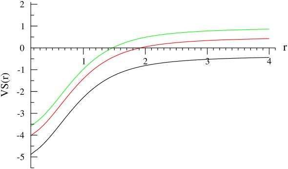
Figure 1: VS(r) for different values of $K^{2}$.

At this point it is convenient to recall that, as explained in section two, the full model, considering its UV completion is not dual to a non-abelian gauge theory, but to a little string theory. Indeed, in the UV, due to the divergent dilaton, the solution has to be S-dualized yielding a IIB solution with NS five branes. In the decoupling limit this background is not dual to ${\cal N}=1$ SYM in four dimensions but to a higher dimensional, 5+1, little string theory. Naturally, trying to calculate observables by simply using the solution up to infinity might not yield sensible answers. In what follows we want to study the glueball spectrum and, if necessary, propose a regularization procedure.

To calculate the $0^{++}$ mass we have to numerically find eigenvalues satisfying equation and appropriate boundary conditions. The asymptotic behavior of the potential is,

$$VS(r\rightarrow\infty)=-\frac{92}{5}+K^{2}$$ (3.32)

$$VS(r\rightarrow 0)=-\frac{1036}{45}+K^{2}$$ (3.33)

Choosing the exponentially decreasing solution at infinity we get,

$${\cal F}(r\rightarrow\infty)\sim e^{-\sqrt{-\frac{92}{5}+K^{2}}r}.$$ (3.34)

At the origin we demand a smooth solution,

$$\frac{dF(r)}{dr}=0.$$ (3.35)

Similarly to Klebanov-Strassler, satisfying the boundary conditions implies that the eigenvalues are bounded from below, $K^{2}>92/5$ and thus, there is a mass gap. But here, in addition of being bounded from below, the eigenvalues are also bounded from above, $K^{2}<1036/45$. A similar phenomenon was observed in [40] in the context of non-commutative gauge theories.

Another difference with the Klebanov-Strassler model is that here the boundary condition at infinity depends on the eigenvalue. In a technical sense, each eigenvalue defines a different problem -different boundary condition- and the spectrum is then given by the eigenvalues of this collection of problems; It is a more general situation than the standard eigenvalue problem.

Using the WKB method [15] we can estimate the eigenvalues $K^{2}$ for which there exists a solution of (3.30) satisfying (3.34) and(3.35). Also, it can be shown numerically that the WKB integral $\int_{0}^{r({\small K^{2}})}{\sqrt{-VS(r)}}dr$ is a monotonically decreasing function of $K^{2}$. And this fact can be used to prove that there is only one eigenvalue in the spectrum. We find, $K_{0}=4.33\ (1/\sqrt{g_{s}\alpha^{\prime}N})$. However, it is easy to show that this eigenvalue does not correspond to a normalizable state. For large r, $\sqrt{{\rm det}\ g}\sim e^{\frac{5}{2}r}$ and thus,

$$\sqrt{{\rm det}g}{\cal F}_{0}^{2}\sim e^{(\frac{5}{2}-2\sqrt{(-\frac{92}{5}+4.3^{2})}r})$$ (3.36)

so the integral $\int_{0}^{\infty}\sqrt{{\rm det}g}{\cal F}_{0}^{2}$ does not converge. The issue we are confronted with now is to find a good regularization for this model.

Let us note an important point. Sean Hartnoll pointed that one might think of taking the norm in flat space $\int dr|{\cal F}|^{2}$. Indeed, the equation (3.30) seems to indicate that, but we used a norm obtained from on the ten dimensional curved background $\int d^{10}x|{\cal F}|^{2}$, and is this norm the one that is forcing us to some regularization. His comment is based on the fact that one should only worry about our fluctuations to have finite energy and according to the paper [41], this condition implies the finitness of the norm in flat space. If we use his proposal, our wave functions ${\cal F}(r)$ are normalizable. In this paper we choose to attach to the more conventional norm defined in the curved space. The differences and physical implications of each choice of norm will be investigated elsewhere.

Coming back to the regularization we need to introduce, let us recall the reader that, as explained in section two, in addition to the solution given by (2.1)-(2.8) there is another solution to the BPS equations, that we aluded to as the ”abelian” solution. The abelian (singular) and non-abelian (non-singular) solutions are the same at infinity but the abelian solution is singular in the IR and thus is not a good dual to SYM, that has nothing singular. We propose that a good regularization for this model is to use the background presented in (2.1)-(2.8) up to the point where it becomes indistinguishable from the abelian one. After this point the two solutions are the same and neither of them is dual to SYM, but to a higher dimensional theory on which we are not interested here.

Figure (2) shows a plot of the Schrödinger potential for the abelian and non abelian solutions. Our proposal is that the IR solution that captures the physics of N=1 SYM is valid only up to the region $\Lambda_{Ab}$ where the potential becomes the same as the one of the abelian solution. The scale $\Lambda_{Ab}$, measured in units of $g_{s}\alpha^{\prime}N$, is set by the vacuum expectation value of the dilaton $\Phi_{0}$.

Numerically we are not doing anything new; the choice of the right endpoint of integration is always arbitrary, decided to best fit the physical problem at hand. Using a generalized shooting technique and integrating up to the point where $V_{Ab}=V_{NonAb}\pm 0.00001$, we find an improved value for the WKB estimate, $K_{0}=4.291(1/\sqrt{g_{s}\alpha^{\prime}N})$. This is a numerically stable eigenvalue meaning that small changes in the initital guess or pushing the endpoint of integration further to the right do not afect the value obtained. But this eigenstate is not normalizable, to obtain a normalizable state we have to impose the regularization procedure proposed above. This will be explained in detail in the next section.

It is worth emphasizing that this model produces a discrete spectrum even without any kind of regularization.

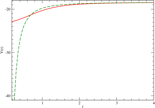
Figure 2: VS(r) for abelian and non-abelian theories, dashed line and solid lines.

3.1 Understanding The Regularization Procedure

Above we have proposed that the correct way of computing in this model is to do a computation with the non-singular solution and, for large values of the radial coordinate, substract the result obtained with the singular background. This, we proposed is calculating in the dual N=1 SYM theory.

Let us get a better intuition of this sort of “regularization procedure”. In physical terms, this procedure is easy to understand and is just instructing us to do our computations only in the region that is of interest to $N=1$ SYM.

Indeed, since the non-abelian (non-singular) solution (that captures the IR effects of the dual field theory) asymptotes to the abelian (singular) solution (that is dual to a higher dimensional field theory), what we are basically doing when explicitely computing is substract the result obtained with the non-singular background minus those obtained at large values of the radial coordinate. Basically, this boils down to computing only in the region that is dual to $N=1$ SYM (with KK impurities as explained above). This is not very different from the type of regularizations done, for example in the computation of Wilson loops [16],[17], where the infinite mass of the non-dynamical quark was substracted, or, what is the same, the mass of an infinite string not feeling the effects of the background (to which the real string asymptotes) is substracted. This sort of regularization was also used in [20]. In that paper, even when a hard cut-off was imposed for numerical convenience, one should think about it as the fact that the computation was done in the region of interest, where the probe brane that adds flavor to the quenched version of N=1 SQCD is different from the probe brane in the singular background. More recently this sort of regularization was used in [24], even when the model used in that paper is different from ours, we believe their regularization can be understood in the lines we wrote above.

Some readers might object the following: if one computes in this way, everything will give a finite result, so in this case, all functions will be normalizable. This questioning is valid, so let us try to answer it; for this it will be convenient to resort on an example where an exact solution is known.

Hence, it is instructive to analyze the solution studied in the paper [13]. Indeed, in that paper, the authors realized that a fluctuation given by

$$\delta g_{\mu\nu}=\delta\phi=0,\;\;\;\delta F_{3}.F_{3}=0,\;\;\delta F_{3}=*_{4}dA_{2}$$ (3.37)

with no restrictions to the functional form of the two form, solves the eqs of motion, that are written in the Appendix B (B.1)-(B.8). This could be a massless glueball, but when computing the norm

$$\int d^{10}x\sqrt{g}|\delta F_{3}|^{2},$$

seems to diverge, thus ruling it out as an state in the strong coupling theory.

If we apply our criteria to this case, one might worry that the norm computed above will give a finite result, thus leading to a massless glueball that one does not expect in this theory (contrary to the KS case [13]). If these quantities give a finite result, this will imply that an effect not expected (a massless glueball) shows up.

So, to understand this, let us do the computation for the norm, and apply our regularization procedure

$$||\delta F_{3}||\propto\int dre^{2h+2\phi}$$ (3.38)

the regularization proposed above, indicates that we do a computation like this

$$||\delta F_{3}||=\int_{0}^{r_{0}}dre^{2\phi+2h}|_{non-singular}+\int_{r_{0}}^{\infty}dre^{2\phi+2h}|_{non-singular}-\int_{r_{0}}^{\infty}dre^{2\phi+2h}|_{singular}$$ (3.39)

Where $r_{0}$ is a value of the radial coordinate where the functions $e^{2h+2\phi}$ computed in the singular and non-singular backgrounds are very similar to some degree of precision that is arbitrarily fixed. Since both integrands have the same asymptotics, they should equally diverge at large values of the radial coordinate. Indeed, both integrals diverge at leading order in the same way, but contrary to what one might expect, the integrals differ in a divergent quantity (and many convergent terms), thus, the computation in (3.39) is divergent and the configuration in (3.37) is not a good state of our theory.

It is important to observe that many of the test that the solution has passed (see the review articles [23] ), still work with this regularization.

We would like to stress that even what was done in [14] was not technically correct (as we mentioned, they seem to have used the wrong fluctuated eqs), the hard cut-off that they introduced is doing the same job that the regularization that we proposed here. Nevertheless, we have to make clear some important differences with [14] (apart from the fact that we use different eqs.). In [14] the authors did not find a discrete spectrum before imposing their hard cut-off, while we found one before our regularization, notice that our potential $VS(r)$ does ‘confine’ wavefunctions. We need to appeal to the regularization, only to satisfy the normalizability condition of our discrete states (and this is because we are being conservative and adopting a curved space measure for our normalizations). So, the hard cut-off regulation is quite different from what we have done here. If one introduces a cut-off, together with some boundary conditions, all solutions to the Schroedinger eqs will be normalizable. In our case, things are more subtle, as we explained above.

4 Glueballs from type IIA perspective

This sections uses the same methods developed in Section 3 (See Appendix B.2 for all the details) for the type IIA background explained in Section 2. We will not carry out a full numerical analysis like in Section 3, but we will leave the system set for this more complicated (fully numerical) problem.

Let us study glueballs for the case of wrapped branes in type IIA string theory. As explained above, in this case, the relevant background consists in $N$ D6 branes wrapping a three cycle inside a CY3 fold. So, to summarize the things clearly, let us write the dilaton and the metric of the IIA solution in Einstein frame,

$$ds_{E}^{2}=2e^{\phi/6}\Big{(}dx_{1,3}^{2}+dr^{2}+(b(r)^{2}+g(r)^{2})(d\theta^{2}+\sin^{2}\theta d\varphi^{2})+a(r)^{2}(d\tilde{\theta}^{2}+\sin^{2}\tilde{\theta}d\tilde{\varphi}^{2})+$$

$$+2g(r)a(r)^{2}[\cos\hat{\psi}(d\theta d\tilde{\theta}+\sin\theta\sin\tilde{\theta}d\varphi d\tilde{\varphi})+\sin\hat{\psi}(\sin\theta d\tilde{\theta}d\varphi-sin\tilde{\theta}d\theta d\tilde{\varphi})]+$$

$$+\frac{f^{2}c^{2}}{f^{2}+c^{2}(1+g_{3})^{2}}(d\hat{\psi}+\cos\theta d\varphi-\cos\tilde{\theta}d\tilde{\varphi})^{2}\Big{)},$$

$$4e^{4/3\phi}=f(r)^{2}+c(r)^{2}(1+g_{3}(r))^{2}.$$ (4.40)

The field strength $F_{2}$ reads,

$$F_{2}=k^{\prime}(r)dr\wedge(d\hat{\psi}+\cos\theta d\varphi-\cos\tilde{\theta}d\tilde{\varphi})-(k(r)+1)\sin\theta d\theta\wedge d\varphi+(k(r)-1)\sin\tilde{\theta}d\tilde{\theta}\wedge d\tilde{\varphi},$$ (4.41)

with

$$k(r)=\frac{f^{2}-c^{2}(1-g_{3}^{2})}{f^{2}+c^{2}(1+g_{3})^{2}}.$$

In the following, we will work with this IIA set-up and because of the many similarities with the IIB model studied in the previous section, we will use the same approach. It is interesting to mention that if we can find glueballs in IIA, they should have an expression in M theory purely in terms of a metric fluctuation. Let us start by finding the dynamics of the fluctuations. The Lagrangian of IIA is

$$L=\sqrt{g}\Big{(}R-\frac{1}{2}(\partial\phi)^{2}-\frac{1}{4}e^{3/2\phi}F_{2}^{2}-\frac{1}{12}e^{-\phi}H_{3}^{2}-\frac{1}{48}e^{\phi/2}\hat{F}_{4}^{2}\Big{)}+\frac{1}{2}B_{2}\wedge F_{4}\wedge F_{4},$$

$$\hat{F}_{4}=dC_{3}-H_{3}\wedge A_{1},\;\;F_{2}=dA_{1},\;\;H_{3}=dB_{2},$$ (4.42)

now, let us focus on the configurations that are of our interest, that is those where only the fields $\phi,\;g_{\mu\nu},\;A_{\mu}$ are turned on. The eqs of motion in this case are

$$R_{\mu\nu}=\frac{1}{2}\partial_{\mu}\phi\partial_{\nu}\phi+\frac{1}{2}e^{3/2\phi}(F_{\mu*}F_{\nu}^{*}-\frac{1}{16}g_{\mu\nu}F^{2}),$$

$$R=\frac{1}{2}(\partial\phi)^{2}+\frac{3}{16}e^{3/2\phi}F^{2},\;\;\nabla^{2}\phi=\frac{3}{8}e^{3/2\phi}F^{2},$$

$$\partial_{\mu}\Big{(}\sqrt{g}e^{3/2\phi}F^{\mu\nu}\Big{)}=0,\;\;\partial_{[\mu}F_{\nu\rho]}=0$$ (4.43)

Now, let us study the variations of these eqs. Under a fluctuation in all the relevant fields

$$\phi=\phi+\epsilon\delta\phi,\;\;\;g_{\mu\nu}=g_{\mu\nu}+\epsilon h_{\mu\nu}\;\;\;F_{\mu\nu}=F_{\mu\nu}+\epsilon\delta F_{\mu\nu}.$$ (4.44)

Again, we will propose a particular form for the metric fluctuation

$$h_{ij}=\frac{\lambda}{5}hg_{ij},(i,j=x,t,r)\;\;\;h_{\alpha\beta}=h_{(\alpha\beta)}+\frac{h}{5}g_{\alpha\beta}.$$ (4.45)

The same comments that we made regarding this decomposition, before eq. (3.25) are also pertinent here. We have denoted the trace of the internal part of the metric as $h=h_{a}^{a}$. We also propose an armonic expansion for the fields of a form similar to (3.26).

$$h(x,y)=\Sigma_{I}h^{I}(x)Y^{I}(y),\;\;h_{(\alpha\beta)}=\Sigma_{I}b^{I}_{(\alpha\beta)}(x)Y^{I}(y),\;\;\delta\phi(x,y)=\Sigma_{I}f^{I}(x)Y^{I}(y)$$ (4.46)

Keeping only the s-wave fluctuations as before, we find after many computations (that are carefully spelled out in Appendix B), that like in IIB case, the many equations nicely combine and is sufficient to solve just one equation that reads,

$$\nabla^{2}h^{I}+6g^{rr}\partial_{r}\phi\partial_{r}h^{I}+\frac{e^{3/2\phi}}{8}\Big{(}31F^{2}+57(g^{\alpha\beta}F_{\alpha*}F_{\beta}^{*}-\frac{71}{57}g^{rr}F_{r*}F_{r}^{*})\Big{)}h^{I}=0$$ (4.47)

As we have done in the type IIB section, the numerics in this case can be studied. We will not do this here and we just want to point to the fact that even when this has to be done in a completely numerical way (since the metric functions are only numerically known), there is a nice feature of this IIA solution. The fact that the dilaton does not diverge, makes us believe that the regularization will not be necessary. This is left for future work. The point of this section was just to call the reader’s attention to this set of IIA models and show the analogy with the IIB treatment.

5 Summary, Conclusions and Future Directions

Let us start by summarizing what we have done in this paper. First, we presented two Supergravity backgrounds (one in IIB and another in IIA) that are argued to be dual to $N=1$ SYM at low energies and we analyzed the spectrum in detail. Then, we initiated the study of glueball-like excitations in the strong coupling field theory as fluctuations of the Supergravity fields.

We presented the equations to study the spectrum of glueballs and their excitations and analyzed them numerically. The type IIB case is analyzed in detail and we proposed a regularization procedure that might be useful in other computations involving these wrapped branes set-ups. Two appendixes present our computations in full detail.

We find that unlike some IIB backgrounds previously studied, in the D5 wrapped on $S^{2}$ model not even the simplest scalar mode decouples from the rest of the fluctuations. Indeed, as we have shown, assuming only fluctuations of the dilaton leads to inconsistent equations. Therefore, the glueball $0^{++}$ in the IIB model we studied, is not dual to the dilaton, but to a mixture of dilaton and trace of the internal part of the metric. This goes in the same line as the papers [8], where the glueballs turned out to be mixings between different Supergravity modes. This mixing might persist for higher spin modes. The presence of a non-constant dilaton background seems to be the reason for the mixing of the fluctuations and this also appears in the model studied in [42]. Another important point is that the potential found produces a discrete spectrum and a mass gap without any sort of cut-off, which seems to indicate that it is indeed capturing the physics of a confinig theory. As expected in a background with a linear dilaton, the states are not normalizable. Given that the UV completion of this theory is a little string theory it is not a surprise that a regularization (or substraction) procedure is needed. We present a proposal for this regularization which amounts to substracting the unwanted contribution of the UV regime.

In the analysis of the type IIA background, we find that the scalar mode does not decouple from the rest of the fluctuations, indicating that, indeed, the non-constant dilaton in the background plays a role in producing this mixing. We do not perform the numerical analysis of the IIA background since the point of the paper is more to show a way of proceeding in these wrapped brane set-ups, that we believe is not exploited in the previous literature.

Let us now discuss some future directions to follow and some work that should be interesting to do in detail, not discussed in this paper.

First of all, as we mentioned in section 2, these models are contamined by the so called KK modes and we do not distinguish here if the glueballs we are obtaining are actually “made out” of KK modes composites (in which case they are not proper “glueballs” but hybrids composed of gluon, gluino and KK state)

A good technical way to distinguish is to repeat the computation we are doing in Section 3, but for the case of the “dipole deformed” field theory (see [43] for all details). Indeed, the idea in the paper [43] is to make a $SL(3,R)$ deformation of the supergravity solution, that reflects on the dual field theory side on particular deformation that affects only the dynamics of the KK modes in the spectrum. Hence, the comparison of the eqs (3.27) and those in the appendix with those obtained in using the deformed metric can illuminate on what type of composition our ‘glueball’ has, if only glue and gluino, or if it is composed out of KK modes. Same could be repeated with deformations of the $G_{2}$ holonomy manifolds and the many examples already existing in the literature.

It would be nice to check how our regularizing procedure works with the “flavor branes” introduced in [20] when doing a dual to quenched SQCD. Indeed, there the idea was precisely the same, taking away from the computation the effects of the unwanted UV region. This can be understood by looking at the plots in figures 2 and 3 of [20].

It should also be of interest, to study the glueballs in the type IIA model discussed in Section 4.1 of the paper [44]. This solution is basically the same as the one we discussed in the IIB section, after some dualities. So, the interest of studying glueballs in this case is obviously to see if the same spectrum is obtained, analyze differences among eqs of motion, etc.

Besides, it might have some interest to study the IIA case in more detail, not only numerically, as we pointed out above, but also from a $G_{2}$ holonomy perspective. Our dilaton-metric-gauge field fluctuations must combine in some way in a pure metric fluctuation in eleven dimensions. It should be nice to see how this works.

Other models where it might have be interesting to apply our techniques (mainly the sort of manipulations explained in the Appendix B) is in models of non-supersymmetric duality. There is indeed one very clear model, that was studied in detail in the papers [45].

One might also think about studying the ‘fermionic counterpart’ of what we have done in this paper, by fluctuating the fermionic fields around the bosonic background.

On other respect, the comparison with the results from Lattice SYM should be done. There are some of these results in but we believe that the topic will evolve to allow better understanding and the contribution of this paper might be useful in the comparison with lattice results. See for example[46]. Regarding this point, it should be interesting to study the spectrum of fermionic fluctuations (with fermionic fields vanishing in the background). This does not seem to have been exploited in the AdS/CFT literature, while other methods based on Veneziano-Yankielowicz and extensions, seem to give nice results [46]. This situation might clearly improve with some study.

The interest of studying glueballs goes beyond the simple fact of getting a discrete spectrum (that is by itself of enough interest). Indeed, glueballs play an important role in some recent advances regarding the study of Deep Inelastic and other types of Scattering using AdS/CFT techniques [47]. The knowledge of glueballs masses and profiles in different models might help to extend the results in papers like [47] to other ‘more realistic’ models.

6 Acknowledgments:

We thank Richard Brower, José Edelstein, Nick Evans, Sean Hartnoll, Rafael Hernández, Oliver Jahn, Martin Kruczenski, Juan Martin Maldacena, Alfonso Ramallo, Angel Paredes, Chung-I-Tan, Pere Talavera and Stathis Tompaidis for discussions and comments that helped improving the presentation and interest of the results of this paper. Elena Cáceres would like to thank the Theory Group at the University of Texas at Austin for hospitality during the final stages of this work. This work was supported in part by the National Science Foundation under Grant No. PHY-0071512 and PHY-0455649, the US Navy, Office of Naval Research, Grant Nos. N00014-03-1-0639 and N00014-04-1-0336, Quantum Optics Initiative and by funds provided by the U.S.Department of Energy (DoE) under cooperative research agreement DF-FC02-94ER408818. Elena Cáceres is also supported by Mexico’s Council of Science and Technology, CONACyT, grant No.44840. Carlos Nuñez is a Pappalardo Fellow.

Appendix A Appendix: Some Geometrical identities

In the following, we list some geometrical identities that were used in the derivation of the fluctuated eqs (B.5)-(B.8)

$$\delta R=\nabla_{\mu}\nabla_{\nu}h^{\mu\nu}-\nabla^{2}h_{\mu}^{\mu}-R_{\mu\nu}h^{\mu\nu},$$

$$\delta R_{\mu\nu}=\frac{1}{2}[\nabla_{\alpha}\nabla_{\mu}h_{\nu}^{\alpha}+\nabla_{\alpha}\nabla_{\nu}h_{\mu}^{\alpha}-\nabla_{\nu}\nabla_{\mu}h_{\alpha}^{\alpha}-\nabla^{2}h_{\mu\nu}],\;\;\sqrt{g+h}=\sqrt{g}(1+\frac{\epsilon}{2}h_{\mu}^{\mu})+O(\epsilon^{2}),$$

$$\delta\Gamma_{\mu\nu}^{\lambda}=\frac{1}{2}g^{\alpha\lambda}(\nabla_{\mu}h_{\alpha\nu}+\nabla_{\nu}h_{\alpha\mu}-\nabla_{\alpha}h_{\mu\nu})\rightarrow g^{\alpha\beta}\delta\Gamma_{\alpha\beta}^{r}=-\frac{1}{2}g^{rr}(\nabla_{r}h_{\mu}^{\mu}-2\nabla_{\mu}h_{r}^{\mu})$$

$$\delta(\nabla^{2}\phi)=\nabla^{2}\delta\phi-g^{ab}\delta\Gamma_{ab}^{\rho}\partial_{\rho}\phi-h^{ab}\nabla_{a}\nabla_{b}\phi$$ (A.1)

Appendix B Appendix: Derivation of the eqs in the IIB and IIA cases

In this Appendix we fill in all the details that were left out in the computations that lead to eqs. (3.27) and (4.47) in sections three and four.

B.1 Glueballs with the D5 branes solution

Let us start with the type IIB solution. To study glueballs, we need the variation of the eqs of motion. In the type IIB case, for the solution of D5 branes wrapping $S^{2}$, the Einstein eqs for the metric, dilaton and three form read,

$$R_{\mu\nu}=\frac{1}{2}\partial_{\mu}\phi\partial_{\nu}\phi+\frac{g_{s}e^{\phi}}{4}\Big{(}F_{\mu**}F_{\nu}^{**}-\frac{1}{12}g_{\mu\nu}F_{3}^{2}\Big{)}$$ (B.1)

by contracting we get the Ricci scalar eq,

$$R=\frac{1}{2}(\partial_{\mu}\phi)^{2}+\frac{g_{s}e^{\phi}}{24}F_{3}^{2}.$$ (B.2)

The dilaton, Maxwell and Bianchi eqs. are,

$$\nabla^{2}\phi=\frac{g_{s}e^{\phi}}{12}F_{3}^{2},\;\;\partial_{\mu}\Big{(}\sqrt{g}e^{\phi}F^{\mu\nu\rho}\Big{)}=0,\;\;\partial_{[\mu}F_{\kappa\nu\rho]}=0$$ (B.3)

Now, let us study the fluctuations of these eqs. above. Let us assume that the background fields vary according to

$$g_{\mu\nu}\rightarrow g_{\mu\nu}+\epsilon h_{\mu\nu},\;\;\phi\rightarrow\phi+\epsilon\delta\phi,\;\;F_{\mu\nu\rho}\rightarrow F_{\mu\nu\rho}+\epsilon\delta F_{\mu\nu\rho}$$ (B.4)

So, keeping only linear order in the parameter $\epsilon$, we get eqs for the fluctuated fields that read, for variation in the Ricci tensor eq. (3.21),

$$\frac{1}{2}[\nabla_{\alpha}\nabla_{\mu}h_{\nu}^{\alpha}+\nabla_{\alpha}\nabla_{\nu}h_{\mu}^{\alpha}-\nabla_{\nu}\nabla_{\mu}h_{\alpha}^{\alpha}-\nabla^{2}h_{\mu\nu}]=\frac{1}{2}[\partial_{\mu}\phi\partial_{\nu}\delta\phi+\partial_{\mu}\delta\phi\partial_{\nu}\phi]$$

$$+\frac{g_{s}e^{\phi}}{4}[\delta\phi F_{\mu**}F_{\nu}^{**}+\delta F_{\mu**}F_{\nu}^{**}+F_{\mu**}\delta F_{\nu}^{**}-2h^{ab}F_{\mu a*}F_{\nu b}^{*}]$$

$$-\frac{g_{s}e^{\phi}}{48}[g_{\mu\nu}(2F_{3}\delta F_{3}-3h^{ab}F_{a**}F_{b}^{**}+\delta\phi F_{3}^{2})+h_{\mu\nu}F_{3}^{2}]$$ (B.5)

and for the Ricci scalar eq.(B.2)

$$\nabla_{\mu}\nabla_{\nu}h^{\mu\nu}-\nabla^{2}h_{\mu}^{\mu}-R_{\mu\nu}h^{\mu\nu}=g^{\mu\nu}\partial_{\mu}\phi\partial_{\nu}\delta\phi-\frac{h^{\mu\nu}}{2}\partial_{\mu}\phi\partial_{\nu}\phi+$$

$$\frac{g_{s}e^{\phi}}{24}[2F_{3}\delta F_{3}-3h^{kl}F_{k**}F_{l}^{**}+\delta\phi F_{3}^{2}],$$ (B.6)

For the fluctuated dilaton eq. we have,

$$\nabla^{2}\delta\phi-h^{\mu\nu}\nabla_{\mu}\partial_{\nu}\phi-\frac{1}{2}g^{rr}\partial_{r}\phi(2\nabla^{\mu}h_{r\mu}-\partial_{r}h_{\mu}^{\mu})-\frac{g_{s}e^{\phi}}{12}(\delta\phi F^{2}+2F\delta F-3h^{\mu\nu}F_{\mu**}F_{\nu}^{**})=0$$ (B.7)

and for the fluctuation of the Maxwell eq. and Bianchi identity,

$$\partial_{\mu}[\sqrt{g}e^{\phi}((\frac{1}{2}h_{\rho}^{\rho}+\delta\phi)F^{\mu\nu\alpha}+\delta F^{\mu\nu\alpha}-h^{\alpha c}F^{\mu\nu}_{c}+h^{\nu c}F^{\mu\alpha}_{c}-h^{\mu c}F_{c}^{\nu\alpha})]=0,\;\;d\delta F=0$$ (B.8)

Notice that the Ricci scalar eq. (B.6) can be obtained by contracting the Ricci tensor eq. (B.5) and substracting $h^{\mu\nu}R_{\mu\nu}$, so, in the following we will work with a contracted version of (B.5). In the derivation of these eqs, we have used the geometrical identities reviewed in Appendix A.

Now, let us assume a fluctuation for the metric of the form

$$h_{ij}=\frac{\lambda}{5}g_{ij}h^{\alpha}_{\alpha},\;\;(i,j=\vec{x},t,r)$$

$$h_{\alpha\beta}=h_{(\alpha\beta)}+\frac{1}{5}g_{\alpha\beta}h^{a}_{a},\;\;(\alpha\beta)=(\theta,\tilde{\theta},\varphi,\tilde{\varphi},\psi)$$ (B.9)

Where $\lambda$ is a constant and we have performed a shift in the $h_{\alpha\beta}$, this shift is proportional to the trace of the internal part of the metric $h^{\alpha}_{\alpha}$. Note that the trace of the metric fluctuation over all the space is, $h^{\mu}_{\mu}=(\lambda+1)h^{\alpha}_{\alpha}$. Now, let us study the form of the fluctuation of the eq. that is obtained by contracting (B.5) with the background metric $g^{\mu\nu}\delta R_{\mu\nu}$,

$$\nabla_{\mu}\nabla_{\nu}h^{\mu\nu}-\nabla^{2}h_{\mu}^{\mu}=\partial^{r}\delta\phi\partial_{r}\phi+\frac{g_{s}e^{\phi}}{24}[(\delta\phi-\frac{1}{2}g^{\mu\nu}h_{\mu\nu})F_{3}^{2}+3h^{\rho\sigma}F_{\rho**}F_{\sigma}^{**}+2\delta F_{3}\cdot F_{3}]\\$$ (B.10)

and using (B.9),

$$\frac{1}{5}\lambda\nabla^{2}_{x}h^{\alpha}_{\alpha}-(\lambda+1)(\nabla^{2}_{x}+\nabla^{2}_{y})h^{\alpha}_{\alpha}-g^{rr}\partial_{r}\delta\phi\partial_{r}\phi-\frac{g_{s}e^{\phi}}{24}\Big{[}(\delta\phi-\frac{(\lambda+1)}{2}h^{\alpha}_{\alpha})F_{3}^{2}$$

$$+\frac{3}{5}(\lambda g^{rr}F_{r**}F_{r}^{**}+g^{ab}F_{a**}F_{b}^{**})h_{\alpha}^{\alpha}+2F_{3}\delta F_{3}+3h^{(ab)}F_{a**}F_{b}^{**}\Big{]}=0.$$ (B.11)

For the dilaton eq. (B.7) we will have,

$$\nabla^{2}\delta\phi+(\frac{3\lambda+5}{10})g^{rr}\partial_{r}\phi\partial_{r}h_{\alpha}^{\alpha}-\frac{g_{s}e^{\phi}}{12}\Big{[}(\delta\phi+\frac{\lambda}{5}h_{\alpha}^{\alpha})F^{2}+2F_{3}\delta F_{3}-$$

$$-\frac{3}{5}h_{\alpha}^{\alpha}(\lambda g^{rr}F_{r**}F_{r}^{**}+g^{ab}F_{a**}F_{b}^{**})-4h^{(\alpha\beta)}F_{\alpha**}F_{\beta}^{**}\Big{]}$$ (B.12)

We have used the eq. of motion for the dilaton in the background eq.(3.23) above. The next step is to introduce an expansion in harmonics for each of the fields

$$h^{\alpha}_{\alpha}(x,y)=\Sigma_{I}\Pi^{I}(x)Y^{I}(y),\;\;h_{(\alpha\beta)}=\Sigma_{I}b^{I}(x)Y^{I}_{(\alpha\beta)}(y),\;\;\delta\phi(x,y)=\Sigma_{I}f^{I}(x)Y^{I}(y)$$ (B.13)

In order to satisfy the Bianchi identity we write the fluctuation $\delta F_{3}$ in the form

$$\delta F_{\mu\nu\rho}=\partial_{[\mu}\delta A_{\nu\rho]}$$ (B.14)

We will show that it is possible to find a fluctuation $\delta F_{3}$ orthogonal to the background $F_{3}$, i.e $\delta F_{3}\cdot F_{3}=0$, that satisfies Maxwell’s equation.

Let us write the different componentes of Maxwell’s equation for a general fluctuation $\delta F_{3}=\partial_{[\mu}\delta A_{\nu\rho]}$ without demanding yet orthogonality with the backgorund $F_{3}$. We get

$\bullet\nu,\alpha=a,b$ (angular)

$$\partial_{r}[\sqrt{g}e^{\phi}((\frac{1}{2}h_{\mu}^{\mu}+\delta\phi)F^{rab}+\partial^{[r}\delta A^{ab]}-h^{bc}F^{ra}_{c}+h^{ac}F^{rb}_{c}-h^{rc}F_{c}^{ab})]$$

$$+\partial_{\theta}[\sqrt{g}e^{\phi}((\frac{1}{2}h_{\mu}^{\mu}+\delta\phi)F^{\theta ab}+\partial^{[\theta}\delta A^{ab]}-h^{bc}F^{\theta a}_{c}+h^{ac}F^{\theta b}_{c}-h^{\theta c}F_{c}^{ab})]+\partial_{x}[\sqrt{g}e^{\phi}(\partial^{[x}A^{ab]})]=0$$

. (B.15)

$\bullet\nu,\alpha=r,b$ (r,angular)

$$\partial_{\theta}[\sqrt{g}e^{\phi}((\frac{1}{2}h_{\mu}^{\mu}+\delta\phi)F^{\theta rb}+\partial^{[\theta}\delta A^{rb]}-h^{bc}F^{\theta r}_{c}+h^{rc}F^{\theta b}_{c}-h^{\theta c}F_{c}^{rb})]+\partial_{x}[\sqrt{g}e^{\phi}(\partial^{[x}\delta A^{rb]})]=0$$

. (B.16)

$\bullet\nu,\alpha=yz$

$$\partial_{r}[\sqrt{g}e^{\phi}(\partial^{[r}\delta A^{yz]})]+\partial_{\theta}[\sqrt{g}e^{\phi}(\partial^{[\theta}A^{yz]})]+\partial_{x}[\sqrt{g}e^{\phi}(\partial^{[x}\delta A^{yz]})]=0.$$ (B.17)

$\bullet\nu,\alpha=(r,z)$

$$\partial_{\theta}[\sqrt{g}e^{\phi}(\partial^{[\theta}A^{rz]})]+\partial_{x}[\sqrt{g}e^{\phi}(\partial^{[x}\delta A^{rz]})]=0.$$ (B.18)

Now demand $\delta F_{3}\cdot F_{3}=0$, thus $\delta F_{rab}=\delta F_{\theta ab}=0$. From equations (B.15) and (B.16) above it is clear that a fluctuation of the form

$$-\partial_{x}[\sqrt{g}e^{\phi}(\partial^{[x}A^{ab]})] = \partial_{r}[\sqrt{g}e^{\phi}((\frac{1}{2}h_{\mu}^{\mu}+\delta\phi)F^{rab}-h^{bc}F^{ra}_{c}+h^{ac}F^{rb}_{c}-h^{rc}F_{c}^{ab})]$$

$$+ \partial_{\theta}[\sqrt{g}e^{\phi}((\frac{1}{2}h_{\mu}^{\mu}+\delta\phi)F^{\theta ab}-h^{bc}F^{\theta a}_{c}+h^{ac}F^{\theta b}_{c}-h^{\theta c}F_{c}^{ab})]$$

$$-\partial_{x}[\sqrt{g}e^{\phi}(\partial^{[x}\delta A^{rb]}) = \partial_{\theta}[\sqrt{g}e^{\phi}((\frac{1}{2}h_{\mu}^{\mu}+\delta\phi)F^{\theta rb}-h^{bc}F^{\theta r}_{c}+h^{rc}F^{\theta b}_{c}-h^{\theta c}F_{c}^{rb})]$$

with the other components given by (B.17) and (B.18) will satisfy Maxwell’s equation, the Bianchi identity and is such that $\delta F_{3}\cdot F_{3}=0$.

Therefore, we have only eqs. (B.11) and (B.12), that keeping only the S-wave in the expansion in harmonics (B.13) take the form,

$$-(\frac{4\lambda}{5}+1)\nabla^{2}_{x}\Pi(x)-\partial^{r}f(x)\partial_{r}\Phi-\frac{g_{s}e^{\phi}}{24}\Big{[}(f(x)-\frac{(\lambda+1)}{2}\Pi(x))F_{3}^{2}$$

$$+\frac{3}{5}(\lambda g^{rr}F_{r**}F_{r}^{**}+g^{ab}F_{a**}F_{b}^{**})\Pi(x)\Big{]}=0$$ (B.20)

and

$$\nabla^{2}f(x)+(\frac{3\lambda}{10}+\frac{1}{2})\partial^{r}\Pi(x)\partial_{r}\Phi-\frac{g_{s}}{12}e^{\phi}\Big{[}(f(x)+\frac{\lambda}{5}\Pi(x))F_{3}^{2}-$$

$$\frac{3}{5}(g^{ab}F_{a**}F_{b}^{**}+\lambda g^{rr}F_{r**}F_{r}^{**})\Pi(x)\Big{]}=0$$ (B.21)

Equations (B.20) and (B.21) look suggestively similar so we will first check if there is any value of $\lambda$ for which they are the same. Indeed, for the two equations to be equal we need to satisfy

$$2(\frac{4\lambda}{5}+1)\Pi(x)=f(x),\;\;$$

$$2f(x)=(\frac{3\lambda}{10}+\frac{1}{2})\Pi(x),$$

$$-(f(x)-\frac{(\lambda+1)}{2}\Pi(x))=f(x)+\frac{\lambda}{5}\Pi(x)$$ (B.22)

It is easy to check that $\lambda=-\frac{35}{29}$ does the job. The eq. we need to solve is,

$$\nabla^{2}f(x)+2g^{rr}\partial_{r}f(x)\partial_{r}\phi+\frac{g_{s}}{12}e^{\phi}\Big{[}\frac{5}{2}F_{3}^{2}+\frac{29\cdot 3}{10}(g^{ab}F_{a**}F_{b}^{**}-\frac{35}{29}g^{rr}F_{r**}F_{r}^{**})\Big{]}f(x)=0$$ (B.23)

This is precisely the eq.(3.27) we wanted to obtain.

B.2 Glueballs with the D6 branes solution

The relevant background consists in $N$ D6 branes wrapping a three cycle inside a CY3 fold. So,the metric of our IIA solution in Einstein frame and the dilaton where given in (4.40), and the Maxwell Field strength was,

$$F_{2}=k^{\prime}(r)dr\wedge(d\hat{\psi}+\cos\theta d\varphi-\cos\tilde{\theta}d\tilde{\varphi})-(k(r)+1)\sin\theta d\theta\wedge d\varphi+(k(r)-1)\sin\tilde{\theta}d\tilde{\theta}\wedge d\tilde{\varphi},$$ (B.24)

with

$$k(r)=\frac{f^{2}-c^{2}(1-g_{3}^{2})}{f^{2}+c^{2}(1+g_{3})^{2}}.$$

Because of the many similarities with the IIB model studied in previous sections, we will use the same approach. Let us first study fluctuations. The Lagrangian of IIA is

$$L=\sqrt{g}\Big{(}R-\frac{1}{2}(\partial\phi)^{2}-\frac{1}{4}e^{3/2\phi}F_{2}^{2}-\frac{1}{12}e^{-\phi}H_{3}^{2}-\frac{1}{48}e^{\phi/2}\hat{F}_{4}^{2}\Big{)}$$

$$+\frac{1}{2}B_{2}\wedge F_{4}\wedge F_{4},$$

$$\hat{F}_{4}=dC_{3}-H_{3}\wedge A_{1},\;\;F_{2}=dA_{1},\;\;H_{3}=dB_{2}.$$ (B.25)

now, let us focus on the configurations that are of our interest, that is those where only the fields $\phi,\;g_{\mu\nu},\;A_{\mu}$ are turned on. The eqs of motion in this case are

$$R_{\mu\nu}=\frac{1}{2}\partial_{\mu}\phi\partial_{\nu}\phi+\frac{1}{2}e^{3/2\phi}(F_{\mu*}F_{\nu}^{*}-\frac{1}{16}g_{\mu\nu}F^{2}),$$

$$R=\frac{1}{2}(\partial\phi)^{2}+\frac{3}{16}e^{3/2\phi}F^{2},\;\;\nabla^{2}\phi=\frac{3}{8}e^{3/2\phi}F^{2},$$

$$\partial_{\mu}\Big{(}\sqrt{g}e^{3/2\phi}F^{\mu\nu}\Big{)}=0,\;\;\partial_{[\mu}F_{\nu\rho]}=0$$ (B.26)

Now, let us study the variations of these eqs. Under a fluctuation in all the relevant fields

$$\phi=\phi+\epsilon\delta\phi,\;\;\;g_{\mu\nu}=g_{\mu\nu}+\epsilon h_{\mu\nu}\;\;\;F_{\mu\nu}=F_{\mu\nu}+\epsilon\delta F_{\mu\nu}$$ (B.27)

we have to first order in the fluctuation parameter $\epsilon$,

$$\delta R_{\mu\nu}=\frac{1}{2}(\partial_{\mu}\phi\partial_{\nu}\delta\phi+\partial_{\nu}\phi\partial_{\mu}\delta\phi)+\frac{1}{2}e^{3/2\phi}\Big{(}\frac{3}{2}\delta\phi(F_{\mu*}F_{\nu}^{*}-\frac{1}{16}g_{\mu\nu}F^{2})+F_{\mu*}\delta F_{\nu}^{*}+$$

$$F_{\nu*}\delta F_{\mu}^{*}-h^{ab}F_{\mu a}F_{\nu b}-\frac{1}{8}g_{\mu\nu}(F\delta F-h^{\alpha\beta}F_{\alpha*}F_{\beta}^{*})-\frac{1}{16}h_{\mu\nu}F^{2}\Big{)},$$

$$\delta R=g^{\mu\nu}\partial_{\mu}\phi\partial_{\nu}\delta\phi-\frac{h^{\mu\nu}}{2}\partial_{\mu}\phi\partial_{\nu}\phi+\frac{3}{16}e^{3/2\phi}\Big{(}\frac{3}{2}\delta\phi F^{2}+2F\delta F-2h^{\mu\nu}F_{\mu*}F_{\nu}^{*}\Big{)},$$

$$\delta(\nabla^{2}\phi)=\frac{3}{8}e^{3/2\phi}(\frac{3}{2}\delta\phi F^{2}+2F\delta F-2h^{\mu\nu}F_{\mu*}F_{\nu}^{*}),$$

$$\partial_{\mu}\Big{(}\sqrt{g}e^{3/2\phi}[(3\delta\phi+h_{\mu}^{\mu})\frac{F^{\mu\nu}}{2}+\delta F^{\mu\nu}-h^{\nu}_{a}F^{\mu a}-h^{\mu}_{a}F^{\nu a}]\Big{)}=0$$ (B.28)

So, using the geometrical variations given in the Appendix A and putting all together, we end up with three eqs, one for the variation of the dilaton, one for the Ricci scalar and the Maxwell eq. One can see that the eq for the variation of the Ricci tensor is included in the Ricci scalar variation.

So, we have

$$\nabla_{\mu}\nabla_{\nu}h^{\mu\nu}-\nabla^{2}h_{\mu}^{\mu}=g^{\mu\nu}\partial_{\mu}\phi\partial_{\nu}\delta\phi+\frac{e^{3/2\phi}}{8}\Big{(}\frac{9}{4}\delta\phi F^{2}+3F\delta F+h^{\mu\nu}F_{\mu*}F_{\nu}^{*}-\frac{h^{\mu}_{\mu}}{4}F^{2}\Big{)}$$ (B.29)

$$\nabla^{2}\delta\phi-h^{\mu\nu}\nabla_{\mu}\nabla_{\nu}\phi-\frac{g^{rr}}{2}(2\nabla_{\mu}h_{r}^{\mu}-\nabla_{r}h_{\mu}^{\mu})\partial_{r}\phi=\frac{3e^{3/2\phi}}{8}\Big{(}\frac{3}{2}\delta\phi F^{2}+2F\delta F-2h^{\mu\nu}F_{\mu*}F_{\nu}^{*}\Big{)}$$ (B.30)

$$\partial_{\mu}\Big{(}\sqrt{g}e^{3/2\phi}[(3\delta\phi+h_{k}^{k})\frac{F^{\mu\nu}}{2}+\delta F^{\mu\nu}-h^{\nu}_{a}F^{\mu a}-h^{\mu}_{a}F^{a\nu}]\Big{)}=0$$ (B.31)

Now, let us propose a fluctuation of the metric $h_{\mu\nu}$ of the form

$$h_{ij}=\frac{\lambda}{5}hg_{ij},(i,j=x,t,r)\;\;\;h_{\alpha\beta}=h_{(\alpha\beta)}+\frac{h}{5}g_{\alpha\beta}$$ (B.32)

Here, we denote the trace of the internal part of the metric as $h=h_{a}^{a}$. So, let us study the fluctuated eqs, we will have for the Ricci scalar,

$$\Big{(}\frac{(4\lambda+5)}{5}\nabla^{2}_{x}+\frac{(4+5\lambda)}{5}\nabla^{2}_{y}\Big{)}h+g^{rr}\partial_{r}\phi\partial_{r}\delta\phi+\frac{e^{3/2\phi}}{8}\Big{(}[\frac{9\delta\phi-(\lambda+1)h}{4}]F^{2}+3F\delta F$$

$$+\frac{h}{5}(g^{\alpha\beta}F_{\alpha*}F_{\beta}^{*}+\lambda g^{rr}F_{r*}F_{r}^{*})\Big{)}-g^{(\alpha\beta)}(\nabla_{\alpha}\nabla_{\beta}h+F_{\alpha*}F_{\beta}^{*})=0$$ (B.33)

and for the dilaton, after the eq. of motion for the background dilaton field has been used we will have,

$$\nabla^{2}\delta\phi+(\frac{3\lambda+5}{10})g^{rr}\partial_{r}\phi\partial_{r}h-\frac{e^{3/2\phi}}{8}\Big{(}[\frac{9}{2}\delta\phi+\frac{3\lambda}{5}h]F^{2}+6F\delta F-\frac{6}{5}h(g^{\alpha\beta}F_{\alpha*}F_{\beta}^{*}+\lambda g^{rr}F_{r*}F_{r}^{*})$$

$$-\frac{3}{4}g^{(\alpha\beta)}F_{\alpha*}F_{\beta}^{*}\Big{)}=0$$ (B.34)

and the Maxwell eq.

$$\partial_{\mu}\Big{(}\sqrt{g}e^{3/2\phi}[(3\delta\phi+h)\frac{F^{\mu\nu}}{2}+\delta F^{\mu\nu}-\frac{\lambda}{5}g^{\nu r}F^{\mu}_{r}-g^{\nu a}hF^{\mu}_{a}-g^{(\nu a)}F^{\mu}_{a}+$$

$$\frac{\lambda}{5}g^{\mu r}hF^{\nu}_{r}-g^{\mu a}hF^{\nu}_{a}+g^{(\mu a)}F^{\nu}_{a}]\Big{)}=0$$ (B.35)

Now, let us follow an analysis very similar to the one we have done for the Type IIB case. First, we will propose an expansion of the form (B.13).

$$h(x,y)=\Sigma_{I}h^{I}(x)Y^{I}(y),\;\;h_{(\alpha\beta)}=\Sigma_{I}b^{I}(x)Y^{I}_{(\alpha\beta)}(y),\;\;\delta\phi(x,y)=\Sigma_{I}f^{I}(x)Y^{I}(y)$$ (B.36)

Then, let us impose that both eqs are indeed the same. For this to happen, we will also need that the fluctuation of the Maxwell field is orthogonal to the field itself, that is

$$\delta F_{\mu\nu}=\partial_{[\mu}\delta A_{\nu]},\;\;\;F_{2}\delta F_{2}=0.$$

(the first part is to automatically solve the Bianchi identity) and we will also concentrate on the $s$-wave, that is all modes with higher harmonics in the spheres will not be considered, same for $g^{(\alpha\beta)}$ that contains higher harmonics. As before, the armonic decomposition is such that $\nabla^{2}_{y}h$ is composed of higher harmonics. Then dividing eq (B.34) by 6, we have that the following equalities have to be satisfied

$$f^{I}=6(\frac{4\lambda+5}{5})h^{I}=(\frac{3\lambda+5}{60})h^{I},\;\;3f^{I}=(\frac{\lambda+1}{4}-\frac{\lambda}{10})h^{I},$$ (B.37)

for both eqs will be equal. Indeed, we can see that they are solved by

$$\lambda=-\frac{71}{57},\;\;95f=2h,\;\;$$

and that both eqs. (B.33) and (B.34) actually read,

$$\nabla^{2}h^{I}+6g^{rr}\partial_{r}\phi\partial_{r}h^{I}+\frac{e^{3/2\phi}}{8}\Big{(}31F^{2}+57(g^{\alpha\beta}F_{\alpha*}F_{\beta}^{*}-\frac{71}{57}g^{rr}F_{r*}F_{r}^{*})\Big{)}h^{I}=0$$ (B.38)

Regarding the Maxwell eq, we can make an argument similar to the one in the IIB case .

References

- [1] J. M. Maldacena, Adv. Theor. Math. Phys. 2, 231 (1998) [Int. J. Theor. Phys. 38, 1113 (1999)] [arXiv:hep-th/9711200].
- [2] S. S. Gubser, I. R. Klebanov and A. M. Polyakov, Phys. Lett. B 428, 105 (1998) [arXiv:hep-th/9802109]. E. Witten, Adv. Theor. Math. Phys. 2, 253 (1998) [arXiv:hep-th/9802150].
- [3] M. J. Teper, arXiv:hep-th/9812187. C. J. Morningstar and M. J. Peardon, Phys. Rev. D 60, 034509 (1999) [arXiv:hep-lat/9901004].
- [4] C. Amsler et al., Phys. Lett. B 342 (1995) 433. C. A. Meyer, AIP Conf. Proc. 698, 554 (2004) [arXiv:hep-ex/0308010].
- [5] H. J. Kim, L. J. Romans and P. van Nieuwenhuizen, Phys. Rev. D 32, 389 (1985).
- [6] E. Witten, Adv. Theor. Math. Phys. 2, 505 (1998) [arXiv:hep-th/9803131].
- [7] C. Csaki, H. Ooguri, Y. Oz and J. Terning, JHEP 9901, 017 (1999) [arXiv:hep-th/9806021]. R. de Mello Koch, A. Jevicki, M. Mihailescu and J. P. Nunes, Phys. Rev. D 58, 105009 (1998) [arXiv:hep-th/9806125]. M. Zyskin, Phys. Lett. B 439, 373 (1998) [arXiv:hep-th/9806128]. H. Ooguri, H. Robins and J. Tannenhauser, Phys. Lett. B 437, 77 (1998) [arXiv:hep-th/9806171]. J. G. Russo, Nucl. Phys. B 543, 183 (1999) [arXiv:hep-th/9808117]. C. K. Wen and H. X. Yang, arXiv:hep-th/0404152. K. Suzuki, arXiv:hep-th/0411076. R. C. Brower, C. I. Tan and E. Thompson, arXiv:hep-th/0503223.
- [8] R. C. Brower, S. D. Mathur and C. I. Tan, Nucl. Phys. B 574, 219 (2000) [arXiv:hep-th/9908196]. R. C. Brower, S. D. Mathur and C. I. Tan, Nucl. Phys. Proc. Suppl. 83, 923 (2000) [arXiv:hep-lat/9911030]. R. C. Brower, S. D. Mathur and C. I. Tan, Nucl. Phys. B 587, 249 (2000) [arXiv:hep-th/0003115]. R. C. Brower, S. D. Mathur and C. I. Tan, arXiv:hep-ph/0003153.
- [9] C. Csaki, Y. Oz, J. Russo and J. Terning, Phys. Rev. D 59, 065012 (1999) [arXiv:hep-th/9810186]. J. A. Minahan, JHEP 9901, 020 (1999) [arXiv:hep-th/9811156]. J. G. Russo and K. Sfetsos, Adv. Theor. Math. Phys. 3, 131 (1999) [arXiv:hep-th/9901056]. C. Csaki, J. Russo, K. Sfetsos and J. Terning, Phys. Rev. D 60, 044001 (1999) [arXiv:hep-th/9902067].
- [10] N. R. Constable and R. C. Myers, JHEP 9911, 020 (1999) [arXiv:hep-th/9905081]. N. R. Constable and R. C. Myers, JHEP 9910, 037 (1999) [arXiv:hep-th/9908175]. R. Apreda, D. E. Crooks, N. J. Evans and M. Petrini, JHEP 0405, 065 (2004) [arXiv:hep-th/0308006].
- [11] I. R. Klebanov and M. J. Strassler, JHEP 0008, 052 (2000) [arXiv:hep-th/0007191].
- [12] E. Caceres and R. Hernandez, Phys. Lett. B 504, 64 (2001) [arXiv:hep-th/0011204]. M. Krasnitz, arXiv:hep-th/0011179. L. A. Pando Zayas, J. Sonnenschein and D. Vaman, Nucl. Phys. B 682, 3 (2004) [arXiv:hep-th/0311190]. X. Amador and E. Caceres, JHEP 0411, 022 (2004) [arXiv:hep-th/0402061]. M. Schvellinger, JHEP 0409, 057 (2004) [arXiv:hep-th/0407152]. E. Caceres, arXiv:hep-ph/0410076.
- [13] S. S. Gubser, C. P. Herzog and I. R. Klebanov, JHEP 0409, 036 (2004) [arXiv:hep-th/0405282].O. Aharony, JHEP 0103, 012 (2001) [arXiv:hep-th/0101013].
- [14] L. Ametller, J. M. Pons and P. Talavera, Nucl. Phys. B 674, 231 (2003) [arXiv:hep-th/0305075].
- [15] U. H. Danielsson, E. Keski-Vakkuri and M. Kruczenski, “Vacua, propagators, and holographic probes in AdS/CFT,” JHEP 9901, 002 (1999) [arXiv:hep-th/9812007].
- [16] S. J. Rey and J. T. Yee, Eur. Phys. J. C 22, 379 (2001) [arXiv:hep-th/9803001].
- [17] J. M. Maldacena, Phys. Rev. Lett. 80, 4859 (1998) [arXiv:hep-th/9803002]. See also,S. S. Gubser, A. A. Tseytlin and M. S. Volkov, JHEP 0109, 017 (2001) [arXiv:hep-th/0108205]. N. J. Evans, M. Petrini and A. Zaffaroni, JHEP 0206, 004 (2002) [arXiv:hep-th/0203203].
- [18] J. M. Maldacena and C. Nunez, Phys. Rev. Lett. 86, 588 (2001) [arXiv:hep-th/0008001].
- [19] A. H. Chamseddine and M. S. Volkov, Phys. Rev. Lett. 79, 3343 (1997) [arXiv:hep-th/9707176].
- [20] C. Nunez, A. Paredes and A. V. Ramallo, JHEP 0312, 024 (2003) [arXiv:hep-th/0311201].
- [21] E. G. Gimon, L. A. Pando Zayas, J. Sonnenschein and M. J. Strassler, JHEP 0305, 039 (2003) [arXiv:hep-th/0212061]. R. Apreda, F. Bigazzi and A. L. Cotrone, JHEP 0312, 042 (2003) [arXiv:hep-th/0307055]. G. Bertoldi, F. Bigazzi, A. L. Cotrone, C. Nunez and L. A. Pando Zayas, Nucl. Phys. B 700, 89 (2004) F. Bigazzi, A. L. Cotrone, L. Martucci and L. A. Pando Zayas, Phys. Rev. D 71, 066002 (2005) [arXiv:hep-th/0409205]. F. Bigazzi, A. L. Cotrone and L. Martucci, Nucl. Phys. B 694, 3 (2004) [arXiv:hep-th/0403261].
- [22] R. P. Andrews and N. Dorey, arXiv:hep-th/0505107.
- [23] M. Bertolini, Int. J. Mod. Phys. A 18, 5647 (2003) [arXiv:hep-th/0303160]. F. Bigazzi, A. L. Cotrone, M. Petrini and A. Zaffaroni, Riv. Nuovo Cim. 25N12, 1 (2002) [arXiv:hep-th/0303191]. E. Imeroni, arXiv:hep-th/0312070. A. Paredes, arXiv:hep-th/0407013.
- [24] N. Evans, J. P. Shock and T. Waterson, arXiv:hep-th/0505250.
- [25] R. Gopakumar and C. Vafa, “On the gauge theory/geometry correspondence,” Adv. Theor. Math. Phys. 3 (1999) 1415 [arXiv:hep-th/9811131].
- [26] C. Vafa, “Superstrings and topological strings at large N,” J. Math. Phys. 42 (2001) 2798 [arXiv:hep-th/0008142].
- [27] N. Seiberg, “Notes on theories with 16 supercharges,” Nucl. Phys. Proc. Suppl. 67 (1998) 158 [arXiv:hep-th/9705117].
- [28] J. D. Edelstein and C. Nunez, JHEP 0104, 028 (2001) [arXiv:hep-th/0103167].
- [29] N. Itzhaki, J. M. Maldacena, J. Sonnenschein and S. Yankielowicz, “Supergravity and the large N limit of theories with sixteen supercharges,” Phys. Rev. D 58 (1998) 046004 [arXiv:hep-th/9802042].
- [30] M. Atiyah, J. M. Maldacena and C. Vafa, “An M-theory flop as a large N duality,” J. Math. Phys. 42 (2001) 3209 [arXiv:hep-th/0011256]. M. Atiyah and E. Witten, “M-theory dynamics on a manifold of G(2) holonomy,” arXiv:hep-th/0107177.
- [31] B. S. Acharya, Adv. Theor. Math. Phys. 3, 227 (1999) [arXiv:hep-th/9812205].
- [32] B. S. Acharya, “On realising N = 1 super Yang-Mills in M theory,” arXiv:hep-th/0011089. J. Gomis, “D-branes, holonomy and M-theory,” Nucl. Phys. B 606 (2001) 3 [arXiv:hep-th/0103115].
- [33] B. S. Acharya, “Confining strings from G(2)-holonomy spacetimes,” arXiv:hep-th/0101206.
- [34] B. S. Acharya and C. Vafa, arXiv:hep-th/0103011.
- [35] S. A. Hartnoll and C. Nunez, JHEP 0302, 049 (2003) [arXiv:hep-th/0210218].
- [36] U. Gursoy, S. A. Hartnoll and R. Portugues, Phys. Rev. D 69, 086003 (2004) [arXiv:hep-th/0311088].
- [37] S. A. Hartnoll and R. Portugues, Phys. Rev. D 70, 066007 (2004) [arXiv:hep-th/0405214].
- [38] M. Cvetic, G. W. Gibbons, H. Lu and C. N. Pope, Phys. Rev. Lett. 88, 121602 (2002) [arXiv:hep-th/0112098].
- [39] A. Brandhuber, Nucl. Phys. B 629, 393 (2002) [arXiv:hep-th/0112113].
- [40] D. Arean, A. Paredes and A. V. Ramallo, arXiv:hep-th/0505181.
- [41] G. Gibbons and S. A. Hartnoll, Phys. Rev. D 66, 064024 (2002) [arXiv:hep-th/0206202].
- [42] G. Gabadadze and A. Iglesias, Phys. Lett. B 609, 167 (2005) [arXiv:hep-th/0411278]. A. Hashimoto and Y. Oz, Nucl. Phys. B 548, 167 (1999) [arXiv:hep-th/9809106].
- [43] U. Gursoy and C. Nunez, arXiv:hep-th/0505100. See also S. Pal, arXiv:hep-th/0505257.
- [44] C. Nunez, I. Y. Park, M. Schvellinger and T. A. Tran, JHEP 0104, 025 (2001) [arXiv:hep-th/0103080].
- [45] D. Bak, M. Gutperle and S. Hirano, JHEP 0305, 072 (2003) [arXiv:hep-th/0304129]. D. Z. Freedman, C. Nunez, M. Schnabl and K. Skenderis, Phys. Rev. D 69, 104027 (2004) [arXiv:hep-th/0312055]. A. B. Clark, D. Z. Freedman, A. Karch and M. Schnabl, Phys. Rev. D 71, 066003 (2005) [arXiv:hep-th/0407073]. I. Papadimitriou and K. Skenderis, JHEP 0410, 075 (2004) [arXiv:hep-th/0407071]. D. Bak and H. U. Yee, Phys. Rev. D 71, 046003 (2005) [arXiv:hep-th/0412170]. D. Bak, M. Gutperle, S. Hirano and N. Ohta, Phys. Rev. D 70, 086004 (2004) [arXiv:hep-th/0403249].
- [46] A. Feo, P. Merlatti and F. Sannino, Phys. Rev. D 70, 096004 (2004) [arXiv:hep-th/0408214]. A. Feo, Mod. Phys. Lett. A 19, 2387 (2004) [arXiv:hep-lat/0410012].
- [47] J. Polchinski and M. J. Strassler, JHEP 0305, 012 (2003) [arXiv:hep-th/0209211]. J. Polchinski and M. J. Strassler, Phys. Rev. Lett. 88, 031601 (2002) [arXiv:hep-th/0109174]. H. Boschi-Filho and N. R. F. Braga, Phys. Lett. B 560, 232 (2003) [arXiv:hep-th/0207071]. R. C. Brower and C. I. Tan, Nucl. Phys. B 662, 393 (2003) [arXiv:hep-th/0207144]. S. J. Brodsky and G. F. de Teramond, Phys. Lett. B 582, 211 (2004) [arXiv:hep-th/0310227]. O. Andreev, Phys. Rev. D 70, 027901 (2004) [arXiv:hep-th/0402017]. H. Nastase, arXiv:hep-th/0410124. K. Kang and H. Nastase, arXiv:hep-th/0501038.