A Tractable Example of Perturbation Theory with a Field Cutoff: the Anharmonic Oscillator

Abstract

For $\lambda\phi^{4}$ models, the introduction of a large field cutoff improves significantly the accuracy that can be reached with perturbative series but the calculation of the modified coefficients remains a challenging problem. We show that this problem can be solved numerically, and analytically in the limits of large and small field cutoffs, for the ground state energy of the anharmonic oscillator. For the two lowest orders in $\lambda$, the approximate formulas obtained in the large field cutoff limit extend unexpectedly far in the low field cutoff region and there is a significant overlap with the small field cutoff approximation. For the higher orders, this is not the case, however the shape of the transition between the small field cutoff regime and the large field cutoff regime is approximately order independent.

1 Introduction

Perturbative methods and Feynman diagrams have played an important role in the development of quantum field theory and its applications. However, perturbative series usually have a zero radius of convergence[1]. For scalar models with $\lambda\phi^{4}$ interactions, the coefficients of perturbative series grow factorially. For any fixed, strictly positive, value of $\lambda$, there exists an order beyond which adding higher order terms diminishes the accuracy. This feature will restrict our ability to perform high precision tests of the standard model (for instance, $g-2$ of leptons and the hadronic width of the $Z^{0}$) during the next decades.

The large order behavior of the series is dominated by large field configurations which have little effect on low energy observables. Introducing a large field cutoff [2, 3] in the path integral formulation of scalar field theory, dramatically improves the large order behavior of the perturbative series. In two non-trivial examples [3], this procedure yields series that have finite radii of convergence and tend to values that are exponentially close to the exact ones. This also allows us to define the theory for negative or complex values of $\lambda$, a subject that has raised a lot of interest recently [4, 5]. An important feature of this approach is that for a perturbative expansion at a given order in $\lambda$, it is possible in some cases to determine an optimal field cutoff using the strong coupling expansion [6, 7], bridging the gap between the two expansions. In other words, the modified perturbative methods allow us to take into account non-perturbative effects.

Despite these promising features, calculating the modified coefficients remains a challenging technical problem. While developing a new perturbative method (see e.g. Ref. [8, 9] for the $\delta$ expansion), it is customary to demonstrate the advantages of a method with simple integrals and the non-trivial, but well-studied[10, 1], case of the anharmonic oscillator. A simple integral has been discussed in Ref. [6]. In this article, we show not only that this program can be completed in the case of the anharmonic oscillator, but also that the results show remarkable properties:

• For the two lowest orders, the approximate formulas obtained in the large field cutoff limit extend unexpectedly far in the low field cutoff region.

• For the higher orders, the transition between the small field cutoff regime and the large field cutoff regime can be approximately described in terms of a single function.

The results are presented in the following way. In Sec. 2, we define the model considered and the numerical calculation of the modified coefficients. In Sec. 3, we discuss the radius of convergence of the modified series from a numerical point of view. In Secs. 4 and 5, we present the approximate methods at small and large field cutoff. Rigorous bounds on the radius of convergence of series encountered in the previous sections are given in Sec. 6. The question of the interpolation between the small and large field cutoff regimes is discussed in Sec. 7. The importance of a complete understanding of this question, as well as the extension to field theory are discussed in the conclusions.

2 The problem and its numerical solution

In this section, we introduce the anharmonic oscillator with a “field cutoff” and we explain how to calculate numerically the perturbative series in the anharmonic coupling $\lambda$. This method was first used in [3] and tested with the known results [10] up to order 20. It is a perturbative version of the numerical method proposed in Ref. [11]. For convenience, we use quantum mechanical notations instead of field theoretical ones $\phi\rightarrow x,\ m\rightarrow\omega$ and the field cutoff will be denoted $x_{nax}$. We also use units such that $\hbar=1$ and the “mechanical mass” $m$ is 1. However, the harmonic angular frequency $\omega$, will sometimes be used as an expansion parameter and will be kept arbitrary in the equations. In these units, $x_{max}\sqrt{\omega}$ and $\lambda/\omega^{3}$ are dimensionless. The hamiltonian reads

$$H=\frac{p^{2}}{2}+V(x)$$ (1)

with

$$V(x)=\left\{\begin{array}[]{ccc}\frac{1}{2}\omega^{2}x^{2}+\lambda x^{4}&{\rm if}&|x|<x_{\max}\\ \infty&{\rm if}&|x|\geq x_{\max}\end{array}\right.$$ (2)

Our main goal is the calculation of the modified coefficients $E_{0}^{(k)}(\sqrt{\omega}x_{max})$ of the perturbative series for the ground state energy:

$$E_{0}(x_{max},\omega,\lambda)=\omega\sum_{k=0}^{\infty}E_{0}^{(k)}(\sqrt{\omega}x_{max})\times(\lambda/\omega^{3})^{k}\ ,$$ (3)

For this purpose, we will solve perturbatively the time independent Schrödinger equation with the boundary condition $\Psi(x_{max})=0$. We proceed as in Ref. [11]. Setting

$$\Psi(x)\propto{\rm e}^{-\int_{x_{0}}^{x}dy(L(y)/K(y))}\ ,$$ (4)

the Schrödinger equation reads

$$L^{\prime} + 2(V-E)K+GL=0$$ (5)

$$K^{\prime} + L+GK=0$$ (6)

where $G(x)$ is an arbitrary function. The second of these equations implies that

$$\Psi(x)\propto K(x){\rm e}^{\int^{x}dyG(y)}$$ (7)

It possible to show [11] that if $G$ and $V$ are polynomials:

• Eqs. (5-6) can be solved by power series which define entire functions; recursion formulas and initial conditions (different for even and odd solutions) are given in Ref. [11].

• the zeroes of $\Psi$ are the sames as the zeroes of $K$.

This implies that the energy levels can be obtained by solving

$$K(x_{max},\omega,\lambda,E)=0$$ (8)

for the variable $E$, and that polynomial approximations can be used for this purpose. We now use the perturbative expansion

$$E=\omega\sum_{k=0}^{\infty}E^{(k)}(\lambda/\omega^{3})^{k}\ .$$ (9)

We assume that $\omega>0$. The case $\omega=0$ is simpler and will be discussed in Sec. 5. By construction, the coefficients $E^{(k)}$ are dimensionless and can only depend on $\sqrt{\omega}x_{max}$ when their value is fixed using Eq. (8). In the following, this dependence will sometimes be kept implicit in order to reduce the size of some equations. We also recall that if we had not chosen the units $\hbar=m=1$, the dimensionless quantities used above would read $(\sqrt{\omega m/\hbar}x_{max})$ and $\hbar\lambda/m^{2}\omega^{3}$.

We need to set the expansion

$$K(x_{max},\omega,\lambda,E) = K^{(0)}(\sqrt{\omega}x_{max},E^{(0)})+$$ (10)

$$(\lambda/\omega^{3})K^{(1)}(\sqrt{\omega}x_{max},E^{(0)},E^{(1)})+\dots$$ (11)

equal to zero order by order in $\lambda$. We can approximate the $K^{(k)}$ by polynomials. We then start by solving $K^{(0)}(\sqrt{\omega}x_{max},E^{(0)})=0$ for $E^{(0)}$ using Newton’s method. This correponds to the problem of an harmonic oscillator potential that becomes infinite at $x=\pm x_{max}$. The various zeroes of the polynomial correspond to the (even or odd depending on how we construct $K$ [11]) spectrum of this model. The ground state energy is obtained by taking the lowest even solution. By increasing the degree of the polynomial approximation, we can stabilize the numerical value with great accuracy. The independence on $G$ of the exact equations, before we use polynomial approximations, can be used to test the numerical accuracy of the polynomial approximations used for $K$. In practice a good choice is made by having $K$ of order 1 for $E$ close, but not fine tuned, to its actual value. Since the potential is even, it is natural to have $K$ even and $G$ and $L$ odd, however we noticed that introducing a small parity breaking in $G$ usually improves the numerical stability. We then solve $K^{(1)}(x_{max},E^{(0)},E^{(1)})=0$ for $E^{(1)}$. Since $E^{(1)}$ appears only linearly in the order $\lambda$ expansion of $K$, it is a linear equation for this quantity and it can be solved trivially. The same reasoning shows that the higher order equations are linear in $E^{(k)}$.

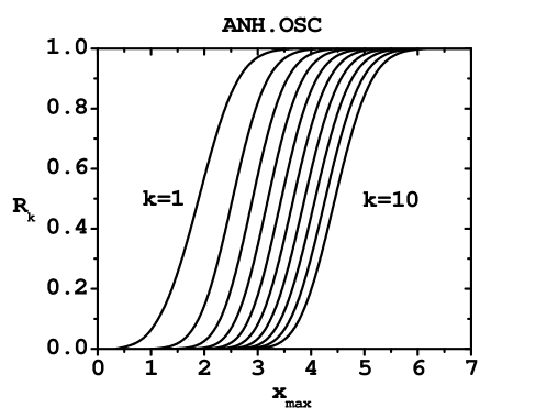
By using this method, we have calculated the first ten coefficients for $\omega=1$ and values of $x_{max}$ between $0.5$ and 7. In order to allow a comparison among the different orders, we define the ratios

$$R_{k}(\sqrt{\omega}x_{max})\equiv E_{0}^{(k)}(\sqrt{\omega}x_{max})/E_{0}^{(k)}(\infty)\ ,$$ (12)

which all tend to 1 in the $x_{max}\rightarrow\infty$ limit and to 0 in the $x_{max}\rightarrow 0$ limit. The numerical values of these ratios are shown in Fig. 1. A striking feature is that the curves for the various orders have approximately the same shape and that we could approximately superpose them by appropriate horizontal translations. Before studying these curves in the large and small $x_{max}$ limits, we will discuss numerical estimates for the radius of convergence of the modified series, that can be extracted from this data.

Figure 1: The numerical values of $R_{k}(x_{\max})$ for $k=1,\dots 10$ and $\omega=1$.

3 Numerical evidence for a finite radius of convergence

If we calculate the integral of a function defined by a series which is uniformly convergent over the range of integration, it is legitimate to interchange the sum and the integral. On general grounds, one would thus expect that if we calculate the partition function of a properly regularized theory (say on a finite lattice) with a field cut, the perturbative expansion becomes convergent for arbitrary complex values of the coupling. The ground state energy of the anharmonic can be obtained from the logarithm of the partition function and consequently, we would expect that its perturbative expansion will have a finite radius of convergence. This radius will depend on the position of the complex zeroes of the partition function.

Figure 2: ln$|E^{(k)}_{0}(x_{max})|$ versus $k$ for $x_{max}$=0.5, 0.7, …1.3 (from bottom to top); $\omega$ was set to 1.

Figure 3: ln$\lambda_{c}(x_{max})$ versus ln$x_{max}$ for $\omega=1$. The line is $4.22-5.89x$.

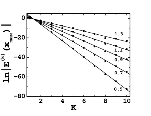
It is sometimes possible to estimate the radius of convergence by considering the empirical asymptotic behavior of the perturbative series. However, with a limited series, transient behavior is often encountered. It is clear from Fig. 1, that if $x_{max}$ is large enough, the beginning of the series looks like its $x_{max}\rightarrow\infty$ limit which grows at a factorial rate. Consequently, in order to attempt to probe the asymptotic behavior, we will only consider $x_{max}$ such that the available coefficients are significantly smaller than their value when $x_{max}$ is infinite. For this reason, we have limited the range of investigation to $x_{max}<1.3$. If we have a finite radius of convergence $\lambda_{c}$, we expect that for $k$ sufficiently large,

$$|E^{(k)}_{0}(\sqrt{\omega}x_{max})|\propto(P(\sqrt{\omega}x_{max}))^{k}$$ (13)

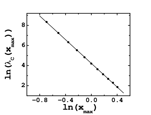
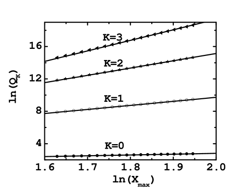
When this is the case, $\lambda_{c}(x_{max},\omega)=\omega^{3}/P(\sqrt{\omega}x_{max})$. In Fig. 3, we have plotted ln$|E^{(k)}_{0}(\sqrt{\omega}x_{max})|$ versus $k$. We see a clear linear behavior and the slope can be interpretated as ln$P(\sqrt{\omega}x_{max})$. We can then study $\lambda_{c}(x_{max},\omega)$ as a function of $x_{max}$. This is done in Fig. 3 where a log-log plot shows a clear linear behavior. The slope is near 5.9 which is close to the value 6 that, we will argue in Sec. 6, should hold in the limit of small $x_{max}$ (see Eq. (40)). We conclude that in this limit, our numerical data suggests

$$\lambda_{c}(x_{max},\omega=1)\simeq 65\times x_{max}^{-6}\ .$$ (14)

4 The large $x_{\max}$ limit

In this section, we first discuss the harmonic energy spectrum with vanishing boundary conditions at $\pm x_{max}$ and then treat the anharmonic interactions with the usual perturbative methods. We work in the limit where $x_{max}$ is large. This means that if we consider the $n$-th energy level, $x_{max}$ should be much larger than the largest zero of $H_{n}(x\sqrt{\omega})$. According to Eq. (6.32.5) of Ref. [12], this imposes the restriction $x_{max}>>\sqrt{2n/\omega}$ for large $n$. When all the zeroes of $H_{n}$ are well within $[-x_{max},x_{max}]$, the new boundary conditions require changes that are exponentially small. It is clear that for any fixed $x_{max}$, this condition will be violated for $n$ sufficiently large.

4.1 The harmonic case

We first need to calculate the energy eigenvalues at $\lambda=0$, $E_{n}^{(0)}(\sqrt{\omega}x_{max}^{2}$), and their corresponding wave functions $\Psi_{n}^{(0)}(x)$. The wave function always depends on $x_{max}$, but this will be kept implicit. We impose the boundary conditions $\Psi_{n}^{(0)^{\prime}}(0)=0$ for $n$ even, $\Psi_{n}^{(0)}(0)=0$ for $n$ odd, and $\Psi^{(0)}(x_{max})=0$ in both cases. We will not pay attention to the overall normalization until the end of the calculation. When $x_{\max}\rightarrow\infty$, we have $E_{n}^{(0)}(\sqrt{\omega}x_{max})\simeq(n+1/2)$ and we will use

$$\epsilon_{n}(\sqrt{\omega}x_{max})\equiv E_{n}^{(0)}(\sqrt{\omega}x_{max})-n-1/2$$ (15)

as our expansion parameter. Again, $\epsilon_{n}$ is a dimensionless quantity that can only depend on $\sqrt{\omega}x_{max}$ and we will often keep this dependence implicit. We write

$$\Psi_{n}^{(0)}(x)\equiv K_{n}^{(0)}(x){\rm e}^{-\omega x^{2}/2}\ .$$ (16)

This corresponds to a choice $G=-\omega x$ in Eqs. (5-6) and consequently

$$-(1/2)K_{n}^{(0)^{\prime\prime}}+\omega xK_{n}^{(0)^{\prime}}-n\omega K_{n}^{(0)}=\epsilon_{n}\omega K_{n}^{(0)}\ .$$ (17)

We then expand

$$K_{n}^{(0)}=K_{n}^{(0)(0)}+\epsilon_{n}K_{n}^{(0)(1)}+\dots$$ (18)

When $x_{max}\rightarrow\infty$, $\epsilon_{n}\rightarrow 0$, and we want to recover the usual harmonic oscillator solution. Consequently, we set $K_{n}^{(0)(0)}(x)=H_{n}(\sqrt{\omega}x)$, the $n$-th Hermite polynomial which is obviously a solution of Eq. (17) at order 0 in $\epsilon_{n}$. At order $\epsilon_{n}$, we have

$$-(1/2)K_{n}^{(0)(1)^{\prime\prime}}+\omega xK_{n}^{(0)(1)^{\prime}}-n\omega K_{n}^{(0)(1)}=\omega H_{n}(\sqrt{\omega}x),$$ (19)

with the boundary conditions

$$K_{n}^{(0)(1)}(0)=K_{n}^{(0)(1)^{\prime}}(0)=0\ .$$ (20)

Remarkably, this inhomogeneous equation can be integrated exactly in two steps. First, we set

$$K_{n}^{(0)(1)}(x)=H_{n}(\sqrt{\omega}x)G_{n}(x)\ .$$ (21)

This removes the explicitly $n$-dependent term and the equation depend only on $G^{\prime}$:

$$-(1/2)H_{n}(\sqrt{\omega}x)G_{n}^{{}^{\prime\prime}}+\left[\omega xH_{n}(\sqrt{\omega}x)-H_{n}^{\prime}(\sqrt{\omega}x)\sqrt{\omega}\right]G_{n}^{{}^{\prime}}=\omega H_{n}(\sqrt{\omega}x),$$ (22)

We then write $G^{\prime}(x)=N(x){\rm e}^{\omega x^{2}}$ which removes the term linear in $x$ and allows us to write the l. h. s. as a total derivative. The solution is then

$$G_{n}(x)=-2\omega\int_{0}^{x}dy(H_{n}(\sqrt{\omega}y))^{-2}{\rm e}^{\omega y^{2}}\int_{0}^{y}dz{\rm e}^{-\omega z^{2}}(H_{n}(\sqrt{\omega}z))^{2}\ ,$$ (23)

One can check that the lower bounds of integration imply the boundary conditions of Eq. (20). This is obvious when $n$ is even. When $n$ is odd, the $z$ integral is of order $y^{3}$ when $y\rightarrow 0$ which overcompensates the $y^{-2}$ of the other factors. Note that $G_{n}(x)$ is independent of $x_{max}$. The integrand of the $y$-integral has a double pole at the zeroes of $H_{n}$, however it has no single pole. This can be seen by plugging a Laurent expansion of $G^{\prime}$ with poles of order 1 and 2 about a zero of $H_{n}$, and using the relation between the first and the second derivative of $H_{n}$ at this zero provided by the defining equation for Hermite polynomials. This forces the coefficient of the simple pole to be zero. Consequently, when we express $G$ as the integral of $G^{\prime}$, we can go around the double pole either above or below the real line and obtain the same result. In other words, we can regularize the $y$-integral by replacing $(H_{n}(\sqrt{\omega}y))^{-2}$ by $(H_{n}(\sqrt{\omega}y)\pm i\epsilon)^{-2}$. From these considerations, we see that $G(x)$ develops a simple pole when $x$ approaches a zero of $H_{n}$, which compensate the simple zero of $H_{n}$. Due to the absence of single pole in $G^{\prime}$, there is no logarithmic singularity in $G$.

$\epsilon_{n}$ can be calculated by imposing the condition that the wave function vanishes at $x_{max}$. This translates into the simple equation:

$$\epsilon_{n}(\sqrt{\omega}x_{max})=-1/G_{n}(x_{max})\ .$$ (24)

As $\epsilon_{n}$ increases, the non-trivial zeroes of the wavefunction move toward the origin. The shift of these zeroes is approximately linear in $\epsilon_{n}$ for large $x_{max}$. For instance, for $n$ =2, the shift of the non-trivial zero $x_{(0)}$ obeys the approximate linear relation $\Delta x_{(0)}\simeq-0.145\epsilon_{2}$.

We now discuss in more detail the case of the ground state ($n=0$). It should be noted that in this case the double integral can be expressed [13] in terms of generalized hypergeometric series

$$G_{0}(x) = -\omega x^{2}\ _{2}F_{2}(1,1;2,3/2;\omega x^{2})$$

$$= -\frac{\sqrt{\pi}}{2}\sum_{k=1}^{\infty}\frac{(\omega x^{2})^{k}}{k\Gamma(k+1/2)}\ .$$

This series defines a function that converges over the entire complex plane. The asymptotic form of $G_{0}(x_{max})$, for $x_{max}$ large, can be worked out by noticing that the integral over $y$ in Eq. (23) comes mostly from the region $y\simeq x_{max}$ and consequently, we can extend the integral over $z$ to infinity with exponentially small errors. The integral over $y$ can then be approximately performed by expanding the argument of the exponential about $x_{max}$. Using Eq. (24), we conclude that asymptotically

$$\epsilon_{0}(\sqrt{\omega}x_{max})\simeq 2\sqrt{\frac{\omega}{\pi}}x_{\max}e^{-\omega x_{\max}^{2}}$$ (26)

This result coincides exactly with the semi-classical estimate given in Ref. [11]. The validity of Eq. (26) can be checked numerically. For instance, for $x_{max}=7$ and $\omega=1$, we get $\epsilon_{0}=4.14\times 10^{-21}$ from Eq. (26) which agrees well with $4.10\times 10^{-21}$ obtained numerically.

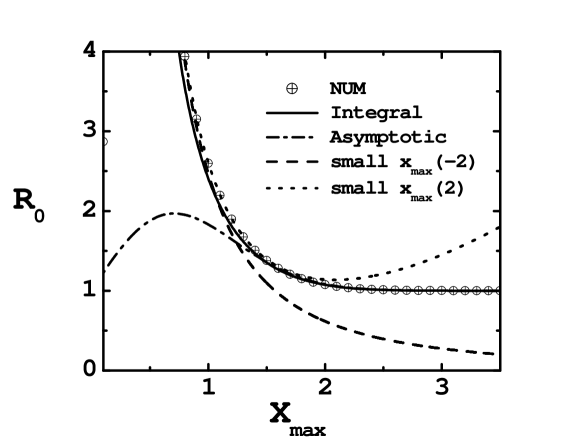
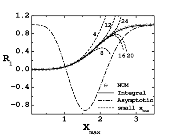
In Fig. 4, we have plotted the asymptotic form Eq. (26) but also the full integral form

$$\epsilon_{0}(\sqrt{\omega}x_{max})=1/(2\omega\int_{0}^{x_{max}}dy{\rm e}^{\omega y^{2}}\int_{0}^{y}dz{\rm e}^{-\omega z^{2}})\ ,$$ (27)

One notices that the integral form stays accurate to much lower values of $x_{max}$, even at very low values of $x_{max}$, where it has no reason to be accurate, it gives a reasonable answer. This observation will be discussed further in Sec. 7.

Figure 4: Numerical values of $R_{0}(x_{max})$ (crossed circles) for $\omega=1$, the integral formula of Eq. (27) (solid line), the asymptotic Eq. (26) (dash-dot line), the leading term ($\propto x_{max}^{-2}$, dash line) of the small $x_{max}$ expansion studied in Sec. 5 and together with the $x_{max}^{2}$ correction (dots). For $x_{max}>1.5$, the integral formula, its asymptotic form and the data are undistinguishable with the eye.

4.2 Anharmonic corrections

Having solved the problem for $\lambda=0$ at first order in $\epsilon_{n}$, we can use the usual methods of perturbation theory. $E_{0}^{(1)}$ can be calculated by taking the average of $x^{4}$ with the corrected ground state wave function constructed above:

$$E^{(1)}_{0}=\omega^{2}N^{-1}\int_{0}^{x_{max}}dx|\Psi_{0}^{(0)}(x)|^{2}x^{4}\ .$$ (28)

with the normalization constant

$$N=\int_{0}^{x_{max}}dx|\Psi_{0}^{(0)}(x)|^{2}\ .$$ (29)

Proceeding as for Eq. (26), we obtain in leading order

$$E^{(1)}\simeq(3/4)-\pi^{1/2}\omega^{5/2}x_{max}^{5}{\rm e}^{-\omega x_{max}^{2}}$$ (30)

Note that in this calculation, we have replaced $G_{0}(x)$ in the integral by its asymptotic form ($\propto x^{-1}{\rm e}^{\omega x^{2}}$ see Eqs. (24 -26)). The exponentials exactly cancel inside the integral and we are left with the integration of $x^{4}/x$. This is justified by the fact that most of the contributions come from the large $x$ region. The validity of the Eq. (30) can be checked numerically. For instance, for $x_{max}=7$ and $\omega=1$, Eq. (30) gives a correction $-4.97\times 10^{-18}$ while numerically we obtain $-5.01\times 10^{-18}$.

The good accuracy of Eq. (30) is shown in Fig. 5. In this figure, we also show the full integral formula of Eq. (28), where the integral was done numerically using the square of the order $\epsilon$ approximation for the ground state wave function, without discarding order $\epsilon^{2}$ terms in the square. Again the integral formula stays valid at unexpectedly low values of $x_{max}$. This will be explained in Sec. 7.

Figure 5: Numerical values of $R_{1}(x_{max})$ (crossed circles) for $\omega=1$, the integral formula of Eq. (28) (solid line), the asymptotic Eq. (30) (dash-dot line), the small $x_{max}$ expansion studied in Sec. 5 truncated at order 4, 8, … 24 (dots). Series analysis suggests that the small $x_{max}$ expansion converges for $x_{max}<2.9$.

The derivation of Eq. (30) is quite simple: $\epsilon_{0}$ give a contribution proportional to $x_{max}e^{-\omega x_{\max}^{2}}$ and the $x$-integral gives a factor $x_{max}^{4}$. We conjecture that at leading order, a similar situation is encountered for higher order terms, and that

$$1-R_{k}(\sqrt{\omega}x_{\max})\propto x_{\max}^{4k+1}e^{-\omega x_{\max}^{2}}\ .$$ (31)

For this purpose we have studied numerically the quantity

$$Q_{k}({\sqrt{\omega}x_{max}})\equiv e^{+\omega x_{\max}^{2}}(1-R_{k}(\sqrt{\omega}x_{\max}))\ ,$$ (32)

which according to the conjecture should scale like $x_{max}^{4k+1}$. In Fig. 6, we have set $\omega=1$ and displayed ${\rm ln}(Q_{k}(x_{max})$ versus ${\rm ln}(x_{max})$. The solid lines represent the linear functions $A_{k}+(4k+1){\rm ln}(x_{max})$. The constants $A_{k}$ have been fitted using the last ten data points. Their numerical values are $A_{0}=0.802$ which compares well with the prediction of Eq. (26) ${\rm ln}(4\pi^{-1/2})\simeq 0.814$, and $A_{1}=-0.276$ which compares well with the prediction of Eq. (30) ${\rm ln}(4\pi^{-1/2}/3)\simeq-0.285$. The linear behavior of the higher orders supports the conjecture.

Figure 6: ${\rm ln}(Q_{k}(x_{max}))$ versus ${\rm ln}(x_{max})$ for $\omega=1$. The explanations about the solid lines is given in the text.

5 The small $x_{\max}$ limit

When the field cutoff $x_{\max}\rightarrow 0$, the potential term in the harmonic oscillator is much smaller then the kinetic term, and in first approximation we can use the free particle in a box of length $2x_{\max}$. The energy levels diverge as $x_{max}^{-2}$ and it is convenient to introduce the following rescalings

$$\tilde{H}=x_{max}^{2}H$$

$$\tilde{x}=x/x_{max}$$

$$\tilde{\omega}=\omega x_{max}^{2}$$

$$\tilde{\lambda}=\lambda x_{max}^{6}$$

We then obtain a new hamiltonian

$$\tilde{H}=-\frac{1}{2}(\frac{d}{d\tilde{x}})^{2}+\tilde{V}\ ,$$ (33)

with

$$\tilde{V}(\tilde{x})=\left\{\begin{array}[]{ccc}\frac{1}{2}\ \tilde{\omega}^{2}\tilde{x}^{2}+\tilde{\lambda}\tilde{x}^{4}&{\rm if}&|\tilde{x}|<1\\ \infty&{\rm if}&|\tilde{x}|\geq 1\end{array}\right.$$ (34)

With these rescalings, $x_{max}$ has disappeared from the problem and we can now expand $\tilde{E}$ as a double series in $\tilde{\lambda}$ and $\tilde{\omega}$. This can be done using the usual methods of perturbation theory since we can solve the problem exactly when $\tilde{\lambda}=\tilde{\omega}=0$. The perturbative series becomes

$$\tilde{E}_{n}=\sum_{k=0,l=0}^{\infty}E_{n}^{(k,l)}\tilde{\lambda}^{k}\tilde{\omega}^{2l}\ ,$$ (35)

with dimensionless coefficients $E_{n}^{(k,l)}$. Scaling back to the original problem, we obtain

$$E_{n}=\sum_{k=0,l=0}^{\infty}E_{n}^{(k,l)}\lambda^{k}\omega^{2l}x_{max}^{6k+4l-2}$$ (36)

Comparing with Eq. (9), we conclude that with this expansion

$$E_{n}^{(k)}(\omega x_{max}^{2})=\sum_{l=0}^{\infty}E_{n}^{(k,l)}\times(\omega x_{max}^{2})^{2l+3k-1}\ .$$ (37)

Obviously, this implies that the asymptotic behavior when $x_{max}\rightarrow 0$, for the ratios displayed in Fig. 1, is

$$R_{k}(\sqrt{\omega}x_{max})\propto x_{max}^{6k-2}$$ (38)

We checked numerically that this asymptotic behavior is correct. Using the data of Fig. 1, one can indeed determine the constant of proportionality $E_{0}^{(l,0)}$ calculated independently below with more than two significant digits.

For the ground state,

$$E_{0}^{(0,0)} = \frac{\pi^{2}}{8}$$

$$E_{0}^{(1,0)} = \frac{1}{5}-\frac{4}{{\pi}^{2}}+\frac{24}{{\pi}^{4}}$$

$$E_{0}^{(0,1)} = \frac{1}{6}-\frac{1}{\pi^{2}}$$ (39)

Higher orders require infinite sums. In practice, since we see from Eq. (34) that the calculations can be performed with $x_{max}=1$, it is easier to proceed numerically as in Sec. 2 but with a double series. The numerical results are given in Table 1 and displayed in Fig. 7.

Table 1: The coefficients $E_{0}^{(k,l)}$.

k \ l	0	1	2	3
0	$1.234\hbox{\phantom{-}}\hbox{\phantom{-}}\hbox{\phantom{-}}$	$\hbox{\phantom{-}}6.535\times 10^{-2}$	$-5.923\times 10^{-4}$	$\hbox{\phantom{-}}6.097\times 10^{-6}$
1	$\hbox{\phantom{-}}4.110\times 10^{-2}$	$-1.169\times 10^{-3}$	$\hbox{\phantom{-}}2.150\times 10^{-5}$	$-2.443\times 10^{-7}$
2	$-6.110\times 10^{-4}$	$\hbox{\phantom{-}}2.555\times 10^{-5}$	$-5.079\times 10^{-7}$	$\hbox{\phantom{-}}3.575\times 10^{-9}$
3	$\hbox{\phantom{-}}1.020\times 10^{-5}$	$-4.571\times 10^{-7}$	$\hbox{\phantom{-}}6.983\times 10^{-9}$	$\hbox{\phantom{-}}9.506\times 10^{-11}$
4	$-1.517\times 10^{-7}$	$\hbox{\phantom{-}}5.804\times 10^{-9}$	$\hbox{\phantom{-}}2.492\times 10^{-11}$	$-7.641\times 10^{-12}$

Figure 7: $ln(|E^{(k,l)}|)$ versus $l$, the order of expansion in $\omega^{2}$, for $k=0,\ 1,\dots\ 5$. The lines represent linear fits for a given $k$.

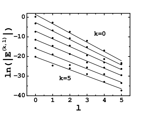
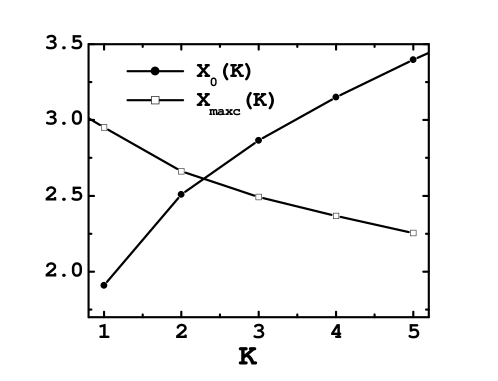
The approximately linear behavior of $ln(|E_{0}^{(k,l)}|)$ in $l$ at fixed $k$ shown in Fig. 7 suggests that the power series in $\omega^{2}x_{max}^{4}$, for the coefficients of $(\lambda/\omega^{3})^{k}$ have a finite radius of convergence (see Eq. (37)). As the slope vary from -4.7 for $k=0$ to -3.3 for $k=5$, we expect that the series converge for $|x_{max}\sqrt{\omega}|<{\rm e}^{4.7/4}\simeq 3.3$ for $k=0$ to ${\rm e}^{3.3/4}\simeq 2.3$ for $k=5$. Fig. 8 shows a steady decrease of the radius of convergence when $k$ increases. At the same time, the value of $x_{max}$ where the transition between the small and large cutoff limit occurs, denoted $x_{0}(k)$ increases with $k$. This quantity is defined more precisely in Sec. 7. Consequently, it seems clear that as the order increases, a gap opens between the range of validity of the small $x_{max}$ expansion and the crossover region.

Figure 8: Estimated values of $x_{max\ c}(k)$ for which we reach the radius of convergence for $\omega=1$ (empty boxes) and values of $x_{0}(k)$ (black circles) where the crossover occurs as defined in Sec. 7, for $k=1,\dots 5$.

6 Rigorous lower bounds ont radius of convergence

In Secs. 3 and 5, we have discussed the radius of convergence of series from a numerical point of view. We now return to this question with more analytical considerations. First of all, it is possible to get an order magnitude estimate for the radius of convergence by using a simple argument. If we look at a typical term of the perturbative series at order $\lambda^{k}$, it is the product of $k$ matrix elements for the perturbation potential $x^{4}$ divided by $k-1$ differences of energy level. The matrix elements of $x^{4}$ are bounded in magnitude by $x_{max}^{4}$. The differences of energy depend on $x_{max}$. If $x_{max}$ is very small, in other words if $x_{max}^{2}\omega^{2}<<\omega$ in units where the mechanical mass and $\hbar$ are set to 1, the harmonic term is a perturbation and the energy differences are proportional to $x_{max}^{-2}$. For instance, the difference between the ground state and the first excited state will be approximately $3\pi^{2}/(8x_{max}^{2})$. In the opposite limit of large $x_{max}$, the level are approximately equidistant with a separation $\omega$. From this we expect that the perturbative series converges for $|\lambda|<\lambda_{c}(x_{max},\omega)$ with

$$\lambda_{c}(x_{max},\omega)\propto\left\{\begin{array}[]{ll}x_{max}^{-6}&{\rm if}\ x_{max}<<\omega^{-1/2}\\ \omega x_{max}^{-4}&{\rm if}\ x_{max}>>\omega^{-1/2}\end{array}\right.$$ (40)

This argument does not take into account aspects such as the number of terms present or their signs, however, a rigorous lower bound on the radius of convergence can be obtained by simply using one half of the difference between the ground state and the first excited state of the unperturbed system in the above argument. This is formulated precisely in Theorem XII.11 in Ref. [14] and proved in Ref. [15]. The final result in our case is

$$\lambda_{c}(x_{max},\omega)>(1/2)(E_{1}^{(0)}-E_{0}^{(0)})/x_{max}^{4}$$ (41)

Note that Theorem XII.11 is more than what we need here because the perturbation is a bounded operator and we do not need to compare its norm with the norm of $H_{0}$.

In the case $\omega=0$, dimensional analysis dictates $\lambda_{c}(x_{max},\omega=0)=Cx_{max}^{-6}$ for some positive $C$, and Eq. (41) implies

$$\lambda_{c}(x_{max},\omega=0)>(3\pi^{2}/16)\times x_{max}^{-6}$$ (42)

This bound can be compared with numerical estimates obtained from the series with coefficients $E_{0}^{(k,0)}$ defined in Sec. 5 and which only requires one calculation with $x_{max}=1$ instead of the two step procedure of Sec. 3. Using the coefficients for $k=5,\dots 10$, we obtain

$$\lambda_{c}(x_{max},\omega=0)\simeq 53\times x_{max}^{-6}\ ,$$ (43)

which is quite close to result obtained with $\omega=1$ at low $x_{max}$ in Sec. 5. The rigorous bound on $C$, $3\pi^{2}/16\simeq 1.85$ is about 30 times smaller than the empirical value 53. In summary, the lower bound is compatible with our numerical estimate, but is not sharp.

The same argument can be applied for the calculation of $E_{0}^{(0)}$ as a power series in $(1/2)\omega^{2}$ for the perturbation $(1/2)\omega^{2}x^{2}$. It can be tested by studying the coefficients $E^{(0,l)}$ as we did in Sec. 5. The rigorous bound becomes $(1/2)\omega^{2}_{c}>(1/2)(3\pi^{2}/8)/x_{max}^{4}$, which implies

$$\omega_{c}>1.92\times x_{max}^{-2}$$ (44)

From Sec. 5, we have

$$\omega_{c}\simeq(3.3)^{2}\times x_{max}^{-2}\ ,$$ (45)

and again, the lower bound is compatible with the numerical estimate, but is not an accurate estimator of the actual radius of convergence.

7 The crossover region: empirical data collapse

In this section, we discuss the question of the interpolation between the large and small $x_{max}$ approximation. In Sec. 4, we have already observed that by naively using integral formulas derived in the large $x_{max}$ approximation for $E^{(0)}$ and $E^{(1)}$, it was possible to obtain decent approximations at low $x_{max}$. We will first explain how this works and then discuss the higher orders terms.

In the (mathematical) limit of very small $x_{max}$, Eq. (23) implies that $G_{0}(x)\simeq-\omega x^{2}$. Consequently, in this limit, where we do not expect the approximation to be accurate, the correction becomes dominant and we have

$$E^{(0)}_{0}(\sqrt{\omega}x_{max})\simeq 1/(\omega x_{max}^{2})\ .$$ (46)

Despite the lack of justification for this formula, it is not far from the accurate answer derived in Sec. 5:

$$E^{(0)}_{0}(\sqrt{\omega}x_{max})\simeq\pi^{2}/(8\omega x_{max}^{2})\simeq 1.234/(\omega x_{max}^{2})$$ (47)

Similarly for $E^{(1)}$, we can study Eq. (28) in the mathematical limit of small $x_{max}$. According to Sec. 4, $\Psi^{(0)}_{0}(x)\simeq(1-(x/x_{max})^{2})$ and elementary integration yields

$$E_{0}^{(1)}(\sqrt{\omega}x_{max})\simeq(1/21)\times(\omega x_{max}^{2})^{2}\simeq 0.0476(\times\omega x_{max}^{2})^{2}$$ (48)

Again, this is close to the accurate answer from Eq. (5):

$$E_{0}^{(1)}(\sqrt{\omega}x_{max})\simeq 0.0411\times(\omega x_{max}^{2})^{2}$$ (49)

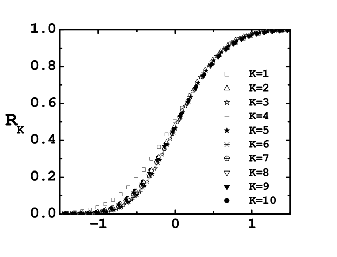
For higher orders, we know from Fig. 8 that the small $x_{max}$ approximation is not convergent in the crossover region. However, the shape similarities observed in Fig. 1 suggest to parametrize $R_{k}$ in terms of a single function $U$, that can be shifted by a $k$-dependent quantity that we denote $x_{0}(k)$. We have chosen $x_{0}(k)$ as the value of $x_{max}$ for which the second derivative of $R_{k}$ vanishes. The numerical values are shown in Table 2 and Fig. 8.

Table 2: $x_{0}(k)$ for $k=1\dots 10$.

• 	$x_{0}(k)$
  1	1.908
  2	2.509
  3	2.868
  4	3.152
  5	3.398
  6	3.626
  7	3.839
  8	4.042
  9	4.235
  10	4.421

Empirically, it can be fitted quite well with

$$x_{0}(k)\simeq 0.87+1.13\sqrt{k}\ .$$ (50)

In Fig. 9, we show that the possibility of having

$$R_{k}(x_{max})\simeq U(x_{max}-x_{0}(k))\ ,$$ (51)

is reasonably well satisfied for $k\geq 2$. In other words, with suitable translations, the $R_{k}$ approximately “collapse”.

Figure 9: $R_{k}(x_{+}x_{0}(k))$ for $k=1,\dots 10$.

8 Conclusions

We have shown that the calculation of the perturbative series for the anharmonic oscillator with a field cutoff $x_{max}$ can be performed reliably using numerical methods, and approximate analytical methods in the limit of small and large $x_{max}$. For the coefficients of order 0 and 1 in $\lambda$, the integral formulas derived in the large $x_{max}$ limit, produce the correct leading power dependence with coefficients close to the correct ones, in the opposite limit (small $x_{max}$) where they are not expected to be accurate. For higher orders, it is possible to approximately collapse the crossover region of the various order by an appropriate translation in $x_{max}$. The collapse is not perfect and it is necessary to resolve more accurately the details of Fig. 9 in order to obtain accurate formulas for the $R_{k}$.

We expect that it is possible to extend the small and large cutoff techniques in the case of higher dimensional field theory, however the only numerical method that can we envision for the crossover region is the Monte Carlo method [16]. In view of this, it is essential to reach a proper understanding of the interpolation.

References

- [1] J. C. LeGuillou and J. Zinn-Justin, Large-Order Behavior of Perturbation Theory (North Holland, Amsterdam, 1990).
- [2] S. Pernice and G. Oleaga, Phys. Rev. D 57, 1144 (1998).
- [3] Y. Meurice, Phys. Rev. Lett. 88, 141601 (2002a), hep-th/0103134.
- [4] C. M. Bender and S. Boettcher, Phys. Rev. Lett. 80, 5243 (1998).
- [5] L. Li and Y. Meurice, Phys. Rev. D 71, 016008 (2005a), hep-lat/0410029.
- [6] B. Kessler, L. Li, and Y. Meurice, Phys. Rev. D69, 045014 (2004), hep-th/0309022.
- [7] L. Li and Y. Meurice, Phys. Rev. D71, 054509 (2005b), hep-lat/0501023.
- [8] I. R. C. Buckley, A. Duncan, and H. F. Jones, Phys. Rev. D47, 2554 (1993).
- [9] A. Duncan and H. F. Jones, Phys. Rev. D47, 2560 (1993).
- [10] C. Bender and T. T. Wu, Phys. Rev. 184, 1231 (1969).
- [11] Y. Meurice, J. Phys. A35, 8831 (2002b), quant-ph/0202047.
- [12] G. Szego, Orthogonal Polynomials (American Mathematical Society, Providence, 1939).
- [13] J. Cook, private communication.
- [14] M. Reed and B. Simon, Methods of Modern Mathematical Physics: IV Analysis of Operators (Academic Press, San Diego, 1978).
- [15] T. Kato, Perturbation Theory for Linear Operators (Springer Verlag, New York, 1966).
- [16] L. Li and Y. Meurice, Nucl. Phys. Proc. Suppl. 129, 883 (2004), hep-lat/0309066.