Abstract

We go on with the definition of the theory of the non–Abelian two–tensor fields and find the gauge transformation rules and curvature tensor for them. To define the theory we use the surface exponent proposed in hep–th/0503234. We derive the differential equation for the exponent and make an attempt to give a matrix model formulation for it. We discuss application of our constructions to the Yang–Baxter equation for integrable models and to the String Field Theory.

1 Introduction

It is well known that the standard theory of fiber bundles is designed to deal with the situations when one has ambiguously defined functions — sections of fiber bundles over a space $X$. In the modern language this means that, knowing the value of a section of a fiber bundle at a point $x$, we can find its value at any other point $y$. But the result will depend on the path taken from $x$ to $y$ and from the choice of the one–form connection on the bundle. The path ordered exponent of the connection gives the map between the fibers $V_{x}$ and $V_{y}$ over the points $x$ and $y$.

This construction assumes that the one–form connection is unambiguously defined up to the gauge transformations — rotations in the fibers. But what if the one–form connection was ambiguous?( The simplest example of such a situation, which we know, is the Wu–Yang monopole.) To describe the situation with the ambiguous one–form connections one has to have a “connection” for the connections — the one to be ordered over the surface inside $X$. The latter orderings give 2D holonomies which describe maps between the sequences of fibers over different curves, along which the original one–form was ordered. One can consult e.g. [1], [2] on the mathematics behind such a construction.

One badly needs a local field theory description of the 2D holonomies in terms of two–tensor fields. In [3] and here we propose such a theory. To get it one has to organize a triangulation–independent area–ordering of two–tensor gauge field carrying color indices. The triangulation–independence is very crucial for the consistency of the theory. It means the following fact. To construct the area–ordering we should approximate the Riemann surfaces by their triangulated versions. For the discretized case the area ordering is obtained as follows. We glue the exponents of the two–tensor field over the whole simplicial surface by putting them at different simplices (triangles), which are sitting at different points inside the base space $X$. Now it is easy to see that the two–tensor connection should carry three color indices along with two spacial ones [3]: $B_{\mu\nu}^{ijk}$, $\mu,\nu=1,\dots,{\rm dim}X$ and $i,j,k=1,\dots,{\rm dim}V$. This is due to the three wedges of each 2D simplex. In [3] we have found a way to exponentiate cubic matrices, which we refer to as the surface exponent. With such an exponent we can take the continuum limit from the simplicial surfaces to the smooth ones. It is important that with the use of the surface exponent the result for the limit will not depend on the way it is taken! This is what we refer to as triangulation–independence.

The organization of the paper is as follows. In the next section we briefly review the paper [3] and concisely formulate its statements. In the section 3 we find the differential equation for the surface exponent and define a new way of the exponentiation of the quadratic matrices. We establish the relation between such an exponent of the quadratic matrices and the surface exponent for the cubic ones. At the end of the section 3 we discuss a possible matrix integral formulation of the surface exponent. In the section 4 we derive the gauge transformation rules and curvature for the two–tensor gauge fields. As well in that section we discuss the meaning of the theory of the non–Abelian tensor fields. In the section 5 we establish links between the latter theory and the lattice integrable models and String Field Theory. We conclude with summary in the section 6.

2 Exponentiation of cubic matrices and the area–ordering

2.1 The surface exponent

In the paper [3] we have defined the surface exponent of a cubic matrix $\hat{B}=||B_{ijk}||$, $i,j,k=1,...,N$ as follows:

$${\rm Tr}\,\left(E^{\hat{B}}_{g,I,\kappa}\right)\equiv\lim_{M\to\infty}\prod_{{\rm graph},g}^{M}\left(\hat{I}+\frac{\hat{B}}{M}\right),$$ (1)

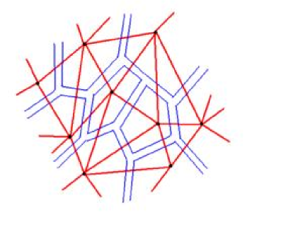
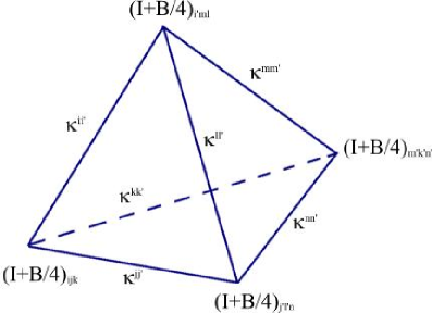
where the limit is taken over a sequence of closed (because on the LHS we take Tr — no any free indices), connected three–valent graphs with $M$ vertices. At a fixed $M$ the product on the RHS of eq.(1)  is taken over an $M$–vertex three–valent graph: At each vertex of the graph we put matrix $I_{ijk}+B_{ijk}/M$ and we glue the indices of these matrices with the use of a bilinear form $\kappa^{ij}$ (as it is shown in the fig. 2). It seem that to take the limit $M\to\infty$ we have to choose a sequence of graphs. But in [3] we have proved that the limit (1) does NOT depend on the choice of the sequence of graphs under the following conditions:

Figure 1: The duality relation between graphs. The three–valent graph is shown here by the fat stripes. The relation between the dual graphs is as follows. We place the vertices of the dual graph at the centers of the faces of the original one and join the vertices via the wedges of the dual graph passing through the wedges of the original one. Thus, the dual graph to a fat three–valent one is the triangulation graph — the graph whose faces are triangles. In this note we are actually using fat three–valent graphs and are frequently changing between three–valent and triangulation graphs.

Figure 2: The example of the product of the matrix $(\hat{I}+\hat{B}/4)$ over the pyramid, i.e. when $M=4$.

• One should consider fat three–valent graphs so that it is obvious on which minimal genus Riemann surface this graph can be mapped. The genus $g$ of the graphs in the sequence should be fixed: I.e. at every $M$ the same topology graphs should be taken.

• The matrices $\hat{I}$ and $\hat{\kappa}$ should obey the following conditions:

  $$I_{ijk}=I_{kij}=I_{jki}-{\rm cyclic\,\,symmetry},$$

  $$\sum_{j,k=1}^{N}{I_{ij}}^{k}\,{I_{lk}}^{j}=\kappa_{il}-{\rm normalization},$$

  $$\sum_{n=1}^{N}I_{inl}\,{I^{n}}_{jk}=\sum_{n=1}^{N}I_{ijn}\,{I^{n}}_{kl}-{\rm fusion}.$$ (2)

  and we higher the indices of $I_{ijk}$ with the use of $\kappa^{ij}$. One can find the graphical representation of the last two equations in the fig. 3.

  

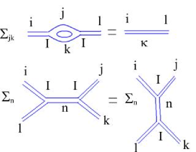
  Figure 3: The two–dimensional conditions which are related to the triangulation independence. These conditions are solved via the use of a semi–simple associative algebra (see e.g. [4], [5], [3]): ${I_{ij}}^{k}=I_{ijl}\,\kappa^{lk}$ are structure constants of this algebra, while $\kappa_{ij}$ is the non–degenerate Killing form. If the algebra is commutative then the matrix $I_{ijk}$ can be mapped (via an orthogonal rotation) to $\delta_{ijk}$ — cubic matrix whose only non–zero elements are units standing on the main diagonal of the cube. In this case the surface exponent can be mapped to the standard one dependent only on the diagonal components of the matrix $\hat{B}$ [3]. The non–trivial case appears when the underlaying semi–simple algebra is non–commutative. The first such case appears when $N=4$ and corresponds to the algebra of $2\times 2$ matrices.

• In the sequence we confine to the graphs of the following kind: As the limit $M\to\infty$ is taken the number of wedges of each face of the graph should be suppressed in comparison with $M$. The geometric meaning of this condition is explained in [3].

In [3] we consider one extra condition. However, this condition is not necessary for the limit (1) to be independent of the choice of the sequence of the graphs. It just simplifies the considerations of [3].

In general at given $N$ there are many solutions to the equations for $\hat{I}$ and $\hat{\kappa}$ and the exponent depends on the choice of $\hat{I}$, $\hat{\kappa}$ and $g$. This explains the subscripts in eq.(1) . The result of the limit is:

$${\rm Tr}\,\left(E^{\hat{B}}_{g,I,\kappa}\right)=\sum_{F=0}^{\infty}\frac{1}{F!}\,B^{j^{(1)}_{1}\,j^{(1)}_{2}\,j^{(1)}_{3}}\dots B^{j^{(F)}_{1}\,j^{(F)}_{2}\,j^{(F)}_{3}}\,I^{g}_{j^{(1)}_{3}\,j^{(1)}_{2}\,j^{(1)}_{1}\left|\dots\right|j^{(F)}_{3}\,j^{(F)}_{2}\,j^{(F)}_{1}},$$ (3)

where we use the same letter $I$ to denote another matrix $I^{g}_{j^{(1)}_{3}\,j^{(1)}_{2}\,j^{(1)}_{1}\left|\dots\right|j^{(F)}_{3}\,j^{(F)}_{2}\,j^{(F)}_{1}}$ with $3F$ indices, which is obtained via multiplication of $I_{ijk}$ over any oriented three–valent graph with $g$ handles, $F$ holes and 3 external wedges at each hole (see fig. 4). At the same time $I^{g}\,(F=0)$ is just a number obtained via the multiplication of $I_{ijk}$ over any closed genus $g$ graph. For example, $I^{0}=\sum_{i,k}\kappa_{i}^{k}\,\kappa_{k}^{i}=\sum_{i}\delta_{i}^{i}=N$. The reason for the division of the indices of $I^{g}_{j^{(1)}_{3}\,j^{(1)}_{2}\,j^{(1)}_{1}\left|\dots\right|j^{(F)}_{3}\,j^{(F)}_{2}\,j^{(F)}_{1}}$ into groups separated by vertical lines is as follows: These matrices are only cyclicly symmetric under the exchange of their indices inside each triple, but are completely symmetric under any exchange of the triples between themselves [3]. All that follows from the topology of the underlaying graphs (see fig. 4) and the condition in fig. 3.

Figure 4: The dual to the three–valent (triangulation) graph defining $I^{g}_{j^{(1)}_{3}\,j^{(1)}_{2}\,j^{(1)}_{1}\left|\dots\right|j^{(F)}_{3}\,j^{(F)}_{2}\,j^{(F)}_{1}}$.

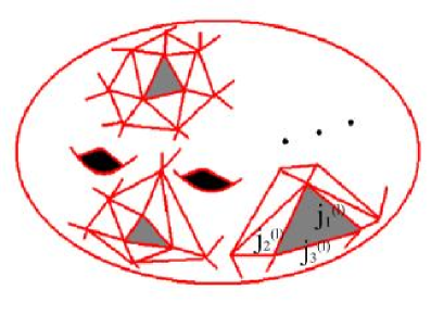
Once we have defined the trace of the surface exponent, we can define the exponent with any number of indices or, better to say, for any two–dimensional topology — for a given number of handles $g$, holes $L$ and distribution of external indices over the holes. To begin with, let us define the exponent for the disc topology and three external wedges at the boundary. To do that in eq.(1)  we have to use open graph with one hole and three wedges at the boundary. The result for the corresponding limit is:

$$\left(E^{\hat{B}}_{I,\kappa}\right)_{m_{1}\,m_{2}\,m_{3}}=\sum_{F=0}^{\infty}\frac{1}{F!}\,B^{j^{(1)}_{1}\,j^{(1)}_{2}\,j^{(1)}_{3}}\dots B^{j^{(F)}_{1}\,j^{(F)}_{2}\,j^{(F)}_{3}}\,I_{\left.m_{1}\,m_{2}\,m_{3}\right|j^{(1)}_{3}\,j^{(1)}_{2}\,j^{(1)}_{1}\left|\dots\right|j^{(F)}_{3}\,j^{(F)}_{2}\,j^{(F)}_{1}}.$$ (4)

The exponent in eq.(4)  is the building block for the construction of a generic surface exponent and for the area–ordering below. In fact, we can glue a two–dimensional surface of any topology with the use of triangles — dual to the three–valent vertices. Now we have to put $\left(E^{\hat{B}}_{I,\kappa}\right)_{m_{1}\,m_{2}\,m_{3}}$ instead of $(I+B/M)_{ijk}$ or $I_{ijk}$ in the vertices. For example, eq.(3)  is obtained via multiplication of eq.(4)  over any genus $g$ closed triangulated Riemann surface: To obtain Tr$E^{\hat{B}}$ we have to take $\hat{B}/J$ in eq.(4) , where $J$ is the total number of triangles out of which the closed surface in question is constructed. This is true due to the main property of the surface exponent which is discussed in the section 3.

2.2 Triangulation–independent area–ordering

With the use of the surface exponent, in [3] we have constructed the triangulation–independent ordering of non–Abelian two–tensor fields over two–dimensional surfaces. Let us repeat that construction here. It is natural to consider, within this context, a triangulated approximation $\tilde{\Sigma}(\tilde{\gamma_{1}},\dots,\tilde{\gamma_{L}})$ of an oriented Riemann surface $\Sigma(\gamma_{1},\dots,\gamma_{L})$ in a target space $X$. This surface has $L$ boundary closed loops $\gamma$’s which are approximated by the closed broken lines $\tilde{\gamma}$’s (see fig. 5). At the end we take the continuum limit and the result does not depend on the way the limit is taken: It does not depend on the choice of the sequence of triangulated surfaces $\tilde{\Sigma}$ which are approaching the smooth surface $\Sigma$ in the limit in question! It is this fact which we refer to as the triangulation independence.

Figure 5: $\tilde{\Sigma}$ is the discretization of $\Sigma$; $\tilde{\gamma}$’s are the discretizations of $\gamma$’s.

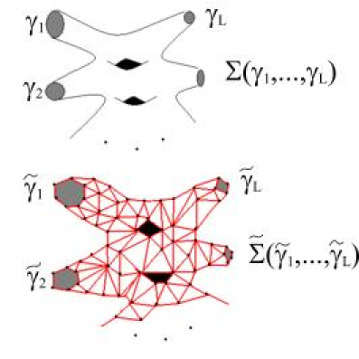
To get the triangulation–independent area–ordering, we have to assign the matrix

$$U_{ijk}(x,\,\Delta\sigma^{\mu\nu})=\left(E_{I,\kappa}^{\hat{B}_{\mu\nu}(x)\,\Delta x^{\mu}\,\Delta x^{\nu}}\right)_{ijk}$$

to each simplex (triangle) sitting at the point $x$ of the image of the triangulated surface in $X$. Here $\Delta\sigma^{\mu\nu}=\Delta x^{\mu}\,\Delta x^{\nu}$ is the oriented area element associated with the triangle in question. The indices $i,j$ and $k$ are assigned to the three wedges of the corresponding triangle. Hence, $\hat{U}:V^{3}\to\mathbb{C}$ for an $N$–dimensional vector space $V$ — the “fiber” of our ”fiber bundle”, while $X$ is the base of the bundle.

The area–ordering is obtained by gluing, via the use of the bi–linear form $\kappa^{ij}:\mathbb{C}\to V^{2}$, the matrices $U_{ijk}$ on each triangle over the whole simplicial surface (see fig. 6):

$$U\left[\tilde{\Sigma}(\tilde{\gamma_{1}},\dots,\tilde{\gamma_{L}})\right]_{j^{(1)}_{1}\dots j^{(1)}_{n_{1}}\left|j^{(2)}_{1}\dots j^{(2)}_{n_{2}}\right|\dots\left|j^{(L)}_{1}\dots j^{(L)}_{n_{L}}\right.}\equiv$$

$$\equiv\sum_{k_{1},k_{2},\dots,k_{w}}U_{j^{(1)}_{1}\,k_{1}\,k_{2}}\left(x_{1}^{\phantom{\frac{1}{2}}},\Delta\sigma_{1}\right)\,{U^{k_{1}\,k_{3}}}_{k_{4}}\left(x_{2}^{\phantom{\frac{1}{2}}},\Delta\sigma_{2}\right)\,{U^{k_{3}}}_{j^{(1)}_{2}\,j^{(1)}_{3}}\left(x_{3}^{\phantom{\frac{1}{2}}},\Delta\sigma_{3}\right)\dots$$ (5)

where $w$ is the total number of internal wedges of the graph; $j^{(l)}$ are the indices corresponding to the wedges of the $l$-th broken line $\tilde{\gamma}_{l}$ and $n_{l}$ is the total number of the wedges of this broken line. We higher (lower) the indices via the use of the aforementioned bilinear form $\kappa^{ij}$ ($\kappa_{ij}\kappa^{jk}=\delta_{i}^{k}$).

Figure 6: This is a fragment of $\tilde{\Sigma}(\tilde{\gamma}_{1},\dots,\tilde{\gamma}_{L})$. On each triangle of this figure there is $U$ matrix with three indices and we sum over the indices assigned to the internal wedges of the graph.

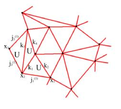
In the continuum limit the discrete indices $1,...,n_{l}$ are converted into the continuum ones $s_{l}\in[0,\,2\pi)$ and we obtain:

$$U\left[\tilde{\Sigma}(\tilde{\gamma_{1}},\dots,\tilde{\gamma_{L}})\right]_{j^{(1)}_{1}\dots j^{(1)}_{n_{1}}\left|j^{(2)}_{1}\dots j^{(2)}_{n_{2}}\right|\dots\left|j^{(L)}_{1}\dots j^{(L)}_{n_{L}}\right.}\longrightarrow U\left[\Sigma^{\phantom{\frac{1}{2}}}(\gamma_{1},\dots,\gamma_{L})\right]_{j^{(1)}(s_{1})\left|j^{(2)}(s_{2})\right|\dots\left|j^{(L)}(s_{L})\right.},$$

$${\rm where}\quad\hat{U}(\Sigma):V^{\infty}(1)\otimes\dots\otimes V^{\infty}(L)\to\mathbb{C}.$$ (6)

Here $j^{(l)}(s_{l})$ is the “color” index assigned to the continuous number of points enumerated by $s_{l}$ — a parametrization of the $l$-th loop $\gamma_{l}$. The expression (6) is not so unfamiliar for the string theoreticians as it could seem from the first sight. In fact, if we substitute $j^{(l)}(s_{l})$ by $x^{(l)}(s_{l})$, then $U\left[\Sigma(\gamma_{1},\dots,\gamma_{L})\right]$ can be considered as a kind of string amplitude whose end–loops $\gamma$’s are mapped by $x(s)$’s. This is the subject of the section 5.

Using the surface exponent (4), we can write the explicit expression for the area–ordered exponent (“$A\,E$”) (5)–(6). For example, for the case of the disc $D$ we obtain:

$$U_{j(s)}(D,\hat{B})=\left(A\,E_{g,I,\kappa}^{{\int\int}_{D}\hat{B}_{\mu\nu}\,dx_{\mu}\,dx_{\nu}}\right)_{j(s)}\equiv\sum_{F=0}^{\infty}\frac{1}{F!}\,I^{g}_{\left.j(s)\right|j^{(1)}_{3}\,j^{(1)}_{2}\,j^{(1)}_{1}\left|\dots\right|j^{(F)}_{3}\,j^{(F)}_{2}\,j^{(F)}_{1}}\,\times$$

$$\times{\int\int}_{D}B_{\mu_{1}\nu_{1}}^{j^{(1)}_{1}\,j^{(1)}_{2}\,j^{(1)}_{3}}dx_{\mu_{1}}\,dx_{\nu_{1}}\dots\int\int_{D}B_{\mu_{F}\nu_{F}}^{j^{(F)}_{1}\,j^{(F)}_{2}\,j^{(F)}_{3}}dx_{\mu_{F}}\,dx_{\nu_{F}}=\left(E_{g,I,\kappa}^{{\int\int}_{D}\hat{B}_{\mu\nu}\,dx_{\mu}\,dx_{\nu}}\right)_{j(s)},$$ (7)

where $s$ is the parametrization of the boundary and $j(s)$ is the index function at the boundary $\partial D$. The last equality holds because of the symmetry properties of the matrices $I_{\left.j(s)\right|j^{(1)}_{3}\,j^{(1)}_{2}\,j^{(1)}_{1}\left|\dots\right|j^{(F)}_{3}\,j^{(F)}_{2}\,j^{(F)}_{1}}$. These properties are discussed below the eq.(3) . As the result, such an area–ordering is rather trivial because there is no need to order anything. In fact, we can easily interchange the order of integrals over $B$ in eq.(7) . This should be the generic property of all “higher dimensional” exponents (for multi-index matrices) due to the triviality of the corresponding homotopy groups.

Let us clarify this important subject. In the one–dimensional ordering for one–form gauge fields the order is important for the following reason: If one throws away a point (insertion of a local observable) from an open curve (along which the ordering is done) it becomes disconnected. Then it is important what is on the left and what is on the right from the point in question. On the other hand, in the case of two–dimensional orderings, throwing away a point is not sufficient to make the surface disconnected. Hence, the order is unimportant. As the result there are no commutators of local fields which describe two–dimensional area–orderings. We come back to this point again at the end of the section 4.

However, the commutative nature of the area–ordering does not mean that we have obtained something trivial! In fact, if we consider a surface $\Sigma$ with one designated point $x$ and two external wedges at this point the corresponding $U(\Sigma_{x})_{ij}$ (or ${U(\Sigma_{x})_{i}}^{j}=U(\Sigma_{x})_{ik}\,\kappa^{kj}$) gives a nontrivial (non–diagonal matrix) map. All that goes without saying that more complicated matrices ${U(\Sigma_{x,y,\dots})_{ijm\dots}}^{kl\dots}$ give completely non–trivial non–linear maps. Somehow the latter objects intrinsically include interactions because the $B$–field and especially the background $\hat{I}$ give non–linear maps ($\hat{B},\hat{I}:V^{3}\to\mathbb{C}$). As the result $U$’s give non–trivial non–linear maps between the end–loops of the corresponding surfaces.

In any case, to our mind this is a deep fact which is yet to be understood to establish the relation of the subject in question to the String Field Theory and to the standard theory of fiber bundles. Note that in [6] we describe how to construct modified surface “exponent”, which obeys less trivial relations, and we think that the surface exponent can appear in the applications in the latter form.

3 Relevant properties of the exponent

3.1 Differential equation for the exponent

Let us derive the differential equation for the surface exponent. To do that recall that the exponent of a quadratic matrix ${A_{i}}^{j}$ has the following main property (which is at the basis of the probability theory and all evolution phenomena):

$${\left(e^{t_{1}\,\hat{A}}\right)_{i}}^{j}\,{\left(e^{t_{2}\,\hat{A}}\right)_{j}}^{k}={\left(e^{\left(t_{1}+t_{2}\right)\,\hat{A}}\right)_{i}}^{k}$$ (8)

for any two numbers $t_{1}$ and $t_{2}$. This equation defines the exponent unambiguously. In fact, from eq.(8)  one can derive the differential equation for the exponent: Choose $t_{1}=t$ and $t_{2}=dt\ll t$. Then, expanding over $dt$ both sides of eq.(8) , we obtain:

$$\frac{d}{dt}\left(e^{t\hat{A}}\right)_{i}^{j}=A_{i}^{k}\left(e^{t\hat{A}}\right)_{k}^{j}.$$ (9)

The surface exponent can have any number of external indices — not only zero or two like the exponent of a quadratic matrix. As the result it obeys many different identities following from the conditions of the triangulation independence. But all these conditions originate from the basic one:

$${\left(E_{I,\kappa}^{t_{1}\,\hat{B}}\right)_{j_{1}\,j_{2}}}^{k_{1}}\,\left(E_{I,\kappa}^{t_{2}\,\hat{B}}\right)_{j_{3}\,j_{4}k_{1}}=\left(E_{I,\kappa}^{\left(t_{1}+t_{2}\right)\,\hat{B}}\right)_{j_{1}\,j_{2}\,j_{3}\,j_{4}},$$ (10)

which is shown graphically in the fig. 7. This equation, however, does not define unambiguously the surface exponent, because $\hat{I}$ and $\hat{\kappa}$ do not explicitly present in this equation.

Figure 7: The basic condition for the surface exponent shown for the example of the triangulation graphs.

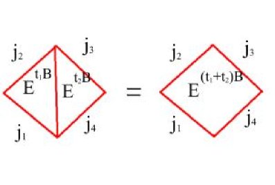
However, if $t_{1}=t$ and $t_{2}=dt\ll t$, we can obtain the following differential equation:

$$\frac{d}{dt}{\left(E_{I,\kappa}^{t\,\hat{B}}\right)_{j_{1}\,j_{2}}}^{k_{1}}\,I_{j_{3}\,j_{4}\,k_{1}}={\left(E_{I,\kappa}^{t\,\hat{B}}\right)_{j_{1}\,j_{2}}}^{k_{1}}\,B_{j_{3}\,j_{4}\,k_{1}},$$ (11)

which fixes the exponent unambiguously for a particular choice of $\hat{I}$ and $\hat{\kappa}$ matrices, because now they are explicitly present in the equation.

Similarly one can write the variational equation for the area–ordered exponent (7):

$$\frac{\delta^{2}}{\delta\sigma_{\mu\nu}^{2}(s)}\left(E_{g,I,\kappa}^{{\int\int}_{D}\hat{B}_{\mu\nu}\,dx_{\mu}\,dx_{\nu}}\right)_{\dots\,j_{s}}\,I^{j_{s}kl}=\left(E_{g,I,\kappa}^{{\int\int}_{D}\hat{B}_{\mu\nu}\,dx_{\mu}\,dx_{\nu}}\right)_{\dots\,j_{s}}\,B^{j_{s}kl}_{\mu\nu}\left[x(s)\right],$$ (12)

where $\delta^{2}/\delta\sigma_{\mu\nu}^{2}(s)$ is the standard variation with respect to the addition of a small area $(\Delta\sigma^{\mu\nu})$ to the disc $D$ and $j_{s}$ means single index $j$ at the point $s$.

3.2 New way to exponentiate quadratic matrices and its relation to the surface exponent

In this subsection we will define non–standard way of exponentiation of quadratic matrices. It is inspired by the surface exponent. In fact, we can put in the vertices of the graphs in eq.(1)  the matrix $I_{ijk}$ rather than $I_{ijk}+B_{ijk}/M$, but glue their indices with the use of $\kappa^{ij}+B^{ij}/W$ rather than just with the use of $\kappa^{ij}$, i.e.:

$${\rm Tr}\,\left(\tilde{E}^{\hat{B}}_{g,I,\kappa}\right)\equiv\lim_{W\to\infty}\prod_{{\rm graph}(g)}^{W}\left(\hat{\kappa}+\frac{\hat{B}}{W}\right),$$ (13)

where under “graph” we assume the same kind of three–valent genus $g$ closed graph as in eq.(1) , which has $W$ wedges. In the light of the above discussion the limit (13) does not depend on the choice of the sequence of graphs. The result for the limit is:

$${\rm Tr}\,\left(\tilde{E}^{\hat{B}}_{g,I,\kappa}\right)=\sum_{F=0}^{\infty}\frac{1}{F!}\,B^{j^{(1)}_{1}\,j^{(1)}_{2}}\dots B^{j^{(F)}_{1}\,j^{(F)}_{2}}\,I^{g}_{j^{(1)}_{1}\,j^{(1)}_{2}\left|\dots\right|j^{(F)}_{1}\,j^{(F)}_{2}},$$ (14)

where $I^{g}_{j^{(1)}_{1}\,j^{(1)}_{2}\left|\dots\right|j^{(F)}_{1}\,j^{(F)}_{2}}$ is the matrix with $2F$ indices obtained via multiplication of $I_{ijk}$ over any oriented graph with $g$ handles, $F$ holes and 2 external wedges at each hole. Similarly we can define exponents with any distribution of indices.

Now we are going to show that this exponent is equivalent to the original one. In fact, it is easy to see that:

$$\lim_{W\to\infty}\prod_{{\rm graph}(g)}^{W}\left(\hat{\kappa}+\frac{\hat{B}}{W}\right)=\lim_{W\to\infty}\prod_{{\rm graph}(g)}^{W}\left(\hat{\kappa}+\frac{\hat{B}}{2\,W}\right)^{2}=\lim_{M\to\infty}\prod_{{\rm graph}(g)}^{M}\left(1+\frac{\hat{B}}{3\,M}\right)^{3}\hat{I},$$ (15)

where $M$ is the number of vertices of the same graph. (Note that $2\,W=3\,M$ for the three–valent graphs.) In the last expression of eq.(15)  we put in the vertices the following matrix:

$$\left(1+\frac{\hat{B}}{3\,M}\right)^{3}\hat{I}\equiv\left|\left|\left(1+\frac{B}{3\,M}\right)^{i^{\prime}}_{i}\left(1+\frac{B}{3\,M}\right)^{j^{\prime}}_{j}\left(1+\frac{B}{3\,M}\right)^{k^{\prime}}_{k}I_{i^{\prime}j^{\prime}k^{\prime}}\right|\right|=$$

$$=\left|\left|I_{ijk}+\frac{B^{i^{\prime}}_{i}}{3\,M}\,I_{i^{\prime}jk}+\frac{B^{j^{\prime}}_{j}}{3\,M}\,I_{ij^{\prime}k}+\frac{B^{k^{\prime}}_{k}}{3\,M}\,I_{ijk^{\prime}}+{\cal O}\left(\frac{1}{M^{2}}\right)\right|\right|.$$ (16)

We higher the indices in this expression with the use of $\kappa^{ij}$ and use in eq.(15)  and eq.(16)  the fact that $\kappa_{ij}\,\kappa^{jk}=\delta_{i}^{k}$. In the limit $M\to\infty$ the terms ${\cal O}(1/M^{2})$ in the eq.(16)  do not survive and we obtain the relation between the cubic and quadratic matrices:

$$\tilde{B}_{ijk}=\frac{B^{i^{\prime}}_{i}}{3}\,I_{i^{\prime}jk}+\frac{B^{j^{\prime}}_{j}}{3}\,I_{ij^{\prime}k}+\frac{B^{k^{\prime}}_{k}}{3}\,I_{ijk^{\prime}}$$ (17)

for which the following equality holds:

$$\tilde{E}^{\hat{B}}_{g,I,\kappa}=E^{\hat{\tilde{B}}}_{g,I,\kappa}.$$ (18)

Thus, basically we have the unique “two–dimensional” exponent. It is worth pointing out now that all the relevant properties of the surface exponent are due to the fact that it is the background $I_{ijk}$ who carries three color indices rather than the matrix $B_{ijk}$ under the exponent. In any case, we are going to use the new way of exponentiation of the quadratic matrices in the section 4.

3.3 Towards Matrix model representation for the exponent

In this subsection we discuss our attempts to represent the surface exponent via the use of a matrix integral. In fact, the mentioned above matrices $I^{g}_{j^{(1)}_{3}\,j^{(1)}_{2}\,j^{(1)}_{1}\left|\dots\right|j^{(F)}_{3}\,j^{(F)}_{2}\,j^{(F)}_{1}}$ are 2D topological invariants in the sense discussed say in [5]. This is true due to the conditions (2) imposed on $\hat{I}$ and $\hat{\kappa}$: The matrix $I^{g}_{j^{(1)}_{3}\,j^{(1)}_{2}\,j^{(1)}_{1}\left|\dots\right|j^{(F)}_{3}\,j^{(F)}_{2}\,j^{(F)}_{1}}$ depends only on the topology of the discretized Riemann surface, but does not depend on its concrete triangulation. We would like to write an explicit representation for this matrix through the correlation function in a 2D topological theory.

To do that let us consider the matrix integral, which is a generalization of the integral considered in [7]:

$$Z(K,\,N,\,\kappa,\,I)=\int\prod_{i=1}^{N}d\hat{\Phi}^{i}\,\exp\left\{-K\,{\rm Tr}\left[\hat{\Phi}^{i}\,\hat{\Lambda}\,\hat{\Phi}^{j}\,\kappa_{ij}+\frac{\rm i}{3}\,I_{ijk}\,\hat{\Phi}^{i}\,\hat{\Phi}^{j}\,\hat{\Phi}^{k}\right]\right\},$$ (19)

where from now on we put $\hat{\Lambda}=1$. The integral is taken over the unitary matrices $\hat{\Phi}_{i}=||\Phi_{i}^{ab}||$, where $i=1,...,N$ and $a=1,...,K$. Taylor expanding this integral over the powers of $I_{ijk}$ and using the decoupling of correlations for the Gaussian integral, usually referred to as Wick’s theorem, we obtain the Feynman diagram expressions for the contributions to the integral. Then, it is easy to see that:

$$\left.\frac{\partial^{\chi(g)}}{\partial K^{\chi(g)}}Z(K,\,N,\,\kappa,\,I)\right|_{K=0}\propto I^{g},\quad g\geq 1,$$ (20)

because by taking this derivative we extract the genus $g$, three–valent, closed graph (Feynman diagram), where in the vertices the matrix $I_{ijk}$ is standing, while in the wedges one puts the “propagator” $\kappa^{ij}$ ($\kappa^{ij}\,\kappa_{jk}=\delta^{i}_{k}$). Note that the integral (19) is convergent and explicitly calculable:

$$\log Z(K,\,N,\,\kappa,\,I)=\sum_{g=0}^{\infty}C_{g}\,K^{\chi(g)}\,I^{g},$$ (21)

where $C_{g}$ are some combinatorial coefficients counting the numbers (with alternating signs) of three–valent connected graphs at the given $g$.

It seems that by considering the $g$ handle contribution to the correlation function:

$$\int\prod_{i=1}^{N}d\hat{\Phi}^{i}\,:\hat{\Phi}_{j_{3}^{(1)}}\,\hat{\Phi}_{j_{2}^{(1)}}\,\hat{\Phi}_{j_{1}^{(1)}}:\dots:\hat{\Phi}_{j_{3}^{(F)}}\,\hat{\Phi}_{j_{2}^{(F)}}\,\hat{\Phi}_{j_{1}^{(F)}}:\,\exp\left\{-K\,{\rm Tr}\left[\hat{\Phi}^{i}\,\hat{\Phi}^{j}\,\kappa_{ij}+\frac{\rm i}{3}\,I_{ijk}\,\hat{\Phi}^{i}\,\hat{\Phi}^{j}\,\hat{\Phi}^{k}\right]\right\}$$ (22)

will give us the desired matrix $I^{g}_{j^{(1)}_{3}\,j^{(1)}_{2}\,j^{(1)}_{1}\left|\dots\right|j^{(F)}_{3}\,j^{(F)}_{2}\,j^{(F)}_{1}}$ if we do not Wick contract the $\hat{\Phi}$’s inside the “normal ordering” — $:\Phi\,\Phi\,\Phi:$. In fact, this correlation function gives a 2D topological invariant in the sense of [5]. However this topological invariant does not coincide with $I^{g}_{j^{(1)}_{3}\,j^{(1)}_{2}\,j^{(1)}_{1}\left|\dots\right|j^{(F)}_{3}\,j^{(F)}_{2}\,j^{(F)}_{1}}$ because we can not separate the contact terms from the desired ones: In the result of the calculation of the genus $g$ contribution to the eq.(22)  (if $F=2$), along with the matrix $I^{g}_{\left.j^{(1)}_{3}\,j^{(1)}_{2}\,j^{(1)}_{1}\right|j^{(2)}_{3}\,j^{(2)}_{2}\,j^{(2)}_{1}}$ the following kind of contribution appears: $I^{g}_{j^{(1)}_{3}\,j^{(1)}_{2}\,j^{(2)}_{2}\,j^{(2)}_{1}}\cdot\kappa_{j^{(1)}_{1}\,j^{(2)}_{3}}$ — one of the contact terms.

At this stage we do not know how to separate this two kinds of contributions to the correlation functions (22). However, we would like to find a way to do that, because it will establish a closer relation of our considerations to the subject of the String Field Theory.

4 Theory of non–Abelian two–tensor fields

In this section we discuss gauge transformations and curvature for the two–tensor gauge connection. To explain the idea of our argument and to set the notations let us present here the derivation of the gauge transformation and curvature of an ordinary gauge field. Consider a holonomy matrix

$$\hat{U}(x,\,\Delta x)=e^{{\rm i}\,\hat{A}_{\mu}(x)\,\Delta x^{\mu}}$$

for a small $\Delta x$. This matrix transforms, under the rotations in the fibers, as:

$$\hat{\widetilde{U}}(x,\,\Delta x)=\hat{g}^{-1}(x)\,\hat{U}(x,\,\Delta x)\,\hat{g}(x+\Delta x).$$

Then, expanding in powers of $\Delta x$ both sides of this expression, we obtain:

$$\hat{\widetilde{A}}_{\mu}(x)=\hat{g}^{-1}(x)\,\left[\partial_{\mu}+{\rm i}\,\hat{A}_{\mu}(x)\right]\,\hat{g}(x).$$

Which is the gauge transformation for the gauge field.

As well, by considering the holonomy matrix for a small square loop and expanding in powers of its size, we obtain:

$$\hat{U}(x,\Delta x^{\mu})\,\hat{U}(x+\Delta x^{\mu},\Delta x^{\nu})\,\hat{U}^{+}(x+\Delta x^{\nu},\Delta x^{\mu})\,\hat{U}^{+}(x,\Delta x^{\nu})=1+{\rm i}\hat{F}_{\mu\nu}\,\Delta x^{\mu}\,\Delta x^{\nu}+\dots,$$ (23)

where $\hat{F}_{\mu\nu}=\partial_{[\mu}\,\hat{A}_{\nu]}-{\rm i}\,\left[\hat{A}_{\mu},\,\hat{A}_{\nu}\right]$.

Obviously for the two–form gauge connection everything works in a similar way if we substitute the line holonomy for quadratic matrices with the surface holonomy for cubic ones. For example, it seems to be natural to postulate the following transformation for the area–ordered exponent over the disc $D$:

$$\left(E_{I,\kappa}^{{\int\int}_{D}\hat{\widetilde{B}}_{\mu\nu}\,dx_{\mu}\,dx_{\nu}}\right)_{j(s)}=\left(E_{I,\kappa}^{{\int\int}_{D}\hat{B}_{\mu\nu}\,dx_{\mu}\,dx_{\nu}}\right)_{k(s)}\,{\left(e^{{\rm i}\,\oint_{\partial D}ds\,\dot{x}^{\mu}\,\hat{A}_{\mu}}\right)^{k(s)}}_{j(s)},$$ (24)

where $s$ is the parametrization of the boundary and $j(s)$ and $k(s)$ are the index functions at the boundary $\partial D$. Here

$${\left(e^{{\rm i}\,\oint_{\partial D}ds\,\dot{x}^{\mu}\,\hat{A}_{\mu}}\right)^{k(s)}}_{j(s)}=\lim_{|\Delta x|\to 0,L\to\infty}\prod_{a=1}^{L}{\left(e^{{\rm i}\,\hat{A}_{\mu}(x_{a})\Delta x^{\mu}}\right)^{k_{a}}}_{j_{a}}$$ (25)

is a kind of a hedgehog line — “Wilson line” with all free (without contraction) indices of all $\hat{A}$’s at each $s\in[0,2\pi)$. The exponent here is just the standard one for quadratic matrices.

However the $B$–field can not transform in this way. In fact, consider such a transformation for a small square with four external indices (see fig. 8):

Figure 8: Disc topology with four external wedges.

$$\left(E_{I,\kappa}^{\hat{\widetilde{B}}_{\mu\nu}[x]\,\Delta x^{\mu}\,\Delta x^{\nu}}\right)_{k_{1}\,k_{2}\,n}\,{\left(E_{I,\kappa}^{\hat{\widetilde{B}}_{\mu\nu}\left[x\right]\,\Delta x^{\mu}\,\Delta x^{\nu}}\right)^{n}}_{k_{3}\,k_{4}}=\left(E_{I,\kappa}^{\hat{B}_{\mu\nu}[x]\,\Delta x^{\mu}\,\Delta x^{\nu}}\right)_{j_{1}\,j_{2}\,n}\times$$

$$\times{\left(E_{I,\kappa}^{\hat{B}_{\mu\nu}\left[x\right]\,\Delta x^{\mu}\,\Delta x^{\nu}}\right)^{n}}_{j_{3}\,j_{4}}\,{\left(e^{{\rm i}\,\hat{A}_{\mu}\Delta x^{\mu}}\right)^{j_{1}}}_{k_{1}}\,{\left(e^{{\rm i}\,\hat{A}_{\nu}\Delta x^{\nu}}\right)^{j_{2}}}_{k_{2}}\,{\left(\,e^{-{\rm i}\,\hat{A}_{\mu}\Delta x^{\mu}}\right)^{j_{3}}}_{k_{3}}\,{\left(e^{-{\rm i}\,\hat{A}_{\nu}\Delta x^{\nu}}\right)^{j_{4}}}_{k_{4}}.$$ (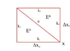26)

Expanding this expression in powers of $\Delta x$, we obtain:

$$2\,I_{k_{1}\,k_{2}\,k_{3}\,k_{4}|m_{3}\,m_{2}\,m_{1}}\,\widetilde{B}^{m_{1}\,m_{2}\,m_{3}}_{\mu\nu}\,\Delta x^{\mu}\,\Delta x^{\nu}=2\,I_{k_{1}\,k_{2}\,k_{3}\,k_{4}|m_{3}\,m_{2}\,m_{1}}\,B^{m_{1}\,m_{2}\,m_{3}}_{\mu\nu}\,\Delta x^{\mu}\,\Delta x^{\nu}+$$

$$+{\rm i}\,I_{j_{1}\,j_{2}\,j_{3}\,j_{4}}\,\left[\left(A_{\mu}\,\Delta x^{\mu}\right)^{j_{1}}_{k_{1}}\,\delta^{j_{2}}_{k_{2}}\,\delta^{j_{3}}_{k_{3}}\,\delta^{j_{4}}_{k_{4}}-\delta^{j_{1}}_{k_{1}}\,\delta^{j_{2}}_{k_{2}}\,\left(A_{\mu}\,\Delta x^{\mu}\right)^{j_{3}}_{k_{3}}\,\delta^{j_{4}}_{k_{4}}\right]+$$

$$+{\rm i}\,I_{j_{1}\,j_{2}\,j_{3}\,j_{4}}\,\left[\delta^{j_{1}}_{k_{1}}\,\left(A_{\nu}\,\Delta x^{\nu}\right)^{j_{2}}_{k_{2}}\,\delta^{j_{3}}_{k_{3}}\,\delta^{j_{4}}_{k_{4}}-\delta^{j_{1}}_{k_{1}}\,\delta^{j_{2}}_{k_{2}}\,\delta^{j_{3}}_{k_{3}}\,\left(A_{\nu}\,\Delta x^{\nu}\right)^{j_{4}}_{k_{4}}\right]+\dots$$ (27)

We do not spell here the higher terms in $A$ because they are not relevant to observe that there is no way to transform the $B$–field to compensate the linear terms in $\Delta x$.

Then we propose that the area–ordered exponent transforms with the use of the surface exponent:

$$\left(E_{I,\kappa}^{{\int\int}_{D}\hat{\widetilde{B}}_{\mu\nu}\,dx_{\mu}\,dx_{\nu}}\right)_{j(s)}=\left(E_{I,\kappa}^{{\int\int}_{D}\hat{B}_{\mu\nu}\,dx_{\mu}\,dx_{\nu}}\right)_{k(s)}\,{\left(\tilde{E}_{I,\kappa}^{{\rm i}\,\oint_{\partial D}ds\,\dot{x}^{\mu}\,\hat{A}_{\mu}}\right)^{k(s)}}_{j(s)},$$ (28)

where we consider it more natural to integrate the quadratic matrix $\hat{A}_{\mu}=||A^{ab}_{\mu}||$ (rather than a cubic one) over the boundary of the disc $\partial D$. Hence in this expression we are using the exponent defined in the subsection 3.2.

Now if we take the disc as in the fig. 8 and expand both sides of the corresponding expression (analogous to eq.(26) ) in powers of $\Delta x$, we observe that all the linear terms (as in eq.(27) ) do cancel out and no other dangerous terms appear. As the result the $B$–field transforms as:

$$\tilde{B}^{ijk}_{\mu\nu}=B^{ijk}_{\mu\nu}+{\rm i}\,\frac{{\partial_{[\mu}A_{\nu]}}^{i}_{l}}{3}\,I^{ljk}+{\rm i}\,\frac{{\partial_{[\mu}A_{\nu]}}^{j}_{l}}{3}\,I^{ilk}+{\rm i}\,\frac{{\partial_{[\mu}A_{\nu]}}^{k}_{l}}{3}\,I^{ijl},$$ (29)

i.e. as a collection of the Abelian stringy $B$–fields for each group of indices $i,j,k$. This is not a surprise for us once we understood the main properties of the surface exponent, which are discussed at the end of the section 2.

Figure 9: Holonomy matrix for cube gives the curvature of the $B$–field.

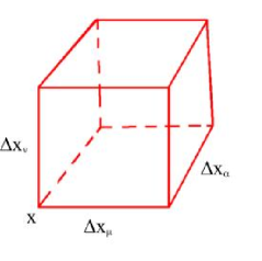
We can calculate as well the curvature of the “non–Abelian” $B$–field. To do that we have to consider a small closed surface having the geometry of the cube (see fig. 9). Then the corresponding holonomy matrix has the following expansion:

$${\rm Tr}\,\left[\hat{U}\left(x,\Delta x^{\mu}\Delta x^{\nu}\right)\hat{U}\left(x+\Delta x^{\nu},\Delta x^{\mu}\Delta x^{\alpha}\right)\,\hat{U}\left(x,\Delta x^{\nu}\Delta x^{\alpha}\right)\right.\times$$

$$\times\left.\hat{U}^{-1}\left(x,\Delta x^{\nu}\Delta x^{\mu}\right)\hat{U}^{-1}\left(x+\Delta x^{\mu},\Delta x^{\alpha}\Delta x^{\nu}\right)\,\hat{U}^{-1}\left(x+\Delta x^{\alpha},\Delta x^{\nu}\Delta x^{\alpha}\right)\right]=$$

$$=N+I_{ijk}\,\partial_{[\mu}B^{kji}_{\nu\alpha]}\Delta x^{\mu}\Delta x^{\nu}\Delta x^{\alpha}+\dots,$$ (30)

where each of the $\hat{U}$ matrices corresponds to the rectangle and represents the following product of its triangular constituents:

$$U_{j_{1}\,j_{2}\,j_{3}\,j_{4}}\left(x,\Delta x^{\mu}\Delta x^{\nu}\right)=\left(E_{I,\kappa}^{\hat{B}_{\mu\nu}[x]\,\Delta x^{\mu}\,\Delta x^{\nu}}\right)_{j_{1}\,j_{2}\,n}{\left(E_{I,\kappa}^{\hat{B}_{\mu\nu}\left[x\right]\,\Delta x^{\mu}\,\Delta x^{\nu}}\right)^{n}}_{j_{3}\,j_{4}}$$ (31)

Thus, we have the following curvature for the two–tensor field:

$$F^{ijk}_{\mu\nu\alpha}=\partial_{[\mu}B^{ijk}_{\nu\alpha]}.$$ (32)

As the result, the corresponding local field theory is free. Again this is not a surprise for us. Somehow once we consider the local fields as non–linear variables ($\hat{B}:V^{3}\to\mathbb{C}$), the theory for them itself becomes linear! As we have already mentioned, however, the 2D holonomy matrices

$$\left(E_{I,\kappa}^{{\int\int}_{\Sigma}\hat{B}_{\mu\nu}\,dx_{\mu}\,dx_{\nu}}\right)_{\dots}^{\dots}$$

include interactions due to the non–linear nature of the $B$–field and especially of the background $\hat{I}$. It is worth mentioning at this point that in [8] the two–tensor field was considered to carry two color indices, i.e. to be a linear field ($B_{\mu\nu}^{ij}\,\Delta x^{\mu}\,\Delta x^{\nu}:V\to V$). Then to organize the triangulation–independent area–ordering with the use of the standard exponent one had to include the one–form gauge field ($A$) as well. As the result the theory for such a couple of fields ($B,A$) becomes interacting due to the presence of commutators.

Let us clarify these observations. All this idea of the surface exponent and the triangulation–independent area–ordering was invented just to make a local description of the theory of non–Abelian two–tensor fields. But for the local fields everything becomes commutative if we make them (and especially the background $\hat{I}$) to carry three color indices. As the result there are no commutators in this case as we pointed out at the end of the section 2. And once there are no commutators, then there are no interactions!

It seems that to obtain a non–trivial ordering one has to throw away a line out of the surface. The corresponding line observable can be sensitive to the non–trivial ordering. But such a non–local observable should not be constructed only from the local $B$–field. As the result, it is non–local theory which can be non–commutative, while that for local fields is commutative [6]. Thus, at this stage the problem is not that we do not know just how to write the interacting local theory for non–Abelian two–tensor fields, rather we even do not know the nature of their possible interactions. What can we say?.. Probably this is just the way the nature is and we should be happy that it is so, because non–linear fields are free and easy to deal with! The question is whether one can construct anything non–trivial with the use of such free fields. We are going to discuss this point right now.

5 Future directions

5.1 Relation to the Yang–Baxter equation

In this subsection we would like to point out a curious relation of the above considerations to the Yang–Baxter equations in the theory of integrable lattice models. The relation is as follows (see e.g. [9]). Consider the surface holonomy matrix for the cube (see fig. 9). The condition of the zero curvature establishes that the cube holonomy matrix is trivial:

$$\hat{U}\left(x,\Delta x^{\mu}\Delta x^{\nu}\right)\hat{U}\left(x+\Delta x^{\nu},\Delta x^{\mu}\Delta x^{\alpha}\right)\,\hat{U}\left(x,\Delta x^{\nu}\Delta x^{\alpha}\right)\times$$

$$\times\hat{U}^{-1}\left(x,\Delta x^{\nu}\Delta x^{\mu}\right)\hat{U}^{-1}\left(x+\Delta x^{\mu},\Delta x^{\alpha}\Delta x^{\nu}\right)\,\hat{U}^{-1}\left(x+\Delta x^{\alpha},\Delta x^{\nu}\Delta x^{\alpha}\right)=1.$$ (33)

This equation is just the Yang–Baxter equation where the matrices $U_{j_{1}\,j_{2}\,j_{3}\,j_{4}}\left(x,\Delta x^{\mu}\Delta x^{\nu}\right)$ in eq.(30)  play the role of the R–matrix.

In this context it is interesting to see whether one can clasify all possible R–matrices according to all possible choices of $\left(E_{I,\kappa}^{\hat{B}}\right)_{j_{1}\,j_{2}\,j_{3}\,j_{4}}$. We would like to remind at this point about the star–triangle equality (which is well in the spirit of the considerations of our paper) and its relation to the Yang–Baxter equation (see e.g. [10]).

Apart from other things, these considerations are important to establish Hamiltonian formalism for multi–directional evolution. This is the subject of the next subsection.

5.2 Relation to the String Field Theory

Consider for the time being the case when the target space $X$ is just $R^{D}$. As well let us take $V=\mathcal{H}$, where $\mathcal{H}$ is the Hilbert space. Then the indices $i,j$ and $k$ take continuous values and we take them to be $x,y$ and $z$ — the coordinates in $X$. Let us take as the base of our fiber bundle the world–sheet (space of $\sigma$ and $\tau$) rather than the target space $X$. I.e. in this case the $B_{\mu\nu}$–field is just the density $\hat{B}_{\sigma\tau}(\sigma,\tau)=\hat{B}(\sigma,\tau)$ with three color indices: $\hat{B}:{\cal H}^{3}\to\mathbb{C}$.

As the result the observables of the theory are as follows:

$$U\left[\Sigma^{\phantom{\frac{1}{2}}}(\gamma_{1},\dots,\gamma_{L})\right]^{y^{(1)}(t_{1})\left|y^{(2)}(t_{2})\right|\dots\left|y^{(m)}(t_{m})\right.}_{x^{(1)}(s_{1})\left|x^{(2)}(s_{2})\right|\dots\left|x^{(n)}(s_{n})\right.}=$$

$$=\left\langle y^{(1)}(t_{1})\right|\left\langle y^{(2)}(t_{2})\right|\dots\left\langle y^{(m)}(t_{m})\right|E_{g,I,\kappa}^{-\int\int_{\Sigma}d\sigma d\tau\hat{B}(\sigma,\tau)}\left|x^{(1)}(s_{1})\right\rangle\left|x^{(2)}(s_{2})\right\rangle\dots\left|x^{(n)}(s_{n})\right\rangle.$$ (34)

Here $|x(s)\rangle=\prod_{s}|x_{s}\rangle$ and $|x_{s}\rangle$ is the standard coherent state in quantum mechanics. The observables (34) represent interacting string theory amplitudes for the proper choice of $\hat{I}$ and $\hat{\kappa}$ and $\hat{B}(\sigma,\tau)$. This is a much better situation with respect to the standard String Field Theory Hamiltonian quantization [11], where one starts with the free string theory amplitude:

$$U({\rm cylinder})=\left\langle x(\sigma)\right|e^{-H\,T}\left|y(\sigma)\right\rangle,\quad{\rm where}\quad H=\int_{0}^{2\pi}d\sigma\left(-\frac{\delta^{2}}{\delta x^{2}(\sigma)}+\frac{\left[\partial_{\sigma}x(\sigma)\right]^{2}}{2\pi}\right).$$ (35)

Only after that one includes interactions as perturbative expansion in the cubic interaction over the quadratic background. The latter formalism suffers from the well known background dependence, apart from many other things. We see, however, that this problem does not appear in our formalism which is intrinsically cubic, i.e. does not have to be expanded over a quadratic part! To make this statement completely rigorous one has to establish the following relation explicitly:

$$\left\langle x(\sigma)\right|E_{I,\kappa}^{-\int\int_{\Sigma}d\sigma d\tau\hat{B}(\sigma,\tau)}\left|y(\sigma)\right\rangle=\left\langle x(\sigma)\right|e^{-H\,T}\left|y(\sigma)\right\rangle.$$ (36)

I.e. for given $H$ one has to find explicit values for $\hat{I}$, $\hat{\kappa}$ and $\hat{B}(\sigma,\tau)$ in this equation for the arbitrary choice of $x(\sigma)$ and $y(\sigma)$. Which is going to be done in a separate publication.

It is worth mentioning at this point that the considerations of this section along with those of the subsection 3.3. bring us very close to the subject of simplicial strings and open/closed string duality in the spirit of [12],[13], [14] and [15]. As well we think that these considerations will elaborate on the nature of the integrability in the large $N_{c}$ Yang–Mills theory [16].

6 Conclusions and Acknowledgments

Thus, we have obtained local field theory description of the non–Abelian two–tensor fields. Due to the triviality of the corresponding homotopy groups in more than one–dimension, there are no commutator terms for the local two–tensor fields. Once there are no commutators, then there are no interactions, i.e. we obtain a free field theory for the local non–Abelian two–tensor fields. (We call them non–Abelian because they carry color indices.) However, this does not mean that theory for them does not have any non–trivial content. In fact, because the background $I_{ijk}$ and the field $B_{\mu\nu}^{ijk}$ carry three color indices the 2D holonomy matrices in this theory describe non–trivial maps between fibers of the bundles over loop spaces.

Due to the latter fact we find a promising link of our constructions to the background independent formulation of String Field Theory. At the same time our theory is linked with the R–matrix and the integrability in the lattice models. These observations all together form a knot which remains to be disentangled for the better understanding of all mentioned subjects.

Apart from the future directions listed in the main body of the text we would like to bring attention to another important problem. We would like to find a reduction of the non–Abelian two–tensor fields to the non–Abelian one–form gauge fields. If the surface, over which the area–ordering is done, is of the cylindrical topology, it can be degenerated into a curve in the target space. In this case we can expect to reproduce somehow the path ordering of a one–form gauge field over the curve. However, this problem is much more complicated in comparison with the one presented in the subsection 5.2. In fact, if we deal with a one–form gauge field $A_{\mu}$, $\mu=1,\dots,D$ for $D\geq 2$ the ordering over the curve is non–trivial. And the question is how to reproduce such an ordering from the trivial one for the two–tensor fields. This is a problem for a separate study.

I would like to acknowledge valuable discussions with U.Schreiber, T.Tada, T.Pilling, N.Amburg, D.Vasiliev, A.Losev, A.Rosly and especially with A.Gerasimov, G.Sharigin, V.Dolotin, S.Loktev and A.Morozov. I would like to thank Tada san and Ishimoto san for very worm hospitality at RIKEN, Tokyo, where this work was finished. This work was done under the partial support of grants RFBR 04-01-00646, INTAS 03–51–5460 and the Grant from the President of Russian Federation MK–2097.2004.2.