hep-th/0506023

Weyl Card Diagrams

Gregory C. Jones^a and John E. Wang^b

^a Department of Physics, Harvard University, Cambridge, MA 02138
^b Department of Physics, National Taiwan University
Taipei 106, Taiwan

To capture important physical properties of a spacetime we construct a new diagram, the card diagram, which accurately draws generalized Weyl spacetimes in arbitrary dimensions by encoding their global spacetime structure, singularities, horizons, and some aspects of causal structure including null infinity. Card diagrams draw only non-trivial directions providing a clearer picture of the geometric features of spacetimes as compared to Penrose diagrams, and can change continuously as a function of the geometric parameters. One of our main results is to describe how Weyl rods are traversable horizons and the entirety of the spacetime can be mapped out. We review Weyl techniques and as examples we systematically discuss properties of a variety of solutions including Kerr-Newman black holes, black rings, expanding bubbles, and recent spacelike-brane solutions. Families of solutions will share qualitatively similar cards. In addition we show how card diagrams not only capture information about a geometry but also its analytic continuations by providing a geometric picture of analytic continuation. Weyl techniques are generalized to higher dimensional charged solutions and applied to generate perturbations of bubble and S-brane solutions by Israel-Khan rods. This paper is a condensed and simplified presentation of the card diagrams in hep-th/0409070.

1 A new diagram for spacetime structure

Spacetimes are geometrical objects, independent of the coordinates with which we describe them. However, spacetimes are typically presented and visualized in a specific coordinate system. If the coordinates are poorly chosen, many properties of the spacetime such as horizons, causally connected spacetime points, maximal extensions and null infinity are not readily apparent.

A simplification occurs if a $D$ dimensional Lorentzian spacetime has enough fibered directions (like a $(D-2)$-sphere) or other ignorable directions. One can draw two dimensional diagrams for the remaining directions and such Lorentzian $-+$ signature spacetime slices can be conformally compactified leading to Penrose diagrams.

Penrose diagrams are quite useful in understanding spacetime geometry and successful especially in understanding causal structure although there are some limitations to this approach. For instance just knowing the Penrose diagram for the subextremal $Q^{2}<M^{2}$ Reissner-Nordstrøm black hole does not tell us what happens to the spacetime structure in the chargeless or extremal limits. For more complicated spacetimes, Penrose diagrams (which assume symmetry or fibering) can only draw a slice of the spacetime. As a known example, the Penrose diagram for a Kerr black hole does not clearly depict the ring singularity and the possibility of crossing through the interior of the ring into a second universe. In addition, recently analytic continuation has been applied to black hole solutions to yield bubble-type [2, 3, 4, 5, 6, 7] or S-brane [7, 8, 9, 10, 11, 12, 13, 14, 15, 16, 17, 18, 19, 20, 21] solutions. Oftentimes this is done in Boyer-Lindquist type coordinates which are hard to visualize. Again we are not left with a clear picture of the resulting spacetime and the Penrose diagrams are missing important noncompact spatial directions.

It is useful to have an alternative diagram which can also capture important features of a spacetime. For this reason in this paper we expand the notion of drawing spacetimes in Weyl space [22, 23]. Because our diagrams have the appearance of playing cards glued together we will dub them Weyl card diagrams.

To understand the construction of a card diagram we recall that in $D=4$ dimensions a Weyl solution in canonical coordinates [23, 24, 25] is written as

$$ds^{2}=-fdt^{2}+f^{-1}[e^{2\gamma}(d\rho^{2}+dz^{2})+\rho^{2}d\phi^{2}]$$

where $f$ and $\gamma$ are functions of $\rho,z$. The original Weyl class requires two commuting orthogonal Killing fields $\partial_{t},\partial_{\phi}$ in four dimensions [24], or $D-2$ fields for general $D$ dimensions [23]. Sometimes Weyl solutions are called axially-symmetric gravitational solutions although they in fact are more general. We also include the Weyl-Papapetrou class for 2 commuting Killing vectors in $D=4$ [27], and allow charged static solutions in $D\geq 4$ (see the Appendix to this paper). Furthermore stationary vacuum solutions in $D\geq 4$ are covered with the recent work of [28]. In four and five dimensions this generalized Weyl class includes spinning charged black holes and rings [23, 28, 29, 30, 31, 32, 33, 34, 35] as well as various arrays [16, 21, 36] of black holes, spacelike-branes, and includes backgrounds like Melvin fluxbranes [16, 21, 37, 38, 39, 40, 41] and spinning ergotubes [42].

When constructing card diagrams, we will draw only Weyl’s canonical coordinates $(\rho,z)$, or coordinates related to them via a conformal transformation. The Killing coordinates are ignorable and so this diagram is efficient and will show all details of the spacetime. Since there are only two nontrivial coordinates, card diagrams are two dimensional and easy to draw like Penrose diagrams. The difference however is that while Penrose diagrams are truly two-dimensional, card diagrams are drawn as if embedded in three dimensions. When a $(\rho,z)$ region of the spacetime has Euclidean $++$ signature, we draw the two coordinates $(\rho,z)$ horizontally; and this makes a horizontal card. For Lorentzian signature $-+$ regions we use $(\rho^{\prime},z)$ or $(\tau,\rho)$, and draw the timelike coordinate vertically; this makes a vertical card. Causal structure is automatically built into the vertical cards since for example the directions $(\tau,\rho)$ appear conformally only through the combination $-d\tau^{2}+d\rho^{2}$. Horizontal cards and vertical cards are attached together at Killing horizons and so card diagrams resemble a gluing-together of a house of playing cards.

In this paper we will present card diagrams for the familiar spacetimes of black holes, as well as expanding bubbles, S-branes, and black rings. Many other spacetimes including the S-dihole, infinite periodic universe, C-metric, and multiple-rod solutions in 4 and 5 dimensions are presented in [21], and spacetimes derived from 4 and 5 dimensional Kerr geometries will be presented in [43].

In Section 2 we review the Schwarzschild black hole in the usual coordinates and in Weyl coordinates. By extending through the horizon and properly representing the interior of the black hole we construct the first card diagram. We emphasize the construction of the interior of the black hole as a vertical card comprised of four triangles unfolded across special null lines. We then discuss general card diagram properties such as null lines, list the available card types, and geometrically describe the $\gamma$-flip analytic continuation procedure.

In Section 3, we discuss the sub/super/extremal Reissner-Nordstrøm black hole card diagrams, the Kerr black hole, and the black ring/C-metric card diagrams. We then show that a spacetime can have multiple card diagrams and as examples present the elliptic, hyperbolic, and parabolic representations of the charged Witten bubble and charged Spacelike brane which we also call S-Reissner-Nordstrøm. Finally, as a newer example we discuss the (twisted) S-Kerr solution [17, 18].

We conclude with a discussion in Section 4. We give an appendix on perturbing Witten bubbles and S-branes by introducing Israel-Khan rods, in their hyperbolic or elliptic representations. We also give an appendix on how the higher dimensional vacuum Weyl Ansatz can be extended to include electromagnetic fields.

This paper is a condensed presentation of the card diagrams in [21].

2 Schwarzschild and general card diagrams

In this section we review the Schwarzschild black hole as an example of a Weyl spacetime and then we explain the construction of its associated Weyl card diagram. General features and properties of card diagrams are also developed.

Up to now if a solution such as the Schwarzschild black hole had horizons, then only the regions outside the horizons have been drawn in Weyl coordinates [23, 25]. To go through a nonextremal horizon, the Weyl coordinate $\rho$ must be allowed to take imaginary values. We discuss how the horizon can be represented as a junction of four regions which we call four cards. The regions outside the horizon will be drawn as two horizontal cards while the regions between the horizon and the singularity will be drawn as two vertical cards. The interior vertical cards naively are problematic and have fourfold-covered triangles bounded by ‘special null lines’. However the triangles can be unfolded and glued together into a square along the ‘special null lines’ to achieve a singly covered representation of the spacetime in Weyl coordinates by properly choosing branches of a square root in the solution.

Note that card diagrams represent the spaces on which we solve the Laplace equation (horizontal card) or wave equation (vertical card) to find a Weyl metric. For example, the Schwarzschild black hole has a finite length uniform density rod source along the $z$-axis generating the potential $\log f$, and the remainder of its $z$-axis encodes the vanishing of the $\phi$-circle. Thus card diagrams give a full account of the boundary conditions necessary to specify the spacetime.

2.1 Schwarzschild black holes

This section will describe the construction of the Schwarzschild black hole card diagram. The Penrose and card diagrams are compared in Fig. 1.

Figure 1: The Schwarzschild black hole represented both as a Penrose diagram as on the left and as a Weyl card diagram on the right. The cards V1 and V2 are vertical squares made of four triangles, while the cards H1 and H2 are horizontal and are infinite half-planes. The four cards join together along the black hole horizon on the $z$-axis.

The Schwarzschild metric in spherically symmetric (Schwarzschild) coordinates is

$$ds^{2}=-(1-2M/r)dt^{2}+(1-2M/r)^{-1}dr^{2}+r^{2}d\theta^{2}+r^{2}\sin^{2}\theta d\phi^{2}\ .$$ (1)

There is a horizon at $r=2M$ and a curvature singularity at $r=0$. On the other hand, in Weyl’s canonical coordinates the metric ansatz is [23, 24, 25] it is

$$ds^{2}=-fdt^{2}+f^{-1}(e^{2\gamma}(d\rho^{2}+dz^{2})+\rho^{2}d\phi^{2})$$ (2)

where $f$ and $\gamma$ are functions of the coordinates $\rho$ and $z$:

$$f = {(R_{+}+R_{-})^{2}-4M^{2}\over(R_{+}+R_{-}+2M)^{2}},$$ (3)

$$e^{2\gamma} = {(R_{+}+R_{-})^{2}-4M^{2}\over 4R_{+}R_{-}},$$

$$R_{\pm} = \sqrt{\rho^{2}+(z\pm M)^{2}}.$$

Previously attention was restricted to the H1 half-plane $\rho\geq 0$, $-\infty<z<\infty$, known as Weyl space, which describes the exterior of the black hole and whose horizon is represented by a ‘rod’ line segment $\rho=0$, $-M\leq z\leq M$; see Fig. 2. Note that the non-Killing 2-metric is conformal to the Euclidean flat space $d\rho^{2}+dz^{2}$. The coordinate transformation between Schwarzschild and Weyl coordinates is

$$\rho = \sqrt{r^{2}-2Mr}\,\sin\theta,$$ (4)

$$z = (r-M)\cos\theta.$$

Now we wish to ask how Weyl’s coordinates draw the spacetime inside the horizon. The Schwarzschild coordinates (4) tell us that for $0<r<2M$, $\rho$ is imaginary and so we set $\rho^{\prime}=i\rho$. (In general we must perform an analytic continuation of Weyl coordinates to go through a horizon which are at the zeros of the Weyl functions $f,e^{2\gamma}$.) The analytic continuation gives a region with a conformally Minkowskian metric $-d\rho^{\prime 2}+dz^{2}$ and we will draw this region as being vertical and perpendicularly attached to the horizontal card at the horizon $-M\leq z\leq M$. The vertical direction is always timelike in card diagrams.

Figure 2: In Weyl coordinates the Schwarzschild black hole is typically represented as a $\rho,z$ horizontal half-plane showing one external universe, H1, of $r\geq 2M$. The horizon is represented as a rod along $\rho=0$, $-M\leq z\leq M$. The $0<r<2M$ region will be drawn along the vertical perpendicular $\rho^{\prime}$-direction.

Of course the Schwarzschild horizon structure is more complicated than just having two cards joined together. For example we know the Penrose diagram in the $t,r$ coordinates is divided into four regions that meet in a $\times$-horizon structure. In Weyl coordinates, we already saw that we can extend $\rho\rightarrow\pm i\rho^{\prime}$ or go to negative $\rho$. This gives us the four regions of the Schwarzschild black hole in Weyl coordinates. Two regions will be horizontal at real values of $\rho$ and two regions will be vertical with imaginary values of $\rho$. So in addition to the first horizontal card in front of the horizon, we also have a copy of the horizontal external universe behind the horizon and attach two vertical cards, one above and one mirror copy below the horizontal cards (see Fig. 1). All together, four different regions attach together at the same $-M\leq z\leq M$ rod horizon.

The four regions labelled H1, H2, V1 and V2 in the Penrose diagram map to the similarly labelled four regions on the card diagram in Fig. 1. Note that the Weyl cards draw the $r,\theta$ coordinates which is different from the $t,r$ coordinates of the Penrose diagram. However the fact that the radial coordinate $r$ describes four distinct regions, two where $\partial_{r}$ is spacelike and two where it is timelike, is still apparent in the Weyl card diagram. So while a Penrose diagram always has a Lorentzian $-+$ signature, a card diagram will flip from being Euclidean $++$ to Lorentzian $-+$ across a nonextremal Killing horizon.

Let us now examine the construction of the upper vertical card extended in the $\rho^{\prime},z$ directions. Looking at an $r$-orbit for $r\in[0,2M]$ on the vertical card, we see that in Weyl coordinates $0\leq\rho^{\prime}\leq M\pm z$. The bounding lines where $R_{\pm}=\sqrt{-\rho^{\prime 2}+(z\pm M)^{2}}=0$, we will call ‘special null lines,’ and they are a general feature of vertical cards with focal points (the rod endpoints $z=\pm M$). Here, special null lines are the envelope of the $r$-orbits as we vary $\theta$. Inside the horizon the Schwarzschild coordinates apparently fill out a 45-45-90 degree Weyl triangle with hypotenuse length $2M$ a total of four times, as shown in Figure 3.

Special null lines play an important role in Weyl card diagrams so let us explain their significance. Keep in mind that we have already broken the manifest spherical symmetry when we have written the Schwarzschild metric in Weyl coordinates, so the existence of preferred special null lines is relative to this chosen axis. Consider the two 3-surfaces

$$R_{\pm}=r-M\pm M\cos\theta=0,$$ (5)

which are drawn in Fig. 4. These surfaces bound the trajectories of light rays that do not move in the Killing directions. The surfaces intersect at $r=M$ and partition the black hole interior into four subregions. These regions correspond to the four Weyl triangles.

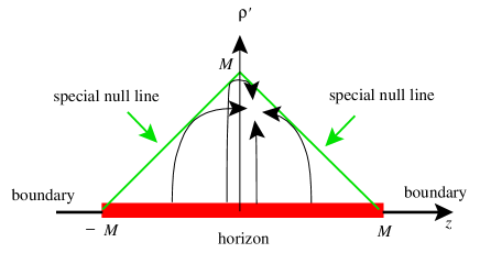
Figure 3: The Weyl representation of the interior of the Schwarzschild black hole naively gives a triangle with base length $2M$ and height $M$. As we illustrate, the triangle interior is covered four times by orbits of $r$ at four different values of $\theta$.

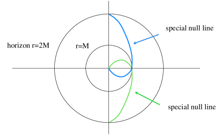
Figure 4: The Weyl null lines for the Schwarzschild black hole correspond to two 3-surfaces which partition $0<r<2M$ into four subregions.

It is clear from (5) that $R_{\pm}$ is positive outside the horizon and there is no difficulty going to negative values inside the horizon. On the other hand in terms of Weyl coordinates, the functions $R_{\pm}=\sqrt{-\rho^{\prime 2}+(z\pm M)^{2}}$ are the square root of a positive number when $\rho^{\prime}<z\pm M$ and imaginary if $\rho^{\prime}>z\pm M$. Clearly, instead of dealing with imaginary values of $R_{\pm}$, the way to go ‘beyond’ the special null line $R_{\pm}=0$ is to keep $\rho^{\prime}<z\pm M$ but use the other square root branch for $R_{\pm}$ as it enters in the Weyl functions $f$ and $\gamma$ by explicitly replacing $R_{\pm}\to-R_{\pm}$. Since we can pass $R_{+}=0$ and/or pass $R_{-}=0$, it is clear that the four different branches of the square root functions differentiate the four copies of the Weyl triangle.

From (3), passing each $R_{\pm}=0$ null line changes the sign of $e^{2\gamma}$ and hence exchanges the timelike and spacelike nature of $\rho^{\prime}$ and $z$. Since the vertical direction on a vertical card always represents time, two of the triangles are drawn turned on their sides, their hypotenuses vertical and so timelike. The four triangles describing the interior of the black hole $0\leq r\leq 2M$ glue together along the special null lines to fit neatly into a square; see Fig. 5. Because of the unfolding of the triangles, the positive $z$-direction on the top triangle (and any attached horizontal cards) points in the opposite direction compared to that on the original horizontal card.

Figure 5: Unfolding the four triangles along the $45^{\circ}$ special null lines for $0<r<2M$, produces a square, V1, of side length $2M$. The horizon is at the bottom and the singularity at the top. We also draw two lines of constant Schwarzschild coordinate $\theta$ and varying $r$.

The upper vertical cards is thus a square of length $2M$. The bottom of the upper card V1 is the black hole horizon which connects to three other cards in a four card junction. The right and left edges of this vertical card correspond to $\theta=0,\pi$ and are the boundaries where $\rho^{\prime}=0$ the $\phi$-circle vanishes. The top edge of the card represents the $r=0$ curvature singularity. The second vertical card V2 is built in analogous fashion except the square is built in a downwards fashion towards negative values of $\rho^{\prime}$. Additionally there is a second horizontal card plane, H2, identical to H1 at negative values of the $\rho$ coordinate attached to the same horizon along $[-M,M]$ on the $z$-axis.

One typically stops the construction of the Schwarzschild spacetime with the above four regions, and considers the $r<0$ part of the metric to be a separate spacetime. However for reasons which become clear when we look at the Reissner-Nordstrøm and Kerr black holes in Sections 3.1.1 and 3.1.4, we continue the card diagram past the singularity and attach two horizontal half-plane corresponding to negative-mass (or $r<0$) universes h3 & h4, and further vertical card above the singularity which is identical to V2. The two new horizontal cards each represent negative mass-universes with no horizon and a naked singularity along $-M\leq z\leq M$. Note that although Penrose diagrams for the $r>0$ and $r<0$ regions of Schwarzschild cannot attach together since the singularity is spacelike in one region and timelike in another, cards can naturally attach at this singularity. The extended card diagram for Schwarzschild, shown in Fig. 6, is an infinite array of repeated cards representing positive (H1,H2) and negative (h3,h4) mass universes and inside-horizon regions.

Figure 6: The extended card diagram for Schwarzschild includes both positive (H1,H2) and negative (h3,h4) mass universes half-planes. Its cross-section for $z=0$ is drawn on the right.

2.2 General properties of card diagrams

Having described the construction of the card diagram for Schwarzschild we now turn to general remarks about these card diagrams. Card diagrams can be constructed in general D-dimensions starting from a generalized Weyl ansatz including the charged cases discussed in Appendix B. Horizontal cards are conformally Euclidean and represent stationary regions. Vertical cards are always conformally Minkowskian and represent regions with ($D-2$) spacelike Killing fields. On a vertical card time is always in the vertical direction and a spacetime point’s causal future lies between $45^{\circ}$ null lines on the card. Weyl’s coordinates certainly go bad at horizons, so these diagrams are not a full replacement for Penrose diagrams at understanding causal structure or particle trajectories. However, it is clear for example from Fig. 1 that two vertical and two horizontal cards attach together in a orthogonal $+$-configuration in precisely the sense of the $\times$-horizon structure of the Penrose diagram.

The prototypical horizon is that of the two Rindler and two Milne wedges of flat space; this spacetime has two horizontal half-plane cards and two vertical half plane cards that meet along the horizon being the whole $z$-axis. Zooming in on a non-extremal horizon of any card diagram yields this Rindler/Milne picture.

A rod endpoint $(\rho,z)=(0,z_{i})$ such as $z=\pm M$ for Schwarzschild is a ‘focus’ for the Weyl diagram and often represents the edge of a black hole horizon or the end of an acceleration horizon on a horizontal card. Generally, multi-black hole Weyl spacetimes depend only on distances to foci, such as $R_{\pm}$ in the case of Schwarzschild [44].

To understand that in general it is natural to change the branch of the distance functions, $R_{i}$, when crossing the special null line that emanates from the foci at $z=z_{i}$, take some Weyl spacetime and imagine moving upwards in a vertical card to meet the special null line where $R_{i}=0$ by increasing time $\rho^{\prime}\geq 0$ for fixed spatial $z$. Rearranging $R_{i}=\sqrt{-\rho^{\prime 2}+(z+z_{i})^{2}}$ as the semi-ellipse

$$R_{i}^{2}+\rho^{\prime 2}=(z+z_{i})^{2},$$

we see that a smooth traversal of this semi-ellipse across $R_{i}=0$ requires a change in the sign of $R_{i}$.

In many of our solutions, special null lines are used to reflect vertical triangular cards to create full, rectangular cards. However, in the Bonnor-transformed S-dihole geometry of [21] as well as double Killing rotated extremal geometries and parabolic representations of the bubble and S-Schwarzschild in Sec. 3.2.3, the special null lines will serve as conformal boundaries at null infinity ${\cal I}^{\pm}$.

Boundaries of cards indicate where the metric coefficient along a Killing (circle) direction vanishes. Which circle vanishes is constant over a connected piece of the boundary, even when the boundary turns a right angle onto a vertical card. Furthermore the periodicity to eliminate conical singularities is constant along connected parts of the boundary. For Schwarzschild, the $\phi$-circle vanishes on both connected boundaries and has periodicity $2\pi$.

Although not a full replacement for understanding causal structure, it is interesting to consider geodesic trajectories on card diagrams. For example when a light ray is incident from a horizontal card onto a horizon (to enter the upper vertical card), it must turn and meet that horizon perpendicularly. It then appears on the vertical card, again perpendicular to the horizon. Only those light rays which go from the lower vertical card to the upper vertical card directly can meet the horizon rod at a non-right angle; these rays would touch the vertex of the $\times$ in a Schwarzschild Penrose diagram. When a light ray on a vertical card hits a boundary where a spacelike circle vanishes, it bounces back at the same angle as drawn on the card relative to the perpendicular.

Spacetimes with a symmetry group larger than the minimal Weyl symmetry can have more than one card diagram representation. Multiple diagrams exist when there is more than one equivalent way to choose $(D-2)$ Killing congruences on the spacetime manifold. Examples we explicitly discuss in Sec. 3.2 are the 4d Witten bubble and the 4d S-Reissner-Nordstrøm (S-RN) which have three card diagrams corresponding to the three types of Killing congruences on dS₂ and ${\bf H}_{2}$. These different card diagrams are associated for example with global, patched, and Poincaré coordinates for dS₂ and the different representations will have different applications and reveal different information. On the other hand the S-Kerr solution, whose card diagram is discussed in Sec. 3.1.4, has symmetry group $U(1)\times{\bf R}$ and its unique card representation looks like the ‘elliptic’ representation of S-RN.

2.2.1 Our deck of cards: The building blocks for Weyl spacetimes

All spacetimes, new and old, in this paper are built from the following card types.

Horizontal cards are always half-planes. They may however have one or more branch cuts which may be taken to run perpendicular to the $z$-axis. Undoing one branch cut leads to a horizontal strip with two boundaries; multiple branch cuts lead to some open subset, with boundary, of a Riemann surface.

Vertical cards may be noncompact: Full planes with or without a pair of special null lines; half-planes with vertical or horizontal (horizon) boundary; or quarter planes at any $45^{\circ}$ orientation. Vertical cards may also be compact: Squares with a pair of special null lines; or 45-45-90 triangles at any $45^{\circ}$ orientation. All horizontal and vertical boundaries represent where a Killing circle vanishes and hence the end of the card. All $45^{\circ}$ null boundaries represent instances of ${\cal I}^{\pm}$.

It is satisfying that for a variety of spacetimes including those in [43, 7], the cards are always of the above rigid types.

There is one basic procedure which can be performed on vertical cards and their corresponding Weyl solutions. It is the analytic continuation $2\gamma\to 2\gamma+i\pi$, which is allowed since $\gamma$ is determined by first order PDEs and $e^{2\gamma}$ is real of either sign on vertical cards. This continuation is equivalent to multiplying the metric by a minus sign and then analytically continuing the $D-2$ Killing directions. For charged generalizations of Weyl solutions (see Appendix B), this procedure does not affect the reality of the 1-form gauge field. We call this analytic continuation a $\gamma$-flip since the way it acts on a card is to geometrically flip it about a $45^{\circ}$ null line (for example, look at the vertical cards in Figs. 19 and 19).

3 Card diagrams

In this section we construct the card diagrams for a wide assortment of solutions including black holes, bubbles and S-branes. The card diagrams are shown to be useful in representing continuous changes in the global spacetime structure such as how Reissner-Nordstrøm black holes change as we take their chargeless and extremal limits. For the superextremal black holes we discuss how to deal with branch points and cuts on horizontal cards. The card diagram also clearly represents the Kerr ring singularity and how traversing the interior of the ring leads to a second asymptotic spacetime. The 5d black ring solution, associated C-metric type solutions and twisted S-branes are also discussed.

Furthermore analytic continuation has an interesting interpretation in terms of card diagrams. We will describe the effect of analytic continuation on the card diagrams by examining two known analytic continuations of the Reissner-Nordstrøm black hole, the charged bubble and the S0-brane which we also call S-RN. These time dependent spacetimes each have three card diagram representation and two are obtained via different analytic continuations in Weyl coordinates. The Witten bubble and S-RN are related to each other by what we call a $\gamma$-flip which is a geometric realization of analytic continuation.

3.1 Black holes

3.1.1 Subextremal $Q^{2}<M^{2}$ Reissner-Nordstrøm black holes

In the usual coordinates the Reissner-Nordstrøm black hole takes the form

$$ds^{2} = -\Big{(}1-{2M\over r}+{Q^{2}\over r^{2}}\Big{)}dt^{2}+\Big{(}1-{2M\over r}+{Q^{2}\over r^{2}}\Big{)}^{-1}dr^{2}+r^{2}(d\theta^{2}+\sin^{2}\theta d\phi^{2})$$ (6)

$$A = Qdt/r$$

Using the coordinate transformation

$$\rho=\sqrt{r^{2}-2Mr+Q^{2}}\sin\theta,\qquad z=(r-M)\cos\theta$$ (7)

we find the Weyl form of Reissner-Nordstrøm black hole

$$ds^{2} = -fdt^{2}+f^{-1}(e^{2\gamma}(d\rho^{2}+dz^{2})+\rho^{2}d\phi^{2})$$ (8)

$$f = \frac{(R_{+}+R_{-})^{2}-4(M^{2}-Q^{2})}{(R_{+}+R_{-}+2M)^{2}}$$

$$e^{2\gamma} = \frac{(R_{+}+R_{-})^{2}-4(M^{2}-Q^{2})}{4R_{+}R_{-}}$$

$$A = -\frac{2Qdt}{R_{+}+R_{-}+2M}$$

$$R_{\pm} = \sqrt{\rho^{2}+(z\pm\sqrt{M^{2}-Q^{2}})^{2}}=r-M\pm\sqrt{M^{2}-Q^{2}}\cos\theta$$

and the card diagram for $Q^{2}<M^{2}$ is shown in Fig. 8. The construction of the card diagram proceeds along similar lines to the Schwarzschild card diagram. There are two adjacent horizontal half-planes, H1 and H2, which represent the positive mass asymptotically flat regions. The outer horizon at $r_{+}=M+\sqrt{M^{2}+Q^{2}}$ is represented in Weyl space as a rod which lies along the $z$-axis for $-\sqrt{M^{2}-Q^{2}}<z<\sqrt{M^{2}-Q^{2}}$. The vertical cards, V1 and V2, are squares of length $2\sqrt{M^{2}-Q^{2}}$ and the diagonal lines connecting opposite corners of the square are special null lines. The top of V2 is the $r_{-}=M-\sqrt{M^{2}-Q^{2}}$ rod which is a four-card inner horizon. The black hole singularity no longer is on the edge of V2 but instead is on the outer boundary of the horizontal h1 and h2 regions, at $\rho^{2}/Q^{2}+z^{2}/M^{2}=1$. Now the singularity is timelike and avoidable from the view of an observer on a vertical card. The rest of those horizontal cards, regions h3 and h4, are $r<0$ or equivalently $M<0$ nakedly singular RN spacetimes.

At each horizon, the card diagram is continued vertically to obtain an infinite tower of cards. In Fig. 8 we show the Penrose diagram for comparison.

Although the chargeless $Q\to 0$ limit is hard to understand from Penrose diagrams, it is easy to understand using the card diagram in Fig. 8; the vertical card expands to a $2M\times 2M$ square and the singularity degenerates to a line segment coinciding with the inner horizon. Regions h1 and h2 disappear so the singularity is now ‘visible’ from V1 and V2 as well as h3 and h4; the singularity is spacelike relative to vertical cards and timelike for horizontal card observers. This achieves the Schwarzschild infinite array of cards in Fig. 6.

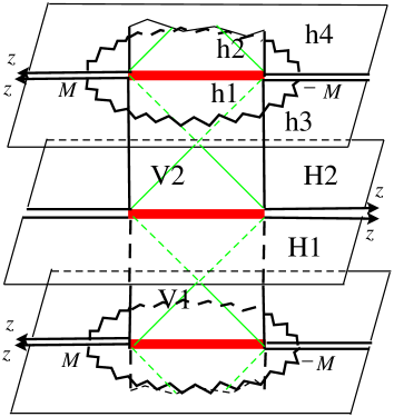
Figure 7: The subextremal Reissner-Nordstrøm card diagram. The ellipse singularity has semimajor axes $z=\pm M$ and $\rho=Q$, and the rod endpoints are the foci on the $z$-axis at $z=\pm\sqrt{M^{2}-Q^{2}}$.

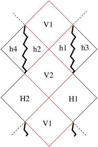
Figure 8: The extended Reissner-Nordstrøm Penrose diagram, including negative mass universes.

3.1.2 Extremal $Q^{2}=M^{2}$ Reissner-Nordstrøm black hole

Starting from the above card diagram we now examine the extremal limit $Q\to\pm M$. In this case the vertical cards which represent the regions between the two horizons get smaller and disappear. When $Q=M$, the horizontal cards are now only attached at point-like extremal-horizons and only half of the horizontal cards remain connected, see Fig. 9. The region near the point-horizons are anti-de Sitter throats although cards themselves cannot adequately depict the throat region. The throat is a ‘connected’ sequence of points on vertically adjacent horizontal cards.

Figure 9: The extremal RN card diagram. The origin of each half-plane is connected to the origin of its two neighbors. This is depicted via a zig-zag line connecting adjacent origins, in analogy to the Poincaré horizons for AdS₂. A side-view $z=0$ cross section is also shown.

To understand how to go across the horizon, it is important to remember that there are special null lines in $r_{-}<r<r_{+}$. In the extremal case the focal distances are equal ($R=R_{+}=R_{-}$) and the null lines $R_{\pm}=0$ degenerate to the origin. So when we pass through the throat to an adjacent $r<M$ horizontal card, the sign changes for all occurrences of $R=\sqrt{\rho^{2}+z^{2}}=r-M$. Half the cards are now absent relative to the subextremal case since we no longer perform analytic continuation to get the vertical card. We can only go from positive real values of $\rho$ to negative values of $\rho$ alternatively. The singularity appears as a semicircle on the $r<M$ cards.

For axisymmetric Majumdar-Papapetrou solutions, this ‘sign change rule’ agrees with that in [22]. Our analysis also applies to non-MP axisymmetric solutions such as the dihole [45, 46, 47].

3.1.3 Superextremal $Q^{2}>M^{2}$ Reissner-Nordstrøm black holes

The superextremal $Q^{2}>M^{2}$ Reissner-Nordstrøm black hole does not have horizons or vertical cards. Its card diagram consists of two horizontal cards, connected along the branch cut $0\leq\rho\leq\sqrt{Q^{2}-M^{2}}$, $z=0$. One card has a semi-ellipse singularity passing through the points $(\rho=0,z=\pm M)$ and $(\rho=Q,z=0)$ (see Fig. 10(a)).

These two horizontal cards are connected in the same sense as a branched Riemann sheet. By choosing Weyl’s canonical coordinates (meaning $Z=\rho+iz$ with $-($Coef$\,dt^{2})($Coef$\,d\phi^{2})=($Re$\,Z)^{2}$), the solution is no longer accurately represented on the horizontal card. This can be seen by examining the coordinate transformation (8) from Schwarzschild coordinates to Weyl coordinates. For fixed $r$ and varying $\theta$, the coordinates from $M<r<\infty$ cover the Weyl plane in semi-ellipses which degenerate to the segment $(0\leq\rho\leq\sqrt{Q^{2}-M^{2}},z=0)$, which serves as a branch cut; and $\rho=\sqrt{Q^{2}-M^{2}}$ is the branch point. The range $-\infty<r<M$ again covers the half-plane with $r=0$ forming an ellipse singularity. Crossing the branch cut means choosing the opposite signs for $R_{\pm}=\sqrt{\rho^{2}-(z\pm i\sqrt{Q^{2}-M^{2}})^{2}}$, and indeed we can think of the superextremal ‘rod’ as being complex-perpendicular to the Weyl $Z$-plane.

This double cover of the Weyl plane can be fixed by taking a holomorphic square root; this preserves the conformally Euclidean character of the card diagram. By choosing a new coordinate $W=\sqrt{Z-\sqrt{Q^{2}-M^{2}}}$, we map both the positive and negative-mass universes into the region $({\rm Im}\,W)^{2}-({\rm Re}\,W)^{2}\leq\sqrt{Q^{2}-M^{2}}$ (see Fig. 10(b)). The image of the $z$-axis boundary is a hyperbola where the $\phi$-circle vanishes. The origin $W=0$ is the image of the branch point and the image of the line segment $(0\leq\rho\leq\sqrt{Q^{2}+M^{2}},z=0)$ is a line connecting the two hyperbolas and intersecting the origin of the $W$-plane. The singular nature of $e^{2\gamma}\propto 1/R_{+}R_{-}\propto 1/|\Delta Z|\propto 1/|W|^{2}$ has been fixed by $e^{2\gamma}dZd\overline{Z}=4|W|^{2}e^{2\gamma}dWd\overline{W}$. Finally the ‘black hole’ singularity is mapped to a curved segment stretching from one hyperbola line to the other, to the left of the branch cut.

Figure 10: (a) The superextremal RN black hole as two half-planes connected along a dashed branch cut line; (b) after conformal transformation to the $W$-plane we obtain a branched, static horizontal card, with two boundaries and one branch point.

Alternatively one can use a Schwarz-Christoffel transformation to map the two universes onto the strip $|{\rm Im}\,W|\leq W_{0}$. This is useful when the horizontal card boundaries are horizons as it allows for multiple horizontal cards to be placed adjacent to each other at the horizons (Fig. 17). This technique of fixing a horizontal card with a branch point will also be used in more complicated geometries such as the hyperbolic representation of S-RN and multi-rod solutions in four and five dimensions [21].

3.1.4 Kerr black hole

Written in Weyl-Papapetrou form, the Kerr black hole is

$$ds^{2} = -f(dt-\omega d\phi)^{2}+f^{-1}(e^{2\gamma}(d\rho^{2}+dz^{2})+\rho^{2}d\phi^{2}),$$ (9)

$$f = \frac{(R_{+}+R_{-})^{2}-4M^{2}+{a^{2}\over M^{2}-a^{2}}(R_{+}-R_{-})^{2}}{(R_{+}+R_{-}+2M)^{2}+{a^{2}\over M^{2}-a^{2}}(R_{+}-R_{-})^{2}},$$

$$e^{2\gamma} = \frac{(R_{+}+R_{-})^{2}-4M^{2}+{a^{2}\over M^{2}-a^{2}}(R_{+}-R_{-})^{2}}{4R_{+}R_{-}},$$

$$\omega = \frac{2aM(M+{R_{+}+R_{-}\over 2})(1-{(R_{+}-R_{-})^{2}\over 4(M^{2}-a^{2})})}{{1\over 4}(R_{+}+R_{-})^{2}-M^{2}+a^{2}{(R_{+}-R_{-})^{2}\over 4(M^{2}-a^{2})})},$$

where $R_{\pm}=\sqrt{\rho^{2}+(z\pm\sqrt{M^{2}-a^{2}})^{2}}=r-M\pm\sqrt{M^{2}-a^{2}}\cos\theta$. The transformation to Boyer-Lindquist coordinates is $\rho=\sqrt{r^{2}-2Mr+a^{2}}\sin\theta$, $z=(r-M)\cos\theta$.

For $a^{2}<M^{2}$ the Kerr black hole card diagram (see Figure 11) is similar to Reissner-Nordstrøm except that the singularity is now a point and lies at $\rho=a$, $z=0$ on each horizontal negative-mass card. The outer and inner ergospheres lie on the positive-and negative-mass cards and are both described by the curve $z^{2}=\alpha^{2}-(\alpha^{2}/a^{2}-1)\rho^{2}-\rho^{4}/a^{2}$ which intersects the rod endpoints at $z=\pm\alpha=\pm\sqrt{M^{2}-a^{2}}$. The boundary of the region with closed timelike curves is also described by a quartic polynomial in Weyl coordinates. Once again the vertical cards have two special null lines where $R_{\pm}$ change sign.

The $r=0$ surface in BL coordinates is a semi-ellipse $\rho^{2}/a^{2}+z^{2}/M^{2}=1$ on the negative-mass card; but it is not a distinguished locus on the card diagram. Attempting to make one loop around the ring in the Kerr-Schild picture clearly does not make a closed loop in Weyl space, whereas two loops in the Kerr-Schild picture will form a single loop around the ring singularity on the card diagram. It is also clear that it is possible to find classical trajectories which avoid the singularity and which safely escape into a second asymptotically flat region.

A card diagram for a charged Kerr-Newman solution can similarly be constructed, with $\alpha=\sqrt{M^{2}-Q^{2}-a^{2}}$.

The extremal Kerr(-Newman) solution has a card diagram like Fig. 9, but the ring singularity is just a point at $z=0$ and $\rho=M$ on negative-mass cards. Again, $R=R_{+}=R_{-}$ and the special null lines degenerate to the origin; crossing the origin (which is a twisted AdS-type throat) entails changing the sign of $R$.

The superextremal Kerr(-Newman) solution is similar to the superextremal RN (Fig. 10(b)) except that the curved-segment singularity is replaced by a point ($z=0$), and the ergospheres map to an $\infty$-looking locus centered at $W=0$.

Figure 11: The Kerr card diagram.

3.1.5 The black ring

The 5d static black ring solution of [23] is

$$ds^{2} =-{F(x)\over F(y)}dt^{2}$$

$$+ {1\over A^{2}(x-y)^{2}}\left[F(x)\Big{(}(y^{2}-1)d\psi^{2}+{F(y)\over y^{2}-1}dy^{2}\Big{)}+F(y)^{2}\Big{(}{dx^{2}\over 1-x^{2}}+{1-x^{2}\over F(x)}d\phi^{2}\Big{)}\right]$$

where $F(x)=1-\mu x$, $F(y)=1-\mu y$, and $0\leq\mu\leq 1$. The coordinates $x$, $y$ are 4-focus (including $\infty$) or C-metric [28, 32, 48, 49] coordinates that parametrize a half-plane of Weyl space $\rho\geq 0$, $-\infty<z<\infty$:

$$\rho = {1\over A(x-y)^{2}}\sqrt{F(x)F(y)(1-x^{2})(1-y^{2})}$$

$$z = {(1-xy)(F(x)-F(y))\over 2A(x-y)^{2}}\ .$$

The foci are on the $z$-axis at $z=\pm\mu/2A$ and $z=1/2A$. The black ring horizon is also on the $z$-axis along $-\mu/2A\leq z\leq\mu/2A$. The $\phi$-circle vanishes along $z\leq-\mu/2A$ and $\mu/2A\leq z\leq 1/2A$, and the $\psi$-circle vanishes along $z\geq 1/2A$. Curves of constant $y$ degenerate to the horizon line segment as $y\to-\infty$, and degenerate to the $(1/2A,\infty)$ ray (better pictured with a conformally equivalent disk) for $y\to-1$. Curves of constant $x$ degenerate to the vanishing $\phi$-circle line segment for $x\to 1$ and to the ray $(-\infty,-\mu/2A)$ for $x\to-1$.

The card diagram is easy to construct and is not much different from the four dimensional Schwarzschild case. Past $y=-\infty$ we can go to $y=+\infty$ and hence imaginary $\rho=i\rho^{\prime}$, and move up a $\mu/A\times\mu/A$ square with two special null lines. At the top of the square, at $y=1/\mu$ we have the curvature singularity. Continuing again to real $\rho$ and running $y$ down to $1$, we map out a (negative-mass) horizontal card. The locus $y=1$ is the ray $z\geq 1/2A$. The space closes off here as the $\psi$-circle vanishes, but we formally continue to illustrate how C-metric coordinates run on noncompact vertical cards—this is useful in several applications, such as the Plebański-Demiański solution [50]. Past $y=1$, we see that for fixed $x$, reducing $y$ down to $x$ makes a topological half-line in a vertical card with a special null line. Then for $-1<y<x$, we traverse another vertical card, which we could attach to our original positive-mass horizontal card along $z>1/2A$ (see Fig. 12).

Figure 12: An extended card diagram for the black ring, where we have continued past $y=$ constant boundaries for $-1\leq x\leq 1$. A $y$-orbit is drawn curving through several cards. Only one of the mirror pairs of vertical and horizontal cards are drawn at each four card junction to avoid too many overlapping figures.

Note that when passing through the black ring horizon at $y=-\infty$, the Weyl conformal factor [23]

$$e^{2\nu}={1+\mu\over 4A}{Y_{23}\over R_{1}R_{2}R_{3}}\sqrt{Y_{12}\over Y_{13}}\sqrt{R_{2}-\zeta_{2}\over R_{3}-\zeta_{3}},$$

stays real; $R_{3}-\zeta_{3}$ and $Y_{13}$ go negative. As we pass the special null lines, explicit appearances of $R_{1}$ and $R_{2}$ in the Weyl functions $e^{2U_{i}}$, $e^{2\nu}$ change sign.

The charged ring of [30] is generated by a functional transformation and hence inherits a card diagram structure. In fact, any geometry with $D-2$ Killing directions written in C-metric coordinates has a card diagram.

3.2 Charged Witten bubbles and S-branes

The Schwarzschild black hole can be analytically continued to two different time-dependent geometries, the Witten bubble of nothing [2] with a dS₂ element and S-Schwarzschild [10, 11, 12] with an ${\bf H}_{2}$ element, and it is instructive to understand how the card diagram changes.

Unlike black hole geometries with their unique card diagrams, these time dependent geometries can have multiple card diagram representations. Both the bubble and S-Schwarzschild have three different card diagram representations corresponding to three different ways to select Killing congruences. These three types of Killing congruences can be understood by representing ${\bf H}_{2}$ as the unit disk (with its conformal infinity being the unit circle). The orientation-preserving isometries of ${\bf H}_{2}$ are those Möbius transformations preserving the disk, $PSL(2,{\bf R})$ [51]. Möbius transformations $z\mapsto{az+b\over cz+d}$ have two complex fixed points, counted according to multiplicity. In the upper half-plane $z=x+i\sigma$ representation, $a$, $b$, $c$, and $d$ are real, so the fixed points are roots of a real quadratic. Hence they may be (i) distinct on the real boundary (hyperbolic), (ii) degenerate on the real boundary (parabolic), or (iii) nonreal complex conjugate pairs, one interior to the upper half-plane ${\bf H}_{2}$ (elliptic). Prototypes of Killing fields are (i) $z\to(1+\epsilon)z$ for the upper half-plane, (ii) $z\to z+\epsilon$ for the upper half-plane; and (iii) $z\to e^{i\epsilon}z$ for the disk $|z|<1$. These are the striped, Poincaré, and azimuthal congruences. In these hyperbolic, parabolic and elliptic representations, the S-Reissner-Nordstrøm (S-RN) and the Witten bubble each have 0, 1, and 2 Weyl foci.

3.2.1 Elliptic representations and extended card diagrams

The bubble of nothing in $D$ dimensions has the interpretation as a semi-classical decay mode of the Kaluza-Klein vacuum. A spatial slice is topologically $S^{D-3}\times{\bf R}^{2}$, where the ${\bf R}^{2}$ is a cigar with the asymptotic-KK $S^{1}$ closing at some fixed $r$, which is an $S^{D-3}$ bubble. As time passes, the bubble increases in size and ‘destroys’ the spacetime. The solution is obtained as an analytic continuation of a black hole and can be generalized to incorporate gauge fields.

The electrically charged bubble of nothing in its elliptic representation is gotten from (6) by sending $t\to ix^{4}$, $\phi\to i\phi$, and to keep the field strength real we need $Q\to-iQ$. The metric is

$$ds^{2}=(1-\frac{2M}{r}-\frac{Q^{2}}{r^{2}})(dx^{4})^{2}+(1-\frac{2M}{r}-\frac{Q^{2}}{r^{2}})^{-1}dr^{2}+r^{2}(d\theta^{2}-\sin^{2}\theta d\phi^{2})$$ (11)

At $\theta=0,\pi$ there are clearly Rindler-type horizons about which we analytically continue $\theta$ and obtain the rest of dS₂, $-d\theta^{2}+\sinh^{2}\theta d\phi^{2}$. These six patches will precisely correspond to the six cards of Fig. 13.

Figure 13: The elliptic representation of the non-singular charged Witten bubble contains two horizons and four special null lines. Here, $\alpha=\sqrt{M^{2}+Q^{2}}$.

Let us now turn to the effect of the analytic continuation of the Reissner-Nordstrøm black hole in Weyl coordinates. In Weyl coordinates, the effect of wick rotating $t\to ix^{4}$ turns the horizon of the Schwarzschild card into an $x^{4}$-boundary, while $\phi\to i\phi$ turns the boundaries on the horizontal card into noncompact acceleration horizons along the rays $|z|\geq M$, $\rho=0$. At the two horizons sending $\theta\to 0\pm i\theta,\pi\pm i\theta$ corresponds to $\rho\to\pm i\rho^{\prime}$ along the $|z|\geq\sqrt{M^{2}+Q^{2}}$ rays. We find vertical noncompact one eighth-plane cards with special null lines along $\rho^{\prime}=z-M$ for $z\geq M$ and $\rho^{\prime}=-M-z$ for $z\leq-M$. Each piece of the plane is a doubly covered triangle and it is necessary to change branches of the function $R_{\pm}$ at the null line, as they appear in (8) to transform the card into a single covered quarter plane card.

The elliptic (and as we will shortly see the hyperbolic) representations of the Witten bubble are simply obtained because their dS₂ Killing congruences are trivially obtained from those on $S^{2}$. Specifically, take the $S^{2}$ embedding into flat space with $Z=\cos\theta$, $X=\sin\theta\cos\phi$, $Y=\sin\theta\sin\phi$. Sending $\phi\to i\phi$ has the effect $Y\to iY^{\prime}$ so the surface becomes $X^{2}-Y^{\prime 2}+Z^{2}=1$ embedded in Minkowski space, or dS₂ with $\phi$ as an elliptic (azimuthal) congruence. On the other hand sending $\theta\to\pi/2+i\theta$, has the effect $Z\to iZ^{\prime}$ giving $X^{2}+Y^{2}-Z^{\prime 2}=1$, which is dS₂ again but with $\phi$ as a hyperbolic (striped) congruence.

Next the S-brane solution of [10, 11, 12]

$$ds^{2}=(1+\frac{2M}{t}-\frac{Q^{2}}{t^{2}})(dx^{4})^{2}-(1+\frac{2M}{t}-\frac{Q^{2}}{t^{2}})^{-1}dt^{2}+t^{2}(d\theta^{2}+\sinh^{2}\theta d\phi^{2})$$ (12)

can also be gotten from (6) by taking $t\to ix^{4}$, $\theta\to i\theta$, $r\to it$, and $M\to iM$. From (7) we see that in Weyl’s coordinates this analytic continuation of RN can be implemented by sending $t\to ix^{4}$, $z\to i\tau$, $M\to iM$, up to a real coordinate transformation.

The card diagram for elliptic S-RN (Fig. 14) has the same structure as the Witten bubble (Fig. 13) except that the 6-segment boundary is now $\theta=0$ where the $\phi$-circle vanishes. The right and left horizons are at $t=t_{\pm}=M\pm\sqrt{M^{2}+Q^{2}}$. The $t=0$ singularity is a hyperbola on the $t_{-}\leq t\leq t_{+}$ horizontal cards parametrized as $(\rho^{\prime},\tau)=(|Q|\sinh\theta,-M\cosh\theta)$. Any $Q\neq 0$ gives the same qualitative diagram. The ‘smaller’ connected universe on the card diagram is the negative-mass version of S-RN. Either sign of the mass gives a universe that is cosmologically singular. The Penrose diagram is given in Fig. 15.

Figure 14: The elliptic S-RN card diagram is similar to Fig. 13 except there is a singularity in the shape of a hyperbola which does not intersect the horizons.

Figure 15: The Penrose diagram for S-RN.

In the limit $Q\to 0$, the hyperbola singularity degenerates to a straight line covering the horizon at $t=0$. The two $t>2M$ vertical cards and two $0<t<2M$ horizontal cards then form a positive-mass S-Schwarzschild, while each $t<2M$ card forms a negative-mass S-Schwarzschild whose singularities begin or end the spacetime.

One can alternatively form the elliptic S-Schwarzschild from the elliptic Witten bubble by performing the $\gamma$-flip on any vertical card. This procedure is immediate; the net continuation from Schwarzschild is $\theta\to i\theta$, $g_{\mu\nu}\to-g_{\mu\nu}$, and avoids $r\to it$, $z\to i\tau$, and $M\to iM$.

Note how the card representation of the S-brane is quite different from the black hole card diagram while the Penrose diagrams of the two spacetimes are nearly just related by ninety degree rotation. This is because the card diagram shows the compact or noncompact $\theta$ direction.

The elliptic form of the card diagrams show that Schwarzschild S-brane, Witten bubble and Schwarzschild solutions have similar structures and in fact they are all related by $\gamma$-flips and trivial Killing continuations. Solutions which are related in this manner may be conveniently drawn together in one diagram which simultaneously displays all of their card diagrams. For example in Fig. 16 the S-Schwarzschild solution comprises regions $1,2,3,4,5$, the Witten bubble regions $4,5,6$, and the Schwarzschild black hole $6,7,8,9,10$. Regions $1,2,10$ correspond to a singular Witten bubble of negative ‘mass.’ In this diagram we also see that the unification of the special null lines as they extend through all three solutions; we can say $R_{+}=0$ is the long $\diagup$-null line and $R_{-}=0$ is the long $\diagdown$-null line.

The charged Reissner-Nordstrøm BH/bubble/S-brane solutions cannot be depicted together on such a diagram because $Q\to iQ$ changes $0<r_{-}<r_{+}$ to $r_{-}<0<r_{+}$. Similar diagrams can be found in [7, 49].

Figure 16: The Schwarzschild black hole, Witten bubble and S-Schwarzschild are all related by $\gamma$-flips and so their (elliptic) card diagrams may be combined into this extended diagram.

3.2.2 Hyperbolic representations and branch points

The charged Witten bubble

$$ds^{2}=\Big{(}1-{2M\over r}-{Q^{2}\over r^{2}}\Big{)}(dx^{4})^{2}+\Big{(}1-{2M\over r}-{Q^{2}\over r^{2}}\Big{)}^{-1}dr^{2}+r^{2}(-d\theta^{2}+\cosh^{2}\theta d\phi^{2})$$ (13)

can alternatively be obtained from the RN black hole (6) by taking $\theta\to\pi/2+i\theta$ and $t\to ix^{4}$, $Q\to-iQ$. Here, $\theta$ plays the role of time and $\theta=0$ is the time where the bubble ‘has minimum size.’ (This statement has meaning if we break $SO(2,1)$ symmetry.) To achieve this in Weyl’s coordinates, we put $z\to i\tau$, $t\to ix^{4}$, $Q\to-iQ$; the resulting space is equivalent to Witten’s bubble by the real coordinate transformation

$$\rho=\sqrt{r^{2}-2Mr-Q^{2}}\,\cosh\theta,\qquad\tau=(r-M)\sinh\theta.$$ (14)

Thus in Weyl coordinates the only difference between the hyperbolic Witten bubble and the elliptic S-RN is putting $M\to iM$. Witten’s bubble universe is represented in Weyl coordinates as a vertical half-plane card, $\rho\geq 0$, $-\infty<\tau<\infty$, where now the $x^{4}$-circle, and not the $\phi$-circle, vanishes at $\rho=0$. This boundary is where the bubble of nothing begins. Note that the vertical card now has Minkowski signature and is conformal to $-d\tau^{2}+d\rho^{2}$. This vertical card does not have special null lines since the foci are at imaginary values $\tau=\pm iM$, and so the spacetime is covered only once by the Schwarzschild coordinates. The bubble does have a rod which is along the imaginary $\tau$ axis and which intersects the card at the $\rho=0$, $\tau=0$ origin. The hyperbolic representation of the charged Witten bubble is therefore just a vertical half-plane. In such a case the card diagrams have just as much causal information as a Penrose diagram and the boundary of the card easily describes the edge of the bubble of nothing.

We obtain a hyperbolic representation for S-RN from (6) by sending $t\to ix^{4}$, $M\to iM$, $r\to ir$, $\theta\to\pi/2+i\theta$, and $\phi\to i\phi$. The fibered directions are now hyperbolic $d{\bf H}_{2}^{2}=d\theta^{2}+\cosh^{2}\theta d\phi^{2}$. In Weyl coordinates, to maintain reality of the solution, we begin with RN (8) and send $t\to ix^{4}$, $\phi\to i\phi$, $M\to iM$, and must explicitly change the branch of the square root introducing the minus sign $R_{-}\to-R_{-}$. This has the interpretation of staying on the same horizontal card and rotating the rod in the complex $z$-plane. The foci are then at ($z=\pm i\sqrt{M^{2}+Q^{2}}$, $\rho=0$) with their special null lines intersecting the real half-plane at $z=0$, $\rho=\sqrt{M^{2}+Q^{2}}$. The half-plane is doubly covered, and we will take $0\leq\rho\leq\sqrt{M^{2}+Q^{2}}$ as the branch cut. The sign change of $R_{-}$ has effectively reversed the roles of $r$ and $\theta$ so that, after undoing the branch cut with say a square-root conformal transformation, $r=r_{+}>0$ is one boundary-horizon and $r=r_{-}<0$ is the other. The hyperbolic angle $\theta$ is unbounded $-\infty<\theta<\infty$.

The doubly-covered half-plane is physically cut into two by the $r=0$ singularity. At each horizon $r=r_{\pm}$ we have a four-card junction; the double half-plane horizontal card meets another mirror copy as well as two vertical cards. The vertical cards are at $\rho\to\pm i\rho^{\prime}$ and $-\infty<z<\infty$ and have no special null lines or other features. A full card diagram is shown in Fig. 17. Note that there are no boundaries of this card diagram where a spacelike Killing circle vanishes.

Figure 17: Hyperbolic S-RN card diagram after transformation to the $W$-plane on the horizontal cards is without boundaries. The singularities are closer to the ${\cal H}_{-}$ horizon than to ${\cal H}_{+}$.

Setting $R_{\pm}=\sqrt{\rho^{2}+(z\pm i\sqrt{M^{2}+Q^{2}})^{2}}$ and $R=R_{+}$, the explicit form of hyperbolic S-RN on the horizontal card is

$$ds^{2} = -f(dx^{4})^{2}+f^{-1}(e^{2\gamma}(d\rho^{2}+dz^{2})+\rho^{2}d\phi^{2}),$$ (15)

$$f = {M^{2}+Q^{2}-({\rm Im}\,R)^{2}\over({\rm Im}\,R+M)^{2}},$$

$$e^{2\gamma} = {M^{2}+Q^{2}-({\rm Im}\,R)^{2}\over|R|^{2}},$$

$$A = {Q\,dx^{4}\over{\rm Im}\,R+M}.$$

We can arrive at this spacetime in a simpler way. Take the RN black hole and analytically continue to get the hyperbolic charged Witten bubbles. These universes are nonsingular for $r\geq r_{+}$ or $r\leq r_{-}$. They have boundaries at $r=r_{\pm}$ where the $x^{4}$-circle vanishes. Now, turn these universes on their sides with the $\gamma$-flip. This allows us to decompactify $x^{4}$ and $r=r_{\pm}$ are now Milne horizons—we are looking precisely at the vertical cards of Fig. 17, and they are connected in a card diagram by an $r_{-}\leq r\leq r_{+}$ card which is now accessible. We see that generally, vertical half-plane cards parametrized in spherical prolate fashion with no special null lines, when turned on their sides, connect to branched horizontal cards.

The $Q\to 0$ limit (hyperbolic S-Schwarzschild) of the card diagram is easy to picture: The singularities of Fig. 17 collapse onto the $r=r_{-}$ horizon.

One may wonder what happens if we take $z\to i\tau$, on the horizontal card for hyperbolic S-RN, and achieves a vertical card sandwiched between special null lines at $\rho=\sqrt{M^{2}+Q^{2}}+|\tau|$. This must unfold to give a vertical plane with two intersecting special null lines. This card diagram structure is discussed in [21, 43].

3.2.3 Parabolic representations

There is a third way to put a Killing congruence on ${\bf H}_{2}$ or dS₂ using parabolic or Poincaré coordinates. Parametrizing hyperbolic space (Euclideanized AdS₂) as $ds^{2}=\sigma^{2}dx^{2}+{d\sigma^{2}\over\sigma^{2}}$, and keeping the Schwarzschild S-brane coordinate $r$ and the usual $x^{4}$ we get a Poincaré Weyl representation of S-RN spacetime [8, 10, 11]. It is

$$ds^{2} = f(dx^{4})^{2}-f^{-1}(e^{2\gamma}(-d\rho^{\prime 2}+dz^{2})+\rho^{\prime 2}dx^{2}),$$ (16)

$$A = Qdx^{4}/r,$$

$$f = (1-2M/r-Q^{2}/r^{2}),$$

$$e^{2\gamma} = {r^{2}-2Mr-Q^{2}\over\sigma^{2}(M^{2}+Q^{2})},$$

$$\rho^{\prime} = \sigma\sqrt{r^{2}-2Mr-Q^{2}},$$

$$z = \sigma(r-M).$$

In this Weyl representation, $\rho^{\prime}$ is timelike on $r\geq r_{+}$ vertical cards which are noncompact $45^{\circ}$ wedges, $0\leq\pm\rho^{\prime}<z$. This connects along $z>0$ to an $r_{-}\leq r\leq r_{+}$ horizontal card; $r\leq r_{-}$ vertical cards attaches to $z<0$. So this is similar to the elliptic representation of S-RN, except the line segment $-\sqrt{M^{2}+Q^{2}}<z<\sqrt{M^{2}+Q^{2}}$ has collapsed and the special null lines are now conformal null infinity (Fig. 19). The singularity on the horizontal card is particularly easy to describe in these coordinates. On the first horizontal card it is on a ray $z/\rho=-M/Q$ and on the second card it is on a ray $z/\rho=M/Q$.

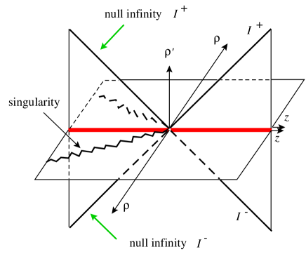
Figure 18: The parabolic card diagram representation for S-Reissner-Nordstrøm. The $45^{\circ}$ vertical lines represent null infinity.

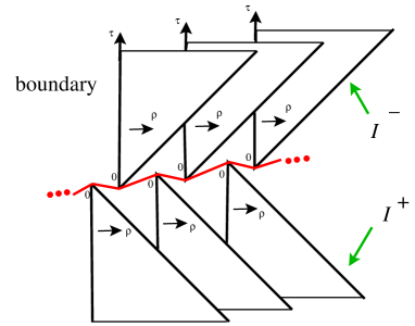
Figure 19: The parabolic representation of the Witten bubble contains an infinite number of $45^{\circ}$ wedge vertical cards pointing up and down with each wedge joined to two others at the tip in a dS₂ fashion.

If we take the $r\geq r_{+}$ (or $r\leq r_{-}$) $45^{\circ}$ wedges and turn them on their sides via the $\gamma$-flip, we get the parabolic version of the $r\geq r_{+}$ (or $r\leq r_{-}$) charged Witten bubble. The line which used to be the horizon in the S-brane card diagram becomes a boundary which is the ‘minimum volume’ sphere, at $\rho=0$. Time is now purely along the $\tau$ direction as in the hyperbolic Witten bubble. The special null line is still ${\cal I}^{\pm}$ since $\rho=|\tau|$ corresponds to $r\to\infty$. The vertex of the triangular card is not the end of the spacetime. These wedge cards only represent $\sigma>0$ and so the card diagram should be extended to $\sigma<0$. The card diagram is an infinite array of $45^{\circ}$ wedge cards pointing up and an infinite number pointing down. The vertex of each upward card is attached to its nearest two downward neighbors (one to the left and one to the right), in the dS₂ fashion as shown in Figure 19. One can identify cards so only needs one upward and one downward card with two attachments. Although this card diagram is not the most obvious representation of the Witten bubble, it is useful in understanding the S-Kerr solution of the next subsection as well as the more complicated S-dihole ${\cal U}$, ${\cal U}_{\pm}$ universes of [21].

3.3 S-Kerr

The twisted S-brane [17], see also [18], is also known as S-Kerr, and it is another example of a nonsingular time-dependent solution. Twisted S-branes describe the decay of unstable massive strings. They can be obtained from the Kerr black hole using the following card diagram method. Double Killing continue $t\to ix^{4}$, $\phi\to i\phi$ to achieve a ${\cal K}_{+}$ bubble solution, go to the vertical card via $\theta\to i\theta$, then perform a $\gamma$-flip to achieve S-Kerr. S-Kerr has symmetry group $U(1)\times{\bf R}$ and therefore has a unique card diagram. For the parameter range $a^{2}<M^{2}$ there are horizons and the card diagram structure is that of the elliptic bubble (Fig. 13). The foci are at $z=\pm\sqrt{M^{2}-a^{2}}$. There is an ergosphere and CTC region on the horizontal card and has the same qualitative shape as it does for the Kerr black hole diagram. In comparison, the Penrose diagram showing (variably twisted) $x^{4}$ and the Boyer-Lindquist coordinate $r$ is shown in Fig. 20.

Figure 20: Subextremal $a^{2}<M^{2}$ S-Kerr Penrose diagram. V_± map to vertical cards of positive and negative ‘mass,’ while all H diamonds give identical horizontal cards. It is possible to identify cards (say, every other H diamond) so there are only a finite number of regions in the spacetime.

Figure 21: The extremal $a^{2}=M^{2}$ (left) and superextremal $a^{2}>M^{2}$ (right) S-Kerr Penrose diagrams.

In the extremal limit $\pm a\to M$, $\theta$-orbits on the vertical card shift up relative to the special null line, and any fixed ($r$, $\theta$) point is sent above the null line. The region below the null line disappears in this limit and the horizontal card collapses to a point. Furthermore, those geodesics in the upper-right card can only reach the lower-left card (and the same with upper-left and lower-right), splitting the universe into connected $45^{\circ}$ wedges just like the parabolic representation for the Witten bubble (Fig. 19), where the connections are dS₂-like twisted throats.

The case $a^{2}>M^{2}$ for S-Kerr does not have horizons and can be represented as a single vertical half-plane card with $\rho\geq 0$ and with no special null lines. Just like the hyperbolic Witten bubble, superextremal S-Kerr can be turned on its side with the $\gamma$-flip, to yield a new spacetime [43]. In the limit where $|a|\to\infty$, the $\theta$-orbits flatten out on the card, and the solution becomes flat space.

The Penrose diagrams for extremal and superextremal S-Kerr are given in Fig. 21.

4 Discussion

In this paper we have examined and extended the utility of the Weyl Ansatz through the construction of an associated Weyl card diagram. Weyl coordinates are an excellent choice for clearly understanding geometric features and so drawing the card diagram is useful. The card diagram conveniently captures most of the interesting properties of a spacetime including its singularities, horizons, and some aspects of its causal structure and null infinity. Card diagrams for families of solutions such as charged and rotating black holes (and bubbles and S-branes) share similar features and can change continuously. They are useful in keeping track of various analytic continuations and mentally partitioning complicated spacetimes into simpler regions. The only technical issues that seem to arise and which we resolved dealt with branches of Weyl distance square-root functions, special null lines on vertical cards, and branched horizontal cards.

Here we summarize the solutions in this paper. The card diagrams correctly capture the different regions of the charged Reissner-Nordstrøm black hole and its various charged and chargeless limits, and its negative mass complement. We also analyzed the Kerr black hole and its singularity structure. In particular the safe passage through the interior of the ring to the second asymptotic universe through $r=0$ is clearly depicted.

The Witten bubbles and S-branes each have three card diagrams representations corresponding to the three different choices of Killing congruences on dS₂ or ${\bf H}_{2}$. The elliptic representations had two foci and six cards. S-RN had a cosmological singularity on the horizontal card splitting the card diagram into two connected universes, whereas the charged bubbles have the same card structure but are nonsingular. The hyperbolic representations have no foci: the bubble is a simple vertical half-plane card and hyperbolic S-RN has a branched horizontal card which we fixed by a conformal mapping of the half-plane. Finally the parabolic representation of the bubble was an infinite array of $45^{\circ}$ triangle wedges connected pointwise while S-RN had a 6-card butterfly shape. This parabolic representation showcased special null lines serving as null infinity.

S-Reissner Nordstrøm can be obtained from the bubble in two ways. One may start with the bubble and analytically continue $M\to iM$ in Weyl coordinates. In this case the hyperbolic/elliptic representation of the bubble maps to the elliptic/hyperbolic representation of the S-brane. We also found that these two solutions can be related by what we called the $\gamma$-flip, which is conveniently visualized as a flip of the associated cards about a null line. This procedure maintains the number of Weyl foci on the card and so maps the elliptic/parabolic/hyperbolic bubble to the elliptic/parabolic/hyperbolic S-brane. The $\gamma$-flip provides a simple and geometric way to relate Schwarzschild with its two analytic continuations, the bubble of nothing and the S-brane. In fact spacetimes related by $\gamma$-flips can be simultaneously drawn together in a complexified $r\theta$ (or $\rho,z$) spacetime diagram.

Just as we used the $\gamma$-flip to turn the hyperbolic Witten bubble on its side and got hyperbolic S-RN, we can take the vertical half-plane card diagrams for the Kerr bubble, dihole wave, superextremal S-Kerr and superextremal S-dihole and apply the $\gamma$-flip to yield new spacetimes. These new solutions will be described in [43].

The card diagram formalism can be further generalized; the recently developed Weyl-Papapetrou formalism [28] for $D\geq 5$ will yield card diagrams and 5d Kerr-related solutions will appear in [43]. Furthermore card diagrams do not require Weyl’s canonical coordinates. Spacetimes with Weyl-type symmetry and yet where Weyl’s procedure fails algebraically can still admit card diagrams. An example is the inclusion of a nonzero cosmological constant $\Lambda$, where a $\gamma$-flip changes the sign of $\Lambda$. Card diagrams for pure (A)dS_D space for $D=4,5$ are presented in [7]. Constant-curvature black holes obtained by quotienting [52] will also have card diagrams. We hope that our methods, and their further generalizations, will have even greater applicability than to the multitude of spacetimes already discussed herein.

Appendix A Perturbed bubbles and S-branes

The chargeless Schwarzschild black hole is easily perturbed as a Weyl solution by adding more rod-horizons, to form Israel-Khan arrays. We can use these solutions to smoothly perturb the Witten bubble in two different ways and also the S-Schwarzschild in two different ways. Addition of charge can be done via Weyl’s electrification method [21, 24, 53].

The analytic continuation in Weyl space to obtain the hyperbolic Witten bubble is precisely the same as in [16], except here the Schwarzschild rod crosses $z=0$. Even-in-$z$ Israel-Khan arrays where no rod crosses $z=0$ can be analytically continued to gravitational wave solutions sourced by imaginary black holes, ie rods at imaginary time. We can thus generalize the Witten bubble by adding additional waves by symmetrically placing more rods in addition to the one which crosses $z=0$. We dub such an array the ‘hyperbolic-perturbed Witten bubble.’ As these additional rods are made to cover more of the $z$-axis and are brought closer and closer to the principal rod, the deformed Witten bubble solution hangs longer with a minimum-radius $\phi$-circle. In the limit where rods occupy the entire $z$-axis, we get a static flat solution, which is Minkowski 3-space times a fixed-circumference $\phi$-circle.

The hyperbolic-perturbed Witten bubble can be turned on its side, yielding a hyperbolic-perturbed S-Schwarzschild. It has the card diagram structure of Fig. 17.

We can also perturb S-Schwarzschild by adding rods before analytically continuing $z\to i\tau$, $M\to iM$. We dub this the ‘elliptic-perturbed S-Schwarzschild.’ It is different than hyperbolic-perturbed S-Schwarzschild, and has the card diagram structure of Fig. 14. Turned on its side, it yields an elliptic-perturbed Witten bubble, with the card diagram structure of Fig. 13. It is different than the hyperbolic-perturbed Witten bubble.

In any of the cases, we can choose to analytically continue the mass parameters of the additional rods or not. Additionally, we can displace some rods in the imaginary $z$-direction which affects the $\tau$-center of their disturbance. If we do everything in an even fashion, i.e. we respect ${\rm Im}\,\tau\to-{\rm Im}\,\tau$, the resulting geometry (at real $\tau$) will be real. In particular, rotating a rod at $z>0$ counterclockwise means rotating its image at $z<0$ clockwise. We see in the discussion of the 2-rod example [21] that there may be several choices for branches.

The card diagram techniques allow us to easily construct these two inequivalent families of perturbed Witten bubble and perturbed S-Schwarzschild solutions. These and other multi-rod, S-dihole, and infinite-periodic-universe solutions are described in [21] and cannot be easily described or understood without Weyl coordinates and the construction and language of card diagrams. The nontrivial $z\to i\tau$ continuation is essential.

Appendix B Appendix: Electrostatic Weyl formalism

The formalism of [23] can be extended for general $D$ to include an electrostatic potential. This is somewhat surprising since the electromagnetic energy-momentum tensor

$$T_{\mu\nu}=F_{\mu\rho}F_{\nu}{}^{\rho}-{1\over 4}g_{\mu\nu}F^{2}$$

is traceless only in $D=4$ and so Einstein’s equations are more complicated. Nevertheless, a cancellation does occur and one may sum the diagonal Killing frame components of the Ricci tensor to achieve a harmonic condition.

Follow the notation of [23] and add a 1-form potential $A(Z,\overline{Z})dt$ where $t=x^{1}$ is timelike ($\epsilon_{1}=-1$) and all other $x^{i}$, $i=2,\ldots,D-2$ are spacelike (with $\epsilon_{i}=+1$). The metric takes the form

$$ds^{2}=-e^{2U_{1}}dt^{2}+\sum_{i=2}^{D-2}e^{2U_{i}}(dx^{i})^{2}+e^{2C}dZd\overline{Z},$$

from which we extract the frame metric

$$g_{\hat{\mu}\hat{\nu}}={\rm diag}(-1,+1,\ldots,+1)\oplus\left[\begin{array}[]{cc}0&1/2\\ 1/2&0\end{array}\right].$$

For $F=dA$ we have $F_{\hat{Z}\hat{t}}=-F_{\hat{t}\hat{Z}}=\partial A\,e^{-U_{1}-C}$ and $F_{\hat{\overline{Z}}\hat{t}}=-F_{\hat{t}\hat{\overline{Z}}}=\overline{\partial}A\,e^{-U_{1}-C}$, all other components vanishing. We compute $F^{2}=-8\partial A\overline{\partial}A\,e^{-2U_{1}-2C}$ and

$$T_{\hat{t}\hat{t}} = 2\partial A\overline{\partial}A\,e^{-2U_{1}-2C}$$

$$T_{\hat{i}\hat{i}} = 2\partial A\overline{\partial}A\,e^{-2U_{1}-2C}\quad(i\neq 1)$$

$$T_{\hat{Z}\hat{Z}} = -(\partial A)^{2}e^{-2U_{1}-2C}$$

$$T_{\hat{\overline{Z}}\hat{\overline{Z}}} = \overline{T_{\hat{Z}\hat{Z}}}$$

$$T_{\hat{Z}\hat{\overline{Z}}} = 0.$$

The field equations are $R_{\hat{\mu}\hat{\nu}}-{1\over 2}g_{\hat{\mu}\hat{\nu}}R=T_{\hat{\mu}\hat{\nu}}$; taking the trace, we get

$$R=-{4(D-4)\over D-2}\partial A\overline{\partial}A\,e^{-2U_{1}-2C}$$

and Einstein’s equations are then

$$R_{\hat{\mu}\hat{\nu}}=T_{\hat{\mu}\hat{\nu}}-{2(D-4)\over D-2}g_{\hat{\mu}\hat{\nu}}\partial A\overline{\partial}A\,e^{-2U_{1}-2C}.$$ (17)

Form the sum $\sum_{i=1}^{D-2}R_{\hat{i}\hat{i}}\epsilon_{i}$; the right side of (17) gives

$$(D-4)2\partial A\overline{\partial}A\,e^{-2U_{1}-2C}-{2(D-4)\over D-2}(D-2)\partial A\overline{\partial}A\,e^{-2U_{1}-2C}=0.$$

Hence (following (2.4)-(2.5) of [23]) we get

$$\partial\overline{\partial}\exp\left(\sum_{i=1}^{D-2}U_{i}\right)=0,$$

the Weyl harmonic condition.

One can add magnetostatic potentials along spatial Killing directions as well. We skip remaining details and give the equations. Let us assume $x^{1}$ is timelike and $x^{i}$ are spacelike for $i=2,\ldots,D-2$, the potential is $A_{\it 1}=\sum_{i=1}^{D-2}A_{i}dx^{i}$, and the metric is $ds^{2}=-e^{2U_{1}}(dx^{1})^{2}+\sum_{i=2}^{D-2}e^{-2U_{i}}(dx^{i})^{2}+e^{2\nu}(d\rho^{2}+dz^{2})$ and $w=\rho+iz$, $\partial_{w}={1\over 2}(\partial_{\rho}-i\partial_{z})$. Einstein’s equations are

$$\Delta U_{1} = {1\over 2}\Big{(}\sum_{i=1}^{D-2}(\nabla A_{i})^{2}e^{-2U_{i}}+{D-4\over D-2}\sum_{i=1}^{D-2}(\nabla A_{j})^{2}e^{-2U_{i}},$$

$$\Delta U_{k} = {1\over 2}\Big{(}-(\nabla A_{1})^{2}e^{-2U_{1}}-(\nabla A_{k})^{2}e^{-2U_{k}}+\sum_{i\neq k,1}(\nabla A_{i})^{2}e^{-2U_{i}}$$

$$\qquad-{D-4\over D-2}\sum_{i\neq 1}(\nabla A_{i})^{2}e^{-2U_{i}}+{D-4\over D-2}(\nabla A_{1})^{2}e^{-2U_{1}}\Big{)},$$

and

$$\partial_{w}\sum_{i=1}^{D-2}\nu=-2\rho(\sum_{i<j}\partial_{w}U_{i}\partial_{w}U_{j}+{(\partial_{w}A_{1})^{2}e^{-2U_{1}}\over 2}-\sum_{i=2}^{D-2}{(\partial_{w}A_{i})^{2}\over 2}e^{-2U_{i}}).$$

Maxwell’s equations are

$$\nabla\cdot\big{(}\nabla A_{i}e^{-2U_{i}}\big{)}.$$

All Laplacians and divergences are with respect to a flat 3d axisymmetric auxiliary space with coordinates $\rho,z$.

References

- [1]
- [2] E. Witten, “Instability Of The Kaluza-Klein Vacuum,” Nucl. Phys. B 195, 481 (1982).
- [3] O. Aharony, M. Fabinger, G. T. Horowitz and E. Silverstein, “Clean time-dependent string backgrounds from bubble baths,” JHEP 0207, 007 (2002) [arXiv:hep-th/0204158].
- [4] D. Birmingham and M. Rinaldi, “Bubbles in anti-de Sitter space,” Phys. Lett. B 544, 316 (2002) [arXiv: hep-th/0205246].
- [5] V. Balasubramanian and S. F. Ross, “The dual of nothing,” Phys. Rev. D 66, 086002 (2002) [arXiv: hep-th/0205290].
- [6] A. Biswas, T. K. Dey and S. Mukherji, “R-charged AdS bubble,” arXiv:hep-th/0412124.
- [7] D. Astefanesei and G. C. Jones, “S-branes and (anti-)bubbles in (A)dS space,” arXiv:hep-th/0502162; JHEP, to appear.
- [8] M. Gutperle and A. Strominger, “Spacelike branes,” JHEP 0204, 018 (2002) [arXiv:hep-th/0202210].
- [9] A. Sen, “Rolling Tachyon,” JHEP 0204, 048 (2002), [arXiv:hep-th/0203211]; “Tachyon Matter,” JHEP 0207, 065 (2002), [arXiv:hep-th/0203265]; “Field Theory of Tachyon Matter,” Mod. Phys. Lett. A17, 1797 (2002), [arXiv:hep-th/0204143]; “Time Evolution in Open String Theory,” JHEP 0210, 003 (2002), [arXiv:hep-th/0207105].
- [10] C. M. Chen, D. V. Gal’tsov and M. Gutperle, “S-brane solutions in supergravity theories,” Phys. Rev. D 66, 024043 (2002) [arXiv:hep-th/0204071].
- [11] M. Kruczenski, R. C. Myers and A. W. Peet, “Supergravity S-branes,” JHEP 0205, 039 (2002) [arXiv:hep-th/0204144].
-
[12]
-
J. E. Wang, “Spacelike and time dependent branes from DBI,” JHEP 0210, 037 (2002) [arXiv:hep-th/0207089],
-
C. P. Burgess, F. Quevedo, S. J. Rey, G. Tasinato and I. Zavala, “Cosmological spacetimes from negative tension brane backgrounds,” JHEP 0210, 028 (2002) [arXiv:hep-th/0207104].
-
-
[13]
-
A. Strominger, “Open string creation by S-branes,” Cargèse 2002, Progress in string, field and particle theory, 335, [arXiv:hep-th/0209090];
-
B. Chen, M. Li and F. L. Lin, “Gravitational radiation of rolling tachyon,” JHEP 0211, 050 (2002), [arXiv:hep-th/0209222];
-
C. P. Burgess, P. Martineau, F. Quevedo, G. Tasinato and I. Zavala C., “Instabilities and particle production in S-brane geometries,” JHEP 0303, 050 (2003), [arXiv:hep-th/0301122];
-
F. Leblond and A. W. Peet, “SD-brane gravity fields and rolling tachyons,” JHEP 0304, 048 (2003), [arXiv:hep-th/0303035];
-
N. Lambert, H. Liu and J. Maldacena, “Closed strings from decaying D-branes,” arXiv:hep-th/0303139.
-
- [14] N. Ohta, “Intersection rules for S-branes,” Phys. Lett. B 558, 213 (2003) [arXiv:hep-th/0301095].
- [15] A. Maloney, A. Strominger and X. Yin, “S-brane thermodynamics,” JHEP 0310, 048 (2003) [arXiv:hep-th/0302146].
- [16] G. C. Jones, A. Maloney and A. Strominger, “Non-singular solutions for S-branes,” Phys. Rev. D 69, 126008 (2004) [arXiv:hep-th/0403050].
- [17] J. E. Wang, “Twisting S-branes,” JHEP 0405, 066 (2004) [arXiv:hep-th/0403094].
- [18] G. Tasinato, I. Zavala, C. P. Burgess and F. Quevedo, “Regular S-brane backgrounds,” JHEP 0404, 038 (2004) [arXiv:hep-th/0403156].
- [19] H. Lü and J. F. Vázquez-Poritz, “Non-singular twisted S-branes from rotating branes,” JHEP 0407, 050 (2004) [arXiv:hep-th/0403248].
- [20] M. Gutperle and W. Sabra, “S-brane solutions in gauged and ungauged supergravities,” Phys. Lett. B 601, 73 (2004) [arXiv:hep-th/0407147].
- [21] G. C. Jones and J. E. Wang, “Weyl card diagrams and new S-brane solutions of gravity,” arXiv:hep-th/0409070.
- [22] R. C. Myers, “Higher Dimensional Black Holes In Compactified Space-Times,” Phys. Rev. D 35, 455 (1987).
- [23] R. Emparan and H. S. Reall, “Generalized Weyl solutions,” Phys. Rev. D 65, 084025 (2002) [arXiv:hep-th/0110258].
- [24] H. Weyl, Ann. Phys. (Leipzig) 54, 117 (1917).
- [25] R. Emparan and E. Teo, “Macroscopic and microscopic description of black diholes,” Nucl. Phys. B 610, 190 (2001) [arXiv:hep-th/0104206].
- [26] C. Charmousis and R. Gregory, “Axisymmetric metrics in arbitrary dimensions,” Class. Quant. Grav. 21 (2004) 527 [arXiv:hep-th/0306069].
-
[27]
-
A. Papapetrou, Ann. Physik 12 (1953) 309;
-
A. Papapetrou, Ann. Inst. H. Poincaré A 4 (1966) 83.
-
- [28] T. Harmark, “Stationary and axisymmetric solutions of higher-dimensional general relativity,” Phys. Rev. D 70, 124002 (2004) [arXiv:hep-th/0408141].
- [29] R. Emparan and H. S. Reall, “A rotating black ring in five dimensions,” Phys. Rev. Lett. 88, 101101 (2002) [arXiv:hep-th/0110260].
- [30] H. Elvang, “A charged rotating black ring,” Phys. Rev. D 68, 124016 (2003) [arXiv:hep-th/0305247].
- [31] H. Elvang and R. Emparan, “Black rings, supertubes, and a stringy resolution of black hole non-uniqueness,” JHEP 0311, 035 (2003) [arXiv:hep-th/0310008].
- [32] R. Emparan, “Rotating circular strings, and infinite non-uniqueness of black rings,” JHEP 0403, 064 (2004) [arXiv:hep-th/0402149].
- [33] H. Elvang, R. Emparan, D. Mateos and H. S. Reall, “A supersymmetric black ring,” Phys. Rev. Lett. 93, 211302 (2004) [arXiv:hep-th/0407065].
- [34] H. Elvang, R. Emparan, D. Mateos and H. S. Reall, “Supersymmetric black rings and three-charge supertubes,” Phys. Rev. D 71, 024033 (2005) [arXiv:hep-th/0408120].
- [35] H. Elvang, R. Emparan and P. Figueras, “Non-supersymmetric black rings as thermally excited supertubes,” JHEP 0502, 031 (2005) [arXiv:hep-th/0412130].
- [36] W. Israel, K. A. Khan, “Collinear Particles and Bondi Dipoles in General Relativity,” Nuovo Cim. 33, 3611 (1964).
- [37] M. A. Melvin, “Pure Magnetic and Electric Geons,” Phys. Lett. 8 (1), 65 (1964).
- [38] F. Dowker, J. P. Gauntlett, G. W. Gibbons and G. T. Horowitz, “The Decay of magnetic fields in Kaluza-Klein theory,” Phys. Rev. D 52, 6929 (1995) [arXiv:hep-th/9507143].
-
[39]
-
M. S. Costa and M. Gutperle, “The Kaluza-Klein Melvin solution in M-theory,” JHEP 0103, 027 (2001) [arXiv:hep-th/0012072],
-
M. Gutperle and A. Strominger, “Fluxbranes in string theory,” JHEP 0106, 035 (2001) [arXiv:hep-th/0104136].
-
- [40] R. Emparan and M. Gutperle, “From p-branes to fluxbranes and back,” JHEP 0112, 023 (2001) [arXiv:hep-th/0111177].
- [41] L. Cornalba and M. S. Costa, “A new cosmological scenario in string theory,” Phys. Rev. D 66, 066001 (2002) [arXiv:hep-th/0203031].
- [42] Siklos, S. T. C. “Two completely singularity-free NUT space-times,” Phys. Lett. A 59, 173 (1976).
- [43] G. C. Jones and J. E. Wang, in preparation.
- [44] N. R. Sibgatullin, Oscillations and Waves in Strong Gravitational and Electromagnetic Fields, Springer-Verlag, Berlin, Heidelberg 1991. (Originally published Nauka, Moscow 1984.)
- [45] W. B. Bonnor, “An Exact Solution of the Einstein-Maxwell Equations Referring to a Magnetic Dipole,” Zeitschrift für Physik 190, 444 (1966).
- [46] S. Chandrasekhar and B. C. Xanthopoulos, “Two Black Holes Attached To Strings,” Proc. Roy. Soc. Lond. A 423, 387 (1989).
- [47] R. Emparan, “Black diholes,” Phys. Rev. D 61, 104009 (2000) [arXiv:hep-th/9906160].
- [48] W. B. Bonnor, “The Sources of the Vacuum -Metric,” Gen. Rel. Grav. 15 (6) 535 (1983).
-
[49]
-
J. Bičák and V. Pravda, “Spinning C metric: Radiative space-time with accelerating, rotating black holes,” Phys. Rev. D 60, 044004 (1999) [arXiv: gr-qc/9902075];
-
V. Pravda and A. Pravdová, “Boost rotation symmetric space-times: Review,” Czech. J. Phys. 50, 333 (2000) [arXiv: gr-qc/0003067].
-
- [50] J. F. Plebański and M. Demiański, “Rotating, charged, and uniformly accelerating mass in general relativity,” Annals of Phys. 98, 98 (1976).
- [51] K. Matsuzaki and M. Taniguchi, Hyperbolic Manifolds and Kleinian Groups, Oxford University Press, New York, 1998.
-
[52]
-
M. Bañados, C. Teitelboim and J. Zanelli, “The Black hole in three-dimensional space-time,” Phys. Rev. Lett. 69, 1849 (1992) [arXiv:hep-th/9204099].
-
M. Bañados, M. Henneaux, C. Teitelboim and J. Zanelli, “Geometry of the (2+1) black hole,” Phys. Rev. D 48, 1506 (1993) [arXiv:gr-qc/9302012].
-
S. minneborg, I. Bengtsson, S. Holst and P. Peldán, “Making Anti-de Sitter Black Holes,” Class. Quant. Grav. 13, 2707 (1996) [arXiv:gr-qc/9604005].
-
M. Bañados, “Constant curvature black holes,” Phys. Rev. D 57, 1068 (1998) [arXiv:gr-qc/9703040].
-
S. Holst and P. Peldán, “Black holes and causal structure in anti-de Sitter isometric spacetimes,” Class. Quant. Grav. 14, 3433 (1997) [arXiv:gr-qc/9705067].
-
M. Bañados, A. Gomberoff and C. Martínez, “Anti-de Sitter space and black holes,” Class. Quant. Grav. 15, 3575 (1998) [arXiv:hep-th/9805087].
-
R.-G. Cai, “Constant curvature black hole and dual field theory,” Phys. Lett. B 544, 176 (2002) [arXiv:hep-th/0206223].
-
- [53] S. Fairhurst and B. Krishnan, “Distorted black holes with charge,” Int. J. Mod. Phys. D 10, 691 (2001) [arXiv:gr-qc/0010088].