DSF–4–2005

SISSA 37/2005/FM

The beat of a fuzzy drum:

Fuzzy Bessel functions for the disc

Fedele Lizzi, Patrizia Vitale and Alessandro Zampini^∗

Dipartimento di Scienze Fisiche, Università di Napoli Federico II
and INFN, Sezione di Napoli
Monte S. Angelo, via Cintia, 80126 Napoli, Italy
fedele.lizzi, patrizia.vitale, alessandro.zampini@na.infn.it

^∗ present address: S.I.S.S.A. - Scuola Internazionale Superiore di Studi Avanzati -
via Beirut 2-4, 34014 Trieste, Italy

zampini@sissa.it

The fuzzy disc is a matrix approximation of the functions on a disc which preserves rotational symmetry. In this paper we introduce a basis for the algebra of functions on the fuzzy disc in terms of the eigenfunctions of a properly defined fuzzy Laplacian. In the commutative limit they tend to the eigenfunctions of the ordinary Laplacian on the disc, i.e. Bessel functions of the first kind, thus deserving the name of fuzzy Bessel functions.

1 Introduction

Noncommutative geometry [2, 3, 4, 5] has suggested the introduction of fuzzy spaces, namely the approximation of the abelian algebra of functions on an ordinary space, with a finite rank matrix algebra, which preserves the symmetries of the original space, at the price of noncommutativity. The first formalization of the idea of a fuzzy space was introduced by Madore [6], for the sphere. In his approach, a fuzzy sphere is a sequence of nonabelian algebras, generated (loosely speaking) by three “noncommutative coordinates” which satisfy $x_{i}x_{i}=1$ and $[x_{i},x_{j}]=\kappa\varepsilon_{ijk}x_{k}$, with $\kappa$ some noncommutativity parameter. The connection with the finite dimensional representations of $SU(2)$ is immediate, and with $\kappa$ proportional to the inverse of the rank of the representation, one can think of recovering functions on the sphere in some limit. This limit has been made rigorous by Rieffel [7] at the level of topological “quantum spaces”, but here we are more interested in the approximations that the fuzzy matrix geometry can give to the space of functions (and hence of fields) defined on some space. This is efficiently done defining “fuzzy spherical harmonics” [8, 9], a basis for the matrix algebra, which in the limit converges to the ordinary spherical harmonics. Field theory on the fuzzy sphere is a very active field of research. A partial list of references is [10].

After the fuzzy sphere, similar approximations for higher dimensional spheres [11], for the torus, based on the noncommutative torus algebra [12, 13], and for projective spaces [14], have also been studied. In previous work [15, 16], we proposed a fuzzy approximations for the algebra of functions on a disc (see also [17, 18]). It is the first example of a fuzzy approximation for a space that classically has a boundary. The space is defined through a suitable truncation of the noncommutative plane. In this paper we examine the spectral properties of the fuzzy Laplacian, finding its eigenvalues and eigenvectors, and comparing them with the exact case and give a direct way to associate, to functions on the disc, their fuzzy counterpart, i.e. to approximate the abelian algebra of functions by a sequence of finite rank matrices. We introduce a basis for the algebra of functions on the fuzzy disc in terms of symbols of the eigenmatrices of the fuzzy approximation to the Laplacian. These symbols are seen to converge, as the rank of the matrices increases, towards a set of functions on the plane which coincide with the ordinary Bessel functions of first kind (eigenfunctions of the ordinary Laplacian with Dirichlet boundary conditions) for points on a plane inside a disc, and to zero for points outside this disc. These are given the name of fuzzy Bessel functions.

The paper is organised as follows. In the next section we review the fuzzy sphere from a perspective which will render easy the generalization to the disc case. The main tool we use is the Weyl-Wigner formalism, and the concept of generalized coherent sates, which we briefly review in appendices A and B respectively. In section 3 we review the fuzzy disc. A Weyl-Wigner isomorphism is introduced in terms of functions on the plane, where noncommutativity is represented by a parameter $\theta$. In this formalization, there is no natural concept of a sequence of finite dimensional Hilbert spaces, or finite rank matrix algebras, therefore a truncation in the algebra of operators is introduced, with respect to a specific basis in the Hilbert space. Constraining the dimension $N$ of the truncation to the noncommutativity parameter, $N\theta=R^{2}$, one obtains then a sequence of finite rank matrices, converging towards an abelian algebra of operators, that approximates functions whose support is concentrated on a disc of radius $R$. On this sequence of states, fuzzy derivatives and a fuzzy Laplacian are defined and the spectral properties of the latter are studied. Then in section 4 we study eigenvalues and eigenvectors and show that they (rather quickly) converge to the ordinary Bessel functions.

2 The fuzzy sphere in the Weyl-Wigner formalism

In this section we present the fuzzy sphere in the general context of the Weyl-Wigner formalism [20, 21, 22]. We first set up an isomorphism between a space of operators and a space of functions on a sphere. Since a sphere is the coadjoint orbit of the group $SU\left(2\right)$, the basic tool to introduce this map is a system of coherent states, specialising the general arguments of appendix B.

To define a system of coherent states consider the unitary irreducible representations for the group $SU\left(2\right)$. On each finite dimensional Hilbert space ${\hbox{\mybb C}}^{N}$, with $N=2L+1$ -here $\left(L=0,1/2,1,3/2\ldots\right)$-, a basis is given by vectors that, in ket notation, are represented as $\left|L,M\right.\rangle$ -with $M=\left(-L,-L+1,\ldots,L-1,L\right)$-. One has:

$$u\,\in\,SU\left(2\right)\,\stackrel{{\scriptstyle\hat{R}^{\left(L\right)}}}{{\mapsto}}\,\mathcal{B}\left({\hbox{\mybb C}}^{N}\right)\ .$$ (2.1)

The matrix elements of this representation are given by:

$$\langle L,M|\hat{R}^{\left(L\right)}\left(u\right)|L,M^{\prime}\rangle=D_{MM^{\prime}}^{L}\left(u\right)\ .$$ (2.2)

These are called Wigner functions [23].

The second step is to fix a fiducial state. One can choose the highest weight in the representation: $|\psi_{0}\rangle=|L,L\rangle$. If the group manifold is parametrised by Euler angles, then $u$ represents a point whose “coordinates” range through $\,\alpha\in\left[\left.0,4\pi\right)\right.\,$,$\,\beta\in\left[\left.0,\pi\right)\right.\,$, $\,\gamma\in\left[\left.0,2\pi\right)\right.\,$. Fixed the fiducial vector, its stability subgroup $H_{\psi_{0}}$ by the $\hat{R}^{\left(L\right)}$ representation is made by elements for which $\beta=0$ (this condition is seen to be valid independently of $N$). Two elements $u$ and $u^{\prime}$ are equivalent if $u^{\dagger}u^{\prime}\in H_{\psi_{0}}$. It is possible to prove that:

$$SU\left(2\right)/H_{\psi_{0}}\approx S^{2}$$ (2.3)

identifying $\theta=\beta$ and $\varphi=\alpha\mod\,2\pi$. Chosen a representative element $\tilde{u}$ in each equivalence class of the quotient, the set of coherent states is defined as:

$$|\theta,\varphi,N\rangle=\hat{R}^{\left(L\right)}\left(\tilde{u}\right)|L,L\rangle\ .$$ (2.4)

The left hand side ket now explicitly depends on $N$, the dimension of the space on which the representation takes place. Projecting on the basis elements, one has:

$$\langle L,M|\theta,\varphi,N\rangle = D_{ML}^{L}\left(\tilde{u}\right)\ ,$$ (2.5)

$$|\theta,\varphi,N\rangle = \sum_{M=-L}^{L}\left({\textstyle\frac{\left(2L\right)!}{\left(L+M\right)!\left(L-M\right)!}}\right)^{1/2}\left(\cos\theta/2\right)^{L+M}\left(\sin\theta/2\right)^{L-M}e^{-i\varphi M}\,|L,M\rangle\ .$$

This set of states is nonorthogonal, and overcomplete ($d\Omega=d\varphi\,\sin\theta\,d\theta$):

$$\langle\theta^{\prime},\varphi^{\prime},N|\theta,\varphi,N\rangle = e^{-iL\left(\varphi^{\prime}-\varphi\right)}\,\left[e^{i\left(\varphi^{\prime}-\varphi\right)}\cos\theta/2\cos\theta^{\prime}/2+\sin\theta/2\sin\theta^{\prime}/2\right]^{2L}\ ,$$

$${1\!\!1} = \frac{2L+1}{4\pi}\int_{S^{2}}\,d\Omega|\theta,\varphi,N\rangle\langle\theta,\varphi,N|\ .$$ (2.6)

Using this set of vectors it is possible to define a map, from the space of operators on a finite dimensional Hilbert space to the space of functions on the sphere $S^{2}$:

$$\hat{A}^{\left(N\right)}\,\in\,\mathcal{B}\left({\hbox{\mybb C}}^{N}\right)\,\approx\,\mathbb{M}_{N}\,\,\, \mapsto \,\,\,A^{\left(N\right)}\,\in\,\mathcal{F}\left(S^{2}\right)\ ,$$

$$A^{\left(N\right)}\left(\theta,\varphi\right)\, = \,\langle\theta,\varphi,N|\hat{A}^{\left(N\right)}|\theta,\varphi,N\rangle\ .$$ (2.7)

This is a way to map every finite rank matrix into a function on a sphere, called the Berezin symbol of the given matrix [19]. Among these operators, there are $\hat{Y}^{\left(N\right)}_{JM}$ whose symbols are the spherical harmonics, up to order $2L$ (here $J=0,1,\ldots,2L$ and $M=-J,\ldots,+J$):

$$\langle\theta,\varphi,N|\hat{Y}^{\left(N\right)}_{JM}|\theta,\varphi,N\rangle\,=\,Y_{JM}\left(\theta,\varphi\right)\ ,$$ (2.8)

these operators are called fuzzy harmonics. The origin of this name must be traced back to the definition, on each finite rank matrix algebra $\mathbb{M}_{N}$, of an operator, in terms of the generators $\hat{L}_{a}^{\left(N\right)}$:

$$\left[\hat{L}_{a}^{\left(N\right)},\hat{L}_{b}^{\left(N\right)}\right]\,=\,i\epsilon_{abc}\hat{L}_{c}^{\left(N\right)}\ ,$$ (2.9)

representing the Lie algebra of the group $SU\left(2\right)$ on the space ${\hbox{\mybb C}}^{N}$:

$$\nabla^{2}\, : \,\mathbb{M}_{N}\,\mapsto\,\mathbb{M}_{N}\ ,$$

$$\nabla^{2}\hat{A}^{\left(N\right)}\, = \,\left[\hat{L}_{s}^{\left(N\right)},\left[\hat{L}_{s}^{\left(N\right)},\hat{A}^{\left(N\right)}\right]\right]\ .$$ (2.10)

This operator is called the fuzzy Laplacian. Its spectrum is given by eigenvalues $\mathcal{L}_{j}=j\left(j+1\right)$, where $j=0,\ldots,2L$, and every eigenvalue has a multiplicity of $2j+1$. The spectrum of the fuzzy Laplacian thus coincides, up to order $2L$, with the one of its continuum counterpart acting on the space of functions on a sphere. The cut-off of this spectrum is of course related to the dimension of the rank of the matrix algebra under analysis. The fuzzy harmonics are the eigenstates of this operator.

Fuzzy harmonics are a basis in each space of matrices $\mathbb{M}_{N}$. They are orthogonal but non normalized and are proportional to the polarization operators $\hat{T}^{\left(N\right)}_{JM}$ defined in terms of the Clebsh-Gordan coefficients for $SU(2)$ [23]:

$$\left[\hat{L}_{\mu}^{\left(N\right)},\hat{T}^{\left(N\right)}_{JM}\right]\, = \,\sqrt{L\left(L+1\right)}\,C^{L\,M+\mu}_{L\,M\ 1\,\mu}\,\hat{T}^{\left(N\right)}_{LM+\mu}\ ,$$

$$Tr\left[\hat{T}^{\left(N\right)\,\dagger}_{JM}\,\hat{T}^{\left(N\right)}_{J^{\prime}M^{\prime}}\right] = \delta_{JJ^{\prime}}\delta_{MM^{\prime}}\ ,$$

$$\hat{T}^{\left(N\right)\,\dagger}_{JM} = \left(-1\right)^{M}\hat{T}^{\left(N\right)}_{J-M}\ .$$ (2.11)

the proportionality being:

$$\hat{Y}^{\left(N\right)}_{JM}=\frac{J!}{\left(2lJ\right)^{J}}\left[\frac{\left(2l+J+1\right)!}{4\pi\left(2l-J\right)!}\right]^{1/2}\hat{T}^{\left(N\right)}_{JM}\ ,$$ (2.12)

from which:

$$\>{\rm Tr}\,\left[\hat{Y}^{\left(N\right)\,\dagger}_{JM}\hat{Y}^{\left(N\right)}_{J^{\prime}M^{\prime}}\right]=\left(\frac{J!}{\left(2lJ\right)^{J}}\right)^{2}\left(\frac{\left(2l+J+1\right)!}{4\pi\left(2l-J\right)!}\right)\delta_{JJ^{\prime}}\delta_{MM^{\prime}}\ .$$ (2.13)

Using this basis, an element $\hat{F}^{\left(N\right)}$ belonging to $\mathbb{M}_{N}$ can be expanded as:

$$\hat{F}^{\left(N\right)}=\sum_{J=0}^{2L}\sum_{M=-J}^{J}\,F^{\left(N\right)}_{JM}\,\hat{Y}^{\left(N\right)}_{JM}\ ,$$ (2.14)

with coefficients

$$F^{\left(N\right)}_{JM}=\frac{\>{\rm Tr}\,\left[\hat{Y}^{\left(N\right)\dagger}_{JM}\,\hat{F}^{\left(N\right)}\right]}{\>{\rm Tr}\,\hat{Y}^{\left(N\right)\dagger}_{JM}\hat{Y}^{\left(N\right)}_{JM}}\ .$$ (2.15)

A Weyl-Wigner map can be defined simply mapping spherical harmonics into fuzzy harmonics:

$$\hat{Y}^{\left(N\right)}_{JM}\,\,\Leftrightarrow\,\,Y_{JM}\left(\theta,\varphi\right)\ .$$ (2.16)

This map clearly depends on the dimension $N$ of the space on which fuzzy harmonics are realized. It can be linearly extended by:

$$\hat{F}^{\left(N\right)}=\sum_{J=0}^{2L}\sum_{M=-J}^{J}\,F^{\left(N\right)}_{JM}\hat{Y}^{\left(N\right)}_{JM}\,\,\,\,\leftrightarrow\,\,\,\,F^{\left(N\right)}\left(\theta,\phi\right)=\sum_{J=0}^{2L}\sum_{M=-J}^{+J}F_{JM}^{\left(N\right)}Y_{JM}\left(\theta,\phi\right).$$ (2.17)

This is a Weyl-Wigner isomorphism and it can be used to define a fuzzy sphere. Given a function on a sphere, if it is square integrable with respect to the standard measure $d\Omega$, then it can be expanded in the basis of spherical harmonics:

$$f\left(\theta,\varphi\right)=\sum_{J=0}^{\infty}\sum_{M=-J}^{J}\,f_{JM}\,Y_{JM}\left(\theta,\varphi\right).$$ (2.18)

Now consider the set of “truncated” functions:

$$f^{\left(N\right)}\left(\theta,\varphi\right)=\sum_{J=0}^{2L}\sum_{M=-J}^{J}\,f_{JM}\,Y_{JM}\left(\theta,\varphi\right)\ .$$ (2.19)

This is a vector space, but it is no more an algebra, with the standard definition of sum and pointwise product of two functions, as the product of two spherical harmonics of order say $2L$ has spherical components of order larger than $2L$. We have indeed:

$$\left(Y_{J^{\prime}M^{\prime}}Y_{J^{\prime\prime}M^{\prime\prime}}\right)\left(\theta,\varphi\right)=\sum_{J=\left|J^{\prime}-J^{\prime\prime}\right|}^{J=\left|J^{\prime}+J^{\prime\prime}\right|}\sum_{M=-J}^{J}\sqrt{\frac{\left(2J^{\prime}+1\right)\left(2J^{\prime\prime}+1\right)}{4\pi\left(2J+1\right)}}\,C^{J0}_{J^{\prime}0\,J^{\prime\prime}0}\,C^{JM}_{J^{\prime}M^{\prime}\,J^{\prime\prime}M^{\prime\prime}}\,Y_{JM}\left(\theta,\varphi\right)$$ (2.20)

in terms of Clebsh-Gordan coefficients for $SU\left(2\right)$. If these truncated functions are mapped, via the Weyl-Wigner procedure, into matrices:

$$f^{\left(N\right)}\left(\theta,\varphi\right)\,\mapsto\,\hat{f}^{\left(N\right)}=\sum_{J=0}^{2L}\sum_{M=-J}^{+J}\,f_{JM}\hat{Y}^{\left(N\right)}_{JM}\ ,$$ (2.21)

then this set of truncated functions is given the vector space structure of $\mathbb{M}_{N}$. But $\mathbb{M}_{N}$ is even a nonabelian algebra. Invertibility of this association (2.21) enables to define, in the set of the truncated functions on the sphere, a non abelian product, isomorphic to that of matrices:

$$\left(f^{\left(N\right)}*g^{\left(N\right)}\right)\left(\theta,\varphi\right)=\sum_{J=0}^{2L}\,\sum_{M=-J}^{+J}\,\frac{Tr\left[\hat{f}^{\left(N\right)}\hat{g}^{\left(N\right)}\hat{Y}_{JM}^{\left(N\right)\,\dagger}\right]\,Y_{JM}\left(\theta,\varphi\right)}{\>{\rm Tr}\,\hat{Y}^{\left(N\right)\dagger}_{JM}\hat{Y}^{\left(N\right)}_{JM}}\ .$$ (2.22)

The Weyl-Wigner map (2.17) has been used to make each set of truncated functions a non abelian algebra $\mathcal{A}^{\left(N\right)}\left(S^{2},*\right)$, isomorphic to $\mathbb{M}_{N}$. The product of two fuzzy harmonics can be obtained in term of the 6j-symbols from the product of two polarization operators [8]

$$\hat{T}^{\left(N\right)}_{J^{\prime}M^{\prime}}\hat{T}^{\left(N\right)}_{J^{\prime\prime}M^{\prime\prime}}=\sum_{J}\left(-1\right)^{2L+J}\sqrt{\left(2J^{\prime}+1\right)\left(2J^{\prime\prime}+1\right)}\left\{\begin{array}[]{ccc}{\scriptstyle J^{\prime}}&{\scriptstyle J^{\prime\prime}}&{\scriptstyle J}\\ {\scriptstyle L}&{\scriptstyle L}&{\scriptstyle L}\end{array}\right\}C^{JM}_{J^{\prime}M^{\prime}\,J^{\prime\prime}M^{\prime\prime}}\hat{T}^{\left(N\right)}_{JM}\ .$$ (2.23)

These algebras can be seen as formally generated by matrices which are the images of the norm $1$ vectors in ${\hbox{\mybb R}}^{3}$, i.e. points on a sphere. They are mapped into multiples of the generators $\hat{L}_{a}^{\left(N\right)}$ of the Lie algebra:

$$\frac{x_{a}}{\parallel\vec{x}\parallel}\,\mapsto\,\hat{x}_{a}^{\left(N\right)}\,\,\,\,\,\,\,\,\left[\hat{x}_{a}^{\left(N\right)},\hat{x}_{b}^{\left(N\right)}\right]=\frac{2i\varepsilon_{abc}}{\sqrt{N^{2}-1}}\,\hat{x}_{c}^{\left(N\right)}\ .$$ (2.24)

The commutation rules satisfied by generators of the algebras in the sequence $\mathcal{A}^{\left(N\right)}\left(S^{2},*\right)$ make it intuitively clear that the limit for $N\,\rightarrow\,\infty$ of this sequence is an abelian algebra. This is the reason why this sequence is called fuzzy sphere.

3 The fuzzy disc

In the previous section, the fuzzy sphere has been introduced via the Weyl-Wigner formalism, which makes use of the fact that the 2-dimensional sphere is the coadjoint orbit of the compact group $SU\left(2\right)$. Compactness of the group brought to a natural definition of a sequence of finite dimensional Hilbert spaces, and a natural identification of the dimension of these spaces as a cut-off index for a suitable expansion of a generic function on the sphere. Properties of the sphere as an orbit of that group made it possible to formalize every point of the sphere as a coherent state, defined on each of those finite dimensional spaces carrying the UIRR’s. So the map between operators (finite rank matrices) and functions on the sphere has been naturally introduced via the Berezin procedure, and has been refined stressing the role of the fuzzy Laplacian operator in the definition of fuzzy harmonics as a basis in the set $\mathbb{M}_{N}$. Moreover, compactness of the group played a fundamental role in the rigorous analysis of the convergence performed by Rieffel [7].

To approach the problem of defining a fuzzy approximation to the disc, it would be natural then to analyse the possibility that the disc were a coadjoint orbit for a Lie group. If this were the case, it would be possible to introduce a system of coherent states labelled by its points, and some sort of Berezin map [19]. However this approach meets some troubles. The group from which it is possible to define a system of coherent states in correspondence with points of a disc is $SU\left(1,1\right)$, but it is non compact, so its UIRR’s are not realized on finite dimensional Hilbert spaces. Hence, there is no intrinsic concept of a cut-off index, the would be dimension of the fuzzification, in this context. In [15] the problem has been circumvented using coherent states for the Heisenberg-Weyl group and the standard isomorphism in terms of Berezin symbols between operators and functions on the plane. Then a sequence of projections converging to the characteristic function of the disc has been defined. The projections identify a sequence of finite rank matrix algebras which can be endowed with an additional structure, a fuzzy Laplacian, identifying the underlying geometry. In the commutative limit $N\theta=R^{2}$ this geometry is seen to converge to a disc of radius $R$.

It is well known that it is possible to define a basis for the space of functions on the disc in terms of a suitable set of Bessel functions. Since the Weyl-Wigner map for functions on the sphere has been introduced (2.17) mapping spherical harmonics into fuzzy harmonics, we pose the question whether or not it is possible to define a system of fuzzy Bessel functions in terms of finite rank matrices, and then map again continuum Bessel functions into them. Since Bessel functions are defined on the plane, in connection with boundary values problems for Laplacian operators, the noncommutative plane which we are going to revue, together with fuzzy derivations and a fuzzy Laplacian will turn out to be a natural setting to perform the analysis. The final answer to the problem will be given studying the spectral resolution of the fuzzy Laplacian.

3.1 The noncommutative plane as a matrix algebra

The noncommutative plane can be defined using a Weyl-Wigner map, following again the general procedure of Berezin: so the first step will be the definition of a set of generalised coherent states for the Heisenberg-Weyl group, since they are labelled by points of a plane. In this space it will be assumed a system of coordinates of the kind $\left(x,y\right)$ for a point of ${\hbox{\mybb R}}^{2}$; $\theta$ will be a parameter representing an explicit noncommutativity.

With this notation, Heisenberg-Weyl group is a manifold ${\hbox{\mybb R}}^{3}$, whose points are represented by a triple $\left(x,y,\lambda\right)$, with the composition rule:

$$\left(x,y,\lambda\right)\cdot\left(x^{\prime},y^{\prime},\lambda^{\prime}\right)=\left(x+x^{\prime},y+y^{\prime},\lambda+\lambda^{\prime}-\frac{1}{\theta}\left(xy^{\prime}-x^{\prime}y\right)\right)\ .$$ (3.25)

The identity of this group is given by:

$$id_{W}=\left(0,0,0\right)\ ,$$ (3.26)

and the inverse of a generic element is:

$$\left(x,y,\lambda\right)^{-1}=\left(-x,-y,-\lambda\right)\ .$$ (3.27)

Considering the complex plane via $z=x+iy$ and $\overline{z}=x-iy$ the group law becomes:

$$\left(z,\lambda\right)\cdot\left(z^{\prime},\lambda^{\prime}\right)=\left(z+z^{\prime},\lambda+\lambda^{\prime}+\frac{i}{2\theta}\left(\overline{z}z^{\prime}-\overline{z}^{\prime}z\right)\right)\ .$$ (3.28)

The Hilbert space on which representing this group is again the Fock space $\mathcal{F}$ of finite norm complex analytical functions in the $w$ variable where the norm is obtained by the scalar product:

$$\langle f|g\rangle\,\equiv\,\int\,\frac{d^{2}w}{\pi\theta}\,e^{-\bar{w}w/\theta}\,\bar{f}\left(w\right)g\left(w\right)\ ,$$ (3.29)

and an orthonormal basis is given by:

$$\psi_{n}\left(w\right)=\frac{w^{n}}{\sqrt{\theta^{n}n!}}\ .$$ (3.30)

The unitary representation of the Heisenberg-Weyl group is given by operators $\hat{T}\left(z,\lambda\right)\,\in\,Op\left(\mathcal{F}\right)$:

$$\left(\hat{T}f\right)\left(w\right)=e^{i\lambda}e^{-\bar{z}z/2\theta}e^{zw/\theta}f\left(w-\bar{z}\right)\ .$$ (3.31)

Chosen the first basis element $\psi_{0}\left(w\right)$ as the fiducial state, the procedure already outlined gives a coherent state for each point of the complex plane. In the realization of the Fock space as a space of complex analytical functions, a coherent state is then:

$$|z\rangle\,\,\,\rightarrow\,\,\,\psi_{z}\left(w\right)=e^{-\bar{z}z/2\theta}e^{zw/\theta}$$ (3.32)

and, given $\psi_{n}$ an element of the basis already considered:

$$|z\rangle=\sum_{n=0}^{\infty}e^{-\bar{z}z/2\theta}\frac{z^{n}}{\sqrt{n!\theta^{n}}}|\psi_{n}\rangle\ .$$ (3.33)

Such coherent states are non orthogonal, and overcomplete:

$$\langle z|z^{\prime}\rangle = e^{-\left(\left|z\right|^{2}+\left|z^{\prime}\right|^{2}-2\bar{z}z^{\prime}\right)/\theta}\ ,$$

$${1\!\!1} = \int\frac{d^{2}z}{\pi\theta}\,|z\rangle\langle z|\ .$$ (3.34)

On this Hilbert space $\mathcal{F}$, it is possible to introduce a pair of creation-annihilation operators:

$$\left(\hat{a}f\right)\left(w\right) = \theta\frac{df}{dw}$$

$$\left(\hat{a}^{\dagger}f\right)\left(w\right) = wf\left(w\right)\ ,$$ (3.35)

such that:

$$\left[\hat{a},\hat{a}^{\dagger}\right]=\theta\,{1\!\!1},$$ (3.36)

and:

$$\hat{a}|z\rangle=z|z\rangle\ ,$$ (3.37)

so that we can recognize the usual coherent states encountered in quantum mechanics textbooks. In the chosen orthonormal basis, one has:

$$\hat{a}|\psi_{n}\rangle = \sqrt{n\theta}|\psi_{n-1}\rangle$$

$$\hat{a}^{\dagger}|\psi_{n}\rangle = \sqrt{\left(n+1\right)\theta}|\psi_{n+1}\rangle\ ,$$ (3.38)

and therefore one recognizes the basis as the basis of eigenvectors of the number operator $\hat{N}=\hat{a}^{\dagger}\hat{a}$. Note however the unconventional presence $\theta$ in the commutation relation (3.36).

These relations can be extended. A Berezin symbol can be associated to an operator in the Fock space:

$$f\left(\bar{z},z\right)=\langle z|\hat{f}|z\rangle\ .$$ (3.39)

This can be seen as a Wigner map. It can be inverted:

$$\hat{f}=\int\,\frac{d^{2}\xi}{\pi\theta}\,\int\,\frac{d^{2}z}{\pi\theta}\,f\left(z,\bar{z}\right)\,e^{-\left(\bar{z}\xi-\bar{\xi}z\right)/\theta}\,e^{\xi\hat{a}^{\dagger}/\theta}\,e^{-\bar{\xi}\hat{a}/\theta}.$$ (3.40)

This quantization map for functions on a plane can be given an interesting form. To start with, we can restrict to functions which can be written as Taylor series in $\bar{z},z$:

$$f\left(\bar{z},z\right)=\sum_{m,n=0}^{\infty}\,f_{mn}^{Tay}\bar{z}^{m}z^{n}\ .$$ (3.41)

An easy calculation shows that this $f$ is the symbol of the operator:

$$\hat{f}=\sum_{m,n=0}^{\infty}\,f_{mn}^{Tay}\hat{a}^{\dagger m}\hat{a}^{n}\ .$$ (3.42)

More generally we can consider operators written in a density matrix notation:

$$\hat{f}=\sum_{m,n=0}^{\infty}\,f_{mn}|\psi_{m}\rangle\langle\psi_{n}|\ .$$ (3.43)

The Berezin symbol of this operator is the function:

$$f\left(\bar{z},z\right)=e^{-\left|z\right|^{2}/\theta}\sum_{m,n=0}^{\infty}\,f_{mn}\frac{\bar{z}^{m}z^{n}}{\sqrt{m!n!\theta^{m+n}}}\ ,$$ (3.44)

where the relation between the Taylor coefficients $f_{mn}^{Tay}$ and the $f_{mn}$ is

$$f_{lk}=\sum_{q=0}^{\min\left(l,k\right)}\,f_{l-q\,k-q}^{Tay}\,\frac{\sqrt{k!l!\theta^{l+k}}}{q!\theta^{q}}\ ,$$ (3.45)

while the inverse relation is given by:

$$f_{mn}^{Tay}=\sum_{p=0}^{\min\left(m,n\right)}\,\frac{\left(-1\right)^{p}}{p!\sqrt{\left(m-p\right)!\left(n-p\right)!\theta^{m+n}}}\,f_{m-p\,n-p}\ .$$ (3.46)

Equation (3.42) shows that the quantization of a monomial in the variables $z,\bar{z}$ is an operator in $\hat{a},\hat{a}^{{\dagger}}$, formally a monomial in these two noncommuting variables, with all terms in $\hat{a}^{{\dagger}}$ acting at the left side with respect to terms in $\hat{a}$. This ordering is related to the presence, in the quantization map (3.40), of a specific term that, in the standard terminology used for the Weyl-Wigner formalism, is called weight [24]. In fact, restoring real variables  (3.40) can be written as:

$$\hat{f}=\int\,\frac{dadb}{2\pi\theta}\,\int\,\frac{dxdy}{2\pi\theta}\,f\left(x,y\right)\,e^{-\frac{i\left(bx-ay\right)}{\theta}}\,e^{\frac{u\hat{a}^{\dagger}}{\theta}}\,e^{-\frac{\bar{u}\hat{a}}{\theta}}=\int\,\frac{dadb}{2\pi\theta}\,\tilde{f}\left(b,a\right)\,e^{\frac{\left(a^{2}+b^{2}\right)}{8\theta}}\,e^{\frac{\left(u\hat{a}^{{\dagger}}-\bar{u}\hat{a}\right)}{\theta}}\ .$$ (3.47)

with $u=\left(a+ib\right)/2$. The function $\tilde{f}$ is the symplectic Fourier transform of the function $f$. Compared (3.47) with the standard Weyl map [24, 22], the difference is the factor $e^{\left(a^{2}+b^{2}\right)/8\theta}$.

The invertibility of the Weyl map (on a suitable domain of functions on the plane) enables to define a noncommutative product in the space of functions, known as Voros product [25, 26], a variant of the more popular Grönewold-Moyal product [27, 28]:

$$\left(f*g\right)\left(\bar{z},z\right)=\langle z|\hat{f}\hat{g}|z\rangle\ .$$ (3.48)

It is a non local product:

$$\left(f*g\right)\left(\bar{z},z\right)=e^{-\bar{z}z/\theta}\int\,\frac{d^{2}\xi}{\pi\theta}\,f\left(\bar{z},\xi\right)g\left(\bar{\xi},z\right)\,e^{-\bar{\xi}\xi/\theta}e^{\bar{\xi}z/\theta}e^{\bar{z}\xi/\theta}\ .$$ (3.49)

Its asymptotic expansion, on a suitable domain, acquires the form:

$$\left(f*g\right)\left(\bar{z},z\right)=f\,e^{\theta\overleftarrow{\partial}_{\bar{z}}\overrightarrow{\partial}_{z}}\,g,$$ (3.50)

and makes it clear that it is a deformation, in $\theta$, of the pointwise commutative product. Since it is the translation, in the space of functions, of the product in the space of operators, if symbols are expressed in the form (3.44), then the product acquires a matrix form:

$$\left(f*g\right)_{mn}=\sum_{k=0}^{\infty}f_{mk}g_{kn}\ .$$ (3.51)

The space of functions on the plane, with the standard definition of sum, and the product given by the Voros product (3.48), is a nonabelian algebra, a noncommutative plane. This algebra $\mathcal{A}_{\theta}=\left(\mathcal{F}\left({\hbox{\mybb R}}^{2}\right),*\right)$ is isomorphic to an algebra of operators, or, as equation (3.51) suggests, to an algebra of infinite dimensional matrices. A more detailed mathematical analysis of the Moyal algebra, i.e. of the quantum plane, is given in [29] and references therein.

3.2 A sequence of non abelian algebras

A fuzzy space has been presented as a sequence of finite rank matrix algebras converging to an algebra of functions. The meaning of this convergence is formalised as compact quantum metric spaces. In the case of the fuzzy sphere the rank of the matrices involved is the dimension of the Hilbert space on which UIRR’s of the group $SU\left(2\right)$ are realised. In the approach sketched in the last section there is no natural definition of a set of finite dimensional matrix algebras. This is a consequence of the fact that the noncommutative plane has been realised via a Berezin quantization based on coherent states originated by a group, the Heisenberg-Weyl, which is noncompact.

In this context the strategy to obtain finite dimensional matrix algebras is different. $\mathcal{A}_{\theta}$ can be considered, once a basis in the Hilbert space has been chosen, as a matrix algebra made up by formally infinite dimensional matrices. One can define a set of finite dimensional matrix algebras simply truncating $\mathcal{A}_{\theta}$. The notion of truncation is formalised via the introduction of a set of projectors:

$$\hat{P}_{\theta}^{(N)}=\sum_{n=0}^{N}|\psi_{n}\rangle\langle\psi_{n}|$$ (3.52)

in the space of operators. Their symbols are projectors in the algebra $\mathcal{A}_{\theta}$ of the noncommutative plane, in the sense that they are idempotent functions of order $2$ with respect to the Voros product (here $z=re^{i\varphi}$):

$$P_{\theta}^{\left(N\right)}\left(r,\varphi\right) = \sum_{n=0}^{N}\langle z|\psi_{n}\rangle\langle\psi_{n}|z\rangle=e^{-r^{2}/\theta}\sum_{n=0}^{N}\,\frac{r^{2n}}{n!\theta^{n}}$$

$$P_{\theta}^{\left(N\right)}*P_{\theta}^{\left(N\right)} = P_{\theta}^{\left(N\right)}\ .$$ (3.53)

This finite sum can be performed yielding a rotationally symmetric function:

$$P_{\theta}^{\left(N\right)}\left(r,\varphi\right)\,=\,\frac{\Gamma\left(N+1,r^{2}/\theta\right)}{\Gamma\left(N+1\right)}\ .$$ (3.54)

in terms of the ratio of an incomplete gamma function by a gamma function [30]. If $\theta$ is kept fixed, and nonzero, in the limit for $N\,\rightarrow\,\infty$ the symbol $P_{\theta}^{\left(N\right)}\left(r,\varphi\right)$ converges, pointwise, to the constant function $P_{\theta}^{\left(N\right)}\left(r,\varphi\right)=1$, which can be formally considered as the symbol of the identity operator: in this limit one recovers the whole noncommutative plane.

This situation changes if the limit for $N\,\rightarrow\,\infty$ is performed keeping the product $N\theta$ equals to a constant, say $R^{2}$. In a pointwise convergence, chosen $R^{2}=1$:

$$P^{\left(N\right)}_{\theta}\,\,\rightarrow\,\,\,\left[\begin{array}[]{cc}1&r<1\\ 1/2&r=1\\ 0&r>1\end{array}\right]=Id\left(r\right)\ .$$ (3.55)

This sequence of projectors converges to a step function in the radial coordinate $r$, the characteristic function of a disc on the plane. Thus a sequence of subalgebras $\mathcal{A}_{\theta}^{\left(N\right)}$ can be defined by:

$$\mathcal{A}_{\theta}^{\left(N\right)}=P_{\theta}^{\left(N\right)}*\mathcal{A}_{\theta}*P_{\theta}^{\left(N\right)}\ .$$ (3.56)

As it has been said, the full algebra $\mathcal{A}_{\theta}$ is isomorphic to an algebra of operators. What the previous relation says is that $\mathcal{A}_{\theta}^{\left(N\right)}$ is isomorphic to $\mathbb{M}_{N+1}$, the algebra of $\left(N+1\right)$ rank matrices: the important thing is that this isomorphism (this truncation) is obtained via a specific choice of a basis in the Fock space $\mathcal{F}$ on which coherent states for the Heisenberg-Weyl group are realised. The effect of this projection on a generic function is:

$$\Pi^{\left(N\right)}_{\theta}\left(f\right)=f^{\left(N\right)}_{\theta}=P^{\left(N\right)}_{\theta}*f*P^{\left(N\right)}_{\theta}=e^{-\left|z\right|^{2}/\theta}\sum_{m,n=0}^{N}f_{mn}\frac{\bar{z}^{m}z^{n}}{\sqrt{m!n!\theta^{m+n}}}\ .$$ (3.57)

On every subalgebra $\mathcal{A}^{\left(N\right)}_{\theta}$, the symbol $P^{\left(N\right)}_{\theta}\left(r,\varphi\right)$ is then the identity, because it is the symbol of the projector $\hat{P}^{\left(N\right)}=\sum_{n=0}^{N}|\psi_{n}\rangle\langle\psi_{n}|$, which is the identity operator in $\mathcal{A}_{\theta}^{\left(N\right)}$, or, equivalently, the identity matrix in every $\mathbb{M}_{N+1}$.

Note that the rotation group on the plane, $SO\left(2\right)$, acts in a natural way on these subalgebras. Its generator is the truncated number operator $\hat{N}^{(N)}=\sum_{n=0}^{N}\,n\theta|\psi_{n}\rangle\langle\psi_{n}|$. Cutting at a finite $N$ the expansion provides an infrared cutoff. This cutoff is “fuzzy” in the sense that functions in the subalgebra are still defined outside the disc of radius $R$, but are exponentially damped. In general functions are close to their projected version $f^{\left(N\right)}_{\theta}$ if they are mostly supported on a disc of radius $R=\sqrt{N\theta}$, otherwise they are exponentially cut, provided they do not present oscillations of too small wavelength (compared to $\theta$). In this case the projected function becomes very large on the boundary of the disc. More details and examples are in [15, 16].

3.3 Fuzzy derivatives and fuzzy Laplacian

So far the Weyl-Wigner formalism, and the projection procedure, have provided a way to associate to functions on the plane a sequence of finite dimension $\left(N+1\right)\times\left(N+1\right)$ matrices. An appropriate choice of $\theta$, the noncommutativity parameter introduced by the quantization map, and $N$, showed that it is possible to obtain a good approximation of a certain class of functions supported on a disc. The next step is the analysis of the geometry these algebras can formalize. To pursue this task, we need derivations and a Laplacian. The starting point to define the matrix equivalent of the derivations is:

$$\partial_{z}f\, = \,\frac{1}{\theta}\langle z|\left[\hat{f},\hat{a}^{\dagger}\right]|z\rangle\ ,$$

$$\partial_{\bar{z}}f\, = \,\frac{1}{\theta}\langle z|\left[\hat{a},\hat{f}\right]|z\rangle\ .$$ (3.58)

This relation is exact in the full algebra $\mathcal{A}_{\theta}$. Given an operator $\hat{f}$, the derivatives of the symbol $f\left(\bar{z},z\right)$ are related to the symbol of the commutator of $\hat{f}$ with the creation and annihilation operators. A fuzzified version, namely a truncated version, of these operations, can be defined as:

$$\partial_{z}f^{\left(N\right)}_{\theta} \equiv \frac{1}{\theta}\langle z|\hat{P}^{\left(N\right)}_{\theta}\left[\hat{P}^{\left(N\right)}_{\theta}\hat{f}\hat{P}^{\left(N\right)}_{\theta},\hat{a}^{\dagger}\right]\hat{P}^{\left(N\right)}_{\theta}|z\rangle$$

$$\partial_{\bar{z}}f^{\left(N\right)}_{\theta} \equiv -\frac{1}{\theta}\langle z|\hat{P}^{\left(N\right)}_{\theta}\left[\hat{P}^{\left(N\right)}_{\theta}\hat{f}\hat{P}^{\left(N\right)}_{\theta},\hat{a}\right]\hat{P}^{\left(N\right)}_{\theta}|z\rangle\ .$$ (3.59)

It is important to note that this is really a derivation on each $\mathcal{A}^{\left(N\right)}_{\theta}$, that is a linear operation from $\mathcal{A}^{\left(N\right)}_{\theta}$ to itself, satisfying the Leibnitz rule. The way this is achieved in (3.59) goes through the following steps. We first associate to $f^{\left(N\right)}_{\theta}$ a finite rank matrix $\hat{f}^{\left(N\right)}_{\theta}$ which is indeed regarded as embedded in an infinite dimensional one, with all zeroes but $(N+1)\times(N+1)$ elements in the upper left corner: $\hat{f}^{\left(N\right)}_{\theta}=\hat{P}^{\left(N\right)}_{\theta}\hat{f}\hat{P}^{\left(N\right)}_{\theta}$. We then perform the commutator with $\hat{a},~{}\hat{a}^{\dagger}$ realised as infinite dimensional matrices. This operation yields an infinite dimensional matrix with all zeroes but $(N+2)\times(N+2)$ elements in the upper left corner, so that we have to project back to $\mathbb{M}_{N+1}$ to obtain a properly defined derivation. Finally, we consider the symbol.

As an example let us calculate the derivatives of the fuzzified coordinate functions $z$ and $\bar{z}$. From the definition, $z$, $\bar{z}$ are respectively the symbol of the annihilation and creation operators, which can be written as:

$$\hat{a}\, = \,\sum_{s=0}^{\infty}\,\sqrt{\left(s+1\right)\theta}|\psi_{s}\rangle\langle\psi_{s+1}|$$

$$\hat{a}^{\dagger}\, = \,\sum_{k=0}^{\infty}\,\sqrt{\left(k+1\right)\theta}|\psi_{k+1}\rangle\langle\psi_{k}|.$$ (3.60)

Projection into $\mathbb{M}_{N+1}$ gives:

$$\hat{a}^{\left(N\right)}_{\theta}=\sum_{s=0}^{N-1}\,\sqrt{\left(s+1\right)\theta}|\psi_{s}\rangle\langle\psi_{s+1}|\ .$$ (3.61)

According to (3.59), to perform the derivative with respect to $z$, we have to consider:

$$\left[\hat{a}^{\left(N\right)}_{\theta},\hat{a}^{\dagger}\right] = \theta\left[|\psi_{0}\rangle\langle\psi_{0}|+\sum_{s=1}^{N-1}|\psi_{s}\rangle\langle\psi_{s}|-N|\psi_{N}\rangle\langle\psi_{N}|\right]$$ (3.62)

$$= \theta\left[\sum_{s=0}^{N-1}|\psi_{s}\rangle\langle\psi_{s}|-N|\psi_{N}\rangle\langle\psi_{N}|\right]$$

$$= \theta\left[\sum_{s=0}^{N}|\psi_{s}\rangle\langle\psi_{s}|-\left(1+N\right)|\psi_{N}\rangle\langle\psi_{N}|\right].$$

The first term of the sum is the projector onto the first $N+1$ basis elements, whose symbol is the identity in $\mathcal{A}^{\left(N\right)}_{\theta}$. It is worth noting that this commutator has no terms ’outside’ the space we are considering, namely there are no components on density matrices of order greater than $N+1$: this means that in this case there is no need to project it on $\mathbb{M}_{N+1}$. The symbol yields then:

$$\partial_{z}\left(z^{\left(N\right)}_{\theta}\right)=e^{-Nr^{2}}\left[\sum_{s=0}^{N}\,\frac{r^{2s}N^{s}}{s!}\,-\,\frac{N+1}{N!}r^{2N}N^{N}\right]\ .$$ (3.63)

In the limit of $N\rightarrow\infty$ the first term is the characteristic function for the disc, while the second converges to a factor $\pi\delta\left(r-1\right)$. This factor is a radial $\delta$ selecting the value $r=1$ with respect to the Lebesgue measure on the plane:

$$\lim_{N\rightarrow\infty}\partial_{z}\left(z^{\left(N\right)}_{\theta}\right)=Id\left(r\right)-\pi\delta\left(r-1\right)\ .$$ (3.64)

To calculate the derivative of $\bar{z}$ with respect to $z$ one needs to consider:

$$\hat{a}^{\dagger\left(N\right)}_{\theta}=\sum_{k=0}^{N-1}\,\sqrt{\left(k+1\right)\theta}|\psi_{k+1}\rangle\langle\psi_{k}|$$

and the commutator:

$$\left[\hat{a}^{\dagger\left(N\right)}_{\theta},\hat{a}^{\dagger}\right]=-\theta\sqrt{N\left(N+1\right)}|\psi_{N+1}\rangle\langle\psi_{N}|\ .$$ (3.65)

Unlike the previous example this operator must be projected back to the algebra $\mathbb{M}_{N+1}$, and upon considering the symbol we finally have:

$$\partial_{\bar{z}}\left(z^{\left(N\right)}_{\theta}\right)=0\ .$$ (3.66)

Let us come to the definition of the Laplacian operator. In the spirit of noncommutative geometry it is this additional structure which carries the information about the geometry of the space underlying $\mathcal{A}_{\theta}$. In facts, we can say we have succeeded in fuzzifying the disc only if we have been able to define a fuzzy Laplacian whose spectrum approaches that of the ordinary Laplacian on the disc when $N\rightarrow\infty$.

Starting from the exact expressions:

$$\nabla^{2}\,f(\bar{z},z)=4\partial_{\bar{z}}\partial_{z}f=\frac{4}{\theta^{2}}\langle z|\left[\hat{a},\left[\hat{f},\hat{a}^{\dagger}\right]\right]|z\rangle$$ (3.67)

it is possible to define, in each $\mathcal{A}^{\left(N\right)}_{\theta}$:

$$\nabla^{2}_{\left(N\right)}\,\hat{f}^{\left(N\right)}_{\theta}\equiv\frac{4}{\theta^{2}}\hat{P}^{\left(N\right)}_{\theta}\left[\hat{a},\left[\hat{P}^{\left(N\right)}_{\theta}\hat{f}\hat{P}^{\left(N\right)}_{\theta},\hat{a}^{\dagger}\right]\right]\hat{P}^{\left(N\right)}_{\theta}\ .$$ (3.68)

The image of the element of the truncated algebra:

$$\hat{f}^{\left(N\right)}_{\theta}=\sum_{a,b=0}^{N}\,f_{ab}|\psi_{a}\rangle\langle\psi_{b}|$$

is then:

$$\nabla^{2}_{\left(N\right)}\,f^{\left(N\right)}_{\theta} = \,4N\,\left[\sum_{s=0}^{N-1}\,\sum_{b=0}^{N-1}\,f_{s+1,b+1}\sqrt{\left(s+1\right)\left(b+1\right)}|\psi_{s}\rangle\langle\psi_{b}|\right.+$$ (3.69)

$$-\sum_{s=0}^{N}\,\sum_{b=0}^{N}\,f_{sb}\left(s+1\right)|\psi_{s}\rangle\langle\psi_{b}|\,-\,\sum_{s=0}^{N-1}\,f_{0,s+1}\left(s+1\right)|\psi_{0}\rangle\langle\psi_{s+1}|+$$

$$+\sum_{s=0}^{N-1}\,\sum_{b=0}^{N-1}\,f_{sb}\sqrt{\left(s+1\right)\left(b+1\right)}|\psi_{s+1}\rangle\langle\psi_{b+1}|+$$

$$-\left.\sum_{s=0}^{N-1}\,\sum_{b=0}^{N-1}\,f_{s+1,b+1}\,\left(b+1\right)|\psi_{s+1}\rangle\langle\psi_{b+1}|\,\right].$$

The eigenvalues of this Laplacian can be numerically calculated. They are seen to converge to the spectrum of the continuum one for functions on a disc, with boundary conditions on the edge of the disc of Dirichlet homogeneous kind [31]. All eigenvalues are negative, and their modules $\lambda$ solve the implicit equation:

$$J_{n}\left(\sqrt{\lambda}\right)=0\ ,$$ (3.70)

where $n$ is the order of the Bessel functions. In particular, those related to $J_{0}$ are simply degenerate, the others are doubly degenerate: so there is a sequence of eigenvalues labelled by $\lambda_{n,k}$ where $n$ is the order of the Bessel function and $k$ indicates that it is the $k^{th}$ zero of the function. The eigenfunctions of this continuum operator are:

$$\Phi_{n,k}=e^{in\varphi}\left(\frac{\sqrt{\lambda_{\left|n\right|,k}}r}{2}\right)^{|n|}\sum_{s=0}^{\infty}\frac{\left(-\lambda_{|n|,k}\right)^{s}}{s!\left(|n|+s\right)!}\left(\frac{r}{2}\right)^{2s}=e^{in\varphi}J_{|n|}\left(\sqrt{\lambda_{\left|n\right|,k}}r\right)\ .$$ (3.71)

with $n$ integer number and $|n|$ its absolute value. This is a way to write the eigenfunctions in a compact form, taking into account the degeneracy of eigenvalues for $|n|\geq 1$.

The spectrum of the fuzzy Laplacian is in good agreement with the spectrum of the continuum case, even for low values $N$ of the dimension of truncation, as can be seen in figure 1.

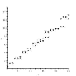
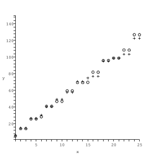
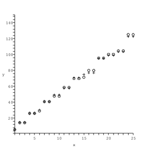
Figure 1: Comparison of the first eigenvalues of the fuzzy Laplacian (circles) with those of the continuum Laplacian (crosses) on the domain of functions with Dirichlet homogeneous boundary conditions. The orders of truncation are $N=10,20,30$.

It is interesting to note that with this definition of Laplacian (3.68) we correctly reproduce the pattern of non degenerate and double degenerate eigenvalues. The difference with the case of the spectrum of the fuzzy Laplacian for the fuzzy sphere is that now the ”fuzzy spectrum” is both a cut-off and an approximation of the continuum spectrum. It is a cut-off because, of course, it is a finite rank operator. It is an approximation because it has been defined using a formalism whose building blocks are related to a noncompact group, namely the Heisenberg-Weyl, whose generators have no finite dimensional realization.

4 Fuzzy Bessel functions

In this section we introduce a basis on the fuzzy disc. As we have already noticed in the introduction, we cannot use representation theory, which in the case of the fuzzy sphere yields the fuzzy harmonics, because there is no compact group whose homogeneous space is the disc. But we have a well defined Laplacian for each $\mathcal{A}_{\theta}^{\left(N\right)}$. Therefore we may answer the problem looking at the eigenfunctions of this fuzzy Laplacian.

4.1 Spectral properties of the Laplacian

The fuzzy Laplacians (3.68) are a family of operators mapping each algebra $\mathcal{A}^{\left(N\right)}_{\theta}$ into itself with the explicit action (3.69). Considering $\mathcal{A}^{\left(N\right)}_{\theta}$ as a $\left(N+1\right)^{2}$ dimensional vector space, a density matrix $|\psi_{a}\rangle\langle\psi_{b}|$ is a basis element for it, with $a,b\,\in\,\left(0,\ldots,N\right)$. Equation (3.69) can be specified:

$$\nabla^{2}_{\left(N\right)}\left(|\psi_{a}\rangle\langle\psi_{b}|\right) = 4N\,\hat{P}^{\left(N\right)}_{\theta}\left(\sqrt{ab}\,|\psi_{a-1}\rangle\langle\psi_{b-1}|\right.+$$

$$\left.-\left(a+b+1\right)\,|\psi_{a}\rangle\langle\psi_{b}|\,+\,\sqrt{\left(a+1\right)\left(b+1\right)}\,|\psi_{a+1}\rangle\langle\psi_{b+1}|\right)\hat{P}^{\left(N\right)}_{\theta}\ .$$

The action of the projector operator is to cut away some of the components of the right side image for $a=0,N$ and for $b=0,N$. It is important to note that, chosen an integer $n=a-b$, the fuzzy Laplacian maps basis elements with the same $n$ onto themselves, as $n$ ranges through $\left(-N,\ldots,+N\right)$. In the matrix representation of $\mathcal{A}^{\left(N\right)}_{\theta}$, the number $n$ fixes the diagonal to which the element $|\psi_{a}\rangle\langle\psi_{b}|$ belongs. The equation (4.1) then shows that the fuzzy Laplacian maps each diagonal subspace of $\mathbb{M}_{N+1}$ into itself. This property simplifies the study of the spectral properties of the fuzzy Laplacian. The analysis of these spectral properties will be performed restricting the operator to each of its stability subspaces.

To understand the meaning of this integer $n$, go back to the eigenfunctions of the continuum Laplacian on a disc with Dirichlet homogeneous boundary conditions (3.71). Eigenfunctions $\Phi_{n,k}$ are defined on the real plane, so they can be mapped into operators on the whole Hilbert space via the Weyl map introduced before (3.40). The continuum eigenfunctions (3.71) with a fixed nonnegative $n$, such that $0\leq n\leq N$ can be mapped into an operator:

$$\hat{\Phi}_{n,k}=\left(\frac{\lambda_{n,k}}{4}\right)^{n/2}\,\sum_{s=0}^{\infty}\,\left(-\frac{\lambda_{n,k}}{4}\right)^{s}\,\frac{1}{s!\left(s+n\right)!}\,\hat{a}^{\dagger s}\,\hat{a}^{s+n}\ .$$ (4.2)

In the density matrix notation, it acquires the form:

$$\hat{\Phi}_{n,k}=\left(\frac{\lambda_{n,k}}{4}\right)^{n/2}\,\sum_{j=n}^{\infty}\,\sum_{s=0}^{j-n}\,\left(-\frac{\theta\,\lambda_{n,k}}{4}\right)^{s}\,\frac{\theta^{n/2}}{s!\left(s+n\right)!}\,\,\frac{\sqrt{j!\left(j-n\right)!}}{\left(j-s-n\right)!}\,|\psi_{j-n}\rangle\langle\psi_{j}|\ .$$ (4.3)

This element can be fuzzified, so that now the parameter $\theta$ is constrained as $\theta N=1$:

$$\hat{\Phi}_{n,k}^{\left(N\right)}=\left(\frac{\lambda_{n,k}}{4N}\right)^{n/2}\,\sum_{a=0}^{N-n}\,\sqrt{a!\left(a+n\right)!}\,\left[\sum_{s=0}^{a}\,\left(-\frac{\lambda_{n,k}}{4N}\right)^{s}\,\frac{1}{s!\left(s+n\right)!\left(a-s\right)!}\right]\,|\psi_{a}\rangle\langle\psi_{a+n}|\ .$$ (4.4)

Eigenfunctions with negative $n$ are just the complex conjugate of those with positive $n$: $\left(\Phi_{-n,k}\right)^{*}=\Phi_{n,k}$. The fuzzification procedure gives a matrix which can be obtained by $\hat{\Phi}_{n,k}^{\left(N\right)}$ by an hermitian conjugation: $\hat{\Phi}_{-n,k}^{\left(N\right)}=\hat{\Phi}_{n,k}^{\left(N\right)\dagger}$. This analysis clarifies that, in the fuzzy approximation, continuum eigenfunctions are represented by matrices belonging to the $n^{th}$ diagonal subspace of $\mathbb{M}_{N+1}$. Moreover, in this approach, admissible $n$ are constrained by the dimension of the fuzzification: $n\leq N$. In all these fuzzy elements, $\lambda_{n,k}$ (as well as $\lambda_{0,k}$) can be seen no longer as eigenvalues of the Laplacian operator on the disc with Dirichlet homogeneous boundary conditions, but, at this stage, simply as parameters.

We can now perform a complete spectral analysis of the fuzzy Laplacian. This will also show the exact meaning of the $\lambda_{n,k}$ parameters. Consider first the $n=0$ subspace, whose dimension is $N+1$, and consider the elements $\hat{\Phi}_{0,k}^{\left(N\right)}$ with $k=1,\ldots\,N+1$. Act on these elements with the fuzzy Laplacian. From equation (4.1) we obtain:

$$\nabla^{2}_{\left(N\right)}\left(|\psi_{a}\rangle\langle\psi_{a}|\right)=4N\,\hat{P}^{\left(N\right)}_{\theta}\left(a\,|\psi_{a-1}\rangle\langle\psi_{a-1}|\,-\,\left(2a+1\right)\,|\psi_{a}\rangle\langle\psi_{a}|\,+\,\left(a+1\right)\,|\psi_{a+1}\rangle\langle\psi_{a+1}|\right)\hat{P}^{\left(N\right)}_{\theta}$$ (4.5)

one can reproject the image $\nabla^{2}_{\left(N\right)}\left(\hat{\Phi}_{n,k}^{\left(N\right)}\right)$ on the basis density matrices for the specific subspace. On the first basis element, equation(4.5) becomes:

$$\langle\psi_{0}|\ \nabla^{2}_{\left(N\right)}\left(|\psi_{a}\rangle\langle\psi_{a}|\right)|\psi_{0}\rangle=4N(a\delta_{0,a-1}-\left(2a+1\right)\delta_{0,a})\ .$$ (4.6)

Considering the explicit form of (4.4) we obtain, for $n=0$:

$$\hat{\Phi}^{\left(N\right)}_{0,k}=\sum_{a=0}^{N}\,\phi_{0,k}^{\left(a,N\right)}\,|\psi_{a}\rangle\langle\psi_{a}|;$$ (4.7)

where:

$$\phi_{0,k}^{\left(a,N\right)}=\left[\sum_{s=0}^{a}\,\left(-\frac{\lambda_{0,k}}{4N}\right)^{s}\frac{1}{s!}\left(\begin{array}[]{c}a\\ s\end{array}\right)\right]\ ,$$ (4.8)

and upon applying the Laplacian:

$$\langle\psi_{0}|\ \nabla^{2}_{\left(N\right)}\left(\hat{\Phi}_{0,k}^{\left(N\right)}\right)|\psi_{0}\rangle = 4N\left[\sum_{s=0}^{1}\,\frac{1}{s!}\left(\begin{array}[]{c}1\\ s\end{array}\right)\,\left(-\frac{\lambda_{0,k}}{4N}\right)^{s}\,-\,1\right]=4N\,\left(-\frac{\lambda_{0,k}}{4N}\right)$$ (4.11)

$$= -\lambda_{0,k}=-\lambda_{0,k}\,\langle\psi_{0}|\hat{\Phi}_{0,k}^{\left(N\right)}|\psi_{0}\rangle\ .$$ (4.12)

Hence the fuzzy Laplacian maps the element $\hat{\Phi}_{0,k}^{\left(N\right)}$ into another diagonal element whose coefficient, respect to $|\psi_{0}\rangle\langle\psi_{0}|$, is just a multiplication by $-\lambda_{0,k}$ of the coefficient of $\hat{\Phi}_{0,k}^{\left(N\right)}$ respect to the same basis element. Proceeding along this way we project the element $\nabla^{2}_{\left(N\right)}\left(\hat{\Phi}_{n,k}^{\left(N\right)}\right)$ on $|\psi_{b}\rangle\langle\psi_{b}|$, with $b=1,\ldots,N-1$:

$$\langle\psi_{b}|\ \nabla^{2}_{\left(N\right)}\left(\hat{\Phi}_{0,k}^{\left(N\right)}\right)|\psi_{b}\rangle=\left(b+1\right)\left(\phi_{0,k}^{\left(b+1,N\right)}\,-\,\phi_{0,k}^{\left(b,N\right)}\right)\,+\,b\left(\phi_{0,k}^{\left(b-1,N\right)}\,-\,\phi_{0,k}^{\left(b,N\right)}\right)\ .$$ (4.13)

To study the r.h.s. of this relation, we need to calculate the difference:

$$\Phi_{0,k}^{\left(b+1,N\right)}-\Phi_{0,k}^{\left(b,N\right)} = \left[\sum_{s=0}^{b+1}\,\left(-\frac{\lambda_{0,k}}{4N}\right)^{s}\frac{1}{s!}\left(\begin{array}[]{c}b+1\\ s\end{array}\right)\right]\,-\,\left[\sum_{s=0}^{b}\,\left(-\frac{\lambda_{0,k}}{4N}\right)^{s}\frac{1}{s!}\left(\begin{array}[]{c}b\\ s\end{array}\right)\right]$$ (4.18)

$$= \sum_{s=1}^{b+1}\,\left[\frac{1}{s!}\,\left(\begin{array}[]{c}b\\ s-1\end{array}\right)\right]\,\left(-\frac{\lambda_{0,k}}{4N}\right)^{s}\ ,$$ (4.21)

hence the equation (4.13) becomes:

$$\langle\psi_{b}|\ \nabla^{2}_{\left(N\right)}\left(\hat{\Phi}_{0,k}^{\left(N\right)}\right)|\psi_{b}\rangle = 4N\left(\left(b+1\right)\left(\phi_{0,k}^{\left(b+1,N\right)}-\phi_{0,k}^{\left(b,N\right)}\right)\,+\,b\left(\phi_{0,k}^{\left(b-1,N\right)}-\phi_{0,k}^{\left(b,N\right)}\right)\right)$$ (4.27)

$$= 4N\left(\sum_{s=1}^{b+1}\,\left[\frac{b+1}{s!}\,\left(\begin{array}[]{c}b\\ s-1\end{array}\right)\right]\,\left(-\frac{\lambda_{0,k}}{4N}\right)^{s}\right.+$$

$$\left.-\sum_{s=1}^{b}\,\left[\frac{b}{s!}\,\left(\begin{array}[]{c}b-1\\ s-1\end{array}\right)\right]\left(-\frac{\lambda_{0,k}}{4N}\right)^{s}\right)$$

$$= -\lambda_{0,k}\,\left[\,\sum_{s=0}^{b}\,\frac{1}{s!}\,\left(\begin{array}[]{c}b\\ s\end{array}\right)\,\left(-\frac{\lambda_{0,k}}{4N}\right)^{s}\,\right]=-\lambda_{0,k}\,\Phi_{0,k}^{\left(b,N\right)}\ ,$$ (4.30)

where to reach the expression on the last line we have recollected equal powers of the $\lambda$ and made some simplifications. This relation is similar to (4.12). Whatever $\lambda_{0,k}$, the fuzzy Laplacian acts on the first $N$ components of the fuzzy elements $\hat{\Phi}_{0,k}^{\left(N\right)}$ simply as a multiplication by $-\lambda_{0,k}$. To conclude that the elements $\hat{\Phi}_{0,k}^{\left(N\right)}$ are eigenstates of the fuzzy Laplacian we need to study the last component projection of $\nabla^{2}_{\left(N\right)}\left(\hat{\Phi}_{0,k}^{\left(N\right)}\right)$, namely that on the basis element $|\psi_{N}\rangle\langle\psi_{N}|$. Moreover, we have not yet obtained any conditions on the possible eigenvalues of the fuzzy Laplacian.

Let us project:

$$\langle\psi_{N}|\ \nabla^{2}_{\left(N\right)}\left(\hat{\Phi}_{0,k}^{\left(N\right)}\right)|\psi_{N}\rangle=4N\left(N\Phi_{0,k}^{\left(N-1,N\right)}-\left(2N+1\right)\Phi_{0,k}^{\left(N,N\right)}\right)\ ,$$ (4.31)

and impose:

$$\langle\psi_{N}|\ \nabla^{2}_{\left(N\right)}\left(\hat{\Phi}_{0,k}^{\left(N\right)}\right)|\psi_{N}\rangle=-\lambda_{0,k}\Phi_{0,k}^{\left(N,N\right)}=-\lambda_{0,k}\langle\psi_{N}|\hat{\Phi}_{0,k}^{\left(N\right)}|\psi_{N}\rangle\ .$$ (4.32)

This can be cast in the form:

$$\sum_{s=0}^{N}\,\frac{1}{s!}\left(\begin{array}[]{c}N\\ s\end{array}\right)\left(-\frac{\lambda_{0,k}}{4N}\right)^{s+1}+\left(N+1\right)\sum_{s=0}^{N}\frac{1}{s!}\,\left(\begin{array}[]{c}N\\ s\end{array}\right)\left(-\frac{\lambda_{0,k}}{4N}\right)^{s}$$ (4.37)

$$+N\,\sum_{s=0}^{N}\frac{1}{s!}\,\left(\begin{array}[]{c}N-1\\ s-1\end{array}\right)\left(-\frac{\lambda_{0,k}}{4N}\right)^{s} = 0.$$ (4.40)

Recollecting terms with equal powers of $\lambda$, the equation can be written as:

$$E_{N}\left(\frac{\lambda_{0,k}}{4N}\right)\,\equiv\,\sum_{a=0}^{N+1}\,\frac{\left(-1\right)^{a+N+1}}{\left(N+1-a\right)!}\,\left[\frac{\left(N+1\right)!}{a!}\right]^{2}\,\left(\frac{\lambda_{0,k}}{4N}\right)^{a}=0\ .$$ (4.41)

The meaning of this calculation is clear: relation (4.32) is not identically satisfied by all value of $\lambda_{0,k}$. So it becomes an equation, giving the admissible eigenvalues $\lambda_{0,k}^{\left(N\right)}$ of the fuzzy Laplacian on the subspace of diagonal fuzzy elements in $\mathcal{A}^{\left(N\right)}_{\theta}$:

$$\nabla^{2}_{\left(N\right)}\left(\hat{\Phi}_{0,k}^{\left(N\right)}\right)\,=\,-\lambda_{0,k}^{\left(N\right)}\hat{\Phi}^{\left(N\right)}_{0,k}$$ (4.42)

if and only if:

$$E_{N}\left(\frac{\lambda_{0,k}^{\left(N\right)}}{4N}\right)=0\ .$$ (4.43)

We now show that the solutions of this last equation are actually the eigenvalues of the fuzzy Laplacian (in the $n=0$ case). From the action of $\nabla^{2}_{(N)}$ on a generic element of this diagonal subspace, for $\hat{\Phi}^{\left(N\right)}=\sum_{a=0}^{N}\,\phi_{a}^{\left(N\right)}\,|\psi_{a}\rangle\langle\psi_{a}|$ we have:

$$\nabla^{2}_{\left(N\right)}\hat{\Phi}^{\left(N\right)} = 4N\Big{(}\left(\phi_{1}^{\left(N\right)}-\phi_{0}^{\left(N\right)}\right)|\psi_{0}\rangle\langle\psi_{0}|+\left(N\phi_{N-1}^{\left(N\right)}-\left(2N+1\right)\phi_{N}^{\left(N\right)}\right)|\psi_{N}\rangle\langle\psi_{N}|+$$ (4.44)

$$+\sum_{a=1}^{N-1}\left[\left(a+1\right)\left(\phi_{a+1}^{\left(N\right)}-\phi_{a}^{\left(N\right)}\right)+a\left(\phi_{a-1}^{\left(N\right)}-\phi_{a}^{\left(N\right)}\right)\right]\,|\psi_{a}\rangle\langle\psi_{a}|\Big{)}\ ,$$

the eigenvalue equation (4.42) can be written in components as:

$$\phi_{1}^{\left(N\right)}-\phi_{0}^{\left(N\right)} = -\left(\frac{\lambda_{0,k}^{\left(N\right)}}{4N}\right)\,\phi_{0}^{\left(N\right)}$$

$$\left(a+1\right)\left(\phi_{a+1}^{\left(N\right)}-\phi_{a}^{\left(N\right)}\right)+a\left(\phi_{a-1}^{\left(N\right)}-\phi_{a}^{\left(N\right)}\right) = -\left(\frac{\lambda_{0,k}^{\left(N\right)}}{4N}\right)\,\phi_{a}^{\left(N\right)}\,\,\,\,\,\,\,\,\,\,\,\,\,\mbox{if}\,a\neq 0,N$$

$$N\phi_{N-1}^{\left(N\right)}-\left(2N+1\right)\phi_{N}^{\left(N\right)} = -\left(\frac{\lambda_{0,k}^{\left(N\right)}}{4N}\right)\,\phi_{N}^{\left(N\right)}\ .$$ (4.45)

This set of equations can be given a matrix form. If we set $x_{N}=\lambda_{0,k}^{\left(N\right)}/4N$, then the eigenvalues are related to the roots of the characteristic polynomial $P_{N}\left(x_{N}\right)$, given by the determinant of the matrix

$$P_{N}=\det\,\left({\textstyle\begin{array}[]{ccccc}x_{N}-1&1&\ldots&0&0\\ 1&x_{N}-3&\ldots&0&0\\ 0&2&\ldots&0&0\\ \vdots&\vdots&\ddots&\vdots&\vdots\\ 0&0&\ldots&x_{N}-\left(2N-1\right)&N\\ 0&0&\ldots&N&x_{N}-\left(2N+1\right)\end{array}}\right)\ .$$ (4.46)

The eigenvalue equation for the fuzzy Laplacian in the diagonal matrices subspace is:

$$P_{N}\left(\frac{\lambda_{0,k}^{\left(N\right)}}{4N}\right)=0\ .$$ (4.47)

Matrices of the kind of (4.46) ara called Jacobi matrix [32], and their characteristic polynomial is given inductively:

$$P_{N}\left(x_{N}\right)=\left(x_{N}-\left(2N+1\right)\right)\,P_{N-1}\left(x_{N}\right)\,-\,N^{2}\,P_{N-2}\left(x_{N}\right)\ .$$ (4.48)

Equation (4.47) is equivalent to (4.43). This result, proven in the appendix, closes the analysis on the spectral properties for the $n=0$ case: eigenstates are given by $\hat{\Phi}_{0,k}^{\left(N\right)}$, while eigenvalues are given by the roots of (4.47).

We approach the problem for the action of the fuzzy Laplacian in the nondiagonal subspaces of $\mathcal{A}^{\left(N\right)}_{\theta}$, defined by the integer $n$, following a similar strategy. The dimension of a generic subspace is $N+1-n$, the basis elements are $|\psi_{a}\rangle\langle\psi_{a+n}|$ with $a=0\,\ldots,\,N-n$ so the fuzzy Laplacian can be seen as an operator acting on ${\hbox{\mybb C}}^{N+1-n}$. Going through the path described for the $n=0$ case, we prove that the eigenvalue problem in this subspace is solved by the fuzzy elements $\hat{\Phi}^{\left(N\right)}_{n,k}$ (4.4) with $k=1,\,\ldots\,N+1-n$:

$$\nabla^{2}_{\left(N\right)}\,\hat{\Phi}_{n,k}^{\left(N\right)}=-\lambda_{n,k}^{\left(N\right)}\,\hat{\Phi}_{n,k}^{\left(N\right)}$$ (4.49)

if and only if the eigenvalues are solutions of:

$$E_{N}^{\left(n\right)}=\sum_{k=0}^{N-n+1}\,\left(-1\right)^{k+N-n+1}\,\frac{\left(N+1\right)!\left(N-n+1\right)!}{k!\left(n+k\right)!\left(N-n-k+1\right)!}\,\left(\frac{\lambda_{n,k}^{\left(N\right)}}{4N}\right)^{k}=0\ .$$ (4.50)

This equation generalises the equation (4.41), reducing to that for $n=0$.

The proof will closely follow the path outlined in the diagonal case. First project the image element $\nabla^{2}_{\left(N\right)}\left(\hat{\Phi}_{n,k}^{\left(N\right)}\right)$ on the first basis element $|\psi_{0}\rangle\langle\psi_{n}|$. Following the general case (4.1), one can see that:

$$\langle\psi_{0}|\left[\nabla^{2}_{\left(N\right)}\left(|\psi_{a}\rangle\langle\psi_{a+n}|\right)\right]|\psi_{n}\rangle=4N\left[\delta_{1,a}\sqrt{n+1}-\left(n+1\right)\delta_{0,a}\right]\ .$$ (4.51)

After some algebra using the definition (4.4):

$$\langle\psi_{0}|\left[\nabla^{2}_{\left(N\right)}\hat{\Phi}_{n,k}^{\left(N\right)}\right]|\psi_{n}\rangle=-\lambda_{n,k}\langle\psi_{0}|\hat{\Phi}_{n,k}^{\left(N\right)}|\psi_{n}\rangle$$ (4.52)

where the value $\lambda_{n,k}$ is again just a parameter.

Now we can project the $\nabla^{2}_{\left(N\right)}\left(\hat{\Phi}_{n,k}^{\left(N\right)}\right)$ element on the basis elements $|\psi_{b}\rangle\langle\psi_{b+n}|$, with $b\neq 0,N-n$. Again, after some straightforward algebra:

$$\langle\psi_{b}|\left[\nabla^{2}_{\left(N\right)}\hat{\Phi}_{n,k}^{\left(N\right)}\right]|\psi_{b+n}\rangle=-\lambda_{n,k}\,\langle\psi_{b}|\hat{\Phi}_{n,k}^{\left(N\right)}|\psi_{b+n}\rangle.$$ (4.53)

Projecting the $\nabla^{2}_{\left(N\right)}\left(\hat{\Phi}_{n,k}^{\left(N\right)}\right)$ element on the last basis element:

$$\langle\psi_{N-n}|\left[\nabla^{2}_{\left(N\right)}\hat{\Phi}_{n,k}^{\left(N\right)}\right]|\psi_{N}\rangle=$$ (4.54)

$$=4N\,\left(\frac{\lambda_{n,k}}{4N}\right)^{n/2}\left(\sum_{s=0}^{N-n-1}\,\frac{\sqrt{\left(N-n\right)!N!}}{s!\left(n+s\right)!\left(N-n-1-s\right)!}\left(-\frac{\lambda_{n,k}}{4N}\right)^{s}\,+\right.$$

$$-\left.\sum_{s=0}^{N-n}\,\left(2N-n+1\right)\frac{\sqrt{\left(N-n\right)!N!}}{s!\left(n+s\right)!\left(N-n-s\right)!}\left(-\frac{\lambda_{n,k}}{4N}\right)^{s}\right) \ .$$

This r.h.s. defined to be:

$$-\lambda_{n,k}\,\langle\psi_{N-n}|\hat{\Phi}_{n,k}^{\left(N\right)}|\psi_{N}\rangle=-\lambda_{n,k}\,\left(\frac{\lambda_{n,k}}{4N}\right)^{n/2}\left(\sum_{s=0}^{N-n}\,\frac{\sqrt{\left(N-n\right)!N!}}{s!\left(n+s\right)!\left(N-n-s\right)!}\left(-\frac{\lambda_{n,k}}{4N}\right)^{s}\right)$$ (4.55)

This is an equation for $\lambda_{n,k}$, that can be cast exactly in the form of (4.50):

$$E_{N}^{\left(n\right)}=\sum_{k=0}^{N-n+1}\,\left(-1\right)^{k+N-n+1}\,\frac{\left(N+1\right)!\left(N-n+1\right)!}{k!\left(n+k\right)!\left(N-n-k+1\right)!}\,\left(\frac{\lambda_{n,k}}{4N}\right)^{k}=0\ .$$ (4.56)

So the eigenvalues $\lambda_{n,k}^{\left(N\right)}$ of the fuzzy Laplacian in this stability subspace are given by the solution of:

$$E_{N}^{\left(n\right)}\left(\frac{\lambda_{n,k}^{\left(N\right)}}{4N}\right)=0\ .$$ (4.57)

It is again possible to prove that this equation is exactly equivalent to the secular equation coming from the matrix representation of the action of the fuzzy Laplacian on each of this $N-n+1$ dimensional subspaces. The analogue of the matrix (4.46) is, in this case:

$$P_{N}^{\left(n\right)}=\det\left({\small\begin{array}[]{ccccc}x_{N}-\left(n+1\right)&\sqrt{\left(n+1\right)}&\ldots&0&0\\ \sqrt{\left(n+1\right)}&x_{N}-\left(n+3\right)&\ldots&0&0\\ \vdots&\vdots&\ddots&\vdots&\vdots\\ 0&0&\ldots&x_{N}-\left(2N-n-1\right)&\sqrt{N\left(N-n\right)}\\ 0&0&\ldots&\sqrt{N\left(N-n\right)}&x_{N}-\left(2N-n+1\right)\end{array}}\right)\ .$$ (4.58)

The characteristic polynomial is of degree is $N+1-n$ and a recursive relation holds, analogous to (4.48):

$$P_{N}^{\left(n\right)}\left(x_{N}\right)=\left(x_{N}-\left(2N-n+1\right)\right)P_{N-1}^{\left(n\right)}\left(x_{N}\right)-N\left(N-n\right)\,P_{N-2}^{\left(n\right)}\left(x_{N}\right)\ .$$ (4.59)

In the appendix there is the proof of the equivalence of the relation

$$P_{N}^{\left(n\right)}\left(x_{N}\right)=0$$ (4.60)

with (4.57). Setting $n=0$ the diagonal case is recovered.

The analysis for the case $n<0$ is straightforward. The eigenvalue equation is the same, and this shows why there is a set of doubly degenerate eigenvalues. The eigenstates are obtained by those for positive $n$ by complex conjugation. This completes the spectral analysis of the fuzzy laplacian. Since we have proved that the eigenstates of this fuzzy Laplacian are the fuzzified version of the continuum eigenfunctions, we call $\hat{\Phi}_{n,k}^{\left(N\right)}$ fuzzy Bessels.

4.2 Comparison of Bessel Functions

We now compare the behaviour of the symbols of the fuzzy Bessel with their ordinary counterparts. From (4.4) the symbol of a fuzzy Bessel is:

$$\Phi_{n,k}^{\left(N\right)}=\left(\frac{\lambda_{n,k}^{\left(N\right)}}{4}\right)^{n/2}\,r^{n}e^{in\varphi}e^{-Nr^{2}}\,\sum_{a=0}^{N-n}\,r^{2a}N^{a}\left[\sum_{s=0}^{a}\,\frac{1}{s!\left(s+n\right)!\left(a-s\right)!}\left(-\frac{\lambda_{n,k}^{\left(N\right)}}{4N}\right)^{s}\right]\ .$$ (4.61)

The integer $n$ appears as a phase modulating factor for the variable $\varphi$. This would be the expansion of the corresponding Bessel function, where it not for the truncation in the sum, and the fact that the parameter $\lambda_{0,k}$ has become the eigenvalue of the fuzzy Laplacian, i.e. a solution of (4.47). For the $n=0$ the expression can be simplified:

$$\Phi_{0,k}^{\left(N\right)}\left(r\right) = \sum_{a=0}^{N}\,\left(\sum_{s=0}^{a}\,\left(-\frac{\lambda_{0,k}^{\left(N\right)}}{4N}\right)^{s}\frac{1}{s!}\left(\begin{array}[]{c}a\\ s\end{array}\right)\right)\,e^{-Nr^{2}}r^{2a}\frac{N^{a}}{a!}$$ (4.64)

$$= e^{-Nr^{2}}\,\sum_{a=0}^{N}\,\frac{N^{a}}{a!}\,r^{2a}\,\mathcal{L}_{\left(a\right)}\left(\frac{\lambda_{0,k}^{\left(N\right)}}{4N}\right)\ .$$ (4.65)

Where $\mathcal{L}_{\left(a\right)}\left(\frac{\lambda_{0,k}^{\left(N\right)}}{4N}\right)$ is the $a^{th}$ Laguerre polynomial in the variable $\left(\frac{\lambda_{0,k}^{\left(N\right)}}{4N}\right)$. We can plot the diagonal fuzzy elements. Fig. 2 shows that the zero order fuzzy Bessel state converges to the continuum eigenfunctions $\Phi_{0,1}\left(r,\varphi\right)$ for values of $r$ inside the disc of radius $1$, while it converges to zero outside the disc.

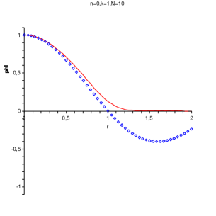
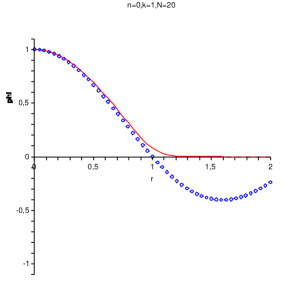
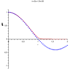
Figure 2: Comparison of the radial shape for the symbol $\Phi^{\left(N\right)}_{0,1}\left(r,\varphi\right)$ (continuum line), the symbol of the eigenmatrix of the fuzzy Laplacian for $N=10,20,30$, with $\Phi_{0,1}\left(r,\varphi\right)$.

This behaviour is seen to be valid also for eigenstates of different eigenvalues. The plots for the symbols $\Phi_{0,2}^{\left(N\right)}$ are in figure 3, those for $\Phi_{0,3}^{\left(N\right)}$ in figure 4.

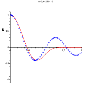
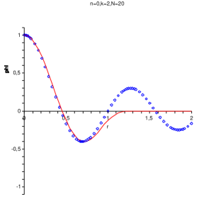
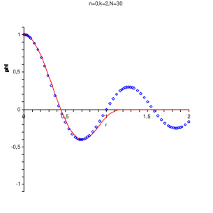
Figure 3: Comparison of the radial shape for the symbol $\Phi_{0,2}^{\left(N\right)}\left(r\right)$ (continuum line) with $\Phi_{0,2}\left(r\right)$ for $N=10,20,30$.

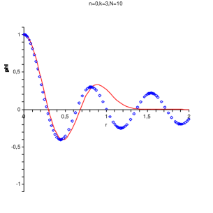
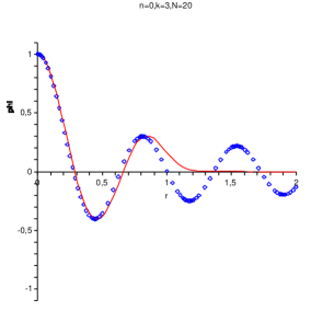
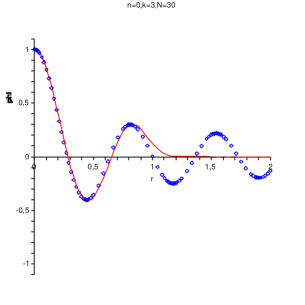
Figure 4: Comparison of the radial shape for the symbol $\Phi_{0,3}^{\left(N\right)}\left(r\right)$ (continuum line) with $\Phi_{0,3}\left(r\right)$ for $N=10,20,30$.

It is interesting to analyse the fuzzification of $\Phi_{0,10}\left(r\right)$. The fuzzy symbol is $\hat{\Phi}_{0,10}^{\left(N\right)}$. For $N=10,20,25$ it is plotted in figure (5).

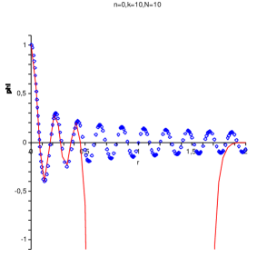
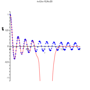
Figure 5: Comparison of the radial shape for the $\Phi_{0,10}^{\left(N\right)}$ symbol (continuum line)for $N=10,20,25$. The bump goes out of the picture. As $N$ increases, it becomes narrower and narrower.

It is evident that the fuzzy eigenfunction reproduces the continuum eigenfunction for values of $r$ close to the centre of the disc, but not on the edge, where a huge bump appears. In [15] it has been explained that the presence of the bump on the edge of the disc, in the fuzzification of a function defined on the plane, is related to the fact that this function has oscillations of too small wavelenght compared to $\theta$. This is manifestation of the infrared-ultraviolet mixing characteristic of noncommutative theories. In the case of $\Phi_{0,10}\left(r\right)=J_{0}\left(\sqrt{\lambda_{0,10}}r\right)$, one can immediately see that the oscillation wavelenght of the continuum eigenfunction is given by $\rho_{\lambda}\,\sim\,1/k\,\sim 1/10$. In these plots, it is assumed $\theta=1/N$ (the fuzzy disc truncation), so $\theta$ and $\rho_{\lambda}$ are of compatible magnitude. In the fuzzy disc limit, $N\,\rightarrow\,\infty$, so $\theta$ is infinitesimal. The bump disappears, as it is shown in the other plots (figure 6).

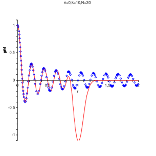
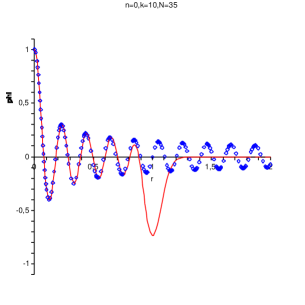
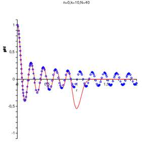
Figure 6: Comparison of the radial shape for the $\Phi_{0,10}^{\left(N\right)}$ symbol for $N=30,35,40$.

The non radial functions follow a similar pattern. Their phases are exactly as the ones of their continuum counterparts, while the radial parts are similar. A first plot is in Fig. 7, a second one in Fig. 8, where the fuzzification procedure gives again a bump, for small values of $N$. This bump is seen to disappear in the fuzzy disc limit.

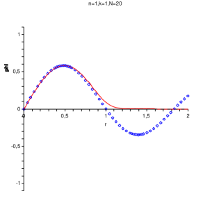
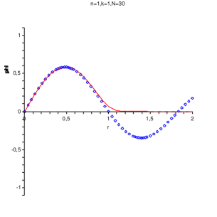
Figure 7: Comparison of the radial shape of the $\Phi_{1,1}^{\left(N\right)}\left(r,\varphi\right)$ symbol (continuum line) for $N=10,20,30$.

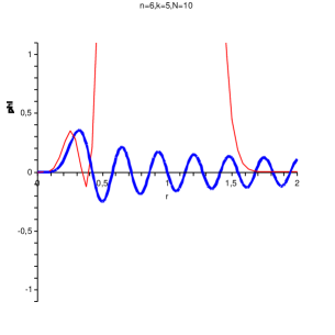
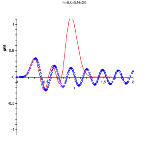
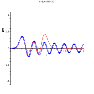
Figure 8: Comparison of the radial shape of the $\Phi_{6,5}^{\left(N\right)}\left(r,\varphi\right)$ symbol (continuum line) for $N=10,20,30$.

The fuzzy Bessels, being eigenfunctions, provide an efficient way to calculate a fuzzy Green function, which we calculated numerically in [15]. Since the fuzzy Laplacian is represented by an hermitian finite dimensional matrix, its inverse can be written in terms of a spectral decomposition. If a matrix, say $M$, is hermitian, then its components satisfy the condition $M_{ab}=M_{ba}^{*}$ in terms of transposition and complex conjugation. The eigenvalue problem gives a number of real eigenvalues equal to the dimension of the space on which the matrix acts:

$$\sum_{b}M_{ab}v_{b}^{\left(k\right)}=\lambda^{\left(k\right)}v_{a}^{\left(k\right)}\ ,$$ (4.66)

here $v_{a}^{\left(k\right)}$ indicates the $a^{th}$ components of the eigenvector relative to the eigenvalue $\lambda^{\left(k\right)}$. The inverse, if it exists, of the matrix $M$ is a matrix $G$ whose components can be written as:

$$G_{sq}=\sum_{k}\,v_{s}^{\left(k\right)}v_{q}^{\left(k\right)}/\lambda^{\left(k\right)}\ .$$ (4.67)

If we specialise to the problem under analysis, the notion of eigenvector of components $v_{a}^{\left(N\right)}$ with eigenvalue $\lambda^{\left(k\right)}$ goes into that of fuzzy Bessel $\hat{\Phi}^{\left(N\right)}_{n,k}$ matrix, from which it is immediate to obtain the symbols. The fuzzy Green function becomes:

$$G^{\left(N\right)}_{\theta}\left(z,z^{\prime}\right)=\sum_{n=-N}^{+N}\sum_{k=1}^{N+1-\left|n\right|}\frac{\Phi_{n,k}^{\left(N\right)}\left(z^{\prime}\right)^{*}\Phi_{n,k}^{\left(N\right)}\left(z\right)}{\lambda^{\left(N\right)}_{|n|,k}}\ .$$ (4.68)

Since the fuzzy Bessels play a role similar to fuzzy harmonics for the fuzzy sphere algebra, we can now make describe the process of approximating the algebra of functions on a disc with matrices more precise. In complete analogy with (2.18) and (2.19), if $f$ is square integrable with respect to the standard measure on the disc $d\Omega=rdrd\phi$, it can be expanded in terms of Bessel functions:

$$f\left(r,\varphi\right)=\sum_{n=-\infty}^{+\infty}\,\sum_{k=1}^{\infty}\,f_{nk}e^{in\varphi}J_{\left|n\right|}\left(\sqrt{\lambda_{\left|n\right|,k}}r\right)$$ (4.69)

and it is possible to truncate:

$$f^{\left(N\right)}\left(r,\varphi\right)=\sum_{n=-N}^{+N}\sum_{k=1}^{N+1-|n|}\,f_{nk}e^{in\varphi}J_{\left|n\right|}\left(\sqrt{\lambda_{\left|n\right|,k}}r\right)=\sum_{n=-N}^{+N}\sum_{k=1}^{N+1-|n|}\,f_{nk}\,\Phi_{n,k}\left(r,\varphi\right)\ .$$ (4.70)

This set of functions is a vector space, but it is no more an algebra, with the standard definition of sum and pointwise product, as the product of two truncated functions will get out of the algebra. The mapping from truncated functions into finite rank matrices:

$$f^{(N)}\rightarrow\hat{f}^{\left(N\right)}_{\theta}=\sum_{n=-N}^{+N}\sum_{k=1}^{N+1-|n|}\,f_{nk}\hat{\Phi}_{n,k}^{\left(N\right)}$$ (4.71)

endows the set of functions with a noncommutative product, inherited from the matrix product, which makes it into a non abelian algebra. The formal limit $N\rightarrow\infty$ with the constraint $N\theta=1$ is the abelian algebra of functions on the disc. The sequence of nonabelian algebras $\mathcal{A}_{\theta}^{(N)}$ is what we call the fuzzy disc.

A Weyl-Wigner Formalism

In this appendix we give a very short introduction to the Weyl-Wigner formalism used to define maps between functions on a “classical” plane and a set of operators on a Hilbert space [24].

Given a symplectic real, finite dimensional, vector space $\left(L,\omega\right)$, where the symplectic form $\omega$ is translationally invariant, i.e. with constant coefficients, the set of Displacement operators define a Weyl system, a unitary representation of canonical commutation relations in the exponentiated unitary version [33]:

$$\hat{D}\, : \,L\,\mapsto\,\mathcal{U}\left(\mathcal{H}\right)$$

$$\hat{D}\left(z+u\right) = e^{i\omega\left(z,u\right)/2\theta}\hat{D}\left(z\right)\hat{D}\left(u\right)\ .$$ (A.1)

Here $\theta$ is a parameter: the Displacement operators can be seen to set a unitary projective representation of the translation group, where the phase factor is related to the sympletic structure defined on the vector space $L$. These operators also define a representation of the Heisenberg-Weyl group [34]. On every one dimensional subspace of $L$ ($\alpha$ is a real scalar), via the Stone-von Neumann theorem:

$$\hat{D}\left(\alpha z\right)=e^{i\alpha\hat{G}\left(z\right)\theta}$$ (A.2)

and these generators satisfy:

$$\left[\hat{G}\left(z\right),\hat{G}\left(u\right)\right]\,=\,i\theta\omega\left(z,u\right)\,{1\!\!1}\ .$$ (A.3)

This shows that a Weyl system is a way to formalise a set of canonical commutation relations for quantum observables, recovered as hermitian generators of a unitary ray representation. In this perspective $\theta$ acquires the role of a noncommutativity parameter. In the standard approach, the symplectic vector space is seen as a phase space for the classical dynamics of point particle: generators of a Weyl system represent the position and momentum observable for a quantum dynamics of point particle.

Using the definition of a Weyl system, it is possible to define a Weyl map, that is a map from functions on the vector space $\left(L\omega\right)$ (dim $L=2n$) to $Op\left(\mathcal{H}\right)$, the set of operators on the Hilbert space on which Displacements are realised:

$$\hat{f}=\int\,\frac{dw}{\left(2\pi\theta\right)^{n}}\,\tilde{f}\left(w\right)\hat{D}\left(w\right)\ ,$$ (A.4)

where:

$$\tilde{f}\left(w\right)=\int\frac{dz}{\left(2\pi\theta\right)^{n}}\,f\left(z\right)\,e^{-i\omega\left(z,w\right)/\theta}$$ (A.5)

is the symplectic Fourier transform [34] of the function $f$. The Weyl map can be seen as a quantization map for classical observables defined on a phase space: it can be inverted by the Wigner map:

$$\tilde{f}\left(w\right)=Tr\left[\hat{f}\hat{D}^{\dagger}\left(w\right)\right]\ .$$ (A.6)

So the Weyl-Wigner maps define a bijection between a set of classical observables and a set of quantum observables. This is the building block of a formalism suited to study both the problem of quantizing a classical system and performing a classical limit of a quantum system.

The standard Weyl-Wigner maps can be modified by the introduction of a term, called weight:

$$\hat{f}_{\lambda}\, = \,\int\,\frac{dw}{\left(2\pi\theta\right)^{n}}\,\tilde{f}\left(w\right)\lambda\left(w\right)\hat{D}\left(w\right)$$

$$\tilde{f}\left(w\right) = \lambda\left(w\right)^{-1}Tr\left[\hat{f}_{\lambda}\hat{D}^{\dagger}\left(w\right)\right]\ .$$ (A.7)

This weight can be proved to be related to a more general class of ray representation of the translation group, and is seen to be responsible both for a specific ”ordering” in the quantization procedure and a definition of a specific domain of mathematical applicability of the bijection, as stressed in the main text.

B Generalised coherent states

In this paper the concept of generalised coherent states has been extensively used. The aim of this appendix is to briefly recollect the main definitions and results, to fix notations and facilitate the reading. The main reference for coherent states is [35].

Consider a Lie group $G$, and $\hat{U}\left(g\right)$ a unitary irreducible representation of this group on a Hilbert space $\mathcal{H}$. Chosen a fiducial vector $|\psi_{0}\rangle$ in $\mathcal{H}$, one obtains a set of vectors for each element of the group, acting on it with $\hat{U}\left(g\right)$:

$$|\psi_{g}\rangle\,\equiv\,\hat{U}\left(g\right)|\psi_{0}\rangle\ .$$ (B.1)

Two such vectors are considered equivalent if they correspond, quantum-mechanically, to the same state, i.e. if they differ by a phase. So $|\psi_{g}\rangle\,\simeq\,|\psi_{g^{\prime}}\rangle$ if $|\psi_{g}\rangle\,=e^{i\phi\left(g,g^{\prime}\right)}\,|\psi_{g^{\prime}}\rangle$. This condition is equivalent to $\hat{U}\left(g^{\prime-1}g\right)|\psi_{0}\rangle\,=e^{i\phi\left(g,g^{\prime}\right)}\,|\psi_{0}\rangle$. If $H$ is the subgroup of $G$ whose elements are represented, by $\hat{U}$, as operators whose action on the fiducial vector is just a multiplication by a phase, then the equivalence relation is among points of $G$, and the quotient is the space $G/H$. If $H$ is maximal, then it is called isotropy subgroup for the state $|\psi_{0}\rangle$. Choosing a representative $g\left(x\right)$ in each equivalence class $x\,\in\,X=G/H$ (which is a cross section of the fiber bundle $G$ with base $X$) defines a set of vectors on $\mathcal{H}$, depending, clearly, on $G$ and $|\psi_{0}\rangle$. This set of states is called a system of coherent states for $G$. The state corresponding to the vector $|x\rangle$ may be considered as the range of a rank one projector in $\mathcal{H}$. Thus, the system of generalised coherent states determines a set of one dimensional subspaces in $\mathcal{H}$, parametrised by points of the homogeneous space $X=G/H$. An evolution of this analysis drives naturally to the issue of overcompleteness for the system of coherent states, mentioned in (3.34), (2.6).

C Explicit Calculations for the Eigenvalues

The aim of this appendix is to show an explicit proof of the results claimed in the main text about the eigenvalue problem for the fuzzy Laplacian. In particular, we want to prove that the equation (4.57) is equivalent to the equation (4.60). From this equivalence, it will be proved also the equivalence between equations (4.43) and equation (4.47), as they are a special case of the first two for $n=0$.

The polynomial $E_{N}^{\left(n\right)}$ is given, identifying $\lambda^{\left(N\right)}_{n,k}/4N=x^{N}$, by (4.50):

$$E_{N}^{\left(n\right)}\left(x_{N}\right)=\sum_{k=0}^{N-n+1}\,\left(-1\right)^{k+N-n+1}\,\frac{\left(N+1\right)!\left(N-n+1\right)!}{k!\left(n+k\right)!\left(N-n-k+1\right)!}\,\left(x_{N}\right)^{k}=0\ .$$ (C.2)

The characteristic polynomial $P^{\left(n\right)}_{N}$ is given by the determinant of the matrix (4.58) given recursively by (4.59). To prove the equality of the two polynomials, the first step is to prove that $E_{N}^{\left(n\right)}$ satisfies the same recursive relation that $P_{N}^{\left(n\right)}$ does.

Considering the quantity:

$$\left(x_{N}-\left(2N-n+1\right)\right)\,E_{N-1}^{\left(n\right)}\left(x_{N}\right)\,-\,N\left(N-n\right)\,E_{N-2}^{\left(n\right)}\left(x_{N}\right)=$$

$$=\sum_{k=0}^{N-n}\left(-1\right)^{k+N-n}\frac{N!\left(N-n\right)!}{k!\left(n+k\right)!\left(N-n-k\right)!}\,\left(x_{N}\right)^{k+1}\,+$$

$$-\sum_{k=0}^{N-n}\left(-1\right)^{k+N-n}\left(2N-n+1\right)\frac{N!\left(N-n\right)!}{k!\left(n+k\right)!\left(N-n-k\right)!}\,\left(x_{N}\right)^{k}\,+$$

$$-\sum_{k=0}^{N-n-1}\left(-1\right)^{k+N-n+1}\frac{N!\left(N-n\right)!}{k!\left(n+k\right)!\left(N-n-k-1\right)!}\,\left(x_{N}\right)^{k}\ .$$ (C.3)

Where the coefficient of the zeroth order term is:

$$\left(\left(-1\right)^{N-n+1}\frac{N!}{n!}\left(2N-n+1\right)-\left(-1\right)^{N-n+1}\frac{N!}{n!}\left(N-n\right)\right)=\left(-1\right)^{N-n+1}\frac{\left(N+1\right)!}{n!}\ .$$ (C.4)

It coincides with the coefficient of the zeroth order term of the polynomial $E^{\left(n\right)}_{N}$.

Let us consider, in the expression (C.3), the coefficient of the $q^{th}$ order term, with $1\leq q\leq N-n-1$. It is equal to:

$$\left(-1\right)^{N-n+q-1}N!\left(N-n\right)!\left(\frac{1}{\left(a-1\right)!\left(n+a-1\right)!\left(N-n-a+1\right)!}+\right.$$

$$\left.\frac{2N-n+1}{a!\left(n+a\right)!\left(N-n-a\right)!}-\frac{1}{a!\left(n+a\right)!\left(N-n-a-1\right)!}\right)\left(x_{N}\right)^{q}=\left(-1\right)^{N-n+a+1}\frac{\left(N+1\right)!\left(N-n+1\right)!}{a!\left(a+n\right)!\left(N-n-a+1\right)!}\left(x_{N}\right)^{q} \ .$$

This coefficient is equal to the coefficient of the $q^{th}$ order term in $E_{N}^{\left(n\right)}$. The equality of the coefficients, of the remaining order terms, of the polynomial (C.3) with those of the polynomial $E^{\left(n\right)}_{N}\left(x_{N}\right)$ can be easily checked.

At this stage, we have proved that the polynomial $E^{\left(n\right)}_{N}\left(x_{N}\right)$ satisfies the same recursive relation that the polynomial $P^{\left(n\right)}_{N}\left(x_{N}\right)$ does satisfy. The recursive relation they satisfy is such that the $N^{th}$ term of the sequence $E_{N}^{\left(n\right)}$, for each fixed $n$, depends on both the $\left(N-1\right)^{th}$ and $\left(N-2\right)^{th}$ terms of the sequence. To prove the complete equivalence of these two polynomials, we thus need to prove that they explicitly coincide at a pair of consecutive steps.

In the main text it has been stressed that there is a constraint for allowed positive $n$, namely an upper bound: $n\,\leq\,N+1$. This means that, for a fixed $n$, that is for a fixed subspace in the fuzzy algebra, $N\,\geq\,n+1$. For $N=n-1$ both polynomials $E_{n-1}^{\left(n\right)}\left(x_{N}\right)$ and $P_{n-1}^{\left(n\right)}\left(x_{N}\right)$ are trivial, so we study at first the case of $N=n$. We have:

$$E_{n}^{\left(n\right)}=\sum_{k=0}^{1}\,\left(-1\right)^{k+1}\,\frac{\left(n+1\right)!}{k!\left(n+k\right)!\left(1-k\right)!}\,\left(x^{\left(N\right)}\right)^{k}=x^{\left(N\right)}-\left(n+1\right)$$ (C.6)

while the matrix representing the action of the fuzzy Laplacian is one-dimensional, so that:

$$P_{n}^{\left(N\right)}=x_{N}-\left(2n+1\right)\ .$$ (C.7)

The second case is for $N=n+1$. We have:

$$E_{n}^{\left(n+1\right)} = \sum_{k=0}^{2}\,\left(-1\right)^{k+2}\,\frac{2\left(n+2\right)!}{k!\left(n+k\right)!\left(2-k\right)!}\,\left(x_{N}\right)^{k}$$ (C.8)

$$= \,\left(x_{N}\right)^{2}-2\left(n+2\right)x_{N}+\left(n+1\right)\left(n+2\right)\ .$$

The matrix representing the action of the fuzzy Laplacian is now two-dimensional, so that the characteristic polynomial is:

$$P_{n+1}^{\left(n\right)} = \det\left(\begin{array}[]{cc}x_{N}-\left(n+1\right)&\sqrt{n+1}\\ \sqrt{n+1}&x_{N}-\left(n+3\right)\end{array}\right)\,=$$ (C.11)

$$= \left(x_{N}\right)^{2}-2\left(n+2\right)x_{N}+\left(n+1\right)\left(n+2\right)\ .$$ (C.12)

This proves the equivalence of the two polynomials.

Acknowledgments

We thank D. Bercioux, P. Lucignano, P. Santorelli and A. Stern for help at various stages. This work has been supported in part by the Progetto di Ricerca di Interesse Nazionale SInteSi.

References

- [1]
- [2] A. Connes, Noncommutative Geometry, Academic Press (1994).
- [3] G. Landi, An introduction to Noncommutative Spaces and their Geometries, vol.51 of Lecture Notes in Physics. New Series M, Monographs (1997), hep-th/9701078.
- [4] J.M. Gracia-Bondìa, J.C. Várilly, H.Figueroa, Elements of Noncommutative Geometry, Birkhäuser (2000).
- [5] J.Madore, An introduction to noncommutative differential geometry and its physical applications, Lect.Notes London Math.Soc. 206 (1995) Cambridge University Press.
- [6] J. Madore, “The fuzzy sphere”, Class. Quant. Grav. 9, 69 (1992).
- [7] M. Rieffel, “ Metrics on state spaces”, math.OA/9906151; “Matrix algebras converge to the sphere for quantum Gromov-Hausdorff distance”, math.OA/0108005; “Gromov-Hausdorff distance for quantum metric spaces”, math.OA/0011063.
- [8] C. S. Chu, J. Madore and H. Steinacker, “Scaling limits of the fuzzy sphere at one loop”, JHEP 0108 (2001) 038, hep-th/0106205.
- [9] S. Ramgoolam, “On spherical harmonics for fuzzy spheres in diverse dimensions”, Nucl. Phys. B 610, 461 (2001), hep-th/0105006.
- [10] H. Grosse, C. Klimcik and P. Presnajder, “Towards finite quantum field theory in noncommutative geometry”, Int. J. Theor. Phys. 35, 231 (1996), hep-th/9505175; U. Carow-Watamura and S. Watamura, “Noncommutative geometry and gauge theory on fuzzy sphere”, Commun. Math. Phys. 212, 395 (2000), hep-th/9801195; A. P. Balachandran, X. Martin and D. O’Connor, “Fuzzy actions and their continuum limits”, Int. J. Mod. Phys. A 16, 2577 (2001), hep-th/0007030; S. Iso, Y. Kimura, K. Tanaka and K. Wakatsuki, “Noncommutative gauge theory on fuzzy sphere from matrix model”, Nucl. Phys. B 604, 121 (2001), hep-th/0101102; Y. Kimura, “Noncommutative gauge theories on fuzzy sphere and fuzzy torus from matrix model”, Prog. Theor. Phys. 106, 445 (2001), hep-th/0103192; A. Y. Alekseev, S. Fredenhagen, T. Quella and V. Schomerus, “Non-commutative gauge theory of twisted D-branes”, Nucl. Phys. B 646, 127 (2002), hep-th/0205123; H. Steinacker, “Quantized gauge theory on the fuzzy sphere as random matrix model”, Nucl. Phys. B 679, 66 (2004), hep-th/0307075; S. Vaidya and B. Ydri, “On the origin of the UV-IR mixing in noncommutative matrix geometry”, Nucl. Phys. B 671, 401 (2003), hep-th/0305201; A. Pinzul and A. Stern, “A perturbative approach to fuzzifying field theories”, hep-th/0502018.
- [11] Y. Kimura, “Noncommutative gauge theory on fuzzy four-sphere and matrix model”, Nucl. Phys. B 637, 177 (2002), hep-th/0204256; J. Medina and D. O’Connor, “Scalar field theory on fuzzy S(4)”, JHEP 0311, 051 (2003), hep-th/0212170.
- [12] M. Rieffel, ”-algebras associated with irrational rotations”, Pacific J. Math. 93 (1981) 415; “Noncommutative Tori - a case study of noncommutative differentiable manifold”, Contemp. Math. 105 (1990) 191.
- [13] F. Lizzi, “Fuzzy two-dimensional spaces”, Proceedings to the Euroconference Beyond the standard model, Portoroz, 2003, N. Mankoc Borstnik, H.B Nielsen, C.D. Froggatt, D. Lukman Eds., hep-ph/0401043.
- [14] H. Grosse and A. Strohmaier, “Noncommutative geometry and the regularization problem of 4D quantum field theory”, Lett. Math. Phys. 48 (1999) 163, hep-th/9902138; G. Alexanian, A. P. Balachandran, G. Immirzi and B. Ydri, “Fuzzy CP(2)”, J. Geom. Phys. 42 (2002) 28, hep-th/0103023; A. P. Balachandran, B. P. Dolan, J. H. Lee, X. Martin and D. O’Connor, “Fuzzy complex projective spaces and their star-products”, J. Geom. Phys. 43 (2002) 184, hep-th/0107099; S. Vaidya, “Perturbative dynamics on fuzzy S(2) and RP(2)”, Phys. Lett. B 512, 403 (2001), hep-th/0102212.
- [15] F. Lizzi, P. Vitale and A. Zampini, “The fuzzy disc”, JHEP 0308, 057 (2003), hep-th/0306247.
- [16] F. Lizzi, P. Vitale and A. Zampini, “From the fuzzy disc to edge currents in Chern-Simons theory”, Mod. Phys. Lett. A 18, 2381 (2003), hep-th/0309128.
- [17] A. P. Balachandran, K. S. Gupta and S. Kurkcuoglu, “Edge currents in non-commutative Chern-Simons theory from a new matrix model”, JHEP 0309, 007 (2003), hep-th/0306255.
- [18] A. Pinzul and A. Stern, “Edge states from defects on the noncommutative plane”, Mod. Phys. Lett. A 18, 2509 (2003), hep-th/0307234.
- [19] F. A. Berezin, “General Concept Of Quantization”, Commun. Math. Phys. 40, 153 (1975).
- [20] H. Figueroa, J.M. Gracia-Bondía, J.C. Vá rilly, “Moyal quantization with compact symmetry groups and noncommutative harmonic analysis”, J. Math. Phys. 31 11 (1990) 2664.
- [21] H. Grosse and P. Presnajder, “The Construction on noncommutative manifolds using coherent states”, Lett. Math. Phys. 28 (1993) 239.
- [22] A. Zampini, Applications of the Weyl-Wigner formalism to noncommutative geometry, PhD thesis, University of Naples, January 2005. hep-th/0505271.
- [23] D.A.Varshalovich, A.N.Moskalev, V.K.Kersonskii, Quantum Theory of Angular Momentum, World Scientific (1988).
- [24] M. Hillery, R. F. O’Connell, M. O. Scully and E. P. Wigner, “Distribution Functions In Physics: Fundamentals”, Phys. Rept. 106, 121 (1984).
- [25] A. Voros, “Wentzel-Kramers-Brillouin method in the Bargmann representation”, Phys. Rev. A 40 (1989) 6814.
- [26] G. Alexanian, A. Pinzul and A. Stern, “Generalized Coherent State Approach to Star Products and Applications to the Fuzzy Sphere”, Nucl. Phys. B 600, 531 (2001), hep-th/0010187.
- [27] H.J. Groenewold, “On the Principles of Elementary Quantum Mechanics”, Physica 12 (1946) 405.
- [28] J.E. Moyal, “Quantum Mechanics as a Statistical Theory”, Proc. Cambridge Phil. Soc. 45 (1949) 99.
- [29] V. Gayral, J. M. Gracia-Bondia, B. Iochum, T. Schucker and J. C. Varilly, “Moyal planes are spectral triples”, Commun. Math. Phys. 246 (2004) 569, hep-th/0307241.
- [30] A.P. Prudnikov, Y.A. Brychkov, O.I. Marichev, Integrals and Series, Gordon and Breach Science Publishers (1988).
- [31] V.I. Smirnov, A course of higher mathematics I.N. Sneddon ed., Pergamon Press, 1964.
- [32] F.R. Gantmacher, Applications of the theory of matrices, Interscience (1959).
- [33] J.C. Baez, I.E. Segal, Z. Zhou, Introduction to Algebraic and Constructive Quantum Field Theory, Princeton Univ. Press (1992).
- [34] G.B. Folland, Harmonic Analysis in Phase Space, Princeton University Press (1989).
- [35] A. Perelomov, Generalized Coeherent States and Their Applications, Springer-Verlag (1986).