More about spontaneous Lorentz-violation and infrared modification of gravity

Abstract:

We consider a model with Lorentz-violating vector field condensates, in which dispersion laws of all perturbations, including tensor modes, undergo non-trivial modification in the infrared. The model is free of ghosts and tachyons at high 3-momenta. At low 3-momenta there are ghosts, and at even lower 3-momenta there exist tachyons. Still, with appropriate choice of parameters, the model is phenomenologically acceptable. Beyond a certain large distance scale and even larger time scale, the gravity of a static source changes from that of General Relativity to that of van Dam–Veltman–Zakharov limit of the Fierz–Pauli theory. Yet the late time cosmological evolution is always determined by the standard Friedmann equation, modulo small correction to the “cosmological Planck mass”, so the modification of gravity cannot by itself explain the accelerated expansion of the Universe. The latter property is generic in a wide class of models with condensates.

1 Introduction and summary

Recently, there have been several attempts to construct theories in which gravity gets modified at ultra-large distance and time scales [1, 2, 3, 4, 5, 6, 7] (see also Ref. [8] and references therein). One of the motivations is to explain the accelerated expansion of the Universe by a modification of the Friedmann equation rather than by introducing the cosmological constant or exotic matter such as quintessence. Most of the Lorentz-invariant models with unconventional gravity in the infrared either have ghosts or suffer from the strong coupling problem at unacceptably low energies [9] (see, however, Ref. [10]). These problems need not be inherent in Lorentz-violating theories [3, 5, 11, 6], so it is natural to study possible infrared modifications of gravity in the context of Lorentz-violation. In this paper we consider one model of this sort, to see what kinds of features may emerge once Lorentz-invariance gets broken.

One way to introduce spontaneous Lorentz-violation is to invoke condensates of vector (or, more generally, tensor) fields [12, 13, 14, 15, 16, 11, 17, 18]. Requiring symmetry under spatial rotations, one can either consider a condensate of the time component $B_{0}$ of a vector field $B_{\mu}$ [12, 13, 14], or introduce internal global symmetry $G$ and allow for condensates of spatial components which break $G\times SO(3)_{S}$ but leave unbroken an $SO(3)$ subgroup, where $SO(3)_{S}$ is the original group of spatial rotations. The simplest version of the latter construction (cf. Ref. [19]) involves three vector fields $A_{\mu}^{a}$, $a=1,2,3$, a triplet under $G\equiv SO(3)_{G}$, whose condensates are

$$A_{i}^{a}=\mu\delta_{i}^{a}$$ (1)

where $i=1,2,3$ is the spatial index. Of course, both types of condensates, $B_{0}$ and $A_{i}^{a}$, may be present in one and the same model, and in this paper we consider precisely the latter possibility.

Vector fields condense if their Lagrangian contains a potential term $V(B_{\mu},A_{\mu}^{a})$. Hence, the theory of vector fields is definitely not gauge-invariant. In this case the kinetic terms in the vector field Lagrangian are generally not gauge-invariant as well. Without gauge invariance, there is a danger of ghosts whose 3-momenta could be unacceptably high. However, this is not necessarily the case in the presence of vector field condensates [11]. In this paper we make use of the mechanism of Ref. [11] to avoid ghosts at high momenta.

Violation of Lorentz-invariance by vector field condensates generically leads to new light modes which are mixtures of gravitational and vector field excitations. In models considered so far, the dispersion laws for these modes, as well as for transverse-traceless descendants of gravitons, is $\omega^{2}\propto k^{2}$, with propagation velocities generally different for different modes. This possibility has been extensively studied in literature, and, indeed, it has a number of interesting phenomenological consequences [20, 21]. We note, however, that in these models, no modification of the dispersion laws occur at ultra-low spatial momenta. This is in contrast to the Higgs mechanism in gauge theories. Unlike in gauge theories, the Lorentz connections are proportional to derivatives of the fundamental field, the metric. Hence, the terms in the vector field Lagrangian, quadratic in covariant derivatives, upon condensation lead to two-derivative terms in the Lagrangian for the metric perturbations; symbolically

$$DA\cdot DA\to\mu^{2}(\Gamma\cdot\Gamma)\propto\mu^{2}\cdot\partial h\partial h$$

where $\Gamma_{\nu\lambda}^{\mu}$ are Christoffel symbols, and $h_{\mu\nu}$ are metric perturbations about Minkowski background. On the other hand, because of general covariance, the potential $V(B,A)$ does not generate a mass for the graviton, although it may generate mixing between the graviton and vector field perturbations about their condensates. Hence, if the vector Lagrangian contains terms with zero and two derivatives only, the dispersion relation for the graviton (possibly with admixture of vector fields) is, at low 3-momenta $k$,

$$\omega^{2}=\mathrm{v}^{2}\cdot k^{2}$$ (2)

where

$$\mathrm{v}=1+O\left(\frac{\mu^{2}}{M_{Pl}^{2}}\right)$$

Unlike in gauge theories with the Higgs mechanism, the disperison law (2) is valid at arbitrarily low spatial momenta.

In this paper we explore a possibility that, besides the potential term $V(B,A)$ and kinetic two-derivative terms, the vector field Lagrangian contains terms with one derivative, e.g.,

$$\lambda\varepsilon_{abc}\cdot D_{\mu}A_{\nu}^{a}A^{b\mu}A^{c\nu}$$ (3)

where $\lambda\ll 1$. We assume that except for $\lambda$, the vector field Lagrangian does not contain very small dimensionless parameters, and that $\mu\ll M_{Pl}$. Upon vector field condensation (1), the term (3) becomes an addition to the quadratic Lagrangian for perturbations of the vector fields and metric, which is linear in derivatives and is characterized by the scale $\lambda\mu$. Even without gravity, introducing the term (3) brings in a new feature: there reappear ghosts, but only at low 3-momenta, $p\lesssim\lambda\mu$. Unlike in Lorentz-invariant theories, these ghosts — negative energy excitations — are not unacceptable provided that $\lambda\mu$ is low enough [22, 6] (see also Ref. [23]); they may even be useful in the cosmological context [24]. In a certain window of 3-momenta around $p\sim\lambda\mu$, there may also appear tachyons, which are by far more dangerous. In the model we consider, tachyons are absent at the expense of fine-tuning of the parameters.

Another effect of the term (3) in the theory without gravity is that at $k\ll\lambda\mu$, one of the modes (a 3-scalar) has the dispersion relation

$$\omega^{2}\propto k^{4},\ \ \ \ k\ll\lambda\mu$$ (4)

i.e. it behaves like an excitation of ghost condensate [3].

With gravity turned on, two other, even lower scales appear. One of them is

$$\Lambda_{(1)}=\lambda\mu\cdot\frac{\mu}{M_{Pl}}$$ (5)

This scale determines the distance at which the gravitational field of a static source gets modified: at $r\ll\Lambda_{(1)}^{-1}$ this field is the same as in General Relativity, while at $r\gg\Lambda_{(1)}^{-1}$ it has the (scalar-tensor) form of the van Dam–Veltman–Zakharov limit of the Fierz–Pauli theory,

$$r\ll\Lambda_{(1)}^{-1}:\mbox{ GR}\ \ \longrightarrow\ \ \ r\gg\Lambda_{(1)}^{-1}:\mbox{ FP}$$ (6)

Also, at this scale the dispersion relation for the “ghost-condensate-like” mode changes from (4) back to $\omega^{2}\propto k^{2}$,

$$k\gg\Lambda_{(1)}:\ \ \omega^{2}\propto k^{4}\ \ \longrightarrow\ \ \ k\ll\Lambda_{(1)}:\ \ \omega^{2}\propto k^{2}$$

In fact, it is this mode that adds to the gravitational interaction between the static sources at $r\gg\Lambda_{(1)}^{-1}$.

The lowest scale that appears in our model is

$$\Lambda_{(2)}=\lambda\mu\frac{\mu^{2}}{M_{Pl}^{2}}$$

At this scale the behavior of 3-tensor and 3-vector modes changes considerably. While at $k\gg\Lambda_{(2)}$ the dispersion laws in these sectors have the form (2), at low 3-momenta $(k\ll\Lambda_{(2)})$ there exist modes with the dispersion law

$$\omega^{2}\propto\pm k$$

In particular, there are tachyons in the spectrum. They are not unacceptable, provided that $\Lambda_{(2)}$ is small enough, say, $\Lambda_{(2)}\lesssim H_{0}$, where $H_{0}$ is the present value of the Hubble parameter. Furthermore, at the very first sight, tachyons are a welcome feature from the cosmological viewpoint: gravity becomes unstable at very large distances and times.

Roughly the same scale determines the time at which gravitational field of a static source gets modified from GR to FP. The separation between this time scale and the distance scale, Eq. (5), is basically the same phenomenon as the one found in the ghost condensate model [3]. In fact, the time scale relevant to the modification of Newton’s law may be smaller than $\Lambda_{(2)}^{-1}$. We will keep track of one of the parameters of our model, call it $\alpha^{B}$, and see that the time scale is actually

$$\frac{1}{\sqrt{\alpha^{B}}\Lambda_{(2)}}$$

Thus, gravity of static sources may get modified well before the space becomes unstable.

We will see, however, that in spite of all these peculiarities, the Friedmann equation governing the evolution of spatially flat, homogeneous and isotropic Universe remains precisely the same as in GR, provided that the vector fields have settled down to their condensate values (there are light modes that can in principle serve as unusual particles filling the Universe; we will not consider this possibility in the present paper). The only difference with respect to GR is that the “cosmological Newton’s constant” is not exactly equal to the gravitational constant entering Newton’s law at $r\ll\Lambda_{(2)}^{-1}$ — the phenomenon found in Refs. [16, 17]. Thus, condensation of vector fields cannot by itself explain the accelerated expansion of the Universe. Furthermore, we will argue (see also Ref. [18]) that in four-dimensional local theories allowing for derivative expansion, the form of the gravitational side of the Friedmann equation for spatially flat Universe, $H^{2}$, is fixed by symmetries, so it is unlikely that the accelerated expansion would occur in four-dimensional theories solely due to the condensation of any tensor fields. In this regard, brane world scenarios with infinite extra dimensions appear more promising.

We are not going to discuss phenomenology of our model in this paper. We only note that for sufficiently small $\mu$ and very small $\lambda\mu$, this model should be phenomenologically acceptable, and that the constraints obtained, e.g., in Refs. [17, 20, 21, 22] should apply, with appropriate modifications, to our model as well. The model displays a number of potentially interesting features — ghosts at low 3-momenta, tachyons at even lower 3-momenta, modification of the gravitational fields of sources at large times and not so large distances. It remains to be understood whether these features may be phenomenologically useful.

2 The model

We consider a generally covariant theory with vector fields $B_{\mu}$ and $A_{\mu}^{a}$. The latter form a triplet under global symmetry group $SO(3)_{G}$. We take the action in the form

$$S=\int\limits\!d^{4}x\sqrt{-g}\left(\mathcal{L}_{EH}+\mathcal{L}_{V}^{(2)}+\mathcal{L}_{V}^{(1)}-V\right)$$ (7)

where [signature $(+,-,-,-,)$]

$$\mathcal{L}_{EH}=-M_{Pl}^{2}R$$

is the Einstein-Hilbert term, and the terms $\mathcal{L}_{V}^{(2)}$, $\mathcal{L}_{V}^{(1)}$ and $V$ are of the second, first and zeroth order in derivatives of the vector fields. We will not write down all terms compatible with the symmetries (we have not found any terms other than ones displayed below, which would add new features to our model). The term quadratic in derivatives is basically the same as in Ref. [11], except that we have more fields,

$$\mathcal{L}_{V}^{(2)} = -\frac{1}{4g_{A}^{2}}F_{\mu\nu}^{a}F^{a\mu\nu}-\frac{\alpha^{A}}{2}(D_{\mu}A^{a\mu})^{2}+\frac{\beta_{1}^{A}}{2M^{2}}F_{\mu\nu}^{a}F^{a\mu\sigma}B_{\sigma}B^{\nu}+\frac{\beta_{2}^{A}}{2M^{2}}D_{\mu}A^{a\mu}D_{\nu}A^{a\sigma}B^{\nu}B_{\sigma}$$ (8)

$$+\frac{\beta_{3}^{A}}{2M^{2}}D_{\mu}A^{a\nu}D_{\sigma}A_{\nu}^{a}B^{\mu}B^{\sigma}+\frac{\beta_{4}^{A}}{2M^{4}}D_{\mu}A^{a\nu}D_{\sigma}A^{a\rho}B^{\mu}B^{\sigma}B_{\nu}B_{\rho}$$

$$-\frac{1}{4g_{B}^{2}}B_{\mu\nu}B^{\mu\nu}-\frac{\alpha^{B}}{2}(D_{\mu}B^{\mu})^{2}+\frac{\beta_{1}^{B}}{2M^{2}}B_{\mu\nu}B^{\mu\sigma}B_{\sigma}B^{\nu}+\frac{\beta_{2}^{B}}{2M^{2}}D_{\mu}B^{\mu}D_{\nu}B^{\sigma}B^{\nu}B_{\sigma}$$

$$+\frac{\beta_{3}^{B}}{2M^{2}}D_{\mu}B^{\nu}D_{\sigma}B_{\nu}B^{\mu}B^{\sigma}+\frac{\beta_{4}^{B}}{2M^{4}}D_{\mu}B^{\nu}D_{\sigma}B^{\rho}B^{\mu}B^{\sigma}B_{\nu}B_{\rho}$$

where $F_{\mu\nu}^{a}=\partial_{\mu}A_{\nu}^{a}-\partial_{\nu}A_{\mu}^{a}$, $B_{\mu\nu}=\partial_{\mu}B_{\nu}-\partial_{\nu}B_{\mu}$. We assume that the dimensionless constants $g^{A,B},\alpha^{A,B}$ and $\beta_{i}^{A,B}$ are all roughly of order 1, and generally do not consider them as small or large parameters. To simplify formulas below, we will often skip prefactors depending on these constants. We will use the sign “$\simeq$” instead of equality sign in formulas with omitted prefactors. We will keep track of the constant $\alpha^{B}$, since at some point we will consider what happens if it is larger than others.

The potential term is chosen to be

$$V=\lambda_{1}(A_{\mu}^{a}A^{a\mu}+\gamma M^{2})^{2}+\lambda_{2}(B_{\mu}B^{\mu}-M^{2})^{2}+\lambda_{3}A_{\mu}^{a}A^{a\nu}B_{\nu}B^{\mu}+\lambda_{4}A_{\mu}^{a}A_{\nu}^{a}A^{b\mu}A^{b\nu}$$ (9)

where again the constants $\lambda_{i}$ and $\gamma$ are assumed to be of order 1. Thus, the most important parameter entering $\mathcal{L}_{V}^{(2)}$ and $V$ is the energy scale $M$; in what follows we assume that $M\ll M_{Pl}$.

Finally, the one-derivative term is

$$\mathcal{L}_{V}^{(1)}=\lambda D_{\mu}A_{\nu}^{a}A^{b\mu}A^{c\nu}\varepsilon^{abc}$$ (10)

Here

$$\lambda\ll 1$$

and in what follows $\lambda$ is considered as small parameter. Note that this term breaks the symmetry $A_{\mu}^{a}\to-A_{\mu}^{a}$, so its smallness is technically natural. One can introduce two other one-derivative terms into the vector Lagrangian, $D_{\mu}A^{a}_{\nu}A^{a\mu}B^{\nu}$ and $D_{\mu}A^{a}_{\nu}A^{a\nu}B^{\mu}$. We have found that at the quadratic level, the latter terms vanish for light perturbations, so we will not consider them in what follows.

The potential term in the Lagrangian gives rise to spontaneous Lorentz-violation. Indeed, the static configuration

$$A^{a}_{i}=\mu\delta^{a}_{i}\;,\ \ \ \mu^{2}=\frac{\gamma\lambda_{1}M^{2}}{3\lambda_{1}+\lambda_{4}}\simeq M^{2}$$

$$B_{0}=M$$

$$B_{i}=A_{0}^{a}=0$$

$$g_{\mu\nu}=\eta_{\mu\nu}$$ (11)

minimizes the potential and solves the field equations. This background is invariant under $SO(3)_{S}$ spatial rotations complemented with $SO(3)_{G}$ transformations of the global group. Thus, Lorentz-invariance is spontaneously violated, while $SO(3)$-invariance stays intact.

In the next section we will study perturbations of the vector fields about the background (11) in the absence of gravity. A general property of these perturbations is that there are neither ghosts nor tachyons at sufficiently high 3-momenta, $k\gg\lambda\mu$: with an appropriate choice of the parameters $\alpha^{A,B},\beta_{i}^{A,B}$ and $g^{A,B}$, the two-derivative terms (8) have correct signs [11]. This does not require fine-tuning; rather, a sufficient condition is that the following inequalities are satisfied,

$$-\alpha^{N}+\beta_{2}^{N}+\beta_{3}^{N}+\beta_{4}^{N} > 0$$

$$\beta_{1}^{N}-\frac{1}{g_{N}^{2}} > 0$$

$$\frac{1}{g_{N}^{2}}-\beta_{1}^{N}-\beta_{3}^{N} > 0$$

$$\frac{1}{g_{N}^{2}} > 0$$

$$\alpha^{N} > 0$$ (12)

separately for $N=A$ and $N=B$. It is straightforward to see that these inequalities indeed have a wide class of solutions.

3 Spectrum with gravity switched off

3.1 Preliminaries

In what follows we will be interested in the spectrum of perturbations about the background (11). We consider our model as an effective field theory valid below the scale $\mu$ (recall that $M\simeq\mu$), and study light modes only. We begin with the theory of vector fields, with metric perturbations switched off, and write

$$A^{a\mu} = -\mu\delta^{\mu a}+a^{a\mu}$$

$$B^{\mu} = M\delta^{0\mu}+b^{\mu}$$ (13)

In what follows the summation over indices $i$ and $a$ runs with the Euclidean three-dimensional metric.

It is straightforward to see that the symmetric part of $a_{i}^{a}$ (obeying $a_{i}^{a}=a_{a}^{i}$), $b_{0}$ and the combination

$$Ma_{0}^{i}-\mu b_{i}$$ (14)

obtain masses of order $\mu$. In the low energy theory they are set equal to zero. Thus, light modes can be parametrized by the fields

$$\alpha_{ij} = \frac{a_{i}^{j}-a_{j}^{i}}{2\mu}$$

$$\sigma_{i} = \frac{2}{\mu}a_{0}^{i}=\frac{2}{M}b_{i}$$ (15)

In our conventions, these fields are dimensionless. To study the properties of these fields, it is convenient to decompose them into transverse vectors and scalars with respect to the unbroken $SO(3)$,

$$\alpha_{ij}\equiv-\varepsilon_{ijk}d_{k}-\varepsilon_{ijk}\partial_{k}d$$ (16)

$$\sigma_{i}\equiv v_{i}+\partial_{i}v$$

where $\partial_{i}d_{i}=\partial_{i}v_{i}=0$. We are now able to study vector $(v_{i},d_{i})$ and scalar $(v,d)$ sectors separately.

3.2 Vector modes

Retaining the terms proportional to $d_{i}$ and $v_{i}$ in $(\mathcal{L}_{V}^{(1)}+\mathcal{L}_{V}^{(2)})$, we obtain the quadratic Lagrangian for vector modes,

$$\frac{1}{\mu^{2}}\mathcal{L}^{\mbox{vec}} = \frac{\kappa_{1}}{2}(\partial_{0}d_{k})^{2}-\frac{\kappa_{2}}{2}(\partial_{i}d_{k})^{2}+\frac{\kappa_{3}}{2}(\partial_{0}v_{k})^{2}-\frac{\kappa_{4}}{2}(\partial_{i}v_{k})^{2}-\kappa_{5}\varepsilon_{ijk}\partial_{i}v_{j}\cdot\partial_{0}d_{k}$$ (17)

$$+\frac{\lambda\mu}{4}\varepsilon_{ijk}\partial_{i}v_{j}\cdot v_{k}+\lambda\mu\varepsilon_{ijk}\partial_{i}d_{j}\cdot d_{k}+\lambda\mu\partial_{0}d_{i}\cdot v_{i}$$

where $\kappa_{n}$ are combinations of the parameters entering the two-derivative Lagrangian (8).

At high 3-momenta $k\gg\lambda\mu$, the two-derivative terms dominate, and the dispersion relations have the general form

$$\omega^{2}=\mathrm{v}^{2}\cdot k^{2}$$ (18)

where $\mathrm{v}^{2}$ are different for different modes, and different (maybe, substantially different) from 1. All of them are positive if the inequalities (12) are satisfied; $\kappa_{1},\ldots,\kappa_{4}$ are positive as well, so that there are neither ghosts nor tachyons at $k\gg\lambda\mu$.

To study the case of general 3-momenta, one performs Fourier transformation and introduces two circular polarizations labeled by $\epsilon=\pm 1$, so that the $\epsilon$-modes of, say, the field $v_{i}$ obey $\varepsilon_{ijk}k_{j}v_{k}^{(\epsilon)}=i\epsilon kv_{i}^{(\epsilon)}$. Modes with different polarizations decouple, and the equation determining the dispersion relation is

$$\left[\kappa_{1}\omega^{2}-(\kappa_{2}k^{2}-\epsilon k\lambda\mu)\right]\left[\kappa_{3}\omega^{2}-(\kappa_{4}k^{2}-\epsilon k\lambda\mu)\right]=\omega^{2}(\kappa_{5}\epsilon k+\lambda\mu)^{2}$$

In general, there is a range of momenta for which one of the two modes with $\epsilon>0$ becomes tachyonic; in this range the combination

$$(\kappa_{2}k-\lambda\mu)(\kappa_{4}k-\lambda\mu)$$ (19)

is negative. To avoid tachyons, we fine tune the parameters,

$$\kappa_{2}=\kappa_{4}$$ (20)

thus ensuring that the combination (19) is semi-positive-definite. With this fine-tunig, all four frequencies are real; their behavior as function of $k$ is shown in Fig. 1. At small $k$ the dispersion relations are

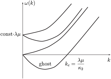
Figure 1: Dispersion relations $\omega(k)$ for vector modes. Not shown are four other frequencies which are mirror symmetric against $\omega=0$, i.e., $\omega\to-\omega$.

$$\omega^{2}(k) \simeq \left[\begin{array}[]{l}(\lambda\mu)^{2}\\ k^{2}\end{array}\right.\ \ \ \ k\ll\lambda\mu$$ (23)

and at

$$k=k_{c}\equiv\frac{\lambda\mu}{\kappa_{2}}\simeq\lambda\mu$$

one of the modes crosses zero and becomes a gapless ghost. The latter fact is obvious from quantum-mechanical viewpoint; it can be also checked by an explicit calculation of the classical energy of a wave: one finds that the energy is negative at $k<k_{c}$. As discussed in Refs. [22, 6], this is phenomenologically acceptable provided that $k_{c}$ is small enough.

3.3 Scalar sector

The analysis of the scalar sector is even simpler. We write for light modes

$$a_{0}^{i}=\frac{\mu}{2}\partial_{i}v,\ \ b_{0}^{i}=\frac{M}{2}\partial_{i}v$$

where $v$ is one of the two light fields, the second being the field $d$. These two fields decouple in the two-derivative Lagrangian $\mathcal{L}_{V}^{(2)}$, while they mix through the one-derivative term $\mathcal{L}_{V}^{(1)}$. The quadratic Lagrangian is then

$$\frac{1}{\mu^{2}}\mathcal{L}^{\mbox{s}}=\nu_{1}(\partial_{0}\partial_{i}d)^{2}-\nu_{2}(\partial_{i}^{2}d)^{2}+\nu_{3}(\partial_{0}\partial_{i}v)^{2}-\nu_{4}(\partial_{i}^{2}v)^{2}-2\lambda\mu\partial_{0}d\cdot\partial_{i}^{2}v$$ (24)

where $\nu_{i}$ are again combinations of the parameters entering $\mathcal{L}_{V}^{(2)}$. At $k\gg\lambda\mu$ the dispersion relations again have the form (18), while at $k\ll\lambda\mu$ the two scalar modes have quite different dispersion relations: one is

$$\omega^{2}\simeq(\lambda\mu)^{2},\ \ \ \ k\ll\lambda\mu$$

and another is

$$\omega^{2}=\frac{\nu_{2}\nu_{4}}{(\lambda\mu)^{2}}k^{4},\ \ \ \ k\ll\lambda\mu$$ (25)

In what follows it will be instructive to keep track of the parameter $\alpha^{B}$, assuming that it is larger than the other parameters in $\mathcal{L}_{V}^{(2)}$. It enters $\nu_{2}$ only, so the dispersion relation (25) is, in fact,

$$\omega^{2}\simeq\frac{\alpha^{B}}{(\lambda\mu)^{2}}k^{4},\ \ \ \ k\ll\lambda\mu$$ (26)

As before, the sign “$\simeq$” means that we omit a prefactor of order 1.

Notice that the dispersion relation (26) is similar to the dispersion relation in the ghost condensate model, but, unlike in the latter, it holds at low 3-momenta only. Note also that there are no ghosts or tachyons in the scalar sector even at $k\ll\lambda\mu$.

4 Spectrum with gravity

4.1 Light fields

Once gravity is turned on, in addition to perturbations of the vector fields, Eq. (13), one considers also metric perturbations, $g_{\mu\nu}=\eta_{\mu\nu}+h_{\mu\nu}$. Under the gauge transformations of the general covariance, the perturbations transform as follows,

$$\delta a^{a\mu} = \mu\partial_{a}\xi^{\mu}$$

$$\delta b^{\mu} = -M\partial_{0}\xi^{\mu}$$

$$\delta h_{\mu\nu} = \partial_{\mu}\xi_{\nu}+\partial_{\nu}\xi_{\mu}$$

There are three local gauge-invariant combinations with no derivatives, $(\mu h_{ij}-a_{i}^{j}-a_{j}^{i})$, $(Mh_{00}+2b_{0})$ and $(M\mu h_{0i}-Ma_{0}^{i}+\mu b_{i})$. It is these combinations that can enter the quadratic part of the potential $V$. Indeed, one finds at quadratic order

$$V\!=\!\lambda_{1}\mu^{2}(\mu h_{ii}-2a^{i}_{i})^{2}\!+\lambda_{4}\mu^{2}(\mu h_{ij}-a_{i}^{j}-a_{j}^{i})^{2}\!+\lambda_{2}M^{2}(Mh_{00}+2b_{0})^{2}+\!\lambda_{3}\left(M\mu h_{0i}-Ma^{i}_{0}+\mu b_{i}\right)^{2}$$ (27)

Thus, the light fields can be parametrized by the five combinations, two given by (15) and others being $h_{ij},h_{0i}$ and $h_{00}$, while light components of other fields are expressed through these five (e.g., $a_{i}^{j}+a_{j}^{i}=\mu h_{ij}$).

The decomposition of $h_{\mu\nu}$ similar to (16), reads

$$h_{ij} = \chi_{ij}+\partial_{i}s_{j}+\partial_{j}s_{i}+\partial_{i}\partial_{j}\sigma+\delta_{ij}\tau$$

$$h_{0i} = u_{i}+\partial_{i}\zeta$$

$$h_{00} = \varphi$$

where $\chi_{ij}$ is transverse-traceless, while $s_{i}$ and $u_{i}$ are transverse. The convenient choice of gauge is

$$s_{i}=0,\ \ \ \ \zeta=v=0$$ (28)

By gauge invariance of the original action, the same number of fields (one transverse vector and two scalars) must be non-propagating; these are $u_{i}$, $\varphi$ and $\sigma$. The former two enter the action without time derivatives, while $\sigma\simeq(1/\partial_{i}^{2})\tau$ due to equations of motion.

The analysis of the spectrum is tedious but straightforward. Let us summarize the results.

4.2 Tensors

In the tensor sector, the quadratic Lagrangian is

$$\mathcal{L}^{\mbox{\tiny T}}=\frac{M_{0}^{2}}{2}(\partial_{0}\chi_{ij})^{2}-\frac{M_{1}^{2}}{2}(\partial_{k}\chi_{ij})^{2}+\frac{\lambda\mu^{3}}{4}\varepsilon_{abi}\partial_{i}\chi_{ka}\cdot\chi_{kb}$$

where $M_{0}^{2},M_{1}^{2}=M_{Pl}^{2}+O(\mu^{2})$, and the last term is due to the one-derivative part $\mathcal{L}_{V}^{(1)}$ in the vector Lagrangian. Thus, in the tensor sector, only the scale $\Lambda_{(2)}=\lambda\mu^{3}/M_{Pl}^{2}$ is relevant. Above this scale, the dispersion law is almost standard,

$$\omega^{2}=\mathrm{v_{\mbox{\tiny T}}}^{2}\cdot k^{2},\ \ \ \ k\gg\Lambda_{(2)}$$

where $\mathrm{v_{\mbox{\tiny T}}}=1+O(\mu^{2}/M_{Pl}^{2})$. Below the scale $\Lambda_{(2)}$, the dispersion relation is

$$\omega^{2}\simeq\pm\Lambda_{(2)}\cdot k,\ \ \ \ k\ll\Lambda_{(2)}\equiv\frac{\lambda\mu^{3}}{M_{Pl}^{2}}$$

Minus sign here corresponds to tachyon. One of the tensor modes becomes unstable at $k\simeq\Lambda_{(2)}$.

4.3 Vectors

In the vector sector, one eliminates the non-dynamical field $u_{i}$ by making use of its equation of motion. Then a new term appears in the quadratic Lagrangian,

$$\frac{1}{\mu^{2}}\triangle\mathcal{L}^{\mbox{vec}}\simeq-\frac{\lambda^{2}\mu^{4}}{M_{Pl}^{2}}v_{i}^{2}$$ (29)

The coefficients of already existing terms (17) receive corrections of order $\mu^{2}/M_{Pl}^{2}$. The latter property is not harmless: to avoid tachyons in finite, albeit narrow, momentum range around $k\sim\lambda\mu$, one has to modify the fine-tuning relation (20) by $M_{Pl}$-suppressed corrections.

The term (29) becomes comparable to one-derivative terms in (17) at $k\sim\Lambda_{(2)}$. Therefore, the spectrum (23), with light ghost, persists down to the scale $\Lambda_{(2)}$. At lower momenta the dispersion relations of the gapless modes are

$$\omega^{2}\simeq\mp\Lambda_{(2)}\cdot k,\ \ \ \ k\ll\Lambda_{(2)}$$

while the other two modes still have $\omega^{2}=(\lambda\mu)^{2}$. The ghost existing in the vector sector at $k\lesssim\lambda\mu$ becomes tachyonic at $k\simeq\Lambda_{(2)}$.

4.4 Scalars

The Lagrangian in the scalar sector, in the gauge (28), is

$$\mathcal{L}^{\mbox{s}} = \nu_{1}\mu^{2}(\partial_{0}\partial_{i}d)^{2}-\nu_{2}\mu^{2}(\partial_{i}\partial_{k}d)^{2}+\frac{1}{4}\nu_{3}\mu^{2}(\partial_{i}\varphi)^{2}-\frac{1}{4}\nu_{4}\mu^{2}(\partial_{i}^{2}\partial_{0}\sigma)^{2}+\lambda\mu^{3}\partial_{i}d\cdot\partial_{i}\varphi$$ (30)

$$- 2\lambda\mu^{3}\partial_{i}d\cdot\partial_{i}\tau-3\tilde{M}_{1}^{2}(\partial_{0}\tau)^{2}+\tilde{M}_{2}^{2}(\partial_{i}\tau)^{2}-2\tilde{M}_{3}^{2}\partial_{i}\tau\cdot\partial_{i}\varphi-2\tilde{M}_{4}^{2}\partial_{0}\tau\cdot\partial_{0}\partial_{i}^{2}\sigma$$

where $\nu_{i}$ are the same as in (24), and $\tilde{M}_{i}^{2}=M_{Pl}^{2}+O(\mu^{2})$. The field $\varphi$ is not dynamical indeed, while $\partial_{i}^{2}\sigma$ is algebraically expressed through $\tau$ via its equation of motion. While the gauge (28) is convenient for calculating the spectrum in the general case, the limit $M_{Pl}\to\infty$ is somewhat tricky. One way to proceed is to express $\sigma$ and $\tau$ through $\varphi$ and $d$ using $\sigma$- and $\varphi$-equations, and then plug these $\sigma$ and $\tau$ into $d$- and $\tau$-equations. The resulting system for $d$ and $\varphi$ coincides, in the limit $M_{Pl}\to\infty$, with the field equations obtained from the Lagrangian (24), if one identifies $\varphi$ with $(-2\partial_{0}v)$.

The spectrum corresponding to the Lagrangian (30) coincides with that discussed in section 3.3 down to the momentum scale $\Lambda_{(1)}=\lambda\mu^{2}/M_{Pl}$. At this scale the dispersion relation of the soft mode (26) changes to

$$\omega^{2}\simeq\frac{\alpha^{B}\mu^{2}}{M_{Pl}^{2}}\cdot k^{2},\ \ \ \ k\ll\Lambda_{(1)}\equiv\lambda\frac{\mu^{2}}{M_{Pl}}$$ (31)

These waves propagate in the usual way, but their velocity is small.

To end up this section, we note that the parameter $\alpha^{B}$ appears in the scalar sector only; neither the momentum scales nor dispersion relations depend on $\alpha^{B}$ in the tensor and vector sectors.

5 Gravity of static source

With the Lagrangian (30), it is straightforward to couple $h_{00}\equiv\varphi$ to static source $T_{00}$ and calculate the gravitational field. The result is

$$\varphi = \frac{c_{1}M_{Pl}^{2}\triangle-4\lambda^{2}\mu^{4}}{c_{1}M_{Pl}^{2}\triangle-3\lambda^{2}\mu^{4}}\times\frac{1}{2\hat{M}_{Pl}^{2}\triangle}T_{00}$$

$$\tau = \varphi+\frac{2\lambda^{2}\mu^{4}}{c_{2}M_{Pl}^{2}\triangle-3\lambda^{2}\mu^{4}}\times\frac{1}{2\hat{M}_{Pl}^{2}\triangle}T_{00}$$ (32)

where $\triangle\equiv\partial_{i}^{2}$, $c_{1},c_{2}=1+O(\mu^{2}/M_{Pl}^{2})$ and $\hat{M}_{Pl}^{2}=M_{Pl}^{2}+O(\mu^{2})$. These potentials coincide with the GR expressions at $r\ll\Lambda_{(1)}^{-1}$ (with the “Newton’s law Plank mass” $\hat{M}_{Pl}$), and at large distances tend to the (scalar-tensor) expressions of the Fierz–Pauli theory in the vDVZ limit,

$$\begin{array}[]{l}\varphi=\displaystyle\frac{2}{3}\frac{1}{\hat{M}_{Pl}^{2}\triangle}T_{00}\\ \\ \tau=\displaystyle\frac{1}{3}\frac{1}{\hat{M}_{Pl}^{2}\triangle}T_{00}\end{array},\ \ \ \ r\gg\Lambda_{(1)}^{-1}$$

The corresponding time scale can be obtained from the dispersion relation (31), which at $k\sim\Lambda_{(1)}$ gives

$$\omega^{-1}(k\sim\Lambda_{(1)})\simeq\frac{1}{\Lambda_{(2)}\sqrt{\alpha^{B}}}$$ (33)

For $\alpha^{B}\sim 1$ this scale coincides with the time scale at which the tachyonic instability develops in the tensor and vector sectors. If, on the other hand, one takes $\alpha^{B}$ large, the time scale (33) at which GR is violated gets smaller than the tachyonic time scale $\Lambda_{(2)}^{-1}$. Modification of Newton’s law may occur earlier than the flat space becomes unstable.

6 Cosmological evolution

Finally, let us consider our model in the cosmological context, assuming that the Universe is spatially flat. The metric is

$$ds^{2}=N^{2}(t)dt^{2}-a^{2}(t)dx_{i}^{2}$$ (34)

The potential (9) does not have flat directions respecting the residual $SO(3)$ symmetry, so at late times it is consistent to set the vector fields to their condensate values (in locally Minkowski frame), i.e.,

$$B_{0}=N(t)\cdot M$$

$$A_{i}^{a}=a(t)\cdot\mu\delta_{i}^{a}$$

Plugging these expressions back into the action (7), one evaluates the action in terms of the lapse function $N(t)$ and scale factor $a(t)$. One finds that all terms in the action have one and the same form, so that the total action is

$$S^{\mbox{\tiny cosm}}={\left(M_{Pl}^{\mbox{\tiny cosm}}\right)^{2}}\int\limits\!dt\frac{1}{N}\left(\frac{\dot{a}}{a}\right)^{2}$$ (35)

where $(M_{Pl}^{\mbox{\tiny cosm}})^{2}=M_{Pl}^{2}+O(\mu^{2})$. The form of the action (35) coincides with that of GR, so the cosmological evolution in our model is governed by the standard Friedmann equation. The only peculiarity is that the “cosmological Planck mass” $M_{Pl}^{\mbox{\tiny cosm}}$ in general does not coincide with the “Newton’s law Planck mass” $\hat{M}_{Pl}$ entering (32); this property has been observed in Refs. [16, 17] in a similar context.

This result appears to be of rather general nature (cf. Ref. [18]), at least in four-dimensional theories obeying locality in time and allowing for derivative expansion of the action. The spatially flat, homogeneous and isotropic metric is symmetric under time reparametrizations and space dilations,

$$t\to t^{\prime}(t)$$

$$x^{i}\to\lambda x^{i}$$

With matter fields settled down at their vacuum values (in locally Minkowski frame), the only terms in the action which are local in time, consistent with these symmetries and have not more than two time derivatives are (35) and $\int\limits Ndt$, the latter having the same form as the cosmological constant term. No matter what condensates are there in the Universe, its evolution proceeds according to the Friedmann equation (possibly with modified Newton’s and cosmological constants), provided that the condensates are time-independent (in locally Minkowski frame) and consistent with homogeneity and isotropy of space.

This observation is not entirely trivial. In our model, the energy-momentum tensor of the vector condensates, calculated by making use of the vector Lagrangian (8), (9), (10), is non-zero. The point is that in the spatialy flat, homogeneous and isotropic Universe it is necessarily proportional to the Einstein tensor (and in general also $g_{\mu\nu}$ and terms with higher time derivatives). This results in the appearance of $M_{Pl}^{\mbox{\tiny cosm}}$ instead of $M_{Pl}$ in the action (35).