Deformed PP-waves from the Lunin-Maldacena Background

Abstract:

In this article we study a pp-wave limit of the Lunin-Maldacena background. We show that the relevant string theory background is a homogeneous pp-wave. We obtain the string spectrum. The dual field theory is a deformation of ${\cal N}=4$ super Yang-Mills theory. We have shown that, for a class of operators, at $O(g_{YM}^{2})$ and at leading order in $N$, all contributions to the anomalous dimension come from $F$-terms. We are able to identify the operator in the deformed super Yang-Mills which is dual to the lowest string mode. By studying the undeformed theory we are able to provide some evidence, directly in the field theory, that a small set of nearly protected operators decouple. We make some comments on operators in the Yang-Mills theory that are dual to excited string modes.

1 Introduction

The AdS/CFT correspondence[1] relates string theory on negatively curved spacetime and large $N$ quantum field theories. The correspondence is a strong/weak coupling duality in the ’t Hooft coupling of the field theory. At large $N$ and large ’t Hooft coupling, both quantum gravity and curvature corrections in the string theory are supressed. The dual gauge theory however is strongly coupled. For small ’t Hooft coupling and large $N$, the gauge theory coupling is small, but curvature corrections in the string theory are not. Computations that can be carried out on both sides of the correspondence necessarily involve quantities that are not corrected or receive small corrections, allowing weak coupling results to be extrapolated to strong coupling. A very interesting class of observables of this type are the near BPS operators discovered by Berenstein, Maldacena and Nastase[2], which are dual to excited string modes. Indeed, since these operators are not BPS, the BMN limit of the gauge theory reproduces genuinely stringy physics, via the AdS/CFT correspondence.

In a recent article[3], Lunin and Maldacena (LM) have studied $\beta$-deformations of the ${\cal N}=4$ super Yang-Mills theory, and have identified the corresponding gravitational deformation of the AdS${}_{5}\times$S⁵ background. The field theory deformation is obtained by making the following replacement in the superpotential

$$\mbox{Tr\,}\left(\hat{\Phi}^{1}\hat{\Phi}^{2}\hat{\Phi}^{3}-\hat{\Phi}^{1}\hat{\Phi}^{3}\hat{\Phi}^{2}\right)\to\mbox{Tr\,}\left(e^{i\pi\gamma}\hat{\Phi}^{1}\hat{\Phi}^{2}\hat{\Phi}^{3}-e^{-i\pi\gamma}\hat{\Phi}^{1}\hat{\Phi}^{3}\hat{\Phi}^{2}\right).$$ (1)

The deformed field theory has ${\cal N}=1$ supersymmetry and is invariant under a $U(1)\times U(1)$ non-${\cal R}$ symmetry. The ${\cal N}=4$ theory is dual to string theory in the AdS${}_{5}\times$S⁵ geometry, which contains a two torus. The isometries of the two torus match with the $U(1)\times U(1)$ field theory symmetry. Denote the metric of this two torus by $g$ and the NS-NS two form (which is of course zero in the undeformed theory) by $B$. The deformation of the dual gravitational theory is obtained by replacing

$$\tau=B+i\sqrt{g}\to\tau_{\gamma}={\tau\over 1+\gamma\tau}.$$

The AdS₅ factor is unchanged which is expected because (1) is a marginal deformation. Studies of the AdS/CFT correspondence for this deformation are likely to produce interesting results for at least two reasons. Firstly, it is important to generalize the AdS/CFT correspondence to less supersymmetric examples. Secondly, since this background has a continuous adjustable deformation parameter, it may be possible to define new scaling limits.

A study of semiclassical string states provided important insights into the BMN limit[4]. Motivated by this, semiclassical string states in the LM background were recently compared to a class of gauge theory scalar operators[5]. The 1-loop anomalous dimensions of these operators are described by an integrable spin chain and match beautifully with the energies of the semiclassical string states. Further, by employing the Lax pair for strings in the LM background[6], the Landau-Lifschitz action associated to the one-loop spin chain was recovered. This indicates that the integrable structures in the gauge theory and the string theory match. Further analysis of the relevant spin chain is given in [7]. For further recent insights into the gauge/string correspondence for these (and other) new examples see[8].

The logic employed by Lunin and Maldacena to obtain the gravitational theory dual to the deformed field theory can be extended in a number of ways. Recently, instead of deforming the ${\cal N}=4$ super Yang-Mills theory, deformations of ${\cal N}=1$ and ${\cal N}=2$ theories have been considered[9]. Further, deformations of eleven dimensional geometries of the form AdS${}_{4}\times$Y₇ with $Y_{7}$ a seven dimensional Sasaki-Einstein[10],[11] or weak $G_{2}$ or tri-Sasakian[11] space have been considered.

In this article we are interested in studying a pp-wave limit of the LM background. There are a number of interesting pp-wave limits that can be taken. Each of these limits allows us to probe different stringy aspects of the correspondence, and are thus worthy of study. One such limit was in fact already considered in [12]. We will be considering a different pp-wave limit, to provide further independent support for and insight into the correspondence of [3].

The paper is organized as follows: in section 2 we describe the pp-wave limit that we consider here. We obtain the metric and B field by taking an appropriate limit of the results in [3]. The resulting background is a homogeneous pp-wave[13]. It is known that the string sigma model in this background can be solved exactly[14]. We provide this analysis in section 3. In section 4 we study the dual gauge theory and consider the question of how to define the near-BPS operators with anomalous dimensions which reproduce the spectrum of the string sigma model. We are able to argue that, in the large $N$ limit and at one loop, one can ignore gluon exchange, self energy insertions and $D$-term contributions. This allows a significant simplification of the analysis. We are able to identify the operator dual to the lowest string mode. For $\gamma=0$ we are able to find near-BPS operators which reproduce the spectrum of the string sigma model. Our results are consistent with the expected decoupling of a small set of nearly protected operators. In the $\gamma\neq 0$ case, we are able argue that there is a set of nearly protected operators whose spectrum of anomalous dimensions is independent of $\gamma$ in agreement with the string theory result. We also find near BPS operators for small values of the ${\cal R}$ charge $J$ and find that their anomalous dimension does depend on $\gamma$. Section 5 is reserved for a discussion of our results.

2 PP-wave Limit of the Lunin-Maldacena Geometry

In this section we will take the pp-wave limit of the LM background. Our goal is to obtain the spectrum of free strings in this background. To write down the relevant string sigma model, we need only the metric and the B field. Thus, we do not consider the RR-fluxes $C_{2}$ and $C_{4}$ which are also non-zero in the LM background.

The metric is[3]

$$ds^{2} = R^{2}\left(-dt^{2}\cosh^{2}\rho+d\rho^{2}+\sinh^{2}\rho d\Omega_{3}^{2}+\sum_{i}d\mu_{i}^{2}\right.$$ (2)

$$+ \left.G\sum_{i=1}^{3}\mu_{i}^{2}d\phi_{i}^{2}+\gamma^{2}\mu_{1}^{2}\mu_{2}^{2}\mu_{3}^{2}G\left(\sum_{i}d\phi_{i}\right)^{2}\right).$$

where

$$\mu_{1}=\cos\alpha,\qquad\mu_{2}=\sin\alpha\cos\theta,\qquad\mu_{3}=\sin\alpha\sin\theta,$$

$$G={1\over 1+\gamma^{2}(\mu_{1}^{2}\mu_{2}^{2}+\mu_{1}^{2}\mu_{3}^{2}+\mu_{3}^{2}\mu_{2}^{2})}.$$

It is useful to use the angles $\psi$, $\varphi_{1}$ and $\varphi_{2}$, defined by

$$\phi_{1}=\psi-\varphi_{2},\qquad\phi_{2}=\psi+\varphi_{1}+\varphi_{2},\qquad\phi_{3}=\psi-\varphi_{1}.$$

The parameter $\gamma$ is the deformation parameter. We will perform the Penrose limit using the null geodesic $\tau=\psi$, with $\alpha_{0}=\cos^{-1}{1\over\sqrt{3}}$ and $\theta_{0}={\pi\over 4}.$ We set

$$\theta={\pi\over 4}+\sqrt{2\over 3}{x^{1}\over R},\qquad\alpha=\alpha_{0}-{x^{2}\over R},\qquad\rho={r\over R}$$

$$\varphi_{1}={x^{3\prime}\over R},\qquad\varphi_{2}={x^{4\prime}\over R},\qquad t=x^{+}+{x^{-}\over R^{2}},\qquad\psi={x^{-}\over R^{2}}-x^{+},$$

$$x^{3}=\sqrt{2\over 3+\gamma^{2}}\left(x^{3\prime}+{1\over 2}x^{4\prime}\right),\qquad x^{4}=\sqrt{3\over 2(3+\gamma^{2})}x^{4\prime},$$

and take the limit $R\to\infty$. The pp-wave metric we obtain is

$$ds^{2} = -4dx^{+}dx^{-}-\left[r^{2}+{4\gamma^{2}\over 3+\gamma^{2}}\left((x^{1})^{2}+(x^{2})^{2}\right)\right](dx^{+})^{2}+dr^{2}+r^{2}d\Omega_{3}^{2}$$ (3)

$$+ (dx^{1})^{2}+(dx^{2})^{2}+(dx^{3})^{2}+(dx^{4})^{2}+{4\sqrt{3}\over\sqrt{3+\gamma^{2}}}\left(x^{1}dx^{3}+x^{2}dx^{4}\right)dx^{+}.$$

To obtain the string sigma model, we will also need the $B$ field in the pp-wave limit. We find

$$B_{\varphi_{1}\varphi_{2}}{\cal D}\varphi_{1}\wedge{\cal D}\varphi_{2}=G\gamma gR^{2}{\cal D}\varphi_{1}\wedge{\cal D}\varphi_{2},$$

where

$${\cal D}\varphi_{1}=d\varphi_{1}-d\psi+{3\mu_{1}^{2}\mu_{2}^{2}\over g}d\psi,\qquad{\cal D}\varphi_{2}=d\varphi_{2}-d\psi+{3\mu_{3}^{2}\mu_{2}^{2}\over g}d\psi.$$

Taking the pp-wave limit as above, we find the following $B$ field

$$B={\gamma\over\sqrt{3}}dx^{3}\wedge dx^{4}+{2\gamma\over\sqrt{3+\gamma^{2}}}(x^{2}dx^{3}\wedge dx^{+}+x^{1}dx^{+}\wedge dx^{4}),$$

and the following field strengths

$$H_{23+}={2\gamma\over\sqrt{3+\gamma^{2}}},\qquad H_{14+}=-{2\gamma\over\sqrt{3+\gamma^{2}}}.$$

Thus, the field strength is null as it should be in the pp-wave limit.

3 Strings in the PP-wave Limit of the Lunin-Maldacena Geometry

Given the metric and $B$ fields written down in the previous section, in this section we consider the resulting string sigma model. We show that this background corresponds to a homogeneous pp-wave[13] and are thus able to use existing results[14] to obtain the spectrum.

We will be working in lightcone gauge. The string worldsheet action is (we are dropping the fermions from our analysis)

$$S=-{1\over 4\pi\alpha^{\prime}}\int d^{2}\sigma\left[\sqrt{\eta}\eta^{ab}g_{\mu\nu}\partial_{a}X^{\mu}\partial_{b}X^{\nu}+\epsilon^{ab}B^{NS}_{\mu\nu}\partial_{a}X^{\mu}\partial_{b}X^{\nu}+\alpha^{\prime}\sqrt{\eta}\phi(x)R\right],$$

with $R$ the scalar curvature on the worldsheet, $\eta^{ab}$ is the worldsheet metric and $\eta=|\det{\eta_{ab}}|$. We will choose $\sqrt{\eta}\eta^{ab}$ diagonal with $\sqrt{\eta}\eta^{00}=-1$ and $\sqrt{\eta}\eta^{11}=1$. After shifting

$$x^{-}\to x^{-}+{\sqrt{3}\over 2\sqrt{3+\gamma^{2}}}(x^{1}x^{3}+x^{2}x^{4}),$$

the metric becomes

$$ds^{2} = -4dx^{+}dx^{-}-\left[\sum_{i=5}^{8}(x^{i})^{2}+{4\gamma^{2}\over 3+\gamma^{2}}\left((x^{1})^{2}+(x^{2})^{2}\right)\right](dx^{+})^{2}$$

$$+ \sum_{i=1}^{8}(dx^{i})^{2}+{2\sqrt{3}\over\sqrt{3+\gamma^{2}}}\left(x^{1}dx^{3}-x^{3}dx^{1}+x^{2}dx^{4}-x^{4}dx^{2}\right)dx^{+}.$$

This metric corresponds to a homogeneous pp-wave[13]. The sigma model for this background has been considered in [14]; we will review the relevant results here. In the gauge $x^{+}=\tau$, we obtain the following Lagrangian density (we take $\sigma$ to run from $0$ to $\pi$ and set $\alpha^{\prime}={1\over 2\pi}$)

$${\cal L} = -2{\partial x^{-}\over\partial\tau}-{1\over 2}\left[\sum_{i=5}^{8}(x^{i})^{2}+{4\gamma^{2}\over 3+\gamma^{2}}((x^{1})^{2}+(x^{2})^{2})\right]+{2\gamma\over\sqrt{3+\gamma^{2}}}\left(x^{2}{\partial x^{3}\over\partial\sigma}-x^{1}{\partial x^{4}\over\partial\sigma}\right)$$

$$+ {\sqrt{3}\over\sqrt{3+\gamma^{2}}}\left(x^{1}{\partial x^{3}\over\partial\tau}-x^{3}{\partial x^{1}\over\partial\tau}+x^{2}{\partial x^{4}\over\partial\tau}-x^{4}{\partial x^{2}\over\partial\tau}\right)-{1\over 2}\sum_{i=1}^{8}\partial_{a}x^{i}\partial^{a}x^{i}.$$

To quantize the theory, compute the canonical momenta

$$p^{1}(\tau,\sigma)=\dot{x}^{1}(\tau,\sigma)-\sqrt{3\over 3+\gamma^{2}}x^{3},\qquad p^{2}(\tau,\sigma)=\dot{x}^{2}(\tau,\sigma)-\sqrt{3\over 3+\gamma^{2}}x^{4},$$

$$p^{3}(\tau,\sigma)=\dot{x}^{3}(\tau,\sigma)+\sqrt{3\over 3+\gamma^{2}}x^{1},\qquad p^{4}(\tau,\sigma)=\dot{x}^{4}(\tau,\sigma)+\sqrt{3\over 3+\gamma^{2}}x^{2},$$

$$p^{k}(\tau,\sigma)={\partial{\cal L}\over\partial\dot{x}^{k}}=\dot{x}^{k}(\tau,\sigma)\qquad k=5,6,7,8,$$

and impose the equal time commutation relations

$$\big{[}p^{k}(\tau,\sigma),x^{j}(\tau,\sigma^{\prime})\big{]}=-i\delta^{jk}\delta(\sigma-\sigma^{\prime}).$$

The Hamiltonian is

$$H={1\over 2}\int_{0}^{\pi}d\sigma\left[\sum_{k=1}^{8}\left(p^{k}p^{k}+{\partial x^{k}\over\partial\sigma}{\partial x^{k}\over\partial\sigma}\right)+{3\over 3+\gamma^{2}}\sum_{k=1}^{4}(x^{k})^{2}+\sum_{k=5}^{8}(x^{k})^{2}+{4\gamma^{2}\over 3+\gamma^{2}}\sum_{k=1}^{2}(x^{k})^{2}\right.$$

$$\left.-{4\gamma\over\sqrt{3+\gamma^{2}}}\left(x^{2}{\partial x^{3}\over\partial\sigma}-x^{1}{\partial x^{4}\over\partial\sigma}\right)+{2\sqrt{3}\over\sqrt{3+\gamma^{2}}}\left(p^{1}x^{3}+p^{2}x^{4}-p^{3}x^{1}-p^{4}x^{2}\right)\right].$$

Notice that the modes corresponding to $x^{5},x^{6},x^{7},x^{8}$ have masses that do not depend on $\gamma$, i.e. they are unaffected by the deformation. This is not unexpected, since these coordinates come from the AdS₅ part of the space which does not participate in the deformation. We will, from this point on, consider only $x^{1},x^{2},x^{3},x^{4}$.

The Heisenberg equations of motion are

$${\partial^{2}x^{i}\over\partial t^{2}}-{\partial^{2}x^{i}\over\partial\sigma^{2}}+f^{ij}{\partial x^{j}\over\partial t}+h^{ij}{\partial x^{j}\over\partial\sigma}+k_{i}x^{i}=0,$$

where

$$f^{ij}=\left[\matrix{0&0&-2\sqrt{3\over 3+\gamma^{2}}&0\cr 0&0&0&-2\sqrt{3\over 3+\gamma^{2}}\cr 2\sqrt{3\over 3+\gamma^{2}}&0&0&0\cr 0&2\sqrt{3\over 3+\gamma^{2}}&0&0}\right],$$

and

$$h^{ij}=2\left[\matrix{0&0&0&{\gamma\over\sqrt{3+\gamma^{2}}}\cr 0&0&-{\gamma\over\sqrt{3+\gamma^{2}}}&0\cr 0&{\gamma\over\sqrt{3+\gamma^{2}}}&0&0\cr-{\gamma\over\sqrt{3+\gamma^{2}}}&0&0&0}\right],$$

$$k_{1}=k_{2}={4\gamma^{2}\over 3+\gamma^{2}},\qquad k_{3}=k_{4}=0.$$

To solve these equations introduce the mode expansions

$$x^{i}(t,\sigma)=\sum_{n=-\infty}^{\infty}x_{n}^{i}(t)e^{2in\sigma}.$$

Reality of $x^{i}(t,\sigma)$ is encoded (as usual) in

$$x_{n}^{i}=(x_{-n}^{i})^{*}.$$

The equations of motion now become the following equation for the modes

$${\partial^{2}x^{i}_{n}\over\partial t^{2}}+4n^{2}x^{i}_{n}+f^{ij}{\partial x^{j}_{n}\over\partial t}+2inh^{ij}x^{j}_{n}+k_{i}x^{i}_{n}=0.$$

Following [14] we now make the following ansatz

$$x_{n}^{i}(t)=a^{(n)}_{j}A^{(n)}_{ij}e^{i\omega^{(n)}_{j}t}.$$

$a^{(n)}_{j}$ will be a destruction/annihilation operator; $A^{(n)}_{ij}$ is a unitary transformation diagonalizing the equation of motion; $\omega^{(n)}_{j}$ is our spectrum. Plugging this into the equations of motion we find

$$\left(-(\omega_{k}^{(n)})^{2}\delta^{ij}+4n^{2}\delta^{ij}+if^{ij}\omega_{k}^{(n)}+2inh^{ij}+k_{i}\delta^{ij}\right)a_{k}^{(n)}A_{jk}^{(n)}e^{i\omega_{k}^{(n)}t}=0.$$

The condition for a nontrivial solution is

$$\det\left(-(\omega_{k}^{(n)})^{2}\delta^{ij}+4n^{2}\delta^{ij}+if^{ij}\omega_{k}^{(n)}+2inh^{ij}+k_{i}\delta^{ij}\right)=0,$$

which leads to the following quartic equation

$$\omega^{4}-(4+8n^{2})\omega^{2}+16n^{4}=0.$$

It is solved by

$$\omega=1\pm\sqrt{1+4n^{2}}.$$

This is in perfect agreement with [15]. Notice that the spectrum is independent of the deformation parameter $\gamma$. The fact that the spectrum is independent of $\gamma$ is unexpected. Evidently, the $\gamma$ dependence in the $B$ field exactly compensates for the $\gamma$ dependence of the geometry.

4 Dual Field Theory Analysis

In this section, we will study the field theory obtained after deforming the superpotential (fields with a hat $\hat{\Phi}$ denote superfields; fields without a hat $\Phi$ denote the Higgs fields - the bosonic bottom component of $\hat{\Phi}$)

$$\mbox{Tr\,}\left(\hat{\Phi}^{1}\hat{\Phi}^{2}\hat{\Phi}^{3}-\hat{\Phi}^{1}\hat{\Phi}^{3}\hat{\Phi}^{2}\right)\to\mbox{Tr\,}\left(e^{i\pi\gamma}\hat{\Phi}^{1}\hat{\Phi}^{2}\hat{\Phi}^{3}-e^{-i\pi\gamma}\hat{\Phi}^{1}\hat{\Phi}^{3}\hat{\Phi}^{2}\right).$$

We consider only the Higgs fields. Our goal is to construct operators dual to the string modes discussed in section 3.1; these will be built from the Higgs fields. The kinetic terms and $D$ terms for the Higgs fields are invariant under the deformation. The usual $F$ terms are however now replaced by

$$V=\mbox{Tr\,}(\Big{|}\big{[}\Phi^{2},\Phi^{3}\big{]}_{\gamma}\Big{|}^{2}+\Big{|}\big{[}\Phi^{3},\Phi^{1}\big{]}_{\gamma}\Big{|}^{2}+\Big{|}\big{[}\Phi^{1},\Phi^{2}\big{]}_{\gamma}\Big{|}^{2}),$$

where

$$\big{[}A,B\big{]}_{\gamma}\equiv e^{i\pi\gamma}AB-e^{-i\pi\gamma}BA.$$

In the undeformed theory[16], when computing correlators of traces in the case that each trace involves only $\Phi^{1}$, $\Phi^{2}$ and $\Phi^{3}$ or $\bar{\Phi}^{1}$, $\bar{\Phi}^{2}$ and $\bar{\Phi}^{3}$, one does not need to consider $D$-term contributions, self energy corrections or gluon exchange at order $g_{YM}^{2}$ in Yang-Mills perturbation theory. (See [17] for useful superspace techniques.) We will argue that this is also true in the deformed theory, at leading order in $N$. Using this insight, we construct operators in the Yang-Mills theory that are dual to the vacuum of the sigma model. Next we study operators dual to excited string states in the undeformed ($\gamma=0$) theory. Finally, we reconsider this question in the deformed theory.

4.1 Only $F$-terms contribute

In this section we will consider correlators of the form

$$\langle{\cal O}\bar{\cal O}\rangle,$$

where ${\cal O}$ is a trace of $k$ Higgs fields

$${\cal O}=f_{i_{1}i_{2}\cdots i_{k}}\mbox{Tr\,}\left(\Phi^{i_{1}}\Phi^{i_{2}}\cdots\Phi^{i_{k}}\right),$$

and the indices $i_{1},...,i_{k}\in\{1,2,3\}$. We do not assume anything about the coefficient $f_{i_{1}i_{2}\cdots i_{k}}$. In the undeformed theory[16], one argues that the $D$-terms, gluon exchange and self energy corrections are all flavor blind at one-loop. Consequently, if we are working to one loop order, we could replace

$${\cal O}\to\mbox{Tr\,}\left((\Phi^{1})^{k}\right).$$

The result of [18] tells us that the correlator $\langle\mbox{Tr\,}\left((\Phi^{1})^{k}\right)\mbox{Tr\,}\left((\bar{\Phi}^{1})^{k}\right)\rangle$ receives no radiative corrections at $O(g_{YM}^{2})$, so the result follows.

When we deform the theory, the $D$-term contributions and gluon exchange contributions are unchanged. $F$-term contributions to the self energy need to be considered carefully because the $F$-terms are affected by the deformation. The $F$-terms can be split into two pieces

$$V_{F}=V_{inv}+V_{def},$$

where

$$V_{inv}=2\mbox{Tr\,}(\Phi^{1}\Phi^{2}\bar{\Phi}^{2}\bar{\Phi}^{1}+\Phi^{2}\Phi^{1}\bar{\Phi}^{1}\bar{\Phi}^{2}),$$

$$V_{def}=-2\mbox{Tr\,}(e^{-2\pi i\gamma}\Phi^{2}\Phi^{1}\bar{\Phi}^{2}\bar{\Phi}^{1}+e^{2\pi i\gamma}\Phi^{1}\Phi^{2}\bar{\Phi}^{1}\bar{\Phi}^{2}).$$

The self energy contribution coming from $V_{inv}$ will be the same as in the undeformed theory; self energy contribution coming from $V_{def}$ will not. The Feynman diagrams corresponding to self energy contributions, coming from these two vertices, are shown below. (A) shows the contribution from $V_{inv}$ and (B) the contribution from $V_{def}$. Since (B) is a non-planar diagram, it can be dropped at large $N$ and consequently, the only contribution to the self energy coming from the $F$-terms is invariant under the deformation to leading order in $N$. Thus, for the correlators that we are considering, one does not need to consider $D$-term contributions, self energy corrections or gluon exchange, at order $g_{YM}^{2}$ in Yang-Mills perturbation theory and at leading order in $N$.

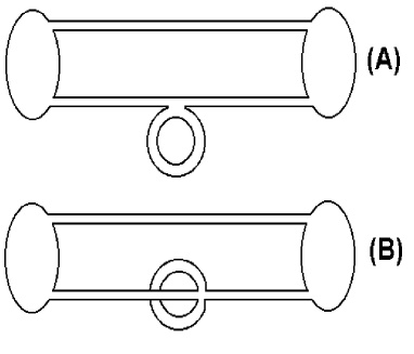
Figure 1: This plot shows the Feynman diagrams corresponding to self energy contributions coming from the $F$-terms. (A) shows the contribution from $V_{inv}$ and (B) the contribution from $V_{def}$. (A) is $O(g_{YM}^{2}N^{3})$; (B) is $O(g_{YM}^{2}N)$.

4.2 Operators dual to the Vacuum

The operator dual to the vacuum of the string sigma model is a BPS operator. Thus, we expect that the $U(1)_{\cal R}$ charge of this operator is equal to its conformal dimension, and further that it is not charged under the $U(1)\times U(1)$ symmetry of the field theory. This follows because our pp-wave limit is taken by boosting along $\psi$; there is no momentum in the $\varphi_{1},\varphi_{2}$ directions. The charges and dimension of the three Higgs fields are

$$\matrix{&U(1)&U(1)&U(1)_{\cal R}\equiv J&\Delta\cr\Phi^{1}&0&-1&1&1\cr\Phi^{2}&1&1&1&1\cr\Phi^{3}&-1&0&1&1}$$

We will explicitly construct the operator dual to the vacuum for small values of $J$. This will allow us to extract a rule that gives the correct operator for all $J$.

For $J=3$, there are two independent loops out of which the operator dual to the vacuum could be constructed

$${\cal O}_{1}=\mbox{Tr\,}(\Phi^{1}\Phi^{2}\Phi^{3}),\qquad{\cal O}_{2}=\mbox{Tr\,}(\Phi^{1}\Phi^{3}\Phi^{2}).$$

Using the two point function of the Higgs fields (indices $a,b,c,d=1,...,N$ are color labels; indices $j,k=1,2,3$)

$$\langle\bar{\Phi}^{j}_{ab}(x)\Phi^{k}_{cd}(0)\rangle=\delta^{jk}\delta_{ad}\delta_{bc}{1\over 4\pi^{2}|x|^{2}}\equiv\delta^{jk}\delta_{ad}\delta_{bc}{a\over|x|^{2}},$$

we compute the planar contribution to

$$\langle\bar{\cal O}_{i}(x_{1})V_{F}(y){\cal O}_{j}(x_{2})\rangle={\cal M}_{ij}{a^{5}\over|x_{1}-y|^{4}|x_{2}-y|^{4}|x_{1}-x_{2}|^{2}}N^{4}.$$ (4)

We use the above correlator to define the matrix ${\cal M}$. The result is

$${\cal M}^{T}=\left[\matrix{6&-6e^{-2\pi i\gamma}\cr-6e^{2\pi i\gamma}&6}\right].$$

The matrix ${\cal M}$ has a single zero eigenvalue. The operator dual to the vacuum is given by that linear combination which corresponds to the zero eigenvalue - it is the two point function of this linear combination that is not corrected, as expected for a BPS operator. There is a single zero eigenvalue which implies that this state is unique. Our operator is

$${\cal O}_{\gamma}=\mbox{Tr\,}\left(\Phi^{1}\Phi^{2}\Phi^{3}\right)+e^{-2\pi i\gamma}\mbox{Tr\,}\left(\Phi^{1}\Phi^{3}\Phi^{2}\right).$$

It has dimension $\Delta=3$, $U(1)_{\cal R}$ charge $J=3$ and is neutral under $U(1)\times U(1)$. Notice that when $\gamma=0$ our deformed operator recovers the expected BPS operator of the undeformed case and further that ${\cal O}_{\gamma}$ respects the $Z_{3}$ symmetry (which acts as a cyclic permutation of the three Higgs fields) of the deformed theory.

Next, consider $J=6$. In this case, our operator is a linear combination of 16 loops

$${\cal O}_{1}=\mbox{Tr\,}\left(\Phi^{1}\Phi^{1}\Phi^{2}\Phi^{2}\Phi^{3}\Phi^{3}\right)\,\,{\cal O}_{2}=\mbox{Tr\,}\left(\Phi^{1}\Phi^{1}\Phi^{2}\Phi^{3}\Phi^{2}\Phi^{3}\right)\,\,{\cal O}_{3}=\mbox{Tr\,}\left(\Phi^{1}\Phi^{1}\Phi^{2}\Phi^{3}\Phi^{3}\Phi^{2}\right)$$

$${\cal O}_{4}=\mbox{Tr\,}\left(\Phi^{1}\Phi^{1}\Phi^{3}\Phi^{2}\Phi^{2}\Phi^{3}\right)\,\,{\cal O}_{5}=\mbox{Tr\,}\left(\Phi^{1}\Phi^{1}\Phi^{3}\Phi^{2}\Phi^{3}\Phi^{2}\right)\,\,{\cal O}_{6}=\mbox{Tr\,}\left(\Phi^{1}\Phi^{1}\Phi^{3}\Phi^{3}\Phi^{2}\Phi^{2}\right)$$

$${\cal O}_{7}=\mbox{Tr\,}\left(\Phi^{1}\Phi^{2}\Phi^{1}\Phi^{2}\Phi^{3}\Phi^{3}\right)\,\,{\cal O}_{8}=\mbox{Tr\,}\left(\Phi^{1}\Phi^{2}\Phi^{1}\Phi^{3}\Phi^{2}\Phi^{3}\right)\,\,{\cal O}_{9}=\mbox{Tr\,}\left(\Phi^{1}\Phi^{2}\Phi^{1}\Phi^{3}\Phi^{3}\Phi^{2}\right)$$

$${\cal O}_{10}=\mbox{Tr\,}\left(\Phi^{1}\Phi^{2}\Phi^{2}\Phi^{1}\Phi^{3}\Phi^{3}\right)\,\,{\cal O}_{11}=\mbox{Tr\,}\left(\Phi^{1}\Phi^{2}\Phi^{2}\Phi^{3}\Phi^{1}\Phi^{3}\right)\,\,{\cal O}_{12}=\mbox{Tr\,}\left(\Phi^{1}\Phi^{2}\Phi^{3}\Phi^{1}\Phi^{2}\Phi^{3}\right)$$

$${\cal O}_{13}=\mbox{Tr\,}\left(\Phi^{1}\Phi^{2}\Phi^{3}\Phi^{1}\Phi^{3}\Phi^{2}\right)\,\,{\cal O}_{14}=\mbox{Tr\,}\left(\Phi^{1}\Phi^{2}\Phi^{3}\Phi^{2}\Phi^{1}\Phi^{3}\right)\,\,{\cal O}_{15}=\mbox{Tr\,}\left(\Phi^{1}\Phi^{3}\Phi^{1}\Phi^{3}\Phi^{2}\Phi^{2}\right)$$

$${\cal O}_{16}=\mbox{Tr\,}\left(\Phi^{1}\Phi^{3}\Phi^{2}\Phi^{1}\Phi^{3}\Phi^{2}\right).$$

These operators were selected by requiring that they have $\Delta=J=6$, and zero $U(1)\times U(1)$ charge. We again want to identify the linear combination of these operators that is BPS. As for the case $J=3$, we do this by looking for the linear combination whose two point function does not receive corrections at $O(g_{YM}^{2})$ and at leading order in $N$. By studying the correlator (4) we can read off ${\cal M}$; null vectors of ${\cal M}$ are then natural candidate BPS operators. In this case, again at leading order in $N$ we find

$${\cal M}^{T}=2\left[\matrix{3&b&0&0&0&0&b&0&0&0&b&0&0&0&0&0\cr b^{*}&5&b&b&0&0&0&b&0&0&0&0&0&b&0&0\cr 0&b^{*}&4&0&b&0&b^{*}&0&b&0&0&0&0&0&0&0\cr 0&b^{*}&0&4&b&0&0&0&0&0&b^{*}&0&0&0&b&0\cr 0&0&b^{*}&b^{*}&5&b&0&b^{*}&0&0&0&0&0&b^{*}&0&0\cr 0&0&0&0&b^{*}&3&0&0&b^{*}&0&0&0&0&0&b^{*}&0\cr b^{*}&0&b&0&0&0&5&b&0&b&0&0&b&0&0&0\cr 0&b^{*}&0&0&b&0&b^{*}&6&b&0&0&b^{*}&0&0&0&b\cr 0&0&b^{*}&0&0&b&0&b^{*}&5&b^{*}&0&0&b^{*}&0&0&0\cr 0&0&0&0&0&0&b^{*}&0&b&4&b^{*}&0&0&0&b&0\cr b^{*}&0&0&b&0&0&0&0&0&b&5&0&b&b&0&0\cr 0&0&0&0&0&0&0&2b&0&0&0&6&2b&2b&0&0\cr 0&0&0&0&0&0&b^{*}&0&b&0&b^{*}&b^{*}&6&0&b&b\cr 0&b^{*}&0&0&b&0&0&0&0&0&b^{*}&b^{*}&0&6&b&b\cr 0&0&0&b^{*}&0&b&0&0&0&b^{*}&0&0&b^{*}&b^{*}&5&0\cr 0&0&0&0&0&0&0&2b^{*}&0&0&0&0&2b^{*}&2b^{*}&0&6}\right]$$

where $b=-e^{-2\pi i\gamma}$ and $b^{*}=-e^{2\pi i\gamma}$. Again, ${\cal M}$ has a single zero eigenvalue, so that there is an operator whose two point function does not get corrected at $O(g_{YM}^{2})$ and it is again unique. For $J=9$ there are 188 basis loops. In this case ${\cal M}$ again has a single null vector, so that we again have a unique candidate BPS operator.

By studying the candidate BPS operators for $J=3,6,9$ we have been able to identify a rule which allows us to write down a candidate BPS operator for any $J$. To write down our rule, we call the following exchanges

$$\Phi^{1}\Phi^{2}\to\Phi^{2}\Phi^{1},\quad{\rm or}\quad\Phi^{2}\Phi^{3}\to\Phi^{3}\Phi^{2},\quad{\rm or}\quad\Phi^{3}\Phi^{1}\to\Phi^{1}\Phi^{3},$$

even exchanges and the exchanges

$$\Phi^{2}\Phi^{1}\to\Phi^{1}\Phi^{2},\quad{\rm or}\quad\Phi^{3}\Phi^{2}\to\Phi^{2}\Phi^{3},\quad{\rm or}\quad\Phi^{1}\Phi^{3}\to\Phi^{3}\Phi^{1},$$

odd exchanges. Consider for illustration the case with $J=6$. To construct the vacuum state, we start from the loop $\mbox{Tr\,}\left(\Phi^{1}\Phi^{1}\Phi^{2}\Phi^{2}\Phi^{3}\Phi^{3}\right)$ and perform a sequence of even and odd exchanges until we generate the full 16 operators generated above. For each odd exchange we append the factor $\alpha^{*}=e^{2\pi\gamma i}$, and for each even exchange we append the factor $\alpha=e^{-2\pi\gamma i}$. Thus, for example, since

$$\mbox{Tr\,}\left(\Phi^{1}\Phi^{1}\Phi^{2}\Phi^{3}\Phi^{3}\Phi^{2}\right)$$

is obtained from

$$\mbox{Tr\,}\left(\Phi^{1}\Phi^{1}\Phi^{2}\Phi^{2}\Phi^{3}\Phi^{3}\right)$$

by performing two even exchanges

$$\mbox{Tr\,}\left(\Phi^{1}\Phi^{1}\Phi^{2}\Phi^{2}\Phi^{3}\Phi^{3}\right)\to\mbox{Tr\,}\left(\Phi^{1}\Phi^{1}\Phi^{2}\Phi^{3}\Phi^{2}\Phi^{3}\right)\to\mbox{Tr\,}\left(\Phi^{1}\Phi^{1}\Phi^{2}\Phi^{3}\Phi^{3}\Phi^{2}\right),$$

we know that it will have a phase of $\alpha^{2}=(e^{-2\pi i\gamma})^{2}$. Following this rule, we find the following operator

$${\cal O}_{def} = \mbox{Tr\,}\left(\Phi^{1}\Phi^{1}\Phi^{2}\Phi^{2}\Phi^{3}\Phi^{3}\right)+\alpha\mbox{Tr\,}\left(\Phi^{1}\Phi^{1}\Phi^{2}\Phi^{3}\Phi^{2}\Phi^{3}\right)$$

$$+ \alpha^{2}\mbox{Tr\,}\left(\Phi^{1}\Phi^{1}\Phi^{2}\Phi^{3}\Phi^{3}\Phi^{2}\right)+\alpha^{2}\mbox{Tr\,}\left(\Phi^{1}\Phi^{1}\Phi^{3}\Phi^{2}\Phi^{2}\Phi^{3}\right)$$

$$+ \alpha^{3}\mbox{Tr\,}\left(\Phi^{1}\Phi^{1}\Phi^{3}\Phi^{2}\Phi^{3}\Phi^{2}\right)+\alpha^{4}\mbox{Tr\,}\left(\Phi^{1}\Phi^{1}\Phi^{3}\Phi^{3}\Phi^{2}\Phi^{2}\right)$$

$$+ \alpha\mbox{Tr\,}\left(\Phi^{1}\Phi^{2}\Phi^{1}\Phi^{2}\Phi^{3}\Phi^{3}\right)+\alpha^{2}\mbox{Tr\,}\left(\Phi^{1}\Phi^{2}\Phi^{1}\Phi^{3}\Phi^{2}\Phi^{3}\right)$$

$$+ \alpha^{3}\mbox{Tr\,}\left(\Phi^{1}\Phi^{2}\Phi^{1}\Phi^{3}\Phi^{3}\Phi^{2}\right)+\alpha^{2}\mbox{Tr\,}\left(\Phi^{1}\Phi^{2}\Phi^{2}\Phi^{1}\Phi^{3}\Phi^{3}\right)$$

$$+ \alpha\mbox{Tr\,}\left(\Phi^{1}\Phi^{2}\Phi^{2}\Phi^{3}\Phi^{1}\Phi^{3}\right)+\alpha\mbox{Tr\,}\left(\Phi^{1}\Phi^{2}\Phi^{3}\Phi^{1}\Phi^{2}\Phi^{3}\right)$$

$$+ \alpha^{2}\mbox{Tr\,}\left(\Phi^{1}\Phi^{2}\Phi^{3}\Phi^{1}\Phi^{3}\Phi^{2}\right)+\alpha^{2}\mbox{Tr\,}\left(\Phi^{1}\Phi^{2}\Phi^{3}\Phi^{2}\Phi^{1}\Phi^{3}\right)$$

$$+ \alpha^{3}\mbox{Tr\,}\left(\Phi^{1}\Phi^{3}\Phi^{1}\Phi^{3}\Phi^{2}\Phi^{2}\right)+\alpha^{3}\mbox{Tr\,}\left(\Phi^{1}\Phi^{3}\Phi^{2}\Phi^{1}\Phi^{3}\Phi^{2}\right).$$

for $J=6$. Notice that when $\gamma=0$, this again reduces to a BPS operator of the undeformed theory. As a second example, here are the first few terms for the $J=9$ operator dual to the vacuum

$${\cal O} = \mbox{Tr\,}\left((\Phi^{1})^{3}(\Phi^{2})^{3}(\Phi^{3})^{3}\right)+\alpha\mbox{Tr\,}\left((\Phi^{1})^{3}(\Phi^{2})^{2}\Phi^{3}\Phi^{2}(\Phi^{3})^{2}\right)+\alpha^{2}\mbox{Tr\,}\left((\Phi^{1})^{3}(\Phi^{2})^{2}(\Phi^{3})^{2}\Phi^{2}\Phi^{3}\right)$$

$$+ \alpha^{3}\mbox{Tr\,}\left((\Phi^{1})^{3}(\Phi^{2})^{2}(\Phi^{3})^{3}\Phi^{2}\right)+...$$

There are a total of 188 terms in the above sum.

One may worry that our prescription to obtain the operator dual to the vacuum is not well defined. What is at stake here, is the fact that this prescription might be ambiguous. If there is more than one sequence of even and odd exchanges that will produce a particular word, we must check that each distinct sequence of exchanges assigns the same phase. In specific examples, we have checked that this is indeed the case.

4.3 Operators Dual to Excited String Modes in the Undeformed Theory

In this subsection, we set $\gamma=0$. Lets us consider the original pp-wave limit of [2]. Towards this end, imagine taking the pp-wave limit by boosting along the $\Phi^{2}$ direction (instead of along $\psi$). Define

$$\tilde{\cal O}_{(n)}=\mbox{Tr\,}(\Phi^{1}(\Phi^{2})^{n}\Phi^{3}(\Phi^{2})^{J-n}).$$ (5)

which have two point functions

$$\langle\tilde{\cal O}_{(n)}(x_{1})\bar{\tilde{\cal O}}_{(m)}(x_{2})\rangle=\delta_{mn}{N^{J+2}a^{J+2}\over|x_{1}-x_{2}|^{2J+4}}.$$

To obtain the anomalous dimensions of the $\tilde{\cal O}_{(n)}$ we need to diagonalize $Q$ where

$$\langle\tilde{\cal O}_{(i)}(x_{1})V_{F}(y)\bar{\tilde{\cal O}}_{(j)}(x_{2})\rangle=Q_{ij}{N^{J+3}a^{J+4}\over|x_{1}-x_{2}|^{2J}|x_{1}-y|^{4}|x_{2}-y|^{4}}.$$

At leading order in $N$, we find

$$Q=2\left[\matrix{3&-2&0&0&0&\cdots&0&0&-1\cr-2&4&-2&0&0&\cdots&0&0&0\cr 0&-2&4&-2&0&\cdots&0&0&0\cr 0&0&-2&4&-2&\cdots&0&0&0\cr:&:&:&:&:&\cdots&:&:&:\cr 0&0&0&0&0&\cdots&-2&4&-2\cr-1&0&0&0&0&\cdots&0&-2&3}\right].$$

The eigenvalues of $Q$ determine the anomalous dimensions of $\tilde{\cal O}_{(n)}$. The eigenvectors of $Q$ determine the operators that are dual to excited string modes.

Since the undeformed theory has an $SO(6)$ rotational invariance, the anomalous dimensions of the loops discussed above should agree with the anomalous dimensions of the loops obtained in the pp-wave limit we are interested in. We will show that this is indeed the case.

If we look at the equation (5) one can think that the fields $\Phi^{1}$ define a lattice, and that Yang-Mills interaction can be described in terms of the fields $\Phi^{2}$ and $\Phi^{3}$ “hopping on this lattice”. In our pp-wave limit, there isn’t a field which is singled out to play the rôle of a lattice. However, in analogy to (5), define

$${\cal O}_{(n)}\equiv C_{i_{1}i_{2}i_{3}\cdots i_{J}}\mbox{Tr\,}(\Phi^{1}\Phi^{i_{1}}\cdots\Phi^{i_{n}}\Phi^{3}\Phi^{i_{n+1}}\cdots\Phi^{i_{J}}).$$

The first thing we need to compute is the overlap $\langle{\cal O}_{(l)}\bar{\cal O}_{(k)}\rangle.$ Introduce the notation (repeated indices summed as usual)

$$C^{2}\equiv C_{i_{1}i_{2}\cdots i_{J}}C_{i_{1}i_{2}\cdots i_{J}}.$$

The operator dual to the sigma model vacuum relevant for our pp-wave limit has an equal number of $\Phi^{1}$s, $\Phi^{2}$s and $\Phi^{3}$s. This implies that (the exact location of the indices that are 1s or 2s or 3s is unimportant because $C$ is a symmetric tensor)

$$C_{1i_{2}\cdots i_{J}}C_{1i_{2}\cdots i_{J}}=C_{2i_{2}\cdots i_{J}}C_{2i_{2}\cdots i_{J}}=C_{3i_{2}\cdots i_{J}}C_{3i_{2}\cdots i_{J}}={1\over 3}C^{2},$$

$$C_{12\cdots i_{J}}C_{12\cdots i_{J}}=C_{23\cdots i_{J}}C_{23\cdots i_{J}}=C_{31\cdots i_{J}}C_{31\cdots i_{J}}=AC^{2},$$

$$C_{11i_{3}\cdots i_{J}}C_{11i_{3}\cdots i_{J}}=C_{22i_{3}\cdots i_{J}}C_{22i_{3}\cdots i_{J}}=C_{33i_{3}\cdots i_{J}}C_{33i_{3}\cdots i_{J}}=BC^{2},$$

where

$$6A+3B=1.$$

It is now simple to argue that ($k\neq l$; in the second equation below, $l$ is not summed)

$$\langle{\cal O}_{(l)}(x_{1})\bar{\cal O}_{(k)}(x_{2})\rangle=\left[(J-2)AC^{2}+{2\over 3}C^{2}+\delta_{l,J-k}AC^{2}\right]N^{J+2}{a^{J+2}\over|x_{1}-x_{2}|^{2J+4}},$$

$$\langle{\cal O}_{(l)}(x_{1})\bar{\cal O}_{(l)}(x_{2})\rangle=\left[(J-1)AC^{2}+C^{2}\right]N^{J+2}{a^{J+2}\over|x_{1}-x_{2}|^{2J+4}}.$$

At large $J$ we can write

$$\langle{\cal O}_{(l)}(x_{1})\bar{\cal O}_{(k)}(x_{2})\rangle=\left[(J-2)AC^{2}+{2\over 3}C^{2}\right]N^{J+2}{a^{J+2}\over|x_{1}-x_{2}|^{2J+4}}.$$

Thus, ($k$ and $l$ unrestricted)

$$\langle{\cal O}_{(l)}(x_{1})\bar{\cal O}_{(k)}(x_{2})\rangle \equiv M_{lk}{N^{J+2}a^{J+2}\over|x_{1}-x_{2}|^{2J+4}}$$

$$= \left[\left((J-2)AC^{2}+{2C^{2}\over 3}\right)L+(A+{1\over 3})C^{2}I\right]_{lk}{N^{J+2}a^{J+2}\over|x_{1}-x_{2}|^{2J+4}},$$

where $L$ is a matrix with a 1 in every single entry and $I$ is the identity matrix. In what follows we will need the eigenvectors and eigenvalues of $M_{kl}$. There are $J$ eigenvectors that have the form (the first $n$ entries are 1s; $n=1,2,...,J$)

$$|n\rangle={1\over\sqrt{n^{2}+n}}\left[\matrix{1\cr 1\cr:\cr 1\cr-n\cr 0\cr:\cr 0}\right].$$

These have eigenvalue $(A+{1\over 3})C^{2}$. There is a single eigenvector of the form

$$|J+1\rangle={1\over\sqrt{J+1}}\left[\matrix{1\cr 1\cr:\cr:\cr 1}\right].$$

This eigenvector has eigenvalue $(J+1)\left((J-2)AC^{2}+{2C^{2}\over 3}\right)+(A+{1\over 3})C^{2}.$ These eigenvalues and eigenvectors can be used to define the new operators ${\cal K}_{(n)}$ that have a diagonal two point function. Explicitly we have

$${\cal K}_{(n)}={\langle n|_{l}{\cal O}_{l}\over\sqrt{\lambda_{n}}},$$

and

$$\bar{\cal K}_{(n)}={\bar{\cal O}_{l}|n\rangle_{l}\over\sqrt{\lambda_{n}}}.$$

These operators have two point function

$$\langle\bar{\cal K}_{(n)}(x_{1}){\cal K}_{(m)}(x_{2})\rangle=\delta_{mn}{N^{J+2}a^{J+2}\over|x_{1}-x_{2}|^{2J+4}}.$$

To determine the anomalous dimensions for this set of operators at $O(g_{YM}^{2})$ we compute

$$\langle{\cal O}_{(i)}(x_{1})V_{F}(y)\bar{\cal O}_{(j)}(x_{2})\rangle=H_{ik}M_{kj}{N^{J+3}a^{J+4}\over|x_{1}-x_{2}|^{2J}|x_{1}-y|^{4}|x_{2}-y|^{4}}.$$

At large $N$ we obtain

$$H=2\left[\matrix{3&-2&0&0&0&\cdots&0&0&-1\cr-2&4&-2&0&0&\cdots&0&0&0\cr 0&-2&4&-2&0&\cdots&0&0&0\cr 0&0&-2&4&-2&\cdots&0&0&0\cr:&:&:&:&:&\cdots&:&:&:\cr 0&0&0&0&0&\cdots&-2&4&-2\cr-1&0&0&0&0&\cdots&0&-2&3}\right].$$

Using this result, it is a simple matter to demonstrate

$$\langle{\cal K}_{(i)}(x_{1})V_{F}(y)\bar{\cal K}_{(j)}(x_{2})\rangle=K_{ij}{N^{J+3}a^{J+4}\over|x_{1}-x_{2}|^{2J}|x_{1}-y|^{4}|x_{2}-y|^{4}},$$

where

$$K_{nm}=\sqrt{\lambda_{m}\over\lambda_{n}}\langle n|H|m\rangle.$$

It is the eigenvalues of $K$ that determine the anomalous dimensions. The eigenvectors of $K$ give the corresponding operators dual to excited string modes. The prefactor $\sqrt{\lambda_{m}\over\lambda_{n}}$ differs from 1 only if $m=J+1$ or if $n=J+1$. As a consequence, noting that

$$\langle J+1|H=0=H|J+1\rangle,$$

we see that we can write

$$K_{nm}=\langle n|H|m\rangle.$$

This implies that $K$ and $H$ are related by a unitary transformation and hence we may as well solve the eigenvalue problem for $H$. Since $Q$ and $H$ are identical matrices, this demonstrates that the spectrum of our pp-wave limit agrees with the spectrum of the pp-wave limit taken in [2], as expected from the rotational invariance of the background. This agreement between the two computations gives us confidence that we have indeed identified the operators dual to excited string states.

A few comments are in order. In our analysis, we have focused on $J+1$ operators. If we write down the full set of operators with specific $U(1)_{\cal R}$ charge $J+2$ and $U(1)\times U(1)$ charge equal to $(1,1)$ we find many more than just $J+1$ operators. Indeed, for $J=6$ ($J=9$) we have kept only 7 (10) operators out of a possible 70 (1050) operators with the correct quantum numbers. For $J=3$ and $J=6$ we have checked explicitly, using the full set of loops, that the $J+1$ BMN operators we have obtained by keeping only this subset of $J+1$ operators do indeed provide operators with a definite anomalous dimension at $O(g_{YM}^{2})$. Further, we checked that the anomalous dimension we obtained agrees with the anomalous dimension obtained when the full class of operators is considered.

This decoupling of a small set of nearly protected states has been used in both [2] and [19]. Understanding this decoupling directly in the relevant quantum field theory is an important problem. The analysis of this section provides some insight into this decoupling in the field theory. The usual argument[2],[19] involves taking a limit in which all states that are not nearly protected have a very large energy and hence decouple. In this subsection we have seen that, at this order in perturbation theory, the potential coupling between the nearly protected states and other states vanishes.

4.4 Operators Dual to Excited String Modes in the Deformed Theory

In this section we will study operators dual to excited string modes for both large $J$ and small $J$. This allows us to verify the $\gamma$ independence of the large $J$ spectrum and further, that this is no longer the case at finite $J$.

Consider the large $J$ limit. First, we build the “background” on which the impurities move. The background is built from an even number of $\Phi^{1}$, $\Phi^{2}$ and $\Phi^{3}$ fields. Start by selecting one of the Higgs fields from which the background is to be composed. Place a second background Higgs field to the left of this first one and let it hop over the first, assigning phases for even and odd exchanges as in section 4.2. Place a third background Higgs field to the left of the two terms generated, and let it hop all the way to the right, generating a total of 6 terms. Continue until all background Higgs fields have been selected. As an example, if we wanted to build the background out of one $\Phi^{1}$, one $\Phi^{2}$ and one $\Phi^{3}$, we would find go through the following steps

$$\Phi^{1}\to\Phi^{2}\Phi^{1}+e^{2\pi i\gamma}\Phi^{1}\Phi^{2}\to\Phi^{3}\Phi^{2}\Phi^{1} + e^{2\pi i\gamma}\Phi^{2}\Phi^{3}\Phi^{1}+\Phi^{2}\Phi^{1}\Phi^{3}+e^{2\pi i\gamma}\Phi^{3}\Phi^{1}\Phi^{2}$$

$$+ \Phi^{1}\Phi^{3}\Phi^{2}+e^{2\pi i\gamma}\Phi^{1}\Phi^{2}\Phi^{3}.$$

Selecting the background fields in a different order may change the overall (and hence arbitrary) phase of the above operator. By building the operator in this way, each exchange term we add by hand will be matched by an exchange performed by the potential, with an opposite sign so that this indeed builds a BPS state. This is not quite exact, because we did not consider the exchange that will swap the last and first Higgs field. However, we expect that neglecting this exchange is justified in the leading order of a large $J$ expansion. Notice that if the above operator is now traced, it will not in general reduce to the BPS state we identified in section 4.2. This can be traced back to our neglect of the exchange of the first and last Higgs fields.

We will now describe how to build excited string states with two impurities. For the impurities take $\Phi^{1}$ and $\Phi^{3}$. Let $\Phi^{3}$ hop into the $n$th position using the same rules for hopping as above. The operator obtained in this way is ${\cal O}^{\gamma}_{n}$. For each ${\cal O}_{n}^{\gamma}$ let $\Phi^{1}$ hop into the $m$th position. Call the resulting operator ${\cal O}_{n,m}^{\gamma}$. Now define ($p=0,1,...,J$)

$${\cal O}^{\gamma}_{(p)}=\sum_{n,m}\mbox{Tr\,}\Big{(}{\cal O}_{n,m}^{\gamma}\Big{)}\delta_{m-n,p},$$

where the delta function sets $m-n=p\,{\rm mod}\,J$. It is now a simple task to show that

$$\langle{\cal O}^{\gamma}_{(i)}(x_{1})V_{F}(y)\bar{\cal O}^{\gamma}_{(j)}(x_{2})\rangle=H^{\gamma}_{ik}M^{\gamma}_{kj}{N^{J+3}a^{J+4}\over|x_{1}-x_{2}|^{2J}|x_{1}-y|^{4}|x_{2}-y|^{4}},$$

where

$$\langle{\cal O}^{\gamma}_{(i)}(x_{1})\bar{\cal O}^{\gamma}_{(j)}(x_{2})\rangle=M^{\gamma}_{ij}{N^{J+2}a^{J+2}\over|x_{1}-x_{2}|^{2J+4}}.$$

When computing these correlators, we sum over all contractions except the contractions involving the fields that were at the endpoints of ${\cal O}_{n,m}^{\gamma}$; this should give the correct answer in the large $J$ limit. In the above, we have

$$H^{\gamma}_{ik}=8\delta_{ik}-4\delta_{i+1k}-4\delta_{ik+1},$$

This looks the same as $H$ of section 4.2 except that we don’t have the -1 elements in $H_{0,J}$ and $H_{J,0}$. In the large $J$ limit, we expect (and have verified numerically) that the precise details of these terms are unimportant, so that $H^{\gamma}$ has the same spectrum as $H$ in section 4.3. Our proposal for the BMN operators is then to build them using the eigenvectors of $H^{\gamma}$. Thus, we see that the spectrum of anomalous dimensions coincides with the spectrum of anomalous dimensions of the undeformed ($\gamma=0$) theory, in perfect agreement with the string theory prediction.

This conclusion assumes that the eigenvalues of $H^{\gamma}$ determine the anomalous dimensions of the operators we consider. In the undeformed case we were able to argue that this is indeed the case by studying the eigenvalues and eigenvectors of $M_{ij}$. To prove this assumption in the deformed case, we would need to provide the corresponding study for $M_{ij}^{\gamma}$. Although our assumption seems reasonable, we have not proved that it is indeed correct.

We now consider the small $J$ limit. For small values of $J$, we can work with the full set of loops ${\cal O}_{i}$ that have $U(1)\times U(1)$ charge (1,1) and $U(1)_{\cal R}$ charge $J+2$. The ${\cal O}_{i}$ are chosen to have two point function

$$\langle{\cal O}_{i}\bar{\cal O}_{j}\rangle\propto\delta_{ij}$$

at large $N$ and $O(g_{YM}^{0})$. Computing correlators of the form

$$\langle{\cal O}_{i}(x_{1})V_{F}(y)\bar{\cal O}_{j}(x_{2})\rangle=T_{ij}{N^{J+3}a^{J+4}\over|x_{1}-x_{2}|^{2J}|x_{1}-y|^{4}|x_{2}-y|^{4}},$$

the matrix $T$ determines the operators with a definite anomalous dimension and the anomalous dimension itself, to $O(g_{YM}^{2})$. We find that for $\gamma=0.1$ and $J=3$ the smallest eigenvalue of $T$ is 0.07843… and for $J=6$, the smallest eigenvalue is 0.04124… The string theory prediction of section 3, which corresponds to infinite $J$, is that this smallest eigenvalue should be zero. The fact that the smallest eigenvalue is non-zero is a clear indication that we can’t compare our finite $J$ field theory results with the string theory results. We have also developed an expansion for $T$ in terms of $\gamma$. It is then possible (using the results of the appendix) to develop a perturbative expansion (treating $\gamma$ as a small number) for the anomalous dimension. We find that the $O(\gamma)$ term vanishes. One could in principle develop this perturbation to even higher orders. Reproducing this perturbation series directly in the string theory would be an interesting exercise.

5 Summary

We have taken a pp-wave limit of the Lunin-Maldacena background. The resulting geometry is that of a homogeneous plane wave. The spectrum of the string is independent of the deformation parameter $\gamma$. In the dual gauge theory, we have argued that for the class of operators we consider, at $O(g_{YM}^{2})$ and at leading order in $N$, all contributions to the anomalous dimension come from $F$-terms. We have identified the operator in the deformed super Yang-Mills which is dual to the sigma model vacuum state. For the undeformed theory, we have been able to identify a set of operators dual to excited string modes. Further, these operators are a small fraction of the total number of operators with the correct quantum numbers to participate. This sheds some light on the important issue of decoupling a small set of nearly protected states[2],[19]. For the deformed theory, we proposed a set of operators dual to excited string modes, for large $J$. The anomalous dimensions of these operators are independent of $\gamma$ in perfect agreement with the string theory spectrum. For finite $J$, at order $g_{YM}^{2}$, the anomalous dimensions we have computed do depend on $\gamma$. It would be interesting to reproduce this dependence in the string theory, presumably by adding ${1\over J}$ corrections.

Acknowledgements: We would like to thank T. Mateos for pointing out an error in our string spectrum which appeared in a previous draft. The work of RdMK, JS and MS is supported by NRF grant number Gun 2047219. JM is supported by an overseas postdoctoral fellowship of the NRF (South Africa).

Appendix: Eigenvalue Problem

In this appendix we solve the eigenvalue problem of the operator $H$ introduced in section 4.3. Denoting the components of the eigenvectors

$$H|i\rangle=\lambda_{i}|i\rangle,$$

by

$$|i\rangle=\left[\matrix{v_{0}\cr v_{1}\cr:\cr v_{J-1}\cr v_{J}}\right],$$

we have

$$-4v_{n-1}+8v_{n}-4v_{n+1}=\lambda v_{n}$$ (6)

for $1\leq n\leq J-1$ and

$$3v_{0}-2v_{1}-v_{J}=\lambda v_{0}\qquad 3v_{J}-2v_{J-1}-v_{0}=\lambda v_{J}.$$ (7)

Make the ansatz

$$v_{n}=Ae^{ikn}+Be^{-ikn}.$$

Then, (6) implies $\lambda=8-8\cos(k)$, and (7) implies that the allowed values of $k$ solve

$${\rm Imag}\left[(\lambda-3+2e^{-ik}+e^{-iJk})(3e^{ikJ}-2e^{i(J-1)k}-1-\lambda e^{iJk})\right]=0,$$

where ${\rm Imag}$ stands for the imaginary part. It is now a simple exercise to determine $A$ in terms of $B$ using (7). $B$ is determined by the normalization of the eigenvector.

References

• [1] J. Maldacena, “The large N limit of superconformal field theories and supergravity,” Adv. Theor. Math. Phys. 2 231 (1998), hep-th/9711200;
S. Gubser, I.R. Klebanov and A.M. Polyakov, “Gauge Theory Correlators from Non-critical String Theory,” Phys. Lett.B428 (1998) 105, hep-th/9802109;
E. Witten, “Anti-de Sitter Space and Holography,” Adv. Theor. Math. Phys. 2 (1998) 253, hep-th/9802150;
Ofer Aharony, Steven S. Gubser, Juan M. Maldacena, Hirosi Ooguri and Yaron Oz, “Large N Field Theories, String Theory and Gravity,” Phys. Rept. 323 (2000) 183, hep-th/9905111.
• [2] D. Berenstein, J.M. Maldacena and H. Nastase, “Strings in Flat Space and pp-waves from N=4 super Yang-Mills,” JHEP 0204, 013 (2002), hep-th/0202021.
• [3] O. Lunin and J.M. Maldacena, “Deforming Field Theories with $U(1)\times U(1)$ global symmetry and their gravity duals,” hep-th/0502086.
• [4] S.S. Gubser, I.R. Klebanov and A.M. Polyakov, “A Semi-classical Limit of the Gauge/String Correspondence,” Nucl. Phys. B636, 99 (2002), hep-th/0204051;
S. Frolov and A.A. Tseytlin, “Multi-spin string solutions in AdS${}_{5}\times$S5 and beyond,” Nucl. Phys. B668, 77 (2003), hep-th/0304255;
A.A. Tseytlin, “Semiclassical Quantization of Superstrings: AdS${}_{5}\times$S5 and beyond,” Int. J. Mod. Phys. A18, 981 (2003), hep-th/0209116;
A.A. Tseytlin, “Spinning Strings and AdS/CFT Duality,” hep-th/0311139.
• [5] S.A. Frolov, R. Roiban and A.A. Tseytlin, “Gauge-string duality for superconformal deformations of $N=4$ Super Yang-Mills Theory,” hep-th/0503192.
• [6] S.A. Frolov, “Lax Pair for Strings in Lunin-Maldacena Background,” hep-th/0503201.
• [7] N. Beisert and R. Roiban, “Beauty and the Twist: The Bethe Ansatz for Twisted ${\cal N}=4$ SYM,” hep-th/0505187.
• [8] J. Gomis and H. Ooguri, “Penrose Limits of N=1 Gauge Theories,” Nucl. Phys. B635 (2002) 106, hep-th/0202157;
Dominic Brecher, Clifford V. Johnson, Kenneth J. Lovis and Robert C. Myers, “Penrose Limits, Deformed PP-waves and the String Duals of N=1 Large N Gauge Theory,” JHEP 0210:008, 2002 hep-th/0206045;
H. Dimov, V. Filev, R.C. Rashkov and K.S. Viswanathan, “Semiclassical Quantization of Rotating Strings in Pilch-Warner Geometry,” Phys. Rev. D68 066010, 2003, hep-th/0304035; S. Benvenuti and M. Kruczenski, “Semiclassical Strings in Sasaki-Einstein Manifolds and Long Operators in N=1 Gauge Theories,” hep-th/0505046;
S. Benvenuti and M. Kruczenski, “From Sasaki-Einstein Spaces to quives via BPS geodesics: Lpqr,” hep-th/0505206.
• [9] U. Gursoy and C. Nunez, “Dipole Deformations of N=1 SYM and Supergravity Backgrounds with $U(1)\times U(1)$ Global Symmetry,” hep-th/0505100.
• [10] C. Ahn and J.F. Vazquez-Portiz, “Marginal Deformations with $U(1)^{3}$ Global Symmetry,” hep-th/0505168.
• [11] J.P. Gauntlett, S. Lee, T Mateos and D. Waldram, “Marginal Deformations of Field Theories with AdS4 Duals,” hep-th/0505207.
• [12] V. Niarchos and N. Prezas, “BMN Operators for ${\cal N}=1$ superconformal Yang-Mills theories and associated string backgrounds,” JHEP 0306, 015 (2003), hep-th 0212111.
• [13] G. Papadopoulos, J.G. Russo and A.A. Tseytlin, “Solvable Model of Strings in a time dependent plane-wave background,” Class. Quant. Grav. 20, 969 (2003), hep-th/0211289;
M. Blau and M. O’Loughlin, “Homogeneous Plane Waves,” Nucl. Phys. B654, 135 (2003), hep-th/0212135.
• [14] R.R. Metsaev, “Type IIB Green-Schwarz Superstring in Plane Wave Ramond-Ramond Background,” Nucl. Phys. B625 70 (2002), hep-th/0112044;
R.R. Metsaev and A.A. Tseytlin, “Exactly Solvable Model of Superstring in Plane Wave Ramond-Ramond Background,” Phys. Rev. D65 126004 (2002), hep-th/0202109;
J.G. Russo and A.A. Tseytlin, “On Solvable Models of Type IIB Superstring in NS-NS and R-R Plane Wave Backgrounds,” JHEP 0204 021 (2002), hep-th/0202179;
M. Blau, M. O’Loughlin, G. Papadopoulos and A.A. Tseytlin, “Solvable Models of Strings in Homogeneous Plane Wave Backgrounds,” Nucl. Phys. B673, 57 (2003), hep-th/0304198.
• [15] T. Mateos, “Marginal deformations of N=4 SYM and Penrose limits with continuum spectrum,” hep-th/0505243.
• [16] N.R. Constable, D.Z. Freedman, M. Headrick, S. Minwalla, L. Motl, A. Postnikov and W. Skiba, “PP-wave String Interactions from perturbative Yang-Mills Theory,” hep-th/0205089.
• [17] S. Penati, A. Santambrogio and Daniela Zanon, “Two point functions of Chiral Operators in N=4 SYM at order $g^{4}$,” JHEP 9912 006,(1999), hep-th/9910197;
Silvia Penati, Alberto Santambrogio and Daniela Zanon, “More on Correlators and Contact Terms in N=4 SYM at order $g^{4}$,” Nucl. Phys. B593 651-670 (2001), hep-th/0005223;
Silvia Penati and Alberto Santambrogio, “Superspace Approach to Anomalous Dimensions in N=4 SYM,” Nucl. Phys. B614 367-387 (2001) hep-th/0107071;
Alberto Santambrogio and Daniela Zanon, “Exact Anomalous Dimensions of N=4 Yang-Mills Operators with Large R Charge,” Phys. Lett. B545 425-429 (2002) hep-th/0206079.
• [18] E. D’Hoker, D.Z. Freedman and W.Skiba, “Field Theory tests for correlators in the AdS/CFT Correspondence,” Phys. Rev. D59 045008 (1999), hep-th/9807098.
• [19] D. Berenstein, A Toy Model for the AdS/CFT Correspondence, hep-th/0403110
• [20] N. Dorey, T.J. Hollowood and S.P. Kumar, “$S$ Duality of the Leigh-Strassler Deformation via Matrix Models,” JHEP 0212 003 (2002), hep-th/0210239.