Iteration of Planar Amplitudes in
Maximally Supersymmetric Yang-Mills Theory
at Three Loops and Beyond

Abstract

We compute the leading-color (planar) three-loop four-point amplitude of ${N}=4$ supersymmetric Yang-Mills theory in $4-2\epsilon$ dimensions, as a Laurent expansion about $\epsilon=0$ including the finite terms. The amplitude was constructed previously via the unitarity method, in terms of two Feynman loop integrals, one of which has been evaluated already. Here we use the Mellin-Barnes integration technique to evaluate the Laurent expansion of the second integral. Strikingly, the amplitude is expressible, through the finite terms, in terms of the corresponding one- and two-loop amplitudes, which provides strong evidence for a previous conjecture that higher-loop planar ${N}=4$ amplitudes have an iterative structure. The infrared singularities of the amplitude agree with the predictions of Sterman and Tejeda-Yeomans based on resummation. Based on the four-point result and the exponentiation of infrared singularities, we give an exponentiated ansatz for the maximally helicity-violating $n$-point amplitudes to all loop orders. The $1/\epsilon^{2}$ pole in the four-point amplitude determines the soft, or cusp, anomalous dimension at three loops in ${N}=4$ supersymmetric Yang-Mills theory. The result confirms a prediction by Kotikov, Lipatov, Onishchenko and Velizhanin, which utilizes the leading-twist anomalous dimensions in QCD computed by Moch, Vermaseren and Vogt. Following similar logic, we are able to predict a term in the three-loop quark and gluon form factors in QCD.

I Introduction

Maximally supersymmetric ${N}=4$ Yang-Mills theory (MSYM) in four dimensions has a number of remarkable properties. There are good reasons to believe that, in the ’t Hooft (planar) limit of a large number of colors $N_{c}$, higher-loop orders are surprisingly simple Iterate2 . In particular, the anti-de Sitter/conformal field theory (AdS/CFT) correspondence suggests a simplicity in the perturbative expansion of planar MSYM as the number of loops increases Iterate2 . The Maldacena conjecture Maldacena states that the planar limit of MSYM at strong coupling is dual to weakly-coupled gravity in five-dimensional anti-de Sitter space. Based on this conjecture, one might expect observables in the strongly-coupled limit of MSYM to have a relatively simple form, due to the interpretation in terms of weakly-coupled gravity. On the other hand, the strong-coupling limit of a typical observable receives contributions from infinitely many terms in the perturbative expansion, as well as non-perturbative effects. How might the perturbative series be organized to produce a simple strong-coupling result? Some quantities are protected by supersymmetry — non-renormalization theorems lead to zeroes in the perturbative series, which certainly can bring about this simplicity BPS ; DhokerTasi . It has been less clear how the perturbative series for unprotected quantities might have the required simplicity OtherAnomalousDim ; Nontrivial ; DhokerTasi .

One suggestion, confirmed through two loops for dimensionally-regulated on-shell scattering amplitudes, is that an iterative structure exists Iterate2 , which may eventually allow the perturbative series to be resummed into a simple result. In particular, the planar four-point two-loop amplitude of MSYM was shown to be expressible in terms of the corresponding one-loop amplitude. Roughly speaking (see eq. (18) for the precise formula), the two-loop amplitude is given by the square of the one-loop amplitude, plus a term proportional to the one-loop amplitude evaluated in a slightly different dimension, plus a constant. This result was found using the two-loop integrand BRY ; BDDPR obtained via the unitarity method NeqFourOneLoop ; Fusing ; UnitarityMachinery ; OneLoopReview ; TwoLoopSplitting , and the Laurent expansion in $\epsilon=(4-d)/2$ of the associated two-loop planar box integral SmirnovDoubleBox .

On-shell loop amplitudes in massless gauge theory have severe infrared (IR) singularities, arising from soft and collinear loop momenta. Regulated dimensionally, the singularities produce poles in the limit $\epsilon\to 0$, beginning at ${\cal O}(\epsilon^{-2L})$ for an $L$-loop amplitude. The two-loop iterative relation holds from ${\cal O}(\epsilon^{-4})$ through ${\cal O}(\epsilon^{0})$, but it does not hold at ${\cal O}(\epsilon^{1})$. This observation is consistent with intuition that a simple structure need only exist near four dimensions Iterate2 , where MSYM is a conformal theory, and where it should be dual to a gravity theory in anti-de Sitter space.

Splitting amplitudes are functions governing the behavior of scattering amplitudes as two momenta become collinear. The two-loop splitting amplitude in MSYM has an iterative structure very similar to that of the four-point amplitude Iterate2 ; TwoLoopSplitting . Based on this structure, an iterative ansatz for the planar $n$-point two-loop amplitudes can also be constructed. The ansatz is very likely to be true for the maximally helicity violating (MHV) amplitudes (those with two negative helicities and the rest positive) because it ensures that these amplitudes have the correct factorization behavior in all channels. (For non-MHV amplitudes one would also need to ensure that the structure of the multi-particle poles is correct.)

Amplitudes for scattering of on-shell massless quanta have considerable practical relevance, in the applications of perturbative QCD to collider physics. At the perturbative level, MSYM is a close cousin of QCD, although its amplitudes have a much simpler analytic structure, allowing their computation typically to precede the QCD result. In fact, the surprisingly simple structure of MSYM loop amplitudes has been unfolding for quite a while, beginning with the superstring-based evaluation of the one-loop four-point amplitude by Green, Schwarz and Brink GSB . Compact results for the $n$-point MHV amplitudes NeqFourOneLoop , and for all helicity configurations at six points Fusing , were among the early applications of the unitarity method of Dunbar, Kosower, and two of the authors NeqFourOneLoop ; Fusing ; UnitarityMachinery ; OneLoopReview ; TwoLoopSplitting . Because the unitarity method builds amplitudes at any loop order from on-shell lower-loop amplitudes, any simplicity uncovered at the tree and one-loop levels should induce a corresponding additional simplicity at higher-loop orders. Indeed, the simplicity observed in the multi-loop four-point MSYM loop integrands (prior to performing loop integrations) was found in this way BRY ; BDDPR .

Witten has proposed a duality between MSYM and twistor string theory WittenTopologicalString , generalizing Nair’s earlier description Nair of MHV tree amplitudes. This proposal, and the investigations it has stimulated into the structure of tree NewTree and one-loop NewOneloop ; NMHV gauge theory scattering amplitudes, provide additional strong support for the notion that amplitudes — particularly MSYM amplitudes — should be remarkably simple.

These results, particularly the two-loop iterative relation, lead to the natural conjecture that an iterative structure should continue to hold for higher-loop planar MSYM amplitudes Iterate2 . The purpose of this paper is to verify the conjecture at the level of the three-loop four-point amplitude, and to flesh out more of the likely structure beyond three loops.

The planar three-loop four-point MSYM amplitude was found in ref. BRY via the unitarity method, and expressed in terms of just two independent loop integrals. To check for an iterative relation, we must first compute the expansion of these two integrals around $\epsilon=0$, from the most singular terms, ${\cal O}(\epsilon^{-6})$, through the finite terms, ${\cal O}(\epsilon^{0})$. Fortunately, there has been much progress in multi-loop integration over the past few years SmirnovDoubleBox ; SmirnovVeretin ; LoopIntegrationAdvance . One of the two integrals we need, a three-loop ladder integral, was computed through finite order recently by one of the authors SmirnovTripleBox , using a multiple Mellin-Barnes (MB) representation. In this paper, we present the expansion of the single remaining integral — and thus the expansion of the three-loop amplitude — through the finite terms.

We wish to compare this expression with the expansions of products of one- and two-loop amplitudes. For this purpose, we must expand the one- and two-loop amplitudes to ${\cal O}(\epsilon^{4})$ and ${\cal O}(\epsilon^{2})$ respectively, which is two higher orders in $\epsilon$ than was necessary at two loops. All of the expansions are given in terms of harmonic polylogarithms HPL ; HPL2 . We use identities to reduce the harmonic polylogarithms to an independent basis set. Taking into account intricate cancellations between the different amplitude terms, we find that the planar three-loop four-point amplitude does indeed have a simple iterative structure (see eq. (21)).

To guide us toward the correct iterative relation, we employed properties of the three-loop amplitude’s IR singularities StermanTY , which must be respected by any such relation. In general, the IR singularities of loop amplitudes in gauge theory can be represented in terms of universal operators, acting on the same scattering amplitudes evaluated at lower loop order, as was first discussed at one and two loops IROneLoop ; CataniIR . These operators are related to the soft (or cusp) anomalous dimension and other quantities entering the Sudakov form factor Sudakov ; MagneaSterman , as was clarified recently StermanTY . The latter quantities play an important role in the resummation and exponentiation of large logarithms near kinematic boundaries, such as the threshold ($x\to 1$) logarithms in deep inelastic scattering or the Drell-Yan process SoftGluonSummation ; MagneaSterman ; EynckLaenenMagnea .

In other words, the IR divergence structure of loop amplitudes are a priori predictable, up to sets of numbers (e.g. soft anomalous dimensions) that must be obtained by specific computations. Our four-point computation simultaneously provides a verification of the three-loop IR divergence formula StermanTY , and a direct determination of two of the numbers entering it, for planar MSYM: the three-loop coefficients of the soft anomalous dimension and of the ${\cal G}$-function for the Sudakov form factor MagneaSterman ; StermanTY .

The three-loop four-point iterative relation, combined with information about how IR singularities exponentiate MagneaSterman , and the factorization properties used at two loops Iterate2 , leads us to an exponentiated ansatz for the planar $n$-point MHV amplitudes at $L$ loops. This ansatz naturally produces each loop amplitude as an iteration of lower-loop amplitudes, up to a set of constants which are as yet undetermined beyond three loops. (Two rational numbers at three loops are also undetermined.) By taking collinear limits of the ansatz, we obtain, as a by-product, an iterative ansatz for the $L$-loop splitting amplitudes of MSYM.

We use the universal form of the divergences to define IR-subtracted finite remainder amplitudes. (Similar subtractions are made in perturbative QCD when constructing finite cross sections for infrared-safe observables.) For our exponentiated ansatz, the finite remainder at $L$ loops is strikingly simple: it is a polynomial of degree $L$ in the one-loop finite remainder. This result applies directly to the finite remainder of the three-loop four-point amplitude, for which it follows from actual computation, not an ansatz.

Infrared singularities provide a link between the scattering amplitudes computed here and the anomalous dimensions of gauge-invariant composite operators in MSYM, studied in the context of the AdS/CFT correspondence OtherAnomalousDim ; DhokerTasi ; Integrable ; MoreIntegrable . Specifically, at three loops, the coefficient of the $1/\epsilon^{2}$ IR singularity is controlled by the high-spin, or soft, limit of the leading-twist anomalous dimensions StermanTY . Equivalently, it appears in the $x\to 1$ limit of the kernels for evolving parton distributions $f_{i}(x,Q^{2})$ in the scale $Q^{2}$. The $x\to 1$ limit of the splitting kernels corresponds to multiple soft gluon emission, and is related to the soft (or cusp) anomalous dimension associated with a Wilson line KM . The three-loop soft anomalous dimension in QCD has been computed by Moch, Vermaseren and Vogt as part of the heroic computation of the full leading-twist anomalous dimensions MVV . (The terms proportional to $N_{f}$ were computed earlier SoftNf .)

The QCD result has been carried over to MSYM by Kotikov, Lipatov, Onishchenko and Velizhanin (KLOV) KLOV , using an inspired observation that the MSYM results may be obtained from the “leading-transcendentality” contributions of QCD. For the soft anomalous dimensions, which are polynomials in the Riemann $\zeta$ values, $\zeta_{n}\equiv\zeta(n)$, the degree of transcendentality is tallied by assigning the degree $n$ to each $\zeta_{n}$. The KLOV observation applies to the anomalous dimensions for any spin $j$; a similar accounting of harmonic sums $S_{\vec{m}}(j)$ is used to assign transcendentality in that case. Very interestingly, the three-loop MSYM anomalous dimensions of KLOV were confirmed by Staudacher Staudacher through spin $j=8$, building on earlier work of Beisert, Kristjansen and Staudacher MoreIntegrable at $j=4$, by assuming integrability and using a Bethe ansatz. Our determination of the three-loop soft anomalous dimension in MSYM now provides an independent confirmation of the KLOV result in the limit $j\to\infty$.

The iterative structure of MSYM is presumably tied to the issue of integrability of the theory Integrable ; MoreIntegrable . There has also been an interesting hint of a similar structure developing in the correlation functions of gauge-invariant composite operators in MSYM Schubert ; but its precise structure, if it exists in this case, has not yet been clarified.

This paper is organized as follows. In section II we review known results for planar loop amplitudes in MSYM, focusing on the construction of the three-loop integrand for the four-point amplitude. The methods used to evaluate the two three-loop integrals are described in section III. In section IV we describe the iterative relation for the three-loop four-point amplitude. Then we present an exponentiated ansatz which extends the relation to $n$-point MHV amplitudes at an arbitrary number of loops. We discuss the consistency of this ansatz with exponentiation of infrared singularities. The consistency of our ansatz under factorization onto kinematic poles, particularly the collinear limits, is discussed in section V. In section VI we relate the anomalous dimensions and Sudakov coefficients appearing in the $L$-loop amplitudes to previous work in QCD and MSYM. Our conclusions are given in section VII. Appendix A summarizes properties of harmonic polylogarithms, while appendix B contains the results for all loop integrals encountered in our calculation of the amplitudes.

II General structure of MSYM loop amplitudes

It is convenient to first color decompose the amplitudes TreeReview ; OneLoopReview in order to separate the color from the kinematics. In this paper we will discuss only the leading-color planar contributions. These terms have the same color decomposition as tree amplitudes, up to overall factors of the number of colors, $N_{c}$. The leading-$N_{c}$ contributions to the $L$-loop $SU(N_{c})$ gauge-theory $n$-point amplitudes may be written in the color-decomposed form as,

$${\cal A}_{n}^{(L)} = g^{n-2}\Biggl{[}{2e^{-\epsilon\gamma}g^{2}N_{c}\over(4\pi)^{2-\epsilon}}\Biggr{]}^{L}\sum_{\rho}\,{\rm Tr}(T^{a_{\rho(1)}}\ldots T^{a_{\rho(n)}})A_{n}^{(L)}(\rho(1),\rho(2),\ldots,\rho(n))\,,$$ (1)

where $\gamma$ is Euler’s constant, and the sum runs over non-cyclic permutations of the external legs. In this expression we have suppressed the (all-outgoing) momenta $k_{i}$ and helicities $\lambda_{i}$, leaving only the index $i$ as a label. This decomposition holds for all particles in the gauge super-multiplet which are all in the adjoint representation. The advantage of this form is that the color-ordered partial amplitudes $A_{n}$ are independent of the color factors, cleanly separating color and kinematics. We will not discuss the subleading-color contributions here because there does not appear to be a simple iterative structure present for them Iterate2 .

In general, loop amplitudes in massless gauge theory, including MSYM, contain IR singularities. This implies that a textbook definition of the $S$-matrix with fixed numbers of elementary particles does not exist. To define an $S$-matrix in massless gauge theory, dimensional regularization — which explicitly breaks the conformal invariance — is commonly used. Once the universal IR singularities are subtracted, the four-dimensional limit of the remaining terms in the amplitudes may then be taken. In QCD, after combining real emission and virtual contributions, these finite remainders are the quantities entering into the computation of infrared-safe physical observables LeeNauenberg . It is worth noting that the finite remainders should also be related to perturbative scattering matrix elements for appropriate coherent states (see e.g. ref. CEIR ). The IR singularities for MSYM that we discuss in this paper are closely connected to those of QCD and are, in fact, a subset of the QCD divergences. As is typical in perturbative QCD, the $S$-matrix under discussion here is not the one for the true asymptotic states of the four-dimensional theory, but for elementary partons.

The unitarity method NeqFourOneLoop ; Fusing ; UnitarityMachinery ; OneLoopReview ; TwoLoopSplitting provides an efficient means to obtain the integrands needed for constructing loop amplitudes. In this approach, the integrands for loop amplitudes are obtained directly from on-shell tree amplitudes without resorting to an off-shell formalism. A key advantage is that the building blocks used to obtain the amplitudes are gauge invariant and posses simple properties under extended supersymmetry, unlike Feynman diagrams. (Implicit in this approach is the use of a supersymmetric regulator, such as the four-dimensional helicity (FDH) scheme FDH , a variation on dimensional reduction (DR) Siegel .) The unitarity method derives its efficiency from the ability to use simplified forms of tree amplitudes to produce simplified loop integrands.

The unitarity method expresses the amplitude in terms of a set of loop integrals. Experience shows that such integrals can be evaluated in terms of generalized polylogarithms. At one loop a complete basis of dimensionally regularized integral functions is known OneLoopIntegralBasis ; NeqFourOneLoop ; Fusing , in general, reducing the integration problem to that of determining coefficients of the basis integrals. For four-point amplitudes only a single scalar box integral appears. At two and higher loops an analogous basis of integral functions is not known, and the integrals must be evaluated case by case. The two-loop massless planar double-box integral has, however, been evaluated in ref. SmirnovDoubleBox and is given in terms of harmonic polylogarithms HPL ; HPL2 through ${\cal O}(\epsilon^{2})$ in eq. (113) of the second appendix. One of the integrals appearing in the three-loop four-point amplitude has also been previously evaluated SmirnovTripleBox , and is given in eq. (115).

The one-loop four-point amplitude in MSYM was first calculated by taking the low energy limit of a superstring GSB . After scaling out a factor of the tree amplitude via,

$$M_{n}^{(L)}(\epsilon)=A_{n}^{(L)}/A_{n}^{(0)}\,,$$ (2)

the result for the one-loop four-point amplitude is rather simple,

$$M_{4}^{{(1)}}(\epsilon)=-{1\over 2}\,st\,I_{4}^{(1)}(s,t)\,.$$ (3)

Here $I_{4}^{(1)}$ is the one-loop scalar box integral, multiplied by a convenient normalization factor, and is defined in eq. (108) of appendix B.1. This box integral is identical to the one encountered in scalar $\phi^{3}$ theory. Its explicit value in terms of harmonic polylogarithms is given through ${\cal O}(\epsilon^{4})$ in eq. (110). We keep the higher-order terms in $\epsilon$ because they will contribute when we write the three-loop amplitude in terms of the one- and two-loop amplitudes. The factor of $1/2$ in eq. (3) is due to our normalization convention for $A_{n}^{(L)}$, exposed in eq. (1) where a compensatory “2” appears in the brackets. This convention follows the QCD literature on two-loop scattering amplitudes (see e.g., ref. GGGGTwoLoop ).

Figure 1: The result for the leading-color two-loop amplitude in terms of scalar integral functions, given in eq. (4).

The two-loop MSYM four-point amplitudes were obtained in ref. BRY using the unitarity method, with the result for the planar contribution,

$$M^{(2)}_{4}(\epsilon)={1\over 4}st\,\left(s\,I_{4}^{(2)}(s,t)+t\,I_{4}^{(2)}(t,s)\right)\,,$$ (4)

which is schematically depicted in fig. 1. The two-loop scalar integral $I_{4}^{(2)}$ is defined in eq. (111). The scalar double box integral $I_{4}^{(2)}(s,t)$ was first evaluated through ${\cal O}(\epsilon^{0})$ in terms of polylogarithms by one of the authors using multiple MB representations SmirnovDoubleBox . In eq. (113), we give this integral through ${\cal O}(\epsilon^{2})$. The higher-order terms in $\epsilon$ are again needed because they will appear in our iterative relation for the three-loop amplitude. The result (4) has been confirmed using the two-loop four-gluon QCD amplitude for helicities $({-}{-}{+}{+})$ GGGGTwoLoop , which can be converted into the four-gluon amplitude in MSYM by adjusting the number and color of states circulating in the loop Iterate2 .

Figure 2: The rung insertion rule for generating higher-loop integrands from lower loop ones, given in ref. BRY .

The original calculation BRY of the coefficients of the integrals in eq. (4) used iterated two-particle cuts, which are known to be exact to all orders in $\epsilon$ since they involve precisely the same algebra used to obtain the one-loop amplitude (3). Beyond two loops, an ansatz for the planar contributions to the integrands was proposed in terms of a “rung insertion rule” BRY ; BDDPR . This ansatz was based on an analysis of two- and three-particle cuts, as well as cuts with an arbitrary number of intermediate states, but where the intermediate helicities are restricted so that the amplitudes on either side of the cut are MHV amplitudes. At three loops, the planar integrals generated by the rung rule can be constructed using iterated two-particle cuts, so the ansatz is reasonably secure. However, beyond three loops (and even at three loops for non-planar contributions) the rung rule generates diagram structures that cannot be obtained using iterated two-particle cuts. It is less certain that the rung rule gives the correct results for such contributions. There are also potential contributions coming from $(-2\epsilon)$-dimensional parts of loop momenta, which have been dropped in the analysis of the three-particle and MHV cuts. These contributions would need to be kept in order to prove rigorously that the rung rule correctly gives all contributions.

It is worth noting that while the integrand obtained from the rung insertion rule is only an ansatz, the results of this paper provide strong evidence that it is the complete answer, at least for the planar contributions at three loops. As we shall discuss in section IV.2, the IR divergences of eq. (5) are fully consistent with the known form of the three-loop IR divergences StermanTY . Moreover, the non-trivial cancellations required by the iterative relations described in section IV imply that there are no missing pieces.

In any case, we use the rung rule as our starting point for evaluating the planar three-loop MSYM amplitudes. According to this rule one takes each diagram in the $L$-loop amplitude and generates all the possible $(L+1)$-loop diagrams by inserting a new leg between each possible pair of internal legs as shown in fig. 2. From this set the diagrams which have triangle or bubble subdiagrams are removed. The new loop momentum is integrated over, after including an additional factor of $i(l_{1}+l_{2})^{2}$ in the numerator, where $l_{1}$ and $l_{2}$ are the momenta flowing through each of the legs to which the new line is joined, as indicated in fig. 2. Each distinct $(L+1)$-loop contribution should be counted once, even though it can be generated in multiple ways. (The contributions which correspond to identical graphs but have different numerator factors should be counted as distinct.) The $(L+1)$-loop planar amplitude is then the sum of all distinct $(L+1)$-loop diagrams. The diagrams generated by the iterated two-particle cuts have an amusing resemblance to Mondrian’s artwork; hence it is natural to call them “Mondrian diagrams.”

Figure 3: Mondrian diagrams for the three-loop four-point MSYM planar amplitude given in eq. (5). The second and third diagrams have identical values, as do the fifth and sixth. The factors of $(l_{1}+l_{2})^{2}$ denote numerator factors appearing in the integrals, where $l_{1}$ and $l_{2}$ are the momenta carried by the lines marked by arrows.

Applying this rule to the three-loop planar amplitude gives the explicit form of the integrand BRY ,

$$M^{(3)}_{4}(\epsilon)=-{1\over 8}st\,\Bigl{(}s^{2}\,I_{4}^{{(3)}a}(s,t)+2s\,I_{4}^{{(3)}b}(t,s)+t^{2}\,I_{4}^{{(3)}a}(t,s)+2t\,I_{4}^{{(3)}b}(s,t)\Bigr{)}\,.$$ (5)

This integrand is depicted in fig. 3 . The second and third integrals in the figure are equal, as are the fifth and sixth, accounting for the appearance of six diagrams in fig. 3, but only four terms in eq. (5). The integrals $I_{4}^{{(3)}a}$ and $I_{4}^{{(3)}b}$ appearing in the amplitude are defined in eqs. (6) and (7). The first of these integrals has been evaluated in ref. SmirnovTripleBox . The evaluation of the second integral is outlined in the next section. The expansions of these integrals through ${\cal O}(\epsilon^{0})$, in terms of harmonic polylogarithms, are presented in eqs. (115) and (117).

III Evaluating triple boxes

Figure 4: The two integrals appearing in the three-loop amplitude. The “ladder” integral (a) has no factors in the numerator. The “tennis court” integral (b) contains a factor of $(p+r)^{2}$ in the numerator.

The two three-loop integrals appearing in the four-point amplitude (4), and depicted in fig. 4 are

$$I_{4}^{{(3)}a}(s,t) = (-ie^{\epsilon\gamma}\pi^{-d/2})^{3}\int{\mbox{d}^{d}p\,\mbox{d}^{d}r\,\mbox{d}^{d}q\,\over p^{2}\,(p-k_{1})^{2}\,(p-k_{1}-k_{2})^{2}}$$ (6)

$$\hbox{}\times{1\over(p+r)^{2}\,r^{2}\,(q-r)^{2}\,(r-k_{3}-k_{4})^{2}\,q^{2}\,(q-k_{4})^{2}\,(q-k_{3}-k_{4})^{2}}\,,\hskip 28.45274pt$$

and

$$I_{4}^{{(3)}b}(s,t) = (-ie^{\epsilon\gamma}\pi^{-d/2})^{3}\int{\mbox{d}^{d}p\,\mbox{d}^{d}r\,\mbox{d}^{d}q\,(p+r)^{2}\over p^{2}\,q^{2}\,r^{2}\,(p-k_{1})^{2}\,(p+r-k_{1})^{2}}$$ (7)

$$\hbox{}\times{1\over(p+r-k_{1}-k_{2})^{2}\,(p+r+k_{4})^{2}\,(q-k_{4})^{2}(r+p+q)^{2}\,(p+q)^{2}}\,,$$

where dimensional regularization with $d=4-2\epsilon$ is implied.

The ladder integral, $I_{4}^{{(3)}a}$, was evaluated in ref. SmirnovTripleBox , in a Laurent expansion in $\epsilon$ up to the finite part, by means of the strategy based on the MB representation which was suggested in ref. SmirnovDoubleBox and applied for the evaluation of the massless on-shell double boxes. This strategy is presented in detail in Chapter 4 of ref. Buch . Here its basic features are briefly summarized.

The strategy starts with the derivation of an appropriate multiple MB representation. MB integrations are introduced in order to replace a sum of terms raised to some power by their products raised to certain powers, at the cost of having extra integrations:

$$\frac{1}{(X+Y)^{\lambda}}=\frac{1}{\Gamma(\lambda)}\frac{1}{2\pi i}\int_{\beta-i\infty}^{\beta+i\infty}\mbox{d}z\,\Gamma(\lambda+z)\Gamma(-z)\frac{Y^{z}}{X^{\lambda+z}}\;,$$ (8)

where $-{\rm Re}\,\lambda<\beta<0$. The simplest possible way of introducing an MB integration is to write down a massive propagator as a superposition of massless ones. In complicated situations, one starts from Feynman or alpha parameters and applies (8) to functions depending on these parameters. Of course, it is natural to try to introduce a minimal number of MB integrations. Anyway, after introducing sufficiently many MB integrations, one can evaluate all internal integrals over Feynman/alpha parameters in terms of gamma functions and arrive at a multiple MB representation with an integrand expressed in terms of gamma functions in the numerator and denominator.

It turns out to be very convenient to derive a multiple MB representation for loop-momentum integrals of a given class with general powers of the Feynman propagators. Such a general derivation provides a lot of crucial checks and can then be used for any integral of the given class. Moreover, it provides unambiguous prescriptions for choosing contours in MB integrals, where the poles with $\Gamma(\ldots-z)$ dependence are to the right of the integration contour and the poles with $\Gamma(\ldots+z)$ dependence are to the left of it.

To evaluate a given Feynman integral represented in terms of a multiple MB integral in an expansion in $\epsilon$ one needs first to understand how poles in $\epsilon$ are generated. A simple example is given by the product $\Gamma(\epsilon+z)\Gamma(-z)$ which generates the singularity at $\epsilon\to 0$ because, in this limit, there is no place for a contour to go between the first left and right poles of these two gamma functions, at $z=-\epsilon$ and $z=0$, respectively. To make the singular behavior in $\epsilon$ manifest one can integrate instead over a new contour where the pole at $z=-\epsilon$ is to the right of the contour (for example, $\beta=-1$ in eq. (8), where $\lambda=\epsilon$ is assumed to have a small positive real part), plus a residue at this pole. We refer to the integral over the new contour as “changing the nature” of the first pole of $\Gamma(\epsilon+z)$. In complicated situations, singularities in $\epsilon$ are not visible at once, after one of the MB integrations. To reveal them one uses the general rule according to which the product $\Gamma(a+z)\Gamma(b-z)$, with $a$ and $b$ depending on other MB integration variables, generates, due to integration over $z$, a singularity of the type $\Gamma(a+b)$.

Thus, to reveal the singularities in $\epsilon$ one analyzes various products of gamma functions in the numerator of a given integrand, implying various orders of integration over given MB variables. After such an analysis, one distinguishes some key gamma functions which are responsible for the generation of poles in $\epsilon$. Then one begins the procedure of shifting contours and taking residues, starting from one of these key gamma functions. After taking a residue, one arrives at an integral with one integration less; one then performs an analysis of the generation of singularities in $\epsilon$ in the same spirit as for the initial integral. For the integral with the shifted contour, one takes care of a second key gamma function in a similar way. As a result of this procedure, one obtains a family of integrals for which a Laurent expansion of the integrand is possible. To evaluate these integrals expanded in $\epsilon$, up to some order, one can use the second and the first Barnes lemma and their corollaries. A collection of relevant formulae are given in Appendix D of ref. Buch .

The technique of multiple MB representation has turned out to be very successful, at least in the evaluation of four-point Feynman integrals with two or more loops and severe soft and collinear singularities (see refs. SmirnovDoubleBox ; Tausk ; TwoloopOffandMassive ; SmirnovTripleBox ), so that it is natural to apply it to the evaluation of the three-loop tennis-court integral (7), which is the only missing ingredient of our calculation. Let us outline the main steps, following the strategy characterized above.

An appropriate MB representation can be derived straightforwardly, in a way similar to the treatment of the ladder triple box integral (6) in ref. SmirnovTripleBox . Indeed, one can derive an auxiliary MB representation for the double box with two legs off shell, apply it to the double box subintegral in (7), and then insert it into the well-known MB representation for the on-shell box (see, e.g., Chapter 4 of ref. Buch ). As a result, an eightfold MB representation can be derived for the general diagram of fig. 4b with the eleventh index corresponding to the numerator $[(p+r)^{2}]^{-a_{11}}$. For our integral with the powers $a_{1}=\ldots=a_{10}=1$ and $a_{11}=-1$, this gives

$$I_{4}^{{(3)}b}(s,t)=-\frac{e^{3\epsilon\gamma}}{\Gamma(-2\epsilon)(-s)^{1+3\epsilon}t^{2}}$$ (9)

$$\times\frac{1}{(2\pi i)^{8}}\int_{-i\infty}^{+i\infty}\ldots\int_{-i\infty}^{+i\infty}\mbox{d}w\,\mbox{d}z_{1}\left(\prod_{j=2}^{7}\mbox{d}z_{j}\Gamma(-z_{j})\right)\left(\frac{t}{s}\right)^{w}\Gamma(1+3\epsilon+w)$$

$$\times\frac{\Gamma(-3\epsilon-w)\Gamma(1+z_{1}+z_{2}+z_{3})\Gamma(-1-\epsilon-z_{1}-z_{3})\Gamma(1+z_{1}+z_{4})}{\Gamma(1-z_{2})\Gamma(1-z_{3})\Gamma(1-z_{6})\Gamma(1-2\epsilon+z_{1}+z_{2}+z_{3})}$$

$$\times\frac{\Gamma(-1-\epsilon-z_{1}-z_{2}-z_{4})\Gamma(2+\epsilon+z_{1}+z_{2}+z_{3}+z_{4})}{\Gamma(-1-4\epsilon-z_{5})\Gamma(1-z_{4}-z_{7})\Gamma(2+2\epsilon+z_{4}+z_{5}+z_{6}+z_{7})}$$

$$\times\Gamma(-\epsilon+z_{1}+z_{3}-z_{5})\Gamma(2-w+z_{5})\Gamma(-1+w-z_{5}-z_{6})$$

$$\times\Gamma(z_{5}+z_{7}-z_{1})\Gamma(1+z_{5}+z_{6})\Gamma(-1+w-z_{4}-z_{5}-z_{7})$$

$$\times\Gamma(-\epsilon+z_{1}+z_{2}-z_{5}-z_{6}-z_{7})\Gamma(1-\epsilon-w+z_{4}+z_{5}+z_{6}+z_{7})$$

$$\times\Gamma(1+\epsilon-z_{1}-z_{2}-z_{3}+z_{5}+z_{6}+z_{7})\;.$$

There is a factor of $\Gamma(-2\epsilon)$ in the denominator, so that the integral is effectively sevenfold.

A preliminary analysis shows that the following two gamma functions are crucial for the generation of poles in $\epsilon$:

$$\Gamma(-1+w-z_{5}-z_{6})\Gamma(-1+w-z_{4}-z_{5}-z_{7})\,.$$ (10)

The first decomposition of (9) reduces to taking residues and shifting contours with respect to the first poles of these two functions. We obtain

$$T\equiv I_{4}^{{(3)}b}=T_{00}+T_{01}+T_{10}+T_{11}\,.$$ (11)

The term $T_{01}$ denotes minus the residue at $z_{7}=-1+w-z_{4}-z_{5}$ and changing the nature of the first pole of $\Gamma(-1+w-z_{5}-z_{6})$; the term $T_{10}$ denotes minus the residue at $z_{6}=-1+w-z_{5}$ and changing the nature of the first pole of $\Gamma(-1+w-z_{4}-z_{5}-z_{7})$; the term $T_{11}$ corresponds to taking both residues; and $T_{00}$ refers to changing the nature of both poles under consideration.

For each of these four terms, one proceeds further using the strategy of shifting contours and taking residues. One can arrive at contributions which are labelled by sequences of gamma functions. Let us denote by $\bar{\Gamma}(\ldots\pm\underline{z}_{i})$ taking the residue at the first pole of this gamma function with respect to the variable $z_{i}$, and by $\Gamma^{*}(\ldots\pm\underline{z}_{i})$ changing the nature of this pole. If $\Gamma(\ldots\pm\underline{z}_{i})$ participates then both variants are implied. If there is only one $z$-variable in an argument of a gamma function then it is not underlined. The contributions that start from order $\epsilon^{1}$ in the Laurent expansion are not listed. So, for $T_{00}$, one can arrive at the following eleven contributions:

$\{\bar{\Gamma}(-1-\epsilon-\underline{z}_{1}-z_{3}),\bar{\Gamma}(-\epsilon+\underline{z}_{2}),\bar{\Gamma}(-1-2\epsilon-z_{5}),\bar{\Gamma}(-2\epsilon+z_{6}),\bar{\Gamma}(-\epsilon+z_{3}+\underline{z}_{7}),$

$\bar{\Gamma}(-\epsilon+z_{3}),\Gamma(-2\epsilon+z_{4})\}$,

$\{\bar{\Gamma}(-1-\epsilon-\underline{z}_{1}-z_{3}),\bar{\Gamma}(-\epsilon+\underline{z}_{2}),\bar{\Gamma}(-1-2\epsilon-z_{5}),\bar{\Gamma}(-2\epsilon+z_{6}),\bar{\Gamma}(-\epsilon+z_{3}+\underline{z}_{7})$,

$\Gamma^{*}(-\epsilon+z_{3}),\Gamma(-\epsilon-z_{3}+\underline{z}_{4})\}$,

$\{\bar{\Gamma}(-1-\epsilon-\underline{z}_{1}-z_{3}),\bar{\Gamma}(-\epsilon+\underline{z}_{2}),\bar{\Gamma}(-1-2\epsilon-z_{5}),\bar{\Gamma}(-2\epsilon+z_{6}),$

$\Gamma^{*}(-\epsilon+z_{3}+\underline{z}_{7}),\bar{\Gamma}(-\epsilon-z_{3}+\underline{z}_{4})\}$,

$\{\bar{\Gamma}(-1-\epsilon-\underline{z}_{1}-z_{3}),\bar{\Gamma}(-\epsilon+\underline{z}_{2}),\bar{\Gamma}(-1-2\epsilon-z_{5}),\Gamma^{*}(-2\epsilon+z_{6}),\bar{\Gamma}(-\epsilon+z_{3}+\underline{z}_{7}),$

$\bar{\Gamma}(-\epsilon+z_{3}),\bar{\Gamma}(-2\epsilon+z_{4})\}$,

$\{\bar{\Gamma}(-1-\epsilon-\underline{z}_{1}-z_{3}),\bar{\Gamma}(-\epsilon+\underline{z}_{2}),\Gamma^{*}(-1-2\epsilon-z_{5}),\bar{\Gamma}(-\epsilon-z_{3}+\underline{z}_{4})\}$,

$\{\bar{\Gamma}(-1-\epsilon-\underline{z}_{1}-z_{3}),\Gamma^{*}(-\epsilon+\underline{z}_{2}),\bar{\Gamma}(-1-2\epsilon-z_{5}),\bar{\Gamma}(-2\epsilon+z_{6}),\bar{\Gamma}(-\epsilon+z_{3}+\underline{z}_{7}),$

$\bar{\Gamma}(-\epsilon+z_{3}),\Gamma(-2\epsilon+z_{4})\}$,

$\{\bar{\Gamma}(-1-\epsilon-\underline{z}_{1}-z_{3}),\Gamma^{*}(-\epsilon+\underline{z}_{2}),\bar{\Gamma}(-1-2\epsilon-z_{5}),\Gamma^{*}(-2\epsilon+z_{6}),\bar{\Gamma}(-\epsilon+z_{3}+\underline{z}_{7}),$

$\bar{\Gamma}(-\epsilon+z_{3}),\bar{\Gamma}(-2\epsilon+z_{4})\}$,

$\{\Gamma^{*}(-1-\epsilon-\underline{z}_{1}-z_{3}),\bar{\Gamma}(-\epsilon+z_{1}+z_{3}-\underline{z}_{5}),\bar{\Gamma}(-\epsilon+z_{3}+\underline{z}_{7}),\bar{\Gamma}(-\epsilon+z_{3})\}$.
The rest of the 203 contributions present in $T_{01}+T_{10}+T_{11}$ can be described in a similar way.

The final result for (7) is presented in eq. (117) of appendix B.3. The evaluation of this integral has turned out to be rather intricate. The level of complexity is roughly five times the corresponding complexity of the ladder triple box. Therefore, systematic checks are quite desirable. A powerful independent check can be provided by evaluating the leading orders of the asymptotic behavior in some limit. Indeed, such checks were essential in previous calculations — see refs. SmirnovDoubleBox ; TwoloopOffandMassive ; SmirnovTripleBox . Here we shall outline an independent evaluation of the dominant terms in eq. (117) in the limit $s/t\to 0$.

The limit $s/t\to 0$ is of the Regge type which is typical of Minkowski space. Hence the well-known prescriptions for limits typical of Euclidean space, written in terms of a sum over subgraphs of a certain class (see refs. aeEucl ; Book ), are not applicable here. However, one can use more general prescriptions formulated in terms of the so-called strategy of expansion by regions BS ; SR ; Book . This approach is universal and applicable for expanding any given Feynman integral in any asymptotic regime.

An essential point of this strategy is to reveal regions in the space of the loop momenta which generate non-zero contributions. A given region is characterized by some relations between components of the loop momenta. In particular, in the case of our limit $s/t\to 0$, in the region where all the loop momenta are hard, all the components of the loop momenta are of order $\sqrt{t}$. It turns out that the most typical regions relevant to the Regge and Sudakov limits are 1-collinear (1c) and 2-collinear (2c) regions. (Here “$a$-collinear” means that an appropriate loop momentum is collinear with external leg $a$.) The crucial part of the strategy of expansion by regions BS is to expand the integrand in a Taylor series in parameters which are small in a given region and then extend the integration to the whole space of the loop momenta, i.e., forget about the initial region. Another prescription of this strategy is to put to zero any integral without scale (even if it is not regularized by dimensional regularization).

In the case of the ladder triple box (6), in the Regge limit $t/s\to 0$, only the (1c-1c-1c) and (2c-2c-2c) regions participate in the leading power-law behavior ThreeboxRegge .

For the tennis-court integral (7), the evaluation procedure outlined above is formulated in such a way that the leading terms of the expansion at $s/t\to 0$ can be clearly distinguished. All these terms arise after taking residues with respect to the variable $w$ at $w=0$ or $w=\epsilon$. It turns out that only one contribution to the result (117) arises after taking a residue at $w=\epsilon$. It involves no integration (i.e., it is obtained from (9) by taking consecutively eight residues), so that it can be expressed in terms of gamma functions for general values of $\epsilon$:

$$I_{4}^{{(3)}b,c-c-us}(s,t)=\frac{e^{3\epsilon\gamma}}{(-s)^{1+4\epsilon}\,(-t)^{2-\epsilon}\,\epsilon}\Gamma(-\epsilon)^{3}\Gamma(\epsilon)^{2}\Gamma(1+2\epsilon)^{2}\,.$$ (12)

It turns out that this term is nothing but the (1c-4c-us) contribution within the expansion by regions. It is generated by the region where the momentum of the line between the external vertices with momenta $k_{2}$ and $k_{3}$ is considered ultrasoft (us), the loop momentum of the left box subgraph is considered 1-collinear and the loop momentum of the right box subgraph is considered 4-collinear — see fig. 4(b). (Details of the expansion in the Sudakov and Regge limits within the expansion by regions can be found in ref. SR and Chapter 8 of ref. Book .)

The rest of the contributions to the leading power-law behavior in the limit $s/t\to 0$ correspond to taking residues at $w=0$. They can be identified as the sum of the (1c-1c-1c) and (4c-4c-4c) contributions. The (4c-4c-4c) contribution can be represented by the following fivefold MB integral:

$$I_{4}^{{(3)}b,4c-4c-4c}(s,t)=-\frac{e^{3\epsilon\gamma}}{(-s)^{1+3\epsilon+x_{2}}\,(-t)^{2+x_{1}}}\frac{\Gamma(1+3\epsilon+x_{2})\Gamma(-3\epsilon-x_{2})}{\Gamma(-2\epsilon-x_{1})\Gamma(1+x_{1})\Gamma(1+x_{2})}$$ (13)

$$\times\frac{1}{(2\pi i)^{5}}\int_{-i\infty}^{+i\infty}\ldots\int_{-i\infty}^{+i\infty}\prod_{j=1}^{5}\mbox{d}z_{j}\frac{\Gamma(1+z_{1})\Gamma(1+\epsilon+z_{2}+z_{3})\Gamma(-z_{2})\Gamma(-\epsilon-z_{3})\Gamma(-z_{3})}{\Gamma(1-z_{2})\Gamma(1-z_{3})}$$

$$\times\frac{\Gamma(-1-\epsilon-z_{1}-z_{2})\Gamma(1-x_{1}+z_{1}+z_{2}+z_{3})\Gamma(-1+x_{1}-z_{1}-z_{4})}{\Gamma(1-2\epsilon-x_{1}-x_{2}+z_{1}+z_{2}+z_{3})\Gamma(-2-4\epsilon-x_{2}-z_{1}-z_{4})}$$

$$\times\frac{\Gamma(1+z_{4})\Gamma(\epsilon+x_{2}-z_{2}-z_{3}-z_{5})\Gamma(-2+\epsilon+x_{2}-z_{1}-z_{2}-z_{3}-z_{4}-z_{5})}{\Gamma(1+\epsilon+x_{2}-z_{2}-z_{3}-z_{5})\Gamma(1+\epsilon+z_{2}+z_{3}+z_{5})}$$

$$\times\Gamma(1+z_{5})\Gamma(-1-\epsilon-x_{2}+z_{2}-z_{4})\Gamma(-2\epsilon-x_{2}+z_{2}+z_{3}+z_{5})$$

$$\times\Gamma(2-\epsilon-x_{1}+z_{1}+z_{2}+z_{3}+z_{4}+z_{5})\Gamma(-z_{2}-z_{5})\,.$$

An auxiliary analytic regularization, by means of $x_{1}$ and $x_{2}$, is introduced into the powers of the propagators with the momenta $p-k_{1}$ and $q-k_{4}$. The (1c-1c-1c) contribution can be obtained from (13) by the permutation $x_{1}\leftrightarrow x_{2}$. Each of the two (c-c-c) contributions is singular at $x_{1},x_{2}\to 0$. The singularities are however cancelled in the sum. It is reasonable to start by revealing this singularity. One can observe that it appears due to the product

$$\Gamma(2-\epsilon-x_{1}+z_{1}+z_{2}+z_{3}+z_{4}+z_{5})\Gamma(-2+\epsilon+x_{2}-z_{1}-z_{2}-z_{3}-z_{4}-z_{5})\,,$$ (14)

where the sum of the arguments of these gamma functions is $x_{2}-x_{1}$.

So, the starting point is to take minus the residue at $z_{5}=-2+\epsilon+x_{2}-z_{1}-z_{2}-z_{3}-z_{4}$ and shift the integration contour correspondingly. The value of the residue is then symmetrized by $x_{1}\leftrightarrow x_{2}$. This sum leads, in the limit $x_{1},x_{2}\to 0$, to the following fourfold MB integral:

$$I_{4}^{{(3)}b,c-c-c,res}(s,t)=-\frac{e^{3\epsilon\gamma}}{(-s)^{1+3\epsilon}\,t^{2}}\frac{\Gamma(-3\epsilon)\Gamma(1+3\epsilon)}{\Gamma(-2\epsilon)}$$ (15)

$$\times\frac{1}{(2\pi i)^{4}}\int_{-i\infty}^{+i\infty}\ldots\int_{-i\infty}^{+i\infty}\prod_{j=1}^{4}\mbox{d}z_{j}\frac{\Gamma(1+z_{1})\Gamma(-1-\epsilon-z_{1}-z_{2})\Gamma(-z_{2})\Gamma(-\epsilon-z_{3})\Gamma(-z_{3})}{\Gamma(1-z_{2})\Gamma(1-z_{3})\Gamma(1-2\epsilon+z_{1}+z_{2}+z_{3})}$$

$$\times\frac{\Gamma(1+z_{1}+z_{2}+z_{3})\Gamma(1+\epsilon+z_{2}+z_{3})\Gamma(-1-\epsilon+z_{2}-z_{4})\Gamma(-1-z_{1}-z_{4})\Gamma(1+z_{4})}{\Gamma(-2-4\epsilon-z_{1}-z_{4})\Gamma(-1+2\epsilon-z_{1}-z_{4})\Gamma(3+z_{1}+z_{4})}$$

$$\times\Gamma(-1+\epsilon-z_{1}-z_{2}-z_{3}-z_{4})\Gamma(2+z_{1}+z_{4})\Gamma(-2-\epsilon-z_{1}-z_{4})\Gamma(2-\epsilon+z_{1}+z_{3}+z_{4})$$

$$\times\left[2\gamma+L+\psi(-3\epsilon)+\psi(-2\epsilon)-\psi(1+3\epsilon)-\psi(1+z_{1}+z_{2}+z_{3})+\psi(-1-z_{1}-z_{4})\right.$$

$$-\psi(-2-4\epsilon-z_{1}-z_{4})+\psi(-1+2\epsilon-z_{1}-z_{4})+\psi(-1-\epsilon+z_{2}-z_{4})$$

$$\left.-\psi(-1+\epsilon-z_{1}-z_{2}-z_{3}-z_{4})+\psi(2-\epsilon+z_{1}+z_{3}+z_{4})\right]\,,$$

where $L=\ln(s/t)$.

In the integral over the shifted contour in $z_{5}$, one can set $x_{1}=x_{2}=0$ to obtain the following fivefold integral:

$$I_{4}^{{(3)}b,c-c-c,int}(s,t)=-\frac{2\,e^{3\epsilon\gamma}}{(-s)^{1+3\epsilon}\,(-t)^{2}}\frac{\Gamma(1+3\epsilon)\Gamma(-3\epsilon)}{\Gamma(-2\epsilon)}$$ (16)

$$\times\frac{1}{(2\pi i)^{5}}\int_{-i\infty}^{+i\infty}\ldots\int_{-i\infty}^{+i\infty}\prod_{j=1}^{5}\mbox{d}z_{j}\frac{\Gamma(1+z_{1})\Gamma(1+\epsilon+z_{2}+z_{3})\Gamma(-z_{2})\Gamma(-\epsilon-z_{3})\Gamma(-z_{3})}{\Gamma(1-z_{2})\Gamma(1-z_{3})}$$

$$\times\frac{\Gamma(-1-\epsilon-z_{1}-z_{2})\Gamma(1+z_{1}+z_{2}+z_{3})\Gamma(-1-z_{1}-z_{4})}{\Gamma(1-2\epsilon+z_{1}+z_{2}+z_{3})\Gamma(-2-4\epsilon-z_{1}-z_{4})}$$

$$\times\frac{\Gamma(1+z_{4})\Gamma(\epsilon-z_{2}-z_{3}-z_{5})\Gamma^{*}(-2+\epsilon-z_{1}-z_{2}-z_{3}-z_{4}-z_{5})}{\Gamma(1+\epsilon-z_{2}-z_{3}-z_{5})\Gamma(1+\epsilon+z_{2}+z_{3}+z_{5})}$$

$$\times\Gamma(1+z_{5})\Gamma(-1-\epsilon+z_{2}-z_{4})\Gamma(-2\epsilon+z_{2}+z_{3}+z_{5})$$

$$\times\Gamma(2-\epsilon+z_{1}+z_{2}+z_{3}+z_{4}+z_{5})\Gamma(-z_{2}-z_{5})\,,$$

where the asterisk on one of the gamma functions implies that the first pole is considered to be of the opposite nature.

The evaluation of (15) and (16), in an expansion in $\epsilon$, is then performed according to the strategy characterized above. After the resolution of the singularities in $\epsilon$ one obtains 60 contributions where an expansion of the integrand in $\epsilon$ becomes possible. Eventually, one reproduces the following leading asymptotic behavior:

$$I_{4}^{{(3)}b}(s,t) = -\frac{1}{(-s)^{1+3\epsilon}\,t^{2}}$$ (17)

$$\times\left\{{16\over 9}{1\over\epsilon^{6}}+{13\over 6}L{}{1\over\epsilon^{5}}+\left[{1\over 2}L^{2}-{19\over 12}\pi^{2}\right]{1\over\epsilon^{4}}+\left[-{1\over 6}L^{3}-{67\over 72}\pi^{2}L-{241\over 18}\zeta_{3}\right]{1\over\epsilon^{3}}\right.$$

$$\hskip 14.22636pt+\left[{1\over 24}L^{4}+{13\over 24}\pi^{2}L^{2}-{67\over 6}\zeta_{3}L-{19\over 6480}\pi^{4}\right]{1\over\epsilon^{2}}$$

$$\hskip 14.22636pt+\left[-{1\over 120}L^{5}-{13\over 72}\pi^{2}L^{3}-{5\over 2}\zeta_{3}L^{2}-{6523\over 8640}\pi^{4}L+{1385\over 216}\pi^{2}\zeta_{3}-{1129\over 10}\zeta_{5}\right]{1\over\epsilon}$$

$$\hskip 14.22636pt+{1\over 720}L^{6}+{13\over 288}\pi^{2}L^{4}+{5\over 6}\zeta_{3}L^{3}+{331\over 960}\pi^{4}L^{2}+\biggl{(}{317\over 72}\pi^{2}\zeta_{3}-{1203\over 10}\zeta_{5}\biggr{)}L$$

$$\hskip 14.22636pt\left.-{180631\over 3265920}\pi^{6}-{163\over 6}\zeta_{3}^{2}+{\cal O}\left(\frac{s}{t}\right)\right\}\,.$$

To compare eq. (17) with the complete result (117), we use transformation formulae such as eq. (107) to invert the arguments of the harmonic polylogarithms. The resulting quantities $H_{a_{1}a_{2}\ldots a_{n}}(1/x)$ with $a_{n}=1$ vanish as $x\to\infty$. Logarithms are generated by the transformation; these logarithms combine with the ones already manifest in eq. (117), yielding an expression in complete agreement with eq. (17).

IV Iterative structure of amplitudes

The iterative structure of the four-point MSYM amplitude found at two loops is Iterate2 ; TwoLoopSplitting ,

$$M_{4}^{{(2)}}(\epsilon)={1\over 2}\Bigl{(}M_{4}^{{(1)}}(\epsilon)\Bigr{)}^{2}+f^{(2)}(\epsilon)\,M_{4}^{{(1)}}(2\epsilon)+C^{(2)}+{\cal O}(\epsilon)\,,$$ (18)

where

$$f^{(2)}(\epsilon)=-(\zeta_{2}+\zeta_{3}\epsilon+\zeta_{4}\epsilon^{2}+\cdots)\,,$$ (19)

and the constant $C^{(2)}$ is given by

$$C^{(2)}=-{1\over 2}\zeta_{2}^{2}\,.$$ (20)

This relation can be verified by inserting the expansion (112) for the planar double-box integral $I_{4}^{(2)}$ into eq. (4) for $M^{(2)}_{4}(\epsilon)$, and the expansion (109) for the one-loop box integral $I_{4}^{(1)}$ into eq. (3) for $M^{(1)}_{4}(\epsilon)$. Up through the finite terms in $\epsilon$, only harmonic polylogarithms with weights up to four are encountered (see appendix A). These functions can all be written in terms of ordinary polylogarithms if desired. Non-trivial cancellations between weight-four polylogarithms are needed to obtain eq. (18), strongly suggesting that the relation is not accidental and leading to the conjecture that an iterative structure exists in the amplitudes to all loop orders.

As mentioned in the introduction, the relationship (18) is valid only through ${\cal O}(\epsilon^{0})$, i.e. near four dimensions, where MSYM is conformal and the AdS/CFT correspondence should be applicable. At ${\cal O}(\epsilon^{1})$, the difference between the left- and right-hand sides is an unenlightening combination of weight-five harmonic polylogarithms, not a simple constant.

In order to search for a relation similar to eq. (18) at three loops, we have substituted the values of the integrals $I_{4}^{{(3)}a}$ and $I_{4}^{{(3)}b}$, given in eqs. (114) and (116) respectively, into eq. (5) for $M^{(3)}_{4}(\epsilon)$. We have also used the $\epsilon$-expansions of the one- and two-loop amplitudes through ${\cal O}(\epsilon^{4})$ and ${\cal O}(\epsilon^{2})$ respectively, two further orders than required for the two-loop relation (18). (We cannot use eq. (18) to replace $M_{4}^{(2)}$ with $M_{4}^{(1)}$, because that equation is valid only through ${\cal O}(\epsilon^{0})$.) Thus we have obtained a representation of the amplitudes in terms of harmonic polylogarithms HPL ; HPL2 with weights up to six. Because harmonic polylogarithms with arguments equal to $-t/s$ and $-s/t$ both appear, we need to employ identities which invert the argument, of the type outlined in appendix A.

Motivated also by the structure of the three-loop IR divergences described in ref. StermanTY , we have found the following iterative relation for the three-loop four-point amplitude,

$$M_{4}^{(3)}(\epsilon) = -{1\over 3}\Bigl{[}M_{4}^{(1)}(\epsilon)\Bigr{]}^{3}+M_{4}^{(1)}(\epsilon)\,M_{4}^{(2)}(\epsilon)+f^{(3)}(\epsilon)\,M_{4}^{(1)}(3\,\epsilon)+C^{(3)}+{\cal O}(\epsilon)\,,$$ (21)

where

$$f^{(3)}(\epsilon)={11\over 2}\,\zeta_{4}+\epsilon(6\zeta_{5}+5\zeta_{2}\zeta_{3})+\epsilon^{2}(c_{1}\zeta_{6}+c_{2}\zeta_{3}^{2})\,,$$ (22)

and the constant $C^{(3)}$ is given by

$$C^{(3)}=\biggl{(}{341\over 216}\,+{2\over 9}c_{1}\biggl{)}\zeta_{6}+\biggl{(}-{17\over 9}+{2\over 9}c_{2}\biggr{)}\zeta_{3}^{2}\,.$$ (23)

The constants $c_{1}$ and $c_{2}$ are expected to be rational numbers. They do not contribute to the right-hand side of eq. (21) because of a cancellation between the last two terms, so they cannot be determined by our four-point computation. The reason we introduce them is to handle the subsequent generalization to the $n$-point MHV amplitudes.

IV.1 An ansatz for planar MHV amplitudes to all loop orders

The resummation and exponentiation of IR singularities described by Magnea and Sterman MagneaSterman , and the connection to $n$-point amplitudes discussed by Sterman and Tejeda-Yeomans StermanTY (both of which we shall review shortly), together with the two- and three-loop iteration formulae, motivate us to propose a compact exponentiation of the planar MHV $n$-point amplitudes in MSYM at $L$ loops. We propose that

$${\cal M}_{n}\equiv 1+\sum_{L=1}^{\infty}a^{L}M_{n}^{(L)}(\epsilon)=\exp\Biggl{[}\sum_{l=1}^{\infty}a^{l}\Bigl{(}f^{(l)}(\epsilon)M_{n}^{(1)}(l\epsilon)+C^{(l)}+E_{n}^{(l)}(\epsilon)\Bigr{)}\Biggr{]}\,.$$ (24)

In this expression, the factor,

$$a\equiv{N_{c}\alpha_{s}\over 2\pi}(4\pi e^{-\gamma})^{\epsilon}\,,$$ (25)

keeps track of the loop order of perturbation theory, and coincides with the prefactor in brackets in eq. (1). The quantity $M_{n}^{(1)}(l\epsilon)$ is the all-orders-in-$\epsilon$ one-loop amplitude, with the tree amplitude scaled out according to eq. (2), and with the substitution $\epsilon\to l\epsilon$ performed. Each $f^{(l)}(\epsilon)$ is a three-term series in $\epsilon$, beginning at ${\cal O}(\epsilon^{0})$,

$$f^{(l)}(\epsilon)=f_{0}^{(l)}+\epsilon f_{1}^{(l)}+\epsilon^{2}f_{2}^{(l)}\,.$$ (26)

The constants $f_{k}^{(l)}$ and $C^{(l)}$ are independent of the number of legs $n$. They are polynomials in the Riemann values $\zeta_{m}$ with rational coefficients, and a uniform degree of transcendentality, which is equal to $2l-2+k$ for $f_{k}^{(l)}$, and $2l$ for $C^{(l)}$. The $f_{k}^{(l)}$ and $C^{(l)}$ are to be determined by matching to explicit computations. The $E_{n}^{(l)}(\epsilon)$ are non-iterating ${\cal O}(\epsilon)$ contributions to the $l$-loop amplitudes, which vanish as $\epsilon\rightarrow 0$, $E_{n}^{(l)}(0)=0$.

Let us first see how eq. (24) is consistent with the results up to three loops discussed earlier in this section, by matching the left- and right-hand sides of the equations order-by-order in $a$. The one-loop case is very simple, since we only have to expand the right-hand side of eq. (24) to ${\cal O}(a)$. It agrees with the left-hand side provided that

$$f^{(1)}(\epsilon)=1\,,\hskip 56.9055ptC^{(1)}=0\,,\hskip 56.9055ptE_{n}^{(1)}(\epsilon)=0\,.$$ (27)

That is, by definition we have absorbed the all-orders-in-$\epsilon$ one-loop amplitude into $M_{n}^{(1)}(\epsilon)$. (It is possible that for $n>4$ a nonzero value of $E_{n}^{(1)}(\epsilon)$ could be more natural, given what is known about the structure of the one-loop amplitudes at ${\cal O}(\epsilon)$ DimShift .)

Next we expand eq. (24) to two loops, or ${\cal O}(a^{2})$. Using the one-loop result (27) to rewrite the ${\cal O}(a)$ term in the exponential on the right-hand side of eq. (24) as $M_{n}^{{(1)}}(\epsilon)$, we find that

$$M_{n}^{{(2)}}(\epsilon)={1\over 2}\Bigl{[}M_{n}^{{(1)}}(\epsilon)\Bigr{]}^{2}+f^{(2)}(\epsilon)\,M_{n}^{{(1)}}(2\epsilon)+C^{(2)}+E_{n}^{(2)}(\epsilon),$$ (28)

which is just the generalization of eq. (18) to $n$ external legs. Evidence based on collinear limits in favor of this $n$-leg version, which we shall review in section V, was presented in ref. Iterate2 ; the values of $f^{(2)}(\epsilon)$ and $C^{(2)}$ given in eqs. (19) and (20) are independent of $n$.

At the three-loop level, we also use the two-loop result (28) to rewrite the ${\cal O}(a^{2})$ term in the exponential on the right-hand side of eq. (24) as $M_{n}^{(2)}(\epsilon)-{1\over 2}\bigl{[}M_{n}^{{(1)}}(\epsilon)\bigr{]}^{2}$. Matching both sides at ${\cal O}(a^{3})$ gives,

$$M_{n}^{(3)}(\epsilon) = {1\over 6}\Bigl{[}M_{n}^{(1)}(\epsilon)\Bigr{]}^{3}+M_{n}^{(1)}(\epsilon)\,\biggl{\{}M_{n}^{(2)}(\epsilon)-{1\over 2}\Bigl{[}M_{n}^{(1)}(\epsilon)\Bigr{]}^{2}\biggr{\}}$$ (29)

$$\hbox{}+f^{(3)}(\epsilon)\,M_{n}^{(1)}(3\,\epsilon)+C^{(3)}+E_{n}^{(3)}(\epsilon)$$

$$= -{1\over 3}\Bigl{[}M_{n}^{(1)}(\epsilon)\Bigr{]}^{3}+M_{n}^{(1)}(\epsilon)\,M_{n}^{(2)}(\epsilon)+f^{(3)}(\epsilon)\,M_{n}^{(1)}(3\,\epsilon)+C^{(3)}+E_{n}^{(3)}(\epsilon)\,.\ \ \$$

For $n=4$, this equation is equivalent to eq. (21), with the identifications (22) and (23) for $f^{(3)}(\epsilon)$ and $C^{(3)}$.

Eqs. (28) and (29) are special cases, for $L=2$ and $3$, of a more general $L$-loop iteration formula implied by eq. (24),

$$M_{n}^{(L)}=X_{n}^{(L)}\bigl{[}M_{n}^{(l)}(\epsilon)\bigr{]}+f^{(L)}(\epsilon)M_{n}^{(1)}(L\epsilon)+C^{(L)}+E_{n}^{(L)}(\epsilon)\,.$$ (30)

The quantities $X_{n}^{(L)}=X_{n}^{(L)}[M_{n}^{(l)}]$ only depend on the lower-loop amplitudes $M_{n}^{(l)}(\epsilon)$ with $l<L$. For $L=2,3$, the values of $X_{n}^{(L)}$ are, from eqs. (28) and (29),

$$X_{n}^{(2)}\bigl{[}M_{n}^{(l)}(\epsilon)\bigr{]} = {1\over 2}\Bigl{[}M_{n}^{(1)}\Bigr{]}^{2}\,,$$ (31)

$$X_{n}^{(3)}\bigl{[}M_{n}^{(l)}(\epsilon)\bigr{]} = -{1\over 3}\Bigl{[}M_{n}^{(1)}\Bigr{]}^{3}+M_{n}^{(1)}M_{n}^{(2)}\,.$$ (32)

Now we establish eq. (30) for arbitrary values of $L$, and provide a convenient way to compute the functional $X_{n}^{(L)}[M_{n}^{(l)}]$. Taking eq. (30) as a definition of $X_{n}^{(L)}$, we see that the full amplitude ${\cal M}_{n}$ in eq. (24) can also be written as,

$${\cal M}_{n}=1+\sum_{l=1}^{\infty}a^{l}M_{n}^{(l)}=\exp\Biggl{[}\sum_{L=1}^{\infty}a^{L}(M_{n}^{(L)}-X_{n}^{(L)})\Biggr{]}\,.$$ (33)

We need to show that the $X_{n}^{(L)}$ only depend on the lower-loop amplitudes $M_{n}^{(l)}$ with $l<L$. This result can be established inductively on $L$ by comparing the ${\cal O}(a^{L})$ terms in the two Taylor expansions. The coefficient of $a^{L}$ on the left-hand side of eq. (33) is $M_{n}^{(L)}$. On the right-hand side, $M_{n}^{(L)}$ occurs explicitly in the $a^{L}$ term, and with the right coefficient to match the left-hand side. Every other term on the right-hand side depends only on $M_{n}^{(l)}$ with $l<L$ (using induction for those $X_{n}^{(L^{\prime})}$ with $L^{\prime}<L$). But $X_{n}^{(L)}$ must cancel all these other terms for the two Taylor expansions to agree; hence it also depends only on $M_{n}^{(l)}$ with $l<L$.

To solve eq. (33) for $X_{n}^{(L)}$, we take the logarithm of both sides, and look at the $L^{\rm th}$ term in the Taylor expansion of that expression. We obtain,

$$X_{n}^{(L)}\bigl{[}M_{n}^{(l)}\bigr{]}=M_{n}^{(L)}-\ln\Biggl{(}1+\sum_{l=1}^{\infty}a^{l}M_{n}^{(l)}\Biggr{)}\Biggr{|}_{a^{L}\ {\rm term}}\,.$$ (34)

Eqs. (30) and (34) are key equations; together they provide an explicit recipe for writing the $L$-loop amplitude in terms of lower-loop amplitudes, plus constant remainders.

From eq. (34) we can easily recover eqs. (31) and (32), as well as obtain, for example, the next two values of $X_{n}^{(L)}$:

$$X_{n}^{(4)}\bigl{[}M_{n}^{(l)}(\epsilon)\bigr{]} = {1\over 4}\Bigl{[}M_{n}^{(1)}\Bigr{]}^{4}-\Bigl{[}M_{n}^{(1)}\Bigr{]}^{2}M_{n}^{(2)}+M_{n}^{(1)}M_{n}^{(3)}+{1\over 2}\Bigl{[}M_{n}^{(2)}\Bigr{]}^{2}\,,$$ (35)

$$X_{n}^{(5)}\bigl{[}M_{n}^{(l)}(\epsilon)\bigr{]} = -{1\over 5}\Bigl{[}M_{n}^{(1)}\Bigr{]}^{5}+\Bigl{[}M_{n}^{(1)}\Bigr{]}^{3}M_{n}^{(2)}-\Bigl{[}M_{n}^{(1)}\Bigr{]}^{2}M_{n}^{(3)}$$ (36)

$$\hskip 2.84544pt\hbox{}-M_{n}^{(1)}\Bigl{[}M_{n}^{(2)}\Bigr{]}^{2}+M_{n}^{(1)}M_{n}^{(4)}+M_{n}^{(2)}M_{n}^{(3)}\,.$$

Note from eq. (24) that $f^{(l)}(\epsilon)$ appears multiplied by $M_{n}^{(1)}(l\epsilon)$, which has poles beginning only at order $1/\epsilon^{2}$. Hence we can absorb any ${\cal O}(\epsilon^{3})$ and higher terms in $f^{(l)}(\epsilon)$ into the definition of the non-iterating contributions $E_{n}^{(l)}(\epsilon)$. However, the ${\cal O}(\epsilon^{2})$ terms in $f^{(l)}(\epsilon)$, namely $f_{2}^{(l)}$, cannot be removed because $C^{(l)}$ is asserted to be independent of $n$. This statement can only be true for one choice of $f_{2}^{(l)}$; shifting that value induces a shift proportional to $n$ in $C^{(l)}$, because $M_{n}^{(1)}(l\epsilon)\propto n/\epsilon^{2}$. The value of $f_{2}^{(l)}$ can be determined by computing an $l$-loop amplitude with $n>4$, or else the $l$-loop splitting amplitude (which may be simpler), as reviewed in section V.

IV.2 Infrared consistency of ansatz

In this subsection we discuss the consistency of the exponentiated $L$-loop ansatz (24) with the resummation and exponentiation of IR divergences Sudakov , following the analysis of Magnea and Sterman MagneaSterman , and of Sterman and Tejeda-Yeomans StermanTY .

A general $n$-point scattering amplitude can be factorized into the following form,

$${\cal M}_{n}=J\left({Q^{2}\over\mu^{2}},\alpha_{s}(\mu),\epsilon\right)\times S\left(k_{i},{Q^{2}\over\mu^{2}},\alpha_{s}(\mu),\epsilon\right)\times h_{n}\left(k_{i},{Q^{2}\over\mu^{2}},\alpha_{s}(\mu),\epsilon\right)\,,$$ (37)

where $J$ is a jet function, $S$ a soft function, and $h_{n}$ a hard remainder function which is finite as $\epsilon\to 0$. Also, $\mu$ is the renormalization scale, and $Q$ some physical scale associated with the scattering process for external momenta $k_{i}$.

Both ${\cal M}_{n}$ and $h_{n}$ are vectors in a space of possible color structures for the process, and $S$ is a matrix. However, we shall work in the leading-color (planar) approximation, in which there is no mixing between the different (color-ordered) color structures. Hence $S$ is proportional to the identity matrix. As pointed out in ref. StermanTY , $S$ is only defined up to a multiple of the identity matrix, so we can absorb it into the jet function $J$ at leading color. Figure 5 illustrates that, at leading color, soft exchanges are confined to wedges between color-adjacent external lines, for example the lines $i$ and $i+1$ in the figure. We also consider adjoint external states, such as gluons. By examining the case $n=2$, it can be seen that the wedge that is being removed in the figure represents half of the IR singularities of a Sudakov form factor Sudakov ; that is, a color-singlet object (such as a Higgs boson) decaying into two gluons. We denote this matrix element as ${\cal M}^{[gg\to 1]}(s_{i,i+1}/\mu^{2},\alpha_{s}(\mu),\epsilon)$.

Because MSYM is conformally invariant (the $\beta$ function vanishes), $\alpha_{s}$ may be set to a constant everywhere. Thus the leading-color IR structure of $n$-point amplitudes in MSYM may be rewritten as,

$${\cal M}_{n}=\prod_{i=1}^{n}\Biggl{[}{\cal M}^{[gg\to 1]}\left({s_{i,i+1}\over\mu^{2}},\alpha_{s},\epsilon\right)\Biggr{]}^{1/2}\times h_{n}\left(k_{i},\mu,\alpha_{s},\epsilon\right)\,,$$ (38)

where $h_{n}$ is no longer a color-space vector.

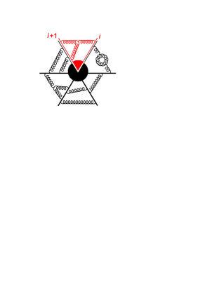
Figure 5: Infrared structure of leading-color scattering amplitudes for particles in the adjoint representation. The straight lines represent hard external states, while the curly lines carry soft or collinear virtual momenta. At leading color, soft exchanges are confined to wedges between the hard lines.

For a general theory, the Sudakov form factor at scale $Q^{2}$ can be written as MagneaSterman

$${\cal M}^{[gg\to 1]}\biggl{(}{Q^{2}\over\mu^{2}},\alpha_{s}(\mu),\epsilon\biggr{)} = \exp\Biggl{\{}{1\over 2}\int_{0}^{-Q^{2}}{d\xi^{2}\over\xi^{2}}\biggl{[}{\cal K}^{[g]}\bigl{(}\alpha_{s}(\mu),\epsilon\bigr{)}+{\cal G}^{[g]}\biggl{(}-1,\bar{\alpha}_{s}\Bigl{(}{\mu^{2}\over\xi^{2}},\alpha_{s}(\mu),\epsilon\Bigr{)},\epsilon\biggr{)}$$ (39)

$$\hskip 28.45274pt+{1\over 2}\int_{\xi^{2}}^{\mu^{2}}{d\tilde{\mu}^{2}\over\tilde{\mu}^{2}}\gamma_{K}^{[g]}\biggl{(}\bar{\alpha}_{s}\Bigl{(}{\mu^{2}\over\tilde{\mu}^{2}},\alpha_{s}(\mu),\epsilon\Bigr{)}\biggr{)}\biggr{]}\Biggr{\}}\,,$$

where $\gamma_{K}^{[g]}$ denotes the soft or (Wilson line) cusp anomalous dimension, which will produce a $1/\epsilon^{2}$ pole after integration. The function ${\cal K}^{[g]}$ is a series of counterterms (pure poles in $\epsilon$), while ${\cal G}^{[g]}$ includes non-singular dependence on $\epsilon$ before integration, and produces a $1/\epsilon$ pole after integration.

In MSYM, $\alpha_{s}(\mu)$ is a constant, and the running coupling $\bar{\alpha}_{s}(\mu^{2}/\tilde{\mu}^{2},\alpha_{s},\epsilon)$ in $4-2\epsilon$ dimensions has only trivial (engineering) dependence on the scale,

$$\bar{\alpha}_{s}\Bigl{(}{\mu^{2}\over\tilde{\mu}^{2}},\alpha_{s}(\mu),\epsilon\Bigr{)}=\alpha_{s}\times\biggl{(}{\mu^{2}\over\tilde{\mu}^{2}}\biggr{)}^{\epsilon}\Bigl{(}4\pi e^{-\gamma}\Bigr{)}^{\epsilon}\,.$$ (40)

This simple dependence makes it very easy to perform the integrals over $\xi$ and $\tilde{\mu}$.

Following refs. MagneaSterman ; StermanTY , we expand ${\cal K}^{[g]}$, $\gamma_{K}^{[g]}$, and ${\cal G}^{[g]}$ in powers of $\alpha_{s}$,

$${\cal K}^{[g]}(\alpha_{s},\epsilon) = \sum_{l=1}^{\infty}{1\over 2l\epsilon}a^{l}\,\hat{\gamma}_{K}^{(l)}\,,$$ (41)

$$\gamma_{K}^{[g]}\biggl{(}\bar{\alpha}_{s}\Bigl{(}{\mu^{2}\over\tilde{\mu}^{2}},\alpha_{s},\epsilon\Bigr{)}\biggr{)} = \sum_{l=1}^{\infty}a^{l}\Bigl{(}{\mu^{2}\over\tilde{\mu}^{2}}\Bigr{)}^{l\epsilon}\hat{\gamma}_{K}^{(l)}\,,$$ (42)

$${\cal G}^{[g]}\biggl{(}-1,\bar{\alpha}_{s}\Bigl{(}{\mu^{2}\over\xi^{2}},\alpha_{s},\epsilon\Bigr{)},\epsilon\biggr{)} = \sum_{l=1}^{\infty}a^{l}\Bigl{(}{\mu^{2}\over\xi^{2}}\Bigr{)}^{l\epsilon}{\hat{\cal G}}_{0}^{(l)}\,,$$ (43)

where $a$ is defined in eq. (25) and the hats are a reminder that the leading-$N_{c}$ dependence has also been removed in eqs. (41), (42) and (43). That is, the perturbative coefficients (defined with expansion parameter $\alpha_{s}/(2\pi)$) have a leading-color dependence on $N_{c}$ of,

$$\gamma_{K}^{(l)}=\hat{\gamma}_{K}^{(l)}\,N_{c}^{l}\,,\hskip 56.9055pt{\cal G}_{0}^{(l)}=\hat{\cal G}_{0}^{(l)}\,N_{c}^{l}\,.$$ (44)

We can suppress the $[g]$ label because the $N=4$ MHV amplitudes are all related by supersymmetry Ward identities SWI , so that the corresponding functions for external gluinos, etc., are the same as for gluons. Equation (41) follows from solving eqs. (2.12) and (2.13) of ref. MagneaSterman in the conformal case ($\beta\equiv 0$). In this case, ${\cal K}^{[g]}$ contains only single poles in $\epsilon$, which are simply related to $\gamma_{K}^{[g]}$.

The integral over ${\cal G}$ is very simple,

$$\int_{0}^{-Q^{2}}{d\xi^{2}\over\xi^{2}}{\cal G}^{[g]}=-\sum_{l=1}^{\infty}\ {a^{l}\over l\epsilon}\,\Bigl{(}{\mu^{2}\over-Q^{2}}\Bigr{)}^{l\epsilon}{\hat{\cal G}}_{0}^{(l)}\,.$$ (45)

The first integral over $\gamma_{K}$ gives,

$$\int_{\xi^{2}}^{\mu^{2}}{d\tilde{\mu}^{2}\over\tilde{\mu}^{2}}\gamma_{K}^{[g]}=\sum_{l=1}^{\infty}\ {a^{l}\over l\epsilon}\,\biggl{[}\Bigl{(}{\mu^{2}\over\xi^{2}}\Bigr{)}^{l\epsilon}-1\biggr{]}\hat{\gamma}_{K}^{(l)}\,.$$ (46)

Adding the ${\cal K}^{[g]}$ term to $1/2$ of eq. (46), using eq. (41), we see that the “$-1$” is cancelled. Then the integral over $\xi$ is properly regulated, and evaluates to

$$-{1\over 2}\sum_{l=1}^{\infty}{a^{l}\over(l\epsilon)^{2}}\Bigl{(}{\mu^{2}\over-Q^{2}}\Bigr{)}^{l\epsilon}\hat{\gamma}_{K}^{(l)}\,.$$ (47)

Combining this result with eq. (45) gives

$${\cal M}^{[gg\to 1]}\biggl{(}{Q^{2}\over\mu^{2}},\alpha_{s}(\mu),\epsilon\biggr{)}=\exp\Biggl{[}-{1\over 4}\sum_{l=1}^{\infty}a^{l}\Bigl{(}{\mu^{2}\over-Q^{2}}\Bigr{)}^{l\epsilon}\biggl{(}{\hat{\gamma}_{K}^{(l)}\over(l\epsilon)^{2}}+{2\hat{\cal G}_{0}^{(l)}\over l\epsilon}\biggr{)}\Biggr{]}\,.$$ (48)

We need eq. (48) for a neighboring pair of legs $i,i+1$ in the $n$-point amplitude, so that $Q^{2}$ should be replaced by the invariant $s_{i,i+1}$. Taking the product over all $i$, eq. (38) becomes

$${\cal M}_{n} = \exp\Biggl{[}-{1\over 8}\sum_{l=1}^{\infty}a^{l}\,\Bigl{(}\hat{\gamma}_{K}^{(l)}+2l\hat{\cal G}_{0}^{(l)}\epsilon\Bigr{)}{1\over(l\epsilon)^{2}}\sum_{i=1}^{n}\Bigl{(}{\mu^{2}\over-s_{i,i+1}}\Bigr{)}^{l\epsilon}\Biggr{]}\times h_{n}\,.$$ (49)

We may rearrange this a bit, to give

$${\cal M}_{n} = \exp\Biggl{[}\sum_{l=1}^{\infty}a^{l}\,f^{(l)}(\epsilon)\hat{I}_{n}^{(1)}(l\epsilon)\Biggr{]}\times\tilde{h}_{n}\,,$$ (50)

where $f^{(l)}(\epsilon)$ is defined in eq. (26), with the identifications,

$$f^{(l)}_{0} = {1\over 4}\,\hat{\gamma}_{K}^{(l)}\,,$$ (51)

$$f^{(l)}_{1} = {l\over 2}\,\hat{\cal G}_{0}^{(l)}\,,$$ (52)

and

$$\hat{I}_{n}^{(1)}(\epsilon)=-{1\over 2}{1\over\epsilon^{2}}\sum_{i=1}^{n}\Bigl{(}{\mu^{2}\over-s_{i,i+1}}\Bigr{)}^{\epsilon}\,.$$ (53)

Here $\tilde{h}_{n}$ differs from $h_{n}$ by a finite shift, due to the ${\cal O}(\epsilon^{2})$ terms in $f^{(l)}(\epsilon)$, which we introduce to help make contact with the exponentiated ansatz (24). Using $f^{(1)}(\epsilon)=1$ and eqs. (19) and (22), we may read off the first few loop orders,

$$\hat{\gamma}_{K}^{(1)} = 4\,,$$

$$\hat{\gamma}_{K}^{(2)} = -4\zeta_{2}\,,$$ (54)

$$\hat{\gamma}_{K}^{(3)} = 22\,\zeta_{4}\,,$$

and

$$\hat{\cal G}_{0}^{(1)} = 0\,,$$

$$\hat{\cal G}_{0}^{(2)} = -\zeta_{3}\,,$$ (55)

$$\hat{\cal G}_{0}^{(3)} = 4\zeta_{5}+{10\over 3}\zeta_{2}\zeta_{3}\,.$$

The quantity $\hat{I}_{n}^{(1)}(\epsilon)$ is a function that captures the divergences of the planar one-loop $n$-point amplitudes in MSYM IROneLoop , after extracting the leading-$N_{c}$ dependence as in ref. TwoLoopSplitting . The $\hat{I}_{n}^{(1)}$ defined in eq. (8.9) of ref. TwoLoopSplitting contained a prefactor of $e^{-\epsilon\psi(1)}/\Gamma(1-\epsilon)$, following conventions of Catani CataniIR . Here we adopt a convention closer to that of Sterman and Tejeda-Yeomans StermanTY , without such a prefactor. The difference between eq. (8.9) of ref. TwoLoopSplitting and eq. (53) above is a finite quantity, because $e^{-\epsilon\psi(1)}/\Gamma(1-\epsilon)=1+{\cal O}(\epsilon^{2})$. Finite remainders will differ between the two conventions.

Starting from eq. (50), and using the fact that the difference between $M_{n}^{(1)}(l\epsilon)$ and $\hat{I}_{n}^{(1)}(l\epsilon)$ is finite, we can reshuffle the finite terms once more to obtain,

$${\cal M}_{n}=\exp\Biggl{[}\sum_{l=1}^{\infty}a^{l}\,\Bigl{(}f^{(l)}(\epsilon)M_{n}^{(1)}(l\epsilon)+h_{n}^{(l)}(\epsilon)\Bigr{)}\Biggr{]}\,.$$ (56)

We have moved the hard function into the exponent without loss of generality, because we allow for a new function $h_{n}^{(l)}$ at each order $l$.

Finally we compare the exponentiated ansatz (24) with the exponentiation of the IR divergences (56). We see that they agree if we identify

$$h_{n}^{(l)}(k_{i},\epsilon)=C^{(l)}+E_{n}^{(l)}(\epsilon)\,.$$ (57)

In some sense, the content of the iterative structure of planar MSYM, beyond the level of consistency with IR resummation, is that the (suitably-defined) exponentiated hard remainders $h_{n}^{(l)}(k_{i},\epsilon)$ approach constants, independent of the kinematics and of $n$, as $\epsilon\to 0$, since $E_{n}^{(l)}(\epsilon)$ is of ${\cal O}(\epsilon)$.

IV.3 Finite Remainders

Next we shall obtain iterative formulae for two series of functions: the $\hat{I}_{n}^{(L)}$ governing IR divergences for the $L$-loop $n$-point planar amplitudes, and the $F_{n}^{(L)}$ representing the finite remainders of the amplitudes, after subtracting these divergences. The formulae will be very similar in form to the full amplitude relation (30).

Following the structure uncovered explicitly at one, two, and three loops IROneLoop ; CataniIR ; StermanTY , we define the finite remainder for the $L$-loop amplitude by writing

$$M_{n}^{(L)}(\epsilon)=\sum_{l=0}^{L-1}\hat{I}_{n}^{(L-l)}(\epsilon)\,M_{n}^{(l)}(\epsilon)+F_{n}^{(L)}(\epsilon)\,,$$ (58)

or

$$F_{n}^{(L)}(\epsilon)=M_{n}^{(L)}-\sum_{l=0}^{L-1}\hat{I}_{n}^{(L-l)}\,M_{n}^{(l)}\,,$$ (59)

where $M_{n}^{(0)}\equiv 1$. We insert the iteration formula (30) for the first term, $M_{n}^{(L)}$, on the right-hand side of eq. (59). We split $M_{n}^{(1)}(L\epsilon)\to\hat{I}_{n}^{(1)}(L\epsilon)+F_{n}^{(1)}(L\epsilon)$ in this formula. For the lower-loop amplitudes, $M_{n}^{(l)}$, we recursively substitute in the finite-remainder formula for smaller values of $l$,

$$M_{n}^{(l)}=\sum_{k=0}^{l-1}\hat{I}_{n}^{(l-k)}M_{n}^{(k)}+F_{n}^{(l)}\,.$$ (60)

At this point, the expression for $F_{n}^{(L)}(\epsilon)$ is a polynomial in $\hat{I}_{n}^{(l)}$ and $F_{n}^{(l)}$, which has the special property that there are no mixed $\hat{I}$-$F$ terms. (If there had been such terms, it would have signaled an inconsistency.) We can remove the pure-$\hat{I}$ terms by choosing $\hat{I}_{n}^{(L)}$ to cancel them. The resulting finite expression gives $F_{n}^{(L)}(\epsilon)$ as a polynomial in the lower-loop $F_{n}^{(l)}(\epsilon)$.

We find that the solutions for $\hat{I}_{n}^{(L)}(\epsilon)$ and $F_{n}^{(L)}(\epsilon)$ are expressible in terms of the same function $X_{n}^{(L)}$ defined in eq. (34), but where the role of $M_{n}$ is played instead by $-\hat{I}_{n}$ and $F_{n}$, respectively:

$$\hat{I}_{n}^{(L)}(\epsilon) = -X_{n}^{(L)}\bigl{[}-\hat{I}_{n}^{(l)}(\epsilon)]+f^{(L)}(\epsilon)\hat{I}_{n}^{(1)}(L\epsilon)\,,$$ (61)

$$F_{n}^{(L)}(\epsilon) = X_{n}^{(L)}\bigl{[}F_{n}^{(l)}(\epsilon)]+f^{(L)}(\epsilon)F_{n}^{(1)}(L\epsilon)+C^{(L)}+E_{n}^{(L)}(\epsilon)\,.$$ (62)

The Taylor expansion (34) can be used to evaluate eqs. (61) and (62) to any desired loop order.

Because the form of eq. (62) for $F_{n}^{(L)}(\epsilon)$ is completely analogous to the iteration formula (30) for the full amplitude $M_{n}^{(L)}(\epsilon)$, we see that the finite remainders can be exponentiated as,

$${\cal F}_{n}(\epsilon)\equiv 1+\sum_{L=1}^{\infty}a^{L}F_{n}^{(L)}(\epsilon)=\exp\Biggl{[}\sum_{l=1}^{\infty}a^{l}\Bigl{(}f^{(l)}(\epsilon)F_{n}^{(1)}(l\epsilon)+C^{(l)}+E_{n}^{(l)}(\epsilon)\Bigr{)}\Biggr{]}\,.$$ (63)

Letting $\epsilon\to 0$, we have

$${\cal F}_{n}(0)\equiv 1+\sum_{L=1}^{\infty}a^{L}F_{n}^{(L)}(0)=\exp\Biggl{[}\sum_{l=1}^{\infty}a^{l}\Bigl{(}f^{(l)}_{0}F_{n}^{(1)}(0)+C^{(l)}\Bigr{)}\Biggr{]}\,,$$ (64)

where

$$f^{(l)}_{0}\equiv f^{(l)}(0)\,.$$ (65)

Using eq. (51) we may then rewrite this as,

$${\cal F}_{n}(0)=\exp\Biggl{[}{1\over 4}\gamma_{K}F_{n}^{(1)}(0)+C\Biggr{]}\,.$$ (66)

The soft anomalous dimension is

$$\gamma_{K} = \sum_{l=1}^{\infty}\hat{\gamma}_{K}^{(l)}a^{l}=4\,a-4\zeta_{2}\,a^{2}+22\zeta_{4}\,a^{3}+\cdots\,,$$ (67)

where we used eq. (54). Similarly, from eqs. (20), (23) and (27), we have,

$$C = \sum_{l=1}^{\infty}C^{(l)}a^{l}=-{1\over 2}\zeta_{2}^{2}\,a^{2}+\Biggl{[}\biggl{(}{341\over 216}\,+{2\over 9}c_{1}\biggl{)}\zeta_{6}+\biggl{(}-{17\over 9}+{2\over 9}c_{2}\biggr{)}\zeta_{3}^{2}\Biggr{]}\,a^{3}+\cdots\,.$$ (68)

As mentioned below eq. (23), the rational numbers $c_{1}$ and $c_{2}$ are yet to be determined. The resummation (66) of the finite remainders of the MHV amplitudes, as a consequence of the exponentiated ansatz (24), is one of the key results of this paper.

For the $F_{n}^{(l)}(0)$, the argument $l\epsilon$ in eq. (62) has disappeared as $\epsilon\to 0$. Hence we can recursively substitute back to obtain formulas solely in terms of $F_{n}^{(1)}(0)$. Equivalently, we can series expand the exponential in eq. (64) or (66). The first few values are,

$$F_{n}^{(2)}(0) = {1\over 2}\Bigl{(}F_{n}^{(1)}(0)\Bigr{)}^{2}+f^{(2)}_{0}F_{n}^{(1)}(0)+C^{(2)}\,,$$ (69)

$$F_{n}^{(3)}(0) = -{1\over 3}\Bigl{(}F_{n}^{(1)}(0)\Bigr{)}^{3}+F_{n}^{(1)}(0)F_{n}^{(2)}(0)+f^{(3)}_{0}F_{n}^{(1)}(0)+C^{(3)}$$ (70)

$$= {1\over 6}\Bigl{(}F_{n}^{(1)}(0)\Bigr{)}^{3}+f^{(2)}_{0}\Bigl{(}F_{n}^{(1)}(0)\Bigr{)}^{2}+\Bigl{(}f^{(3)}_{0}+C^{(2)}\Bigr{)}F_{n}^{(1)}(0)+C^{(3)}\,,$$ (71)

$$F_{n}^{(4)}(0) = {1\over 4}\Bigl{(}F_{n}^{(1)}(0)\Bigr{)}^{4}-\Bigl{(}F_{n}^{(1)}(0)\Bigr{)}^{2}F_{n}^{(2)}(0)+F_{n}^{(1)}(0)F_{n}^{(3)}(0)+{1\over 2}\Bigl{(}F_{n}^{(2)}(0)\Bigr{)}^{2}$$ (73)

$$\hskip 1.42271pt+f^{(4)}_{0}F_{n}^{(1)}(0)+C^{(4)}$$

$$= {1\over 24}\Bigl{(}F_{n}^{(1)}(0)\Bigr{)}^{4}+{1\over 2}f^{(2)}_{0}\Bigl{(}F_{n}^{(1)}(0)\Bigr{)}^{3}+{1\over 2}\Bigl{(}[f^{(2)}_{0}]^{2}+2f^{(3)}_{0}+C^{(2)}\Bigr{)}\Bigl{(}F_{n}^{(1)}(0)\Bigr{)}^{2}$$

$$\hskip 1.42271pt+\Bigl{(}f^{(4)}_{0}+f^{(2)}_{0}C^{(2)}+C^{(3)}\Bigr{)}F_{n}^{(1)}(0)+C^{(4)}+{1\over 2}[C^{(2)}]^{2}\,.$$

Thus, starting from the ansatz (24), we have succeeded in expressing the $n$-point $L$-loop MHV finite remainders directly in terms of the one-loop finite remainders.

We remark that the two-loop result (69) differs slightly (in the constant term) from the corresponding eq. (16) for $n=4$ in ref. Iterate2 . The reason is that the definition of the two-loop divergence used there, interpreted in terms of $\hat{I}_{n}^{(2)}$, does not obey eq. (61) for $L=2$, but differs from that $\hat{I}_{n}^{(2)}$ by a finite (${\cal O}(\epsilon^{0})$) amount. The definition we use here is more convenient because of its simple generalization to higher loops.

The one-loop finite remainders $F_{n}^{(1)}(0)$ for the MHV amplitudes in MSYM were evaluated for all $n$ in ref. NeqFourOneLoop , using the unitarity method. Modifying those results to the conventions of this paper, the finite terms are explicitly, for all $n\geq 5$,

$$F_{n}^{(1)}(0)={1\over 2}\sum_{i=1}^{n}g_{n,i}\,,$$ (74)

where

$$g_{n,i} = -\sum_{r=2}^{\lfloor n/2\rfloor-1}\ln\Biggl{(}{-t^{[r]}_{i}\over-t^{[r+1]}_{i}}\Biggr{)}\ln\Biggl{(}{-t^{[r]}_{i+1}\over-t^{[r+1]}_{i}}\Biggr{)}+D_{n,i}+L_{n,i}+{3\over 2}\zeta_{2}\,,$$ (75)

and where $\lfloor x\rfloor$ is the greatest integer less than or equal to $x$. Here $t^{[r]}_{i}=(k_{i}+\cdots+k_{i+r-1})^{2}$ are the momentum invariants, so that $t^{[1]}_{i}=0$ and $t^{[2]}_{i}=s_{i,i+1}$. (All indices are understood to be $\mathop{\rm mod}\nolimits n$.) The form of $D_{n,i}$ and $L_{n,i}$ depends upon whether $n$ is odd or even. For $n=2m+1$,

$$D_{2m+1,i} = -\sum_{r=2}^{m-1}{\mathop{\rm Li}\nolimits}_{2}\Biggl{(}1-{t^{[r]}_{i}t^{[r+2]}_{i-1}\over t^{[r+1]}_{i}t^{[r+1]}_{i-1}}\Biggr{)}\,,$$ (76)

$$L_{2m+1,i} = -{1\over 2}\ln\Biggl{(}{-t^{[m]}_{i}\over-t^{[m]}_{i+m+1}}\Biggr{)}\ln\Biggl{(}{-t^{[m]}_{i+1}\over-t^{[m]}_{i+m}}\Biggr{)}\,,$$ (77)

whereas for $n=2m$,

$$D_{2m,i} = -\sum_{r=2}^{m-2}{\mathop{\rm Li}\nolimits}_{2}\Biggl{(}1-{t^{[r]}_{i}t^{[r+2]}_{i-1}\over t^{[r+1]}_{i}t^{[r+1]}_{i-1}}\Biggr{)}-{1\over 2}{\mathop{\rm Li}\nolimits}_{2}\Biggl{(}1-{t^{[m-1]}_{i}t^{[m+1]}_{i-1}\over t^{[m]}_{i}t^{[m]}_{i-1}}\Biggr{)}\,,$$ (78)

$$L_{2m,i} = -{1\over 4}\ln\Biggl{(}{-t^{[m]}_{i}\over-t^{[m]}_{i+m+1}}\Biggr{)}\ln\Biggl{(}{-t^{[m]}_{i+1}\over-t^{[m]}_{i+m}}\Biggr{)}\,.$$ (79)

For $n=4$ the above formula does not hold, but the finite remainder is simply,

$$F_{4}^{(1)}(0)={1\over 2}\ln^{2}\biggl{(}{-t\over-s}\biggr{)}+4\zeta_{2}\,.$$ (80)

Assuming that the exponentiated ansatz (24) holds, then the exponentiated finite remainders ${\cal F}_{n}(0)$ given in eq. (66) are completely determined to all loop orders, in terms of the one-loop remainders $F_{n}^{(1)}(0)$ just presented, plus the series of constants $\gamma_{K}$ and $C$ given in eqs. (67) and (68).

V Collinear behavior and consistency of all-$n$ ansatz

In this section we discuss the consistency of the $n$-point iterative ansatz (30) with the behavior of amplitudes under factorization. In a supersymmetric theory, MHV amplitudes have no multi-particle poles; the residues vanish by a supersymmetry Ward identity SWI . This property is manifest in our ansatz, because neither the tree amplitude $A_{n}^{{(0)},\,{\rm MHV}}(1,2,\ldots,n)$ nor the one-loop amplitude $M_{n-1}^{(1)}(l\epsilon)$ contain such poles. Hence only factorizations as pairs of momenta become collinear need to be analyzed.

In general, color-ordered amplitudes $A_{n}^{(L)}(1,2,\ldots,n)$ satisfy simple properties as the momenta of two color-adjacent legs $k_{i}$, $k_{i+1}$ become collinear, TreeReview ; NeqFourOneLoop ; OneLoopSplitting ; KosowerSplit ; OneLoopReview ,

$$A_{n}^{(L)}(\ldots,i^{\lambda_{i}},(i+1)^{\lambda_{i+1}},\ldots)\,\longrightarrow\sum_{l=0}^{L}\sum_{\lambda=\pm}\mathop{\rm Split}\nolimits^{(l)}_{-\lambda}(z;i^{\lambda_{i}}\kern-1.0pt,(i+1)^{\lambda_{i+1}})A_{n-1}^{(L-l)}(\ldots,P^{\lambda}\kern-5.0pt,\ldots)\,.\hskip 28.45274pt$$ (81)

The index $l$ sums over the different loop orders of contributing splitting amplitudes $\mathop{\rm Split}\nolimits_{-\lambda}^{(l)}$, while $\lambda$ sums over the helicities of the intermediate leg $k_{P}=-(k_{i}+k_{i+1})$, and $z$ is the longitudinal momentum fraction of $k_{i}$, $k_{i}\approx-zk_{P}$. The splitting amplitudes are universal and gauge invariant.

The tree-level splitting amplitudes $\mathop{\rm Split}\nolimits_{-\lambda}^{(0)}$ are the same in MSYM as in QCD. At loop level, the MSYM splitting amplitudes are all proportional to the tree-level ones. The proportionality factors depend only on $z$ and $\epsilon$, not on the helicity configuration, nor (except for a trivial dimensional factor) on kinematic invariants NeqFourOneLoop . It is thus convenient to write the $L$-loop planar splitting amplitudes in terms of “renormalization” factors $r_{S}^{(L)}(\epsilon;z,s)$, defined by

$$\mathop{\rm Split}\nolimits_{-\lambda_{P}}^{(L)}(1^{\lambda_{1}},2^{\lambda_{2}}) = \,r_{S}^{(L)}(\epsilon;z,s)\mathop{\rm Split}\nolimits_{-\lambda_{P}}^{(0)}(1^{\lambda_{1}},2^{\lambda_{2}})\,,$$ (82)

where $s=(k_{1}+k_{2})^{2}$.

Using eqs. (81) and (82), we see that the amplitude ratios $M_{n}^{(L)}(\epsilon)\equiv A_{n}^{(L)}/A_{n}^{(0)}$ behave in collinear limits as,

$$M_{n}^{{(1)}}(\epsilon) \rightarrow M_{n-1}^{{(1)}}(\epsilon)+r_{S}^{{(1)}}(\epsilon)\,,$$ (83)

$$M_{n}^{{(2)}}(\epsilon) \rightarrow M_{n-1}^{{(2)}}(\epsilon)+r_{S}^{{(1)}}(\epsilon)M_{n-1}^{{(1)}}(\epsilon)+r_{S}^{(2)}(\epsilon)\,,$$ (84)

or at three loops,

$$M_{n}^{{(3)}}(\epsilon) \rightarrow M_{n-1}^{{(3)}}(\epsilon)+r_{S}^{{(1)}}(\epsilon)M_{n-1}^{{(2)}}(\epsilon)+r_{S}^{{(2)}}(\epsilon)M_{n-1}^{{(1)}}(\epsilon)+r_{S}^{{(3)}}(\epsilon)\,,$$ (85)

where $r_{S}^{(0)}(\epsilon)\equiv 1$ and we have suppressed all functional arguments except for $\epsilon$.

The one-loop splitting amplitudes in MSYM have been calculated to all orders in $\epsilon$, with the result OneLoopSplitting ,

$$r_{S}^{{(1)}}(\epsilon;z,s) = {\hat{c}_{\Gamma}\over\epsilon^{2}}\biggl{(}{\mu^{2}\over-s}\biggr{)}^{\epsilon}\biggl{[}-{\pi\epsilon\over\sin(\pi\epsilon)}\biggl{(}{1-z\over z}\biggr{)}^{\epsilon}+2\,\sum_{k=0}^{\infty}\epsilon^{2k+1}\,\mathop{\rm Li}\nolimits_{2k+1}\biggl{(}{-z\over 1-z}\biggr{)}\biggr{]}\,,$$ (86)

where $\mathop{\rm Li}\nolimits_{n}$ is the $n$-th polylogarithm (defined in eq. (105)), and

$$\hat{c}_{\Gamma}={e^{\epsilon\gamma}\over 2}{\Gamma(1+\epsilon)\Gamma^{2}(1-\epsilon)\over\Gamma(1-2\epsilon)}\,.$$ (87)

In refs. Iterate2 ; TwoLoopSplitting , the two-loop splitting amplitudes in MSYM were computed through ${\cal O}(\epsilon^{0})$ using the unitarity method as described in ref. KosowerSplit . The result of this computation is a very simple formula, expressing the two-loop splitting amplitude in terms of the one-loop one,

$$r^{(2)}_{S}(\epsilon;z,s)={1\over 2}\Bigl{(}r^{(1)}_{S}(\epsilon;z,s)\Bigr{)}^{2}+f^{(2)}(\epsilon)\,r^{(1)}_{S}(2\epsilon;z,s)+{\cal O}(\epsilon)\,,$$ (88)

where $f^{(2)}(\epsilon)$ is given in eq. (19). (This result was actually obtained before the iterative relation (18), and motivated its discovery.)

The consistency of the $n$-point ansatz (30) for $L=2$ (with $X_{n}^{(2)}$ given by eq. (31)) may be easily confirmed using these splitting functions Iterate2 . Inserting the collinear behavior of the one-loop amplitudes (83) into the right-hand side, we obtain,

$$M_{n}^{(2)}(\epsilon) \rightarrow {1\over 2}\Bigl{(}M_{n-1}^{{(1)}}(\epsilon)+r_{S}^{{(1)}}(\epsilon)\Bigr{)}^{2}+f^{(2)}(\epsilon)\,(M_{n-1}^{{(1)}}(2\epsilon)+r_{S}^{{(1)}}(2\epsilon))-{1\over 2}\zeta_{2}^{2}$$ (89)

$$= M_{n-1}^{(2)}(\epsilon)+r_{S}^{{(1)}}(\epsilon)M_{n-1}^{(1)}(\epsilon)+r_{S}^{{(2)}}(\epsilon)\,,$$

where we used eqs. (30) and (88) to rearrange the expression into the required form (84) for correct two-loop collinear behavior. Since there are no multi-particle poles in the MHV case, eq. (89) confirms that the ansatz (30) has the correct factorization properties in all channels at two loops.

Similarly, we can require that the ansatz (30) is consistent with collinear factorization beyond two loops, and thereby obtain an iterative ansatz for the planar $L$-loop splitting amplitudes in MSYM. For $L=3$, the ansatz reads,

$$M_{n}^{(3)}(\epsilon) = -{1\over 3}\Bigl{[}M_{n}^{(1)}(\epsilon)\Bigr{]}^{3}+M_{n}^{(1)}(\epsilon)\,M_{n}^{(2)}(\epsilon)+f^{(3)}(\epsilon)\,M_{n}^{(1)}(3\,\epsilon)+C^{(3)}+{\cal O}(\epsilon)\,.$$ (90)

If we insert the properties of one- and two-loop amplitudes (83) and (84) into the collinear limit of the right-hand side of eq. (90), we obtain,

$$M_{n}^{(3)}(\epsilon) \rightarrow -{1\over 3}\Bigl{[}M_{n-1}^{(1)}(\epsilon)+r_{S}^{{(1)}}(\epsilon)\Bigr{]}^{3}$$ (91)

$$\hbox{}+\Bigl{(}M_{n-1}^{(1)}(\epsilon)+r_{S}^{{(1)}}(\epsilon)\Bigr{)}\,\Bigl{(}M_{n-1}^{{(2)}}(\epsilon)+r_{S}^{{(1)}}(\epsilon)M_{n-1}^{{(1)}}(\epsilon)+r_{S}^{{(2)}}(\epsilon)\Bigr{)}$$

$$\hbox{}+f^{(3)}(\epsilon)\,\Bigl{(}M_{n-1}^{(1)}(3\,\epsilon)+r_{S}^{(1)}(3\,\epsilon)\Bigr{)}+C^{(3)}+{\cal O}(\epsilon)\,.$$

After rearranging terms, we can get consistency with eq. (85), provided that the three-loop splitting function obeys,

$$r^{(3)}_{S}(\epsilon)=-{1\over 3}\Bigl{(}r^{(1)}_{S}(\epsilon)\Bigr{)}^{3}+r^{(1)}_{S}(\epsilon)r^{(2)}_{S}(\epsilon)+f^{(3)}(\epsilon)\,r^{(1)}_{S}(3\epsilon)+{\cal O}(\epsilon)\,.$$ (92)

By repeating this exercise at $L$ loops, and collecting the terms that are independent of $M_{n-1}^{(l)}$, we see that the relation,

$$r_{S}^{(L)}(\epsilon)=X^{(L)}\bigl{[}r^{(l)}_{S}(\epsilon)\bigr{]}+f^{(L)}(\epsilon)\,r_{S}^{(L)}(L\epsilon)+{\cal O}(\epsilon)\,,$$ (93)

is the one required for consistency. (We have dropped the subscript $n$ from $X_{n}^{(L)}$ because it is out of place here, but it is the same function of lower-loop quantities defined in eq. (34).) In other words, the $L$-loop splitting amplitude functions $r_{S}^{(L)}$ obey exactly the same type of iterative relation as the scattering amplitudes $M_{n}^{(L)}$, but without the “inhomogeneous” constant terms $C^{(L)}$. Because the one-loop splitting amplitude $r_{S}^{(1)}(L\epsilon)$ begins at order ${\cal O}(\epsilon^{-2})$, the relation (93) allows the ${\cal O}(\epsilon^{2})$ coefficient of $f^{(L)}(\epsilon)$, namely $f_{2}^{(L)}$, to be extracted from the ${\cal O}(\epsilon^{0})$ term in the $L$-loop splitting amplitude.

VI Anomalous dimensions and Sudakov form factors

The soft anomalous dimension $\gamma_{K}$ controlling the $1/\epsilon^{2}$ IR singularities of the loop amplitudes arises from an edge of phase space, the Sudakov region, where a hard line can only emit soft gluons. In the loop amplitudes these gluons are virtual, of course, but they are related to real soft-gluon emission by the cancellation of infrared poles in infrared-safe cross sections for Sudakov-type processes Sudakov ; SoftGluonSummation . For example, the splitting kernel $P_{ii}(x)$ describes the probability for a parton $i$ to split collinearly into a parton of the same species $i$, plus anything else, where the second parton $i$ retains a fraction $x$ of the longitudinal momentum of the first parton $i$. In the limit $x\to 1$, this splitting kernel is dominated by soft-gluon emission, and has the form,

$$P_{ii}(x)\to{A(\alpha_{s})\over(1-x)_{+}}+B(\alpha_{s})\delta(1-x)+\ldots,\qquad{\rm as}\ \ x\to 1,$$ (94)

where $A(\alpha_{s})$ is related KM to the soft (cusp) anomalous dimension by,

$$A(\alpha_{s})={1\over 2}\,\gamma_{K}(\alpha_{s})\,.$$ (95)

The splitting kernel is related by a Mellin transform to the anomalous dimensions of leading-twist operators of spin $j$,

$$\gamma(j)\equiv-\int_{0}^{1}dx\,x^{j-1}P(x).$$ (96)

Thus the soft anomalous dimension also controls the large-spin behavior of these anomalous dimensions LeadingN ,

$$\gamma(j)={1\over 2}\gamma_{K}(\alpha_{s})\ (\ln(j)+\gamma_{e})-B(\alpha_{s})+{\cal O}(\ln(j)/j)\,,$$ (97)

where here we take $\gamma_{e}$ as Euler’s constant.

KLOV KLOV have made a very interesting observation: the anomalous dimensions of MSYM may be extracted directly from the corresponding anomalous dimensions of QCD MVV , by keeping terms of highest “transcendentality”. Recall that for the case of the soft anomalous dimensions (large $j$ limit), the transcendentality weight is simply $n$ for $\zeta_{n}$. (Although the QCD anomalous dimensions are computed in the $\overline{\rm MS}$ regularization scheme, whereas for MSYM the DR Siegel or FDH FDH schemes are needed to preserve supersymmetry, the scheme-dependent terms drop out because they are of lower transcendentality.) Although there is no proof of KLOV’s prescription for extracting the MSYM anomalous dimensions from QCD, there are good reasons to believe that it is true KLOV ; TwoLoopSplitting .

Here we provide further evidence for the prescription, by confirming the large-spin behavior of the leading-twist anomalous dimension. We compare the KLOV result, given in eqs. (18)-(20) of ref. KLOV , against our evaluation of the same quantity from the IR divergences of the three-loop four-point amplitude. Note that their normalization convention for anomalous dimensions has an opposite overall sign from ours (which follows ref. MVV ). Also taking into account factors of 2 from the different $\alpha_{s}$ expansion parameter, and from eq. (97), we obtain from eqs. (18)-(20) of ref. KLOV ,

$$\gamma_{K}^{(1)} = 4\,N_{c}\,,$$

$$\gamma_{K}^{(2)} = -4\zeta_{2}\,N_{c}^{2}\,,$$ (98)

$$\gamma_{K}^{(3)} = 22\,\zeta_{4}\,N_{c}^{3}\,,$$

which agrees perfectly with our results (44) and (54).

We remark that the strong-coupling, large-$N_{c}$ limit of the soft anomalous dimension $\gamma_{K}$ has been obtained, using the AdS/CFT correspondence and classical supergravity methods StrongCoupling . An approximate formula interpolating between the weak and strong-coupling limits has also been constructed KLV ; KLOV .

The coefficient ${\cal G}_{0}^{(l)}$, which controls the $1/\epsilon$ singularity, may be extracted EynckLaenenMagnea from a fixed-order computation of the form factor at $l$ loops. For example, the two-loop quark form factor in QCD was computed in ref. SudakovFormFactors . From eqs. (21)–(22) of ref. StermanTY , if we follow the KLOV procedure and keep the maximal transcendentality terms ($\zeta_{3}$ at two loops) in order to convert the QCD results into MSYM results, we have,

$${\cal G}_{0}^{(1)} = 0\,,$$

$${\cal G}_{0}^{(2)} = -\zeta_{3}\,N_{c}^{2}\,.$$ (99)

We have multiplied ${\cal G}_{0}^{(2)}$ in eq. (22) of ref. StermanTY by a factor of 4 to account for the different normalization conventions used here. These results agree with our eqs. (44) and (55). Although the QCD form factors have not yet been computed at three loops, we may use our results, together with the observation of KLOV, to predict the leading-transcendentality contributions for QCD,

$${\cal G}_{0}^{(3)}=\biggl{(}4\zeta_{5}+{10\over 3}\zeta_{2}\zeta_{3}\biggr{)}N_{c}^{3}\,,$$ (100)

after the group theory Casimirs have been set to the values $C_{F}=C_{A}=N_{c}$. (At three loops, no other Casimirs can appear, so there are no subleading-color corrections to this leading-transcendentality prediction.)

VII Conclusions and outlook

In this paper we have provided strong evidence supporting the conjecture Iterate2 that the planar contributions to the scattering amplitudes of MSYM possess an iterative structure. This result is in line with the growing body of evidence that gauge theory amplitudes in general, and those of MSYM in particular, have a much simpler structure than had been anticipated.

Our evidence of iteration is based on a direct evaluation of the planar three-loop four-point amplitude of MSYM. The loop integrands for this amplitude were obtained BRY ; BDDPR using the unitarity method NeqFourOneLoop ; Fusing ; UnitarityMachinery ; OneLoopReview ; TwoLoopSplitting . This method ensures that simple structures uncovered at lower loop orders (including tree level) in turn feed into higher loops. (It also underlies much of the recent progress at one loop NewOneloop .) In order to evaluate the required three-loop integrals, we made use of important recent advances in multi-loop integration SmirnovDoubleBox ; SmirnovVeretin ; LoopIntegrationAdvance ; SmirnovTripleBox . The integrals are expressed in terms of well-studied harmonic polylogarithms HPL ; HPL2 , making it straightforward to confirm the three-loop iteration. A rather intricate set of cancellations is required, amongst the harmonic polylogarithms, and between different loop integral types contributing to the amplitudes.

Using our explicitly computed four-point amplitudes as a springboard, the known structure of infrared singularities to all loop orders MagneaSterman ; StermanTY , and the required factorization properties of amplitudes, we constructed the ansatz for the resummed $n$-point all-loop MHV amplitudes given in eq. (24). After subtracting the IR divergences, the all-loop finite remainders (66) are given in terms of known one-loop $n$-point finite remainders, as well as two coefficients, one of which is the large-spin limit of the leading-twist anomalous dimensions.

Very interestingly, the same set of leading-twist anomalous dimensions has recently been linked to integrability of MSYM by Beisert, Kristjansen and Staudacher MoreIntegrable ; Staudacher . With the assumption of integrability, Staudacher Staudacher has reproduced the leading-twist anomalous dimensions at three loops for spin $j$ up to 8. These anomalous dimensions were previously obtained by Kotikov, Lipatov, Onishchenko and Velizhanin KLOV from the QCD results of Moch, Vermaseren and Vogt MVV . (Quite recently, Staudacher’s Bethe ansatz analysis has been extended to extremely high spins, the region relevant here, confirming the prediction of KLOV for even values of $j$ up to 70 StaudacherPrivate .) If one were able to push this method to higher loop orders, and arbitrarily large spins, it would give very directly the soft anomalous dimensions appearing in our all-loop exponentiation of the MHV scattering amplitudes.

Besides confirming the iterative structure of the scattering amplitudes, our paper provides non-trivial confirmation of the form of the three-loop divergences predicted by Sterman and Tejeda-Yeomans StermanTY . It also provides supporting evidence for a number of ansätze appearing in a variety of papers. In particular, we confirm, in the high spin limit, the inspired ansätze of KLOV, and (via KLOV) of Beisert, Kristjansen and Staudacher, for obtaining the leading-twist anomalous dimensions in MSYM. By making use of KLOV’s link to QCD, via the degree of transcendentality, our work also checks indirectly a small piece of the three-loop splitting kernels in QCD, or equivalently the anomalous dimensions of leading-twist operators, computed by Moch, Vermaseren and Vogt MVV . The integrand BRY ; BDDPR used in the computation of the planar three-loop four-point amplitude has not been completely proven, but the match between its IR singularities and the formulae of Sterman and Tejeda-Yeomans, plus the demonstration of its iterative structure through the finite terms as $\epsilon\to 0$, leaves little doubt as to its veracity.

The properties found here and in ref. Iterate2 bring up the possibility that the entire perturbative series of planar MSYM is tractable. The apparent simple structure of the MHV all-loop amplitudes suggests that a loop-level twistor string interpretation will be found WittenTopologicalString ; BerkovitsWitten . It would be important to first identify the precise symmetry responsible for this structure. A more complete understanding of the iterative structure of the amplitudes should lead to important insights into quantum field theory and the AdS/CFT correspondence.

Note added

Since the first version of this paper came out, an interesting paper has appeared BC , containing a technique for computing large classes of terms for multi-loop MSYM amplitudes with many external legs, which may shed further light on the iterative relations discussed here. Also, the prediction (100) for the leading-transcendentality terms in ${\cal G}_{0}^{(3)}$ for QCD has now been confirmed ThreeLoopQCDFormFactor .

Appendix A Harmonic polylogarithms

We express the amplitudes in terms of harmonic polylogarithms HPL , which are generalizations of ordinary polylogarithms Lewin . Here we briefly summarize some salient properties. A more complete discussion is given in ref. HPL . Recipes for numerically evaluating harmonic polylogarithms may be found in ref. HPL2 .

The weight $n$ harmonic polylogarithms $H_{a_{1}a_{2}\ldots a_{n}}(x)\equiv H(a_{1},a_{2},\ldots,a_{n};x)$, with $a_{i}\in\{1,0,-1\}$, are defined recursively by,

$$H_{a_{1}a_{2}\ldots a_{n}}(x)=\int_{0}^{x}\mbox{d}t\,f_{a_{1}}(t)H_{a_{2}\ldots a_{n}}(t)\,,$$ (101)

where

$$f_{\pm 1}(x) = {1\over 1\mp x}\,,\qquad f_{0}(x)={1\over x}\,,$$ (102)

$$H_{\pm 1}(x) = \mp\ln(1\mp x)\,,\qquad H_{0}(x)=\ln x\,,$$ (103)

and at least one of the indices $a_{i}$ is non-zero. For all $a_{i}=0$, one has

$$H_{0,0,\ldots,0}(x)=\frac{1}{n!}\ln^{n}x\;.$$ (104)

If a given harmonic polylogarithm involves only parameters $a_{i}=0$ and $1$, and the number of these parameters (the weight) is less than or equal to four, it can be expressed HPL in terms of the standard polylogarithms Lewin ,

$$\mathop{\rm Li}\nolimits_{n}(z) = \sum_{j=1}^{\infty}{z^{j}\over j^{n}}=\int_{0}^{z}{\mbox{d}t\over t}\mathop{\rm Li}\nolimits_{n-1}(t)\,,$$

$$\mathop{\rm Li}\nolimits_{2}(z) = -\int_{0}^{z}{\mbox{d}t\over t}\ln(1-t)\,,$$ (105)

with $n=2,3,4$, and where $z$ may take the values $x$, $1/(1-x)$, or $-x/(1-x)$. (For $n<4$, not all of these values are required, due to identities.) Here we need only $a_{i}\in\{0,1\}$, but weights up to six. In the Euclidean region for the planar four-point process, namely $s<0$, $t<0$, $u>0$, with the identification $x=-t/s$, the argument $x$ of the harmonic polylogarithms will be negative.

The harmonic polylogarithms are not all independent; they are related by sets of identities HPL . One set of identities, derived using integration by parts,

$$H_{a_{1}a_{2}\ldots a_{p}0}(x)=\ln x\,H_{a_{1}a_{2}\ldots a_{p}}(x)-H_{0a_{1}a_{2}\ldots a_{p}}(x)-H_{a_{1}0a_{2}\ldots a_{p}}(x)-\cdots-H_{a_{1}a_{2}\ldots 0a_{p}}(x)\,,$$ (106)

allows one to remove trailing zeroes from the string of parameters $a_{i}$. The remaining $H_{a_{1}a_{2}\ldots a_{n}}(x)$ with $a_{n}=1$ are well-behaved as $x\to 0$; in fact they all vanish there.

Because the integrals appear in the MSYM amplitudes with arguments $(s,t)$ and $(t,s)$, we need a set of identities relating harmonic polylogarithms with argument $x=-t/s$ to those with argument $y=-s/t=1/x$. As explained in ref. HPL (see the discussion near eqs. (55) of that reference), we may construct the required set of identities by induction on the weight of the harmonic polylogarithms. For the first few weights, in the region $-1\geq x\geq 0$, and letting $L=\ln(s/t)=\ln(-1/x)$, we have, for example,

$$H_{1}(y) = H_{1}(x)-L\,,$$

$$H_{0,1}(y) = -H_{0,1}(x)-{1\over 2}L^{2}-{\pi^{2}\over 6}\,,$$

$$H_{1,1}(y) = H_{1,1}(x)-H_{1}(x)L+{1\over 2}L^{2}\,,$$

$$H_{0,0,1}(y) = H_{0,0,1}(x)-{\pi^{2}\over 6}\,L-{1\over 6}L^{3}\,,$$

$$H_{0,1,1}(y) = H_{0,0,1}(x)-H_{0,1,1}(x)+H_{0,1}(x)L+{1\over 6}L^{3}+\zeta_{3}\,,$$

$$H_{1,0,1}(y) = -2H_{0,0,1}(x)+2H_{0,1,1}(x)-2H_{0,1}(x)L-{\pi^{2}\over 6}H_{1}(x)-H_{1}(x)H_{0,1}(x)$$

$$\hbox{}-{1\over 2}H_{1}(x)L^{2}-{1\over 3}L^{3}+{\pi^{2}\over 6}L+H_{0,1}(x)L+{1\over 2}L^{3}-2\,\zeta_{3}\,,$$

$$H_{1,1,1}(y) = H_{1,1,1}(x)-H_{1,1}(x)L+{1\over 2}H_{1}(x)L^{2}-{1\over 6}L^{3}\,.$$ (107)

Appendix B Integrals appearing in four-point amplitudes

In this appendix we collect various integrals that are needed as well as their values in terms of harmonic polylogarithms. We quote the results in the Euclidean ($u$-channel) region, $s,t<0$. The analytic continuation to other physical regions is discussed in refs. HPL ; HPL2 .

B.1 One-loop integrals

Figure 6: The one-loop box integral.

Consider the (conveniently normalized) one-loop scalar box integral, depicted in fig. 6,

$$I_{4}^{(1)}(s,t)=-ie^{\epsilon\gamma}\pi^{-d/2}\int{\mbox{d}^{d}p\over p^{2}\,(p-k_{1})^{2}\,(p-k_{1}-k_{2})^{2}(p+k_{4})^{2}}\,.$$ (108)

The value of this integral, with $x=-t/s,L=\ln(s/t)$, is

$$I_{4}^{(1)}(s,t)=-{1\over(-s)^{1+\epsilon}t}\sum_{j=-4}^{2}{c_{j}(x,L)\over\epsilon^{j}}\,,$$ (109)

with

$$c_{2} = 4\,,$$

$$c_{1} = 2L\,,$$

$$c_{0} = -\frac{4}{3}\,\pi^{2}\,,$$

$$c_{-1} = \pi^{2}H_{1}{(x)}+2H_{0,0,1}{(x)}-\frac{7}{6}\pi^{2}L+2H_{0,1}{(x)}L+H_{1}{(x)}L^{2}-\frac{1}{3}L^{3}-\frac{34}{3}\zeta_{3}\,,$$

$$c_{-2} = -2H_{1,0,0,1}{(x)}-2H_{0,0,1,1}{(x)}-2H_{0,1,0,1}{(x)}-2H_{0,0,0,1}{(x)}-2H_{0,1,1}{(x)}L$$

$$\hbox{}-2H_{1,0,1}{(x)}L+H_{0,1}{(x)}L^{2}-H_{1,1}{(x)}L^{2}+{2\over 3}H_{1}{(x)}L^{3}-{1\over 6}L^{4}$$

$$\hbox{}-\pi^{2}H_{1,1}{(x)}+\pi^{2}H_{1}{(x)}L-{1\over 2}\pi^{2}L^{2}+2H_{1}{(x)}\zeta_{3}-{20\over 3}L\zeta_{3}-{41\over 360}\pi^{4}\,,$$

$$c_{-3} = 2H_{1,0,0,0,1}{(x)}+2H_{1,0,0,1,1}{(x)}+2H_{1,0,1,0,1}{(x)}+2H_{1,1,0,0,1}{(x)}+2H_{0,0,0,0,1}{(x)}$$

$$\hbox{}+2H_{0,0,0,1,1}{(x)}+2H_{0,0,1,0,1}{(x)}+2H_{0,0,1,1,1}{(x)}+2H_{0,1,0,0,1}{(x)}+2H_{0,1,0,1,1}{(x)}$$

$$\hbox{}+2H_{0,1,1,0,1}{(x)}+2H_{0,1,1,1}{(x)}L+2H_{1,0,1,1}{(x)}L+2H_{1,1,0,1}{(x)}L-H_{0,1,1}{(x)}L^{2}$$

$$\hbox{}-H_{1,0,1}{(x)}L^{2}+H_{1,1,1}{(x)}L^{2}+{1\over 3}H_{0,1}{(x)}L^{3}-{2\over 3}H_{1,1}{(x)}L^{3}+{1\over 4}H_{1}{(x)}L^{4}-{1\over 20}L^{5}$$

$$\hbox{}-{1\over 6}\pi^{2}H_{0,0,1}{(x)}+\pi^{2}H_{1,1,1}{(x)}-{1\over 6}\pi^{2}H_{0,1}{(x)}L-\pi^{2}H_{1,1}{(x)}L+{5\over 12}\pi^{2}H_{1}{(x)}L^{2}$$

$$\hbox{}-{5\over 36}\pi^{2}L^{3}+{59\over 18}\pi^{2}\zeta_{3}-2H_{1,1}{(x)}\zeta_{3}+2H_{1}{(x)}L\zeta_{3}-L^{2}\zeta_{3}$$

$$\hbox{}-{7\over 144}\pi^{4}L-{1\over 60}\pi^{4}H_{1}{(x)}-{134\over 5}\zeta_{5}\,,$$

$$c_{-4} = -2H_{0,0,0,0,0,1}{(x)}-2H_{0,0,0,0,1,1}{(x)}-2H_{0,0,0,1,0,1}{(x)}-2H_{0,0,0,1,1,1}{(x)}-2H_{0,0,1,0,0,1}{(x)}$$ (110)

$$\hbox{}-2H_{0,0,1,0,1,1}{(x)}-2H_{0,0,1,1,0,1}{(x)}-2H_{0,0,1,1,1,1}{(x)}-2H_{0,1,0,0,0,1}{(x)}-2H_{0,1,0,0,1,1}{(x)}$$

$$\hbox{}-2H_{0,1,0,1,0,1}{(x)}-2H_{0,1,0,1,1,1}{(x)}-2H_{0,1,1,0,0,1}{(x)}-2H_{0,1,1,0,1,1}{(x)}-2H_{0,1,1,1,0,1}{(x)}$$

$$\hbox{}-2H_{1,0,0,0,0,1}{(x)}-2H_{1,0,0,0,1,1}{(x)}-2H_{1,0,0,1,0,1}{(x)}-2H_{1,0,0,1,1,1}{(x)}-2H_{1,0,1,0,0,1}{(x)}$$

$$\hbox{}-2H_{1,0,1,0,1,1}{(x)}-2H_{1,0,1,1,0,1}{(x)}-2H_{1,1,0,0,0,1}{(x)}-2H_{1,1,0,0,1,1}{(x)}-2H_{1,1,0,1,0,1}{(x)}$$

$$\hbox{}-2H_{1,1,1,0,0,1}{(x)}-2H_{0,1,1,1,1}{(x)}L-2H_{1,0,1,1,1}{(x)}L-2H_{1,1,0,1,1}{(x)}L-2H_{1,1,1,0,1}{(x)}L$$

$$\hbox{}+H_{0,1,1,1}{(x)}L^{2}+H_{1,0,1,1}{(x)}L^{2}+H_{1,1,0,1}{(x)}L^{2}-H_{1,1,1,1}{(x)}L^{2}-\frac{1}{60}\pi^{4}H_{1}{(x)}L$$

$$\hbox{}+\frac{1}{6}\pi^{2}H_{0,1,1}{(x)}L+\frac{1}{6}\pi^{2}H_{1,0,1}{(x)}L+\pi^{2}H_{1,1,1}{(x)}L+\frac{1}{120}\pi^{4}L^{2}-\frac{1}{12}\pi^{2}H_{0,1}{(x)}L^{2}$$

$$\hbox{}-{5\over 12}\pi^{2}H_{1,1}{(x)}L^{2}+\frac{1}{9}\pi^{2}H_{1}{(x)}L^{3}-\frac{1}{3}H_{0,1,1}{(x)}L^{3}-\frac{1}{3}H_{1,0,1}{(x)}L^{3}+{2\over 3}H_{1,1,1}{(x)}L^{3}$$

$$\hbox{}-{1\over 36}\pi^{2}L^{4}+{1\over 12}H_{0,1}{(x)}L^{4}-{1\over 4}H_{1,1}{(x)}L^{4}+{1\over 15}H_{1}{(x)}L^{5}-\frac{1}{90}L^{6}+\frac{1}{60}\pi^{4}H_{1,1}{(x)}$$

$$\hbox{}+\frac{1}{6}\pi^{2}H_{0,0,0,1}{(x)}+\frac{1}{6}\pi^{2}H_{0,0,1,1}{(x)}+\frac{1}{6}\pi^{2}H_{0,1,0,1}{(x)}+\frac{1}{6}\pi^{2}H_{1,0,0,1}{(x)}-\pi^{2}H_{1,1,1,1}{(x)}$$

$$\hbox{}-\frac{5}{2}\pi^{2}H_{1}{(x)}\zeta_{3}-\frac{14}{3}H_{0,0,1}{(x)}\zeta_{3}+2H_{1,1,1}{(x)}\zeta_{3}+\frac{26}{9}\pi^{2}L\zeta_{3}-\frac{14}{3}H_{0,1}{(x)}L\zeta_{3}$$

$$\hbox{}-2H_{1,1}{(x)}L\zeta_{3}-\frac{4}{3}H_{1}{(x)}L^{2}\zeta_{3}+\frac{4}{9}L^{3}\zeta_{3}+\frac{140}{9}\zeta_{3}^{2}+2H_{1}{(x)}\zeta_{5}-\frac{72}{5}L\zeta_{5}+\frac{1}{2160}\pi^{6}\!.$$

B.2 Two-loop integrals

Figure 7: The two-loop double-box integral.

The two-loop planar scalar double-box integral depicted in fig. 7 is

$$I_{4}^{{(2)}}(s,t)=(-ie^{\epsilon\gamma}\pi^{-d/2})^{2}\int{\mbox{d}^{d}p\,\mbox{d}^{d}q\,\over p^{2}\,(p-k_{1})^{2}\,(p-k_{1}-k_{2})^{2}\,(p+q)^{2}q^{2}\,(q-k_{4})^{2}\,(q-k_{3}-k_{4})^{2}}\,.$$ (111)

This integral was first evaluated in ref. SmirnovDoubleBox through ${\cal O}(\epsilon^{0})$, as required in NNLO calculations. Here we need the integral through ${\cal O}(\epsilon^{2})$. The calculation performed in ref. SmirnovDoubleBox was not optimal because the starting point was a fivefold MB representation. On the other hand, it is possible to derive an appropriate fourfold representation, as was demonstrated in ref. SDBox4MB (see also Chapter 4 of ref. Buch ). The corresponding evaluation can be generalized straightforwardly to obtain the next two orders of the expansion in $\epsilon$. Let us stress that this evaluation is much simpler than the evaluation of the triple boxes up to $\epsilon^{0}$.

Our result through ${\cal O}(\epsilon^{2})$ is,

$$I_{4}^{{(2)}}(s,t)=-\frac{1}{(-s)^{2+2\epsilon}t}\;\sum_{j=-2}^{4}\frac{c_{j}(x,L)}{\epsilon^{j}}\;,$$ (112)

where $x=-t/s$, $L=\ln(s/t)$, and

$$\;\;\;c_{4}=-4\,,\;\;\;c_{3}=-5L\,,\;\;\;c_{2}=-2L^{2}+{5\over 2}\pi^{2}\,,\;\;\;$$ (113)

$$c_{1}=4\left[-LH_{0,1}{(x)}-H_{0,0,1}{(x)}\right]-2\left(L^{2}+\pi^{2}\right)H_{1}{(x)}+{2\over 3}L^{3}+{11\over 2}L\pi^{2}+{65\over 3}\zeta_{3}\,,$$

$$c_{0}=4\left[11H_{0,0,0,1}{(x)}+H_{0,0,1,1}{(x)}+H_{0,1,0,1}{(x)}+H_{1,0,0,1}{(x)}\right]$$

$$+4L{}\left[6H_{0,0,1}{(x)}+H_{0,1,1}{(x)}+H_{1,0,1}{(x)}\right]+2L^{2}\left[H_{0,1}{(x)}+H_{1,1}{(x)}\right]$$

$$+{2\over 3}\pi^{2}\left[10H_{0,1}{(x)}+3H_{1,1}{(x)}\right]+{2\over 3}H_{1}{(x)}\left[-4L^{3}-5L\pi^{2}-6\zeta_{3}\right]$$

$$+{4\over 3}L^{4}+6\pi^{2}L^{2}+{29\over 30}\pi^{4}+{88\over 3}\zeta_{3}L\,,$$

$$c_{-1}=-4\left[28H_{0,0,0,0,1}{(x)}+29H_{0,0,0,1,1}{(x)}+24H_{0,0,1,0,1}{(x)}+H_{0,0,1,1,1}{(x)}\right.$$

$$+19H_{0,1,0,0,1}{(x)}+H_{0,1,0,1,1}{(x)}+H_{0,1,1,0,1}{(x)}+14H_{1,0,0,0,1}{(x)}$$

$$\left.+H_{1,0,0,1,1}{(x)}+H_{1,0,1,0,1}{(x)}+H_{1,1,0,0,1}{(x)}\right]$$

$$-4L{}\left[18H_{0,0,1,1}{(x)}+13H_{0,1,0,1}{(x)}+H_{0,1,1,1}{(x)}+8H_{1,0,0,1}{(x)}+H_{1,0,1,1}{(x)}+H_{1,1,0,1}{(x)}\right]$$

$$+2L^{2}\left[12H_{0,0,1}{(x)}-7H_{0,1,1}{(x)}-2H_{1,0,1}{(x)}-H_{1,1,1}{(x)}\right]$$

$$+{2\over 3}\pi^{2}\left[H_{0,0,1}{(x)}-28H_{0,1,1}{(x)}-13H_{1,0,1}{(x)}-3H_{1,1,1}{(x)}\right]$$

$$+{8\over 3}L^{3}\left[2H_{0,1}{(x)}+H_{1,1}{(x)}\right]+{2\over 3}L\pi^{2}\left[18H_{0,1}{(x)}+5H_{1,1}{(x)}\right]$$

$$+72\zeta_{3}H_{0,1}{(x)}-{1\over 18}\left[36L^{4}+78L^{2}\pi^{2}+17\pi^{4}\right]H_{1}{(x)}-4\zeta_{3}\left[-7LH_{1}{(x)}-H_{1,1}{(x)}\right]$$

$$+{14\over 15}L^{5}+{13\over 3}\pi^{2}L^{3}+{46\over 3}\zeta_{3}L^{2}+{211\over 120}\pi^{4}L-{73\over 6}\pi^{2}\zeta_{3}+{383\over 5}\zeta_{5}\,,$$

$$c_{-2}=4\left[68H_{0,0,0,0,0,1}{(x)}+76H_{0,0,0,0,1,1}{(x)}+66H_{0,0,0,1,0,1}{(x)}+65H_{0,0,0,1,1,1}{(x)}\right.$$

$$+56H_{0,0,1,0,0,1}{(x)}+60H_{0,0,1,0,1,1}{(x)}+48H_{0,0,1,1,0,1}{(x)}+H_{0,0,1,1,1,1}{(x)}$$

$$+46H_{0,1,0,0,0,1}{(x)}+55H_{0,1,0,0,1,1}{(x)}+43H_{0,1,0,1,0,1}{(x)}+H_{0,1,0,1,1,1}{(x)}$$

$$+31H_{0,1,1,0,0,1}{(x)}+H_{0,1,1,0,1,1}{(x)}+H_{0,1,1,1,0,1}{(x)}+36H_{1,0,0,0,0,1}{(x)}$$

$$+50H_{1,0,0,0,1,1}{(x)}+38H_{1,0,0,1,0,1}{(x)}+H_{1,0,0,1,1,1}{(x)}+26H_{1,0,1,0,0,1}{(x)}$$

$$+H_{1,0,1,0,1,1}{(x)}+H_{1,0,1,1,0,1}{(x)}+14H_{1,1,0,0,0,1}{(x)}+H_{1,1,0,0,1,1}{(x)}$$

$$\left.+H_{1,1,0,1,0,1}{(x)}+H_{1,1,1,0,0,1}{(x)}\right]+4L{}\left[42H_{0,0,1,1,1}{(x)}+37H_{0,1,0,1,1}{(x)}\right.$$

$$+25H_{0,1,1,0,1}{(x)}+H_{0,1,1,1,1}{(x)}+32H_{1,0,0,1,1}{(x)}+20H_{1,0,1,0,1}{(x)}+H_{1,0,1,1,1}{(x)}$$

$$\left.+8H_{1,1,0,0,1}{(x)}+H_{1,1,0,1,1}{(x)}+H_{1,1,1,0,1}{(x)}\right]-2L^{2}\left[36H_{0,0,1,1}{(x)}+26H_{0,1,0,1}{(x)}\right.$$

$$\left.-19H_{0,1,1,1}{(x)}+16H_{1,0,0,1}{(x)}-14H_{1,0,1,1}{(x)}-2H_{1,1,0,1}{(x)}-H_{1,1,1,1}{(x)}\right]$$

$$-{2\over 3}\pi^{2}\left[17H_{0,0,0,1}{(x)}+H_{0,0,1,1}{(x)}+6H_{0,1,0,1}{(x)}-64H_{0,1,1,1}{(x)}\right.$$

$$\left.+11H_{1,0,0,1}{(x)}-49H_{1,0,1,1}{(x)}-13H_{1,1,0,1}{(x)}-3H_{1,1,1,1}{(x)}\right]$$

$$+{8\over 3}L^{3}\left[6H_{0,0,1}{(x)}-8H_{0,1,1}{(x)}-3H_{1,0,1}{(x)}-H_{1,1,1}{(x)}\right]$$

$$-{2\over 3}\pi^{2}L{}\left[6H_{0,0,1}{(x)}+54H_{0,1,1}{(x)}+29H_{1,0,1}{(x)}+5H_{1,1,1}{(x)}\right]$$

$$-{4\over 3}\zeta_{3}\left[40H_{0,0,1}{(x)}+90H_{0,1,1}{(x)}+75H_{1,0,1}{(x)}+3H_{1,1,1}{(x)}\right]+{2\over 3}L^{4}\left[7H_{0,1}{(x)}+3H_{1,1}{(x)}\right]$$

$$+{1\over 3}\pi^{2}L^{2}\left[33H_{0,1}{(x)}+13H_{1,1}{(x)}\right]+{1\over 90}\pi^{4}\left[129H_{0,1}{(x)}+85H_{1,1}{(x)}\right]$$

$$+{4\over 3}\zeta_{3}L{}\left[59H_{0,1}{(x)}-21H_{1,1}{(x)}\right]$$

$$+{1\over 45}\left[-48L^{5}-160L^{3}\pi^{2}-55L\pi^{4}+1140L^{2}\zeta_{3}+240\pi^{2}\zeta_{3}-720\zeta_{5}\right]H_{1}{(x)}$$

$$+{4\over 9}L^{6}+{7\over 3}\pi^{2}L^{4}+{8\over 9}\zeta_{3}L^{3}+{19\over 12}\pi^{4}L^{2}-{98\over 3}\zeta_{3}\pi^{2}L$$

$$+80\zeta_{5}L+{2357\over 15120}\pi^{6}-{275\over 9}\zeta_{3}^{2}\,.$$

Through ${\cal O}(\epsilon^{0})$ this corresponds to the results of ref. SmirnovDoubleBox .

It is also possible to derive differential equations obeyed by the planar two-loop box integral SmirnovVeretin . The differential equations couple $I_{4}^{{(2)}}(s,t)$ to a second master two-loop box integral. In ref. SmirnovVeretin these results were used to obtain the second integral, and to check $I_{4}^{{(2)}}(s,t)$ through order $\epsilon^{0}$. We have used the same differential equations to check the result (113) through the required order, $\epsilon^{2}$, up to a constant. The order $\epsilon^{2}$ constant was checked numerically.

B.3 Three-loop integrals

The three-loop ladder integral depicted in fig. 4(a) and defined in eq. (6) has been evaluated in ref. SmirnovTripleBox , with the result,

$$I_{4}^{{(3)}a}(s,t)=-\frac{1}{s^{3}(-t)^{1+3\epsilon}}\;\sum_{j=0}^{6}\frac{c_{j}(x,L)}{\epsilon^{j}}\;,$$ (114)

where $x=-t/s$, $L=\ln(s/t)$, and

$$c_{6}=\frac{16}{9}\,,\;\;\;c_{5}=-\frac{5}{3}L\,,\;\;\;c_{4}=-\frac{3}{2}\pi^{2}\,,\;\;\;$$ (115)

$$c_{3}=3(H_{0,0,1}{(x)}+LH_{0,1}{(x)})+\frac{3}{2}(L^{2}+\pi^{2})H_{1}{(x)}-\frac{11}{12}\pi^{2}L-\frac{131}{9}\zeta_{3}\,,$$

$$c_{2}=-3\left(17H_{0,0,0,1}{(x)}+H_{0,0,1,1}{(x)}+H_{0,1,0,1}{(x)}+H_{1,0,0,1}{(x)}\right)$$

$$-L{}\left(37H_{0,0,1}{(x)}+3H_{0,1,1}{(x)}+3H_{1,0,1}{(x)}\right)-\frac{3}{2}(L^{2}+\pi^{2})H_{1,1}{(x)}$$

$$-\left(\frac{23}{2}L^{2}+8\pi^{2}\right)H_{0,1}{(x)}-\left(\frac{3}{2}L^{3}+\pi^{2}L-3\zeta_{3}\right)H_{1}{(x)}+\frac{49}{3}\zeta_{3}L-\frac{1411}{1080}\pi^{4}\,,$$

$$c_{1}=3\left(81H_{0,0,0,0,1}{(x)}+41H_{0,0,0,1,1}{(x)}+37H_{0,0,1,0,1}{(x)}+H_{0,0,1,1,1}{(x)}\right.$$

$$+33H_{0,1,0,0,1}{(x)}+H_{0,1,0,1,1}{(x)}+H_{0,1,1,0,1}{(x)}+29H_{1,0,0,0,1}{(x)}$$

$$\left.+H_{1,0,0,1,1}{(x)}+H_{1,0,1,0,1}{(x)}+H_{1,1,0,0,1}{(x)}\right)+L{}\left(177H_{0,0,0,1}{(x)}+85H_{0,0,1,1}{(x)}\right.$$

$$\left.+73H_{0,1,0,1}{(x)}+3H_{0,1,1,1}{(x)}+61H_{1,0,0,1}{(x)}+3H_{1,0,1,1}{(x)}+3H_{1,1,0,1}{(x)}\right)$$

$$+\left(\frac{119}{2}L^{2}+\frac{139}{12}\pi^{2}\right)H_{0,0,1}{(x)}+\left(\frac{47}{2}L^{2}+20\pi^{2}\right)H_{0,1,1}{(x)}$$

$$+\left(\frac{35}{2}L^{2}+14\pi^{2}\right)H_{1,0,1}{(x)}+\frac{3}{2}\left(L^{2}+\pi^{2}\right)H_{1,1,1}{(x)}$$

$$+\left(\frac{23}{2}L^{3}+\frac{83}{12}\pi^{2}L-96\zeta_{3}\right)H_{0,1}{(x)}+\left(\frac{3}{2}L^{3}+\pi^{2}L-3\zeta_{3}\right)H_{1,1}{(x)}$$

$$+\left(\frac{9}{8}L^{4}+\frac{25}{8}\pi^{2}L^{2}-58\zeta_{3}L+\frac{13}{8}\pi^{4}\right)H_{1}{(x)}-\frac{503}{1440}\pi^{4}L+\frac{73}{4}\pi^{2}\zeta_{3}-\frac{301}{15}\zeta_{5}\,,$$

$$c_{0}=-\left(951H_{0,0,0,0,0,1}{(x)}+819H_{0,0,0,0,1,1}{(x)}+699H_{0,0,0,1,0,1}{(x)}+195H_{0,0,0,1,1,1}{(x)}\right.$$

$$+547H_{0,0,1,0,0,1}{(x)}+231H_{0,0,1,0,1,1}{(x)}+159H_{0,0,1,1,0,1}{(x)}+3H_{0,0,1,1,1,1}{(x)}$$

$$+363H_{0,1,0,0,0,1}{(x)}+267H_{0,1,0,0,1,1}{(x)}+195H_{0,1,0,1,0,1}{(x)}+3H_{0,1,0,1,1,1}{(x)}$$

$$+123H_{0,1,1,0,0,1}{(x)}+3H_{0,1,1,0,1,1}{(x)}+3H_{0,1,1,1,0,1}{(x)}+147H_{1,0,0,0,0,1}{(x)}$$

$$+303H_{1,0,0,0,1,1}{(x)}+231H_{1,0,0,1,0,1}{(x)}+3H_{1,0,0,1,1,1}{(x)}+159H_{1,0,1,0,0,1}{(x)}$$

$$+3H_{1,0,1,0,1,1}{(x)}+3H_{1,0,1,1,0,1}{(x)}+87H_{1,1,0,0,0,1}{(x)}+3H_{1,1,0,0,1,1}{(x)}$$

$$\left.+3H_{1,1,0,1,0,1}{(x)}+3H_{1,1,1,0,0,1}{(x)}\right)$$

$$-L{}\left(729H_{0,0,0,0,1}{(x)}+537H_{0,0,0,1,1}{(x)}+445H_{0,0,1,0,1}{(x)}+133H_{0,0,1,1,1}{(x)}\right.$$

$$+321H_{0,1,0,0,1}{(x)}+169H_{0,1,0,1,1}{(x)}+97H_{0,1,1,0,1}{(x)}+3H_{0,1,1,1,1}{(x)}$$

$$+165H_{1,0,0,0,1}{(x)}+205H_{1,0,0,1,1}{(x)}+133H_{1,0,1,0,1}{(x)}+3H_{1,0,1,1,1}{(x)}$$

$$\left.+61H_{1,1,0,0,1}{(x)}+3H_{1,1,0,1,1}{(x)}+3H_{1,1,1,0,1}{(x)}\right)$$

$$-\left(\frac{531}{2}L^{2}+\frac{89}{4}\pi^{2}\right)H_{0,0,0,1}{(x)}-\left(\frac{311}{2}L^{2}+\frac{619}{12}\pi^{2}\right)H_{0,0,1,1}{(x)}$$

$$-\left(\frac{247}{2}L^{2}+\frac{307}{12}\pi^{2}\right)H_{0,1,0,1}{(x)}-\left(\frac{71}{2}L^{2}+32\pi^{2}\right)H_{0,1,1,1}{(x)}$$

$$-\left(\frac{151}{2}L^{2}-\frac{197}{12}\pi^{2}\right)H_{1,0,0,1}{(x)}-\left(\frac{107}{2}L^{2}+50\pi^{2}\right)H_{1,0,1,1}{(x)}$$

$$-\left(\frac{35}{2}L^{2}+14\pi^{2}\right)H_{1,1,0,1}{(x)}-\frac{3}{2}\left(L^{2}+\pi^{2}\right)H_{1,1,1,1}{(x)}$$

$$-\left(\frac{119}{2}L^{3}+\frac{317}{12}\pi^{2}L-455\zeta_{3}\right)H_{0,0,1}{(x)}-\left(\frac{47}{2}L^{3}+\frac{179}{12}\pi^{2}L-120\zeta_{3}\right)H_{0,1,1}{(x)}$$

$$-\left(\frac{35}{2}L^{3}+\frac{35}{12}\pi^{2}L-156\zeta_{3}\right)H_{1,0,1}{(x)}-\left(\frac{3}{2}L^{3}+\pi^{2}L-3\zeta_{3}\right)H_{1,1,1}{(x)}$$

$$-\left(\frac{69}{8}L^{4}+\frac{101}{8}\pi^{2}L^{2}-291\zeta_{3}L+\frac{559}{90}\pi^{4}\right)H_{0,1}{(x)}$$

$$-\left(\frac{9}{8}L^{4}+\frac{25}{8}\pi^{2}L^{2}-58\zeta_{3}L+\frac{13}{8}\pi^{4}\right)H_{1,1}{(x)}$$

$$-\left(\frac{27}{40}L^{5}+\frac{25}{8}\pi^{2}L^{3}-\frac{183}{2}\zeta_{3}L^{2}+\frac{131}{60}\pi^{4}L-\frac{37}{12}\pi^{2}\zeta_{3}+57\zeta_{5}\right)H_{1}{(x)}$$

$$+\left(\frac{223}{12}\pi^{2}\zeta_{3}+149\zeta_{5}\right)L+\frac{167}{9}\zeta_{3}^{2}-\frac{624607}{544320}\pi^{6}\,.$$

The result for the second triple box, defined in eq. (7) and shown in fig. 4(b), is

$$I_{4}^{{(3)}b}(s,t)=-\frac{1}{(-s)^{1+3\epsilon}\,t^{2}}\;\sum_{j=0}^{6}\frac{c_{j}(x,L)}{\epsilon^{j}}\;,$$ (116)

where

$$\;\;\;c_{6}={16\over 9}\,,\;\;\;c_{5}={13\over 6}L\,,\;\;\;c_{4}={1\over 2}L^{2}-{19\over 12}\pi^{2}\,,$$ (117)

$$c_{3}={5\over 2}\left[H_{0,0,1}{(x)}+LH_{0,1}{(x)}\right]+{5\over 4}\left[L^{2}+\pi^{2}\right]H_{1}{(x)}$$

$$-{7\over 12}L^{3}-{157\over 72}L\pi^{2}-{241\over 18}\zeta_{3}\,,$$

$$c_{2}={1\over 2}\left[11H_{0,0,0,1}{(x)}-5H_{0,0,1,1}{(x)}-5H_{0,1,0,1}{(x)}-5H_{1,0,0,1}{(x)}\right]$$

$$+{1\over 2}L{}\left[14H_{0,0,1}{(x)}-5H_{0,1,1}{(x)}-5H_{1,0,1}{(x)}\right]+{1\over 4}L^{2}\left[17H_{0,1}{(x)}-5H_{1,1}{(x)}\right]$$

$$+{4\over 3}\pi^{2}H_{0,1}{(x)}-{5\over 4}\pi^{2}H_{1,1}{(x)}+{5\over 3}L^{3}H_{1}{(x)}+{25\over 12}L\pi^{2}H_{1}{(x)}$$

$$-{41\over 3}L\zeta_{3}+{5\over 2}H_{1}{(x)}\zeta_{3}-{1\over 3}L^{4}-{1\over 4}L^{2}\pi^{2}+{2429\over 6480}\pi^{4}\,,$$

$$c_{1}={1\over 2}\left[-55H_{0,0,0,0,1}{(x)}-59H_{0,0,0,1,1}{(x)}-31H_{0,0,1,0,1}{(x)}+5H_{0,0,1,1,1}{(x)}\right.$$

$$-3H_{0,1,0,0,1}{(x)}+5H_{0,1,0,1,1}{(x)}+5H_{0,1,1,0,1}{(x)}+25H_{1,0,0,0,1}{(x)}$$

$$\left.+5H_{1,0,0,1,1}{(x)}+5H_{1,0,1,0,1}{(x)}+5H_{1,1,0,0,1}{(x)}\right]$$

$$+{1\over 2}L{}\left[22H_{0,0,0,1}{(x)}-46H_{0,0,1,1}{(x)}-18H_{0,1,0,1}{(x)}+5H_{0,1,1,1}{(x)}\right.$$

$$\left.+10H_{1,0,0,1}{(x)}+5H_{1,0,1,1}{(x)}+5H_{1,1,0,1}{(x)}\right]$$

$$+{1\over 4}L^{2}\left[64H_{0,0,1}{(x)}-33H_{0,1,1}{(x)}-5H_{1,0,1}{(x)}+5H_{1,1,1}{(x)}\right]$$

$$+{1\over 24}\pi^{2}\left[25H_{0,0,1}{(x)}-128H_{0,1,1}{(x)}+40H_{1,0,1}{(x)}+30H_{1,1,1}{(x)}\right]$$

$$+{1\over 12}L^{3}\left[71H_{0,1}{(x)}-20H_{1,1}{(x)}\right]$$

$$+{1\over 24}L\pi^{2}\left[153H_{0,1}{(x)}-50H_{1,1}{(x)}\right]+{1\over 2}\left[8H_{0,1}{(x)}-5H_{1,1}{(x)}\right]\zeta_{3}$$

$$+{43\over 48}L^{4}H_{1}{(x)}+{71\over 48}L^{2}\pi^{2}H_{1}{(x)}-{5\over 144}\pi^{4}H_{1}{(x)}-{5\over 2}LH_{1}{(x)}\zeta_{3}+{7\over 48}L^{5}$$

$$+{227\over 144}L^{3}\pi^{2}+{13\over 4}L^{2}\zeta_{3}+{10913\over 8640}L\pi^{4}+{3257\over 216}\pi^{2}\zeta_{3}-{889\over 10}\zeta_{5}\,,$$

$$c_{0}={1\over 2}\left[379H_{0,0,0,0,0,1}{(x)}+343H_{0,0,0,0,1,1}{(x)}+419H_{0,0,0,1,0,1}{(x)}+347H_{0,0,0,1,1,1}{(x)}\right.$$

$$+355H_{0,0,1,0,0,1}{(x)}+175H_{0,0,1,0,1,1}{(x)}+223H_{0,0,1,1,0,1}{(x)}-5H_{0,0,1,1,1,1}{(x)}$$

$$+151H_{0,1,0,0,0,1}{(x)}+3H_{0,1,0,0,1,1}{(x)}+51H_{0,1,0,1,0,1}{(x)}-5H_{0,1,0,1,1,1}{(x)}$$

$$+99H_{0,1,1,0,0,1}{(x)}-5H_{0,1,1,0,1,1}{(x)}-5H_{0,1,1,1,0,1}{(x)}-193H_{1,0,0,0,0,1}{(x)}$$

$$-169H_{1,0,0,0,1,1}{(x)}-121H_{1,0,0,1,0,1}{(x)}-5H_{1,0,0,1,1,1}{(x)}-73H_{1,0,1,0,0,1}{(x)}-5H_{1,0,1,0,1,1}{(x)}$$

$$\left.-5H_{1,0,1,1,0,1}{(x)}-25H_{1,1,0,0,0,1}{(x)}-5H_{1,1,0,0,1,1}{(x)}-5H_{1,1,0,1,0,1}{(x)}-5H_{1,1,1,0,0,1}{(x)}\right]$$

$$+{1\over 2}L{}\left[98H_{0,0,0,0,1}{(x)}-22H_{0,0,0,1,1}{(x)}+98H_{0,0,1,0,1}{(x)}+238H_{0,0,1,1,1}{(x)}+78H_{0,1,0,0,1}{(x)}\right.$$

$$+66H_{0,1,0,1,1}{(x)}+114H_{0,1,1,0,1}{(x)}-5H_{0,1,1,1,1}{(x)}-82H_{1,0,0,0,1}{(x)}-106H_{1,0,0,1,1}{(x)}$$

$$\left.-58H_{1,0,1,0,1}{(x)}-5H_{1,0,1,1,1}{(x)}-10H_{1,1,0,0,1}{(x)}-5H_{1,1,0,1,1}{(x)}-5H_{1,1,1,0,1}{(x)}\right]$$

$$+{1\over 4}L^{2}\left[124H_{0,0,0,1}{(x)}-208H_{0,0,1,1}{(x)}-44H_{0,1,0,1}{(x)}+129H_{0,1,1,1}{(x)}\right.$$

$$\left.-20H_{1,0,0,1}{(x)}-43H_{1,0,1,1}{(x)}+5H_{1,1,0,1}{(x)}-5H_{1,1,1,1}{(x)}\right]$$

$$+{1\over 24}\pi^{2}\left[183H_{0,0,0,1}{(x)}-121H_{0,0,1,1}{(x)}+375H_{0,1,0,1}{(x)}+704H_{0,1,1,1}{(x)}\right.$$

$$\left.+31H_{1,0,0,1}{(x)}-328H_{1,0,1,1}{(x)}-40H_{1,1,0,1}{(x)}-30H_{1,1,1,1}{(x)}\right]$$

$$+{1\over 12}L^{3}\left[260H_{0,0,1}{(x)}-215H_{0,1,1}{(x)}-7H_{1,0,1}{(x)}+20H_{1,1,1}{(x)}\right]$$

$$+{1\over 24}L\pi^{2}\left[326H_{0,0,1}{(x)}-633H_{0,1,1}{(x)}+127H_{1,0,1}{(x)}+50H_{1,1,1}{(x)}\right]$$

$$-{1\over 2}\left[-3LH_{0,1}{(x)}-5LH_{1,1}{(x)}+165H_{0,0,1}{(x)}+104H_{0,1,1}{(x)}-68H_{1,0,1}{(x)}-5H_{1,1,1}{(x)}\right]\zeta_{3}$$

$$+{1\over 48}L^{4}\left[309H_{0,1}{(x)}-43H_{1,1}{(x)}\right]+{1\over 48}L^{2}\pi^{2}\left[725H_{0,1}{(x)}-71H_{1,1}{(x)}\right]$$

$$+{1\over 720}\pi^{4}\left[1848H_{0,1}{(x)}+25H_{1,1}{(x)}\right]$$

$$+{37\over 120}L^{5}H_{1}{(x)}+{11\over 8}L^{3}\pi^{2}H_{1}{(x)}+{641\over 720}L\pi^{4}H_{1}{(x)}+{38\over 3}L^{3}\zeta_{3}+{479\over 18}L\pi^{2}\zeta_{3}$$

$$-2L^{2}H_{1}{(x)}\zeta_{3}-{269\over 24}\pi^{2}H_{1}{(x)}\zeta_{3}+{129\over 2}H_{1}{(x)}\zeta_{5}+{151\over 720}L^{6}+{373\over 288}L^{4}\pi^{2}$$

$$+{3163\over 2880}L^{2}\pi^{4}-{1054\over 5}L\zeta_{5}+{1391417\over 3265920}\pi^{6}+{197\over 6}\zeta_{3}^{2}\,.$$

References

• (1) C. Anastasiou, Z. Bern, L. J. Dixon and D. A. Kosower, Phys. Rev. Lett.  91, 251602 (2003) [hep-th/0309040].
• (2) J. M. Maldacena, Adv. Theor. Math. Phys. 2, 231 (1998) [Int. J. Theor. Phys. 38, 1113 (1999)] [hep-th/9711200];
S. S. Gubser, I. R. Klebanov and A. M. Polyakov, Phys. Lett. B 428, 105 (1998) [hep-th/9802109];
O. Aharony, S. S. Gubser, J. M. Maldacena, H. Ooguri and Y. Oz, Phys. Rept.  323, 183 (2000) [hep-th/9905111].
• (3) S. M. Lee, S. Minwalla, M. Rangamani and N. Seiberg, Adv. Theor. Math. Phys.  2, 697 (1998) [hep-th/9806074];
E. D’Hoker, D. Z. Freedman and W. Skiba, Phys. Rev. D 59, 045008 (1999) [hep-th/9807098];
P. S. Howe, E. Sokatchev and P. C. West, Phys. Lett. B 444, 341 (1998) [hep-th/9808162];
S. Penati, A. Santambrogio and D. Zanon, JHEP 9912, 006 (1999) [hep-th/9910197];
E. D’Hoker, D. Z. Freedman, S. D. Mathur, A. Matusis and L. Rastelli, hep-th/9908160;
M. Bianchi and S. Kovacs, Phys. Lett. B 468, 102 (1999) [hep-th/9910016];
J. Erdmenger and M. Pérez-Victoria, Phys. Rev. D 62, 045008 (2000) [hep-th/9912250].
• (4) E. D’Hoker and D. Z. Freedman, hep-th/0201253.
• (5) M. Bianchi, S. Kovacs, G. Rossi and Y. S. Stanev, JHEP 9908, 020 (1999) [hep-th/9906188];
E. D’Hoker, S. D. Mathur, A. Matusis and L. Rastelli, Nucl. Phys. B 589, 38 (2000) [hep-th/9911222];
M. Bianchi, S. Kovacs, G. Rossi and Y. S. Stanev, Nucl. Phys. B 584, 216 (2000) [hep-th/0003203];
G. Arutyunov, S. Penati, A. C. Petkou, A. Santambrogio and E. Sokatchev, Nucl. Phys. B 643, 49 (2002) [hep-th/0206020].
• (6) G. Arutyunov and S. Frolov, Phys. Rev. D 62, 064016 (2000) [hep-th/0002170];
B. Eden, A. C. Petkou, C. Schubert and E. Sokatchev, Nucl. Phys. B 607, 191 (2001) [hep-th/0009106].
• (7) Z. Bern, J. S. Rozowsky and B. Yan, Phys. Lett. B 401, 273 (1997) [hep-ph/9702424].
• (8) Z. Bern, L. J. Dixon, D. C. Dunbar, M. Perelstein and J. S. Rozowsky, Nucl. Phys. B 530, 401 (1998) [hep-th/9802162].
• (9) Z. Bern, L. J. Dixon, D. C. Dunbar and D. A. Kosower, Nucl. Phys. B 425, 217 (1994) [hep-ph/9403226].
• (10) Z. Bern, L. J. Dixon, D. C. Dunbar and D. A. Kosower, Nucl. Phys. B 435, 59 (1995) [hep-ph/9409265].
• (11) Z. Bern and A. G. Morgan, Nucl. Phys. B 467, 479 (1996) [hep-ph/9511336];
Z. Bern, L. J. Dixon and D. A. Kosower, Nucl. Phys. Proc. Suppl.  51C, 243 (1996) [hep-ph/9606378].
• (12) Z. Bern, L. J. Dixon and D. A. Kosower, Ann. Rev. Nucl. Part. Sci.  46, 109 (1996) [hep-ph/9602280].
• (13) Z. Bern, L. J. Dixon and D. A. Kosower, JHEP 0408, 012 (2004) [hep-ph/0404293].
• (14) V. A. Smirnov, Phys. Lett. B 460, 397 (1999) [hep-ph/9905323].
• (15) M. B. Green, J. H. Schwarz and L. Brink, Nucl. Phys. B 198, 474 (1982).
• (16) E. Witten, Commun. Math. Phys. 252, 189 (2004) [hep-th/0312171].
• (17) V. P. Nair, Phys. Lett. B 214, 215 (1988).
• (18) F. Cachazo, P. Svrček and E. Witten, JHEP 0409, 006 (2004) [hep-th/0403047];
G. Georgiou and V. V. Khoze, JHEP 0405, 070 (2004) [hep-th/0404072];
C. J. Zhu, JHEP 0404, 032 (2004) [hep-th/0403115];
J. B. Wu and C. J. Zhu, JHEP 0407, 032 (2004) [hep-th/0406085]; JHEP 0409, 063 (2004) [hep-th/0406146];
I. Bena, Z. Bern and D. A. Kosower, Phys. Rev. D 71, 045008 (2005) [hep-th/0406133];
D. A. Kosower, Phys. Rev. D 71, 045007 (2005) [hep-th/0406175];
G. Georgiou, E. W. N. Glover and V. V. Khoze, JHEP 0407, 048 (2004) [hep-th/0407027];
L. J. Dixon, E. W. N. Glover and V. V. Khoze, JHEP 0412, 015 (2004) [hep-th/0411092];
Z. Bern, D. Forde, D. A. Kosower and P. Mastrolia, Phys. Rev. D 72, 025006 (2005) [hep-ph/0412167];
S. D. Badger, E. W. N. Glover and V. V. Khoze, JHEP 0503, 023 (2005) [hep-th/0412275];
R. Roiban, M. Spradlin and A. Volovich, Phys. Rev. Lett.  94, 102002 (2005) [hep-th/0412265];
R. Britto, F. Cachazo and B. Feng, Nucl. Phys. B 715, 499 (2005) [hep-th/0412308];
R. Britto, F. Cachazo, B. Feng and E. Witten, Phys. Rev. Lett.  94, 181602 (2005) [hep-th/0501052];
M. Luo and C. Wen, JHEP 0503, 004 (2005) [hep-th/0501121]; Phys. Rev. D 71, 091501 (2005) [hep-th/0502009];
C. Schwinn and S. Weinzierl, JHEP 0505, 006 (2005) [hep-th/0503015];
R. Britto, B. Feng, R. Roiban, M. Spradlin and A. Volovich, Phys. Rev. D 71, 105017 (2005) [hep-th/0503198].
• (19) F. Cachazo, P. Svrček and E. Witten, JHEP 0410, 074 (2004) [hep-th/0406177]; JHEP 0410, 077 (2004) [hep-th/0409245];
A. Brandhuber, B. Spence and G. Travaglini, Nucl. Phys. B 706, 150 (2005) [hep-th/0407214];
I. Bena, Z. Bern, D. A. Kosower and R. Roiban, Phys. Rev. D 71, 106010 (2005) [hep-th/0410054];
F. Cachazo, hep-th/0410077;
R. Britto, F. Cachazo and B. Feng, Phys. Rev. D 71, 025012 (2005) [hep-th/0410179]; hep-th/0412103;
C. Quigley and M. Rozali, JHEP 0501, 053 (2005) [hep-th/0410278];
J. Bedford, A. Brandhuber, B. Spence and G. Travaglini, Nucl. Phys. B 706, 100 (2005) [hep-th/0410280]; Nucl. Phys. B 712, 59 (2005) [hep-th/0412108];
S. J. Bidder, N. E. J. Bjerrum-Bohr, L. J. Dixon and D. C. Dunbar, Phys. Lett. B 606, 189 (2005) [hep-th/0410296];
S. J. Bidder, N. E. J. Bjerrum-Bohr, D. C. Dunbar and W. B. Perkins, Phys. Lett. B 608, 151 (2005) [hep-th/0412023]; Phys. Lett. B 612, 75 (2005) [hep-th/0502028];
R. Britto, E. Buchbinder, F. Cachazo and B. Feng, hep-ph/0503132;
Z. Bern, L. J. Dixon and D. A. Kosower, Phys. Rev. D 71, 105013 (2005) [hep-th/0501240]; hep-ph/0505055.
• (20) Z. Bern, V. Del Duca, L. J. Dixon and D. A. Kosower, Phys. Rev. D 71, 045006 (2005) [hep-th/0410224];
Z. Bern, L. J. Dixon and D. A. Kosower, Phys. Rev. D 72, 045014 (2005) [hep-th/0412210].
• (21) V. A. Smirnov and O. L. Veretin, Nucl. Phys.  B 566, 469 (2000) [hep-ph/9907385].
• (22) C. Anastasiou, E. W. N. Glover and C. Oleari, Nucl. Phys.  B 565, 445 (2000) [hep-ph/9907523];
T. Gehrmann and E. Remiddi, Nucl. Phys. B 580, 485 (2000) [hep-ph/9912329];
C. Anastasiou, E. W. N. Glover and C. Oleari, Nucl. Phys.  B 575, 416 (2000), err. ibid.  B 585, 763 (2000) [hep-ph/9912251];
C. Anastasiou, T. Gehrmann, C. Oleari, E. Remiddi and J. B. Tausk, Nucl. Phys.  B 580, 577 (2000) [hep-ph/0003261];
S. Laporta, Int. J. Mod. Phys. A 15, 5087 (2000) [hep-ph/0102033];
S. Moch, P. Uwer and S. Weinzierl, J. Math. Phys.  43, 3363 (2002) [hep-ph/0110083];
T. Gehrmann and E. Remiddi, Nucl. Phys. B 601, 248 (2001) [hep-ph/0008287]; Nucl. Phys. B 601, 287 (2001) [hep-ph/0101124].
• (23) V. A. Smirnov, Phys. Lett. B 567, 193 (2003) [hep-ph/0305142].
• (24) E. Remiddi and J. A. M. Vermaseren, Int. J. Mod. Phys. A 15, 725 (2000) [hep-ph/9905237].
• (25) T. Gehrmann and E. Remiddi, Comput. Phys. Commun.  141, 296 (2001) [hep-ph/0107173];
J. Vollinga and S. Weinzierl, hep-ph/0410259.
• (26) G. Sterman and M. E. Tejeda-Yeomans, Phys. Lett. B 552, 48 (2003) [hep-ph/0210130].
• (27) W. T. Giele and E. W. N. Glover, Phys. Rev. D 46, 1980 (1992);
Z. Kunszt, A. Signer and Z. Trócsányi, Nucl. Phys. B 420, 550 (1994) [hep-ph/9401294].
• (28) S. Catani, Phys. Lett. B 427, 161 (1998) [hep-ph/9802439].
• (29) A. H. Mueller, Phys. Rev. D 20, 2037 (1979);
J. C. Collins, Phys. Rev. D 22, 1478 (1980); in Perturbative QCD, ed. A. H. Mueller, Advanced Series on Directions in High Energy Physics, Vol. 5 (World Scientific, Singapore, 1989);
A. Sen, Phys. Rev. D 24, 3281 (1981).
• (30) L. Magnea and G. Sterman, Phys. Rev. D 42, 4222 (1990).
• (31) G. Sterman, Nucl. Phys. B 281, 310 (1987);
S. Catani and L. Trentadue, Nucl. Phys. B 327, 323 (1989); Nucl. Phys. B 353, 183 (1991);
A. Vogt, Phys. Lett. B 497, 228 (2001) [hep-ph/0010146].
• (32) T. O. Eynck, E. Laenen and L. Magnea, JHEP 0306, 057 (2003) [hep-ph/0305179].
• (33) J. A. Minahan and K. Zarembo, JHEP 0303, 013 (2003) [hep-th/0212208];
I. Bena, J. Polchinski and R. Roiban, Phys. Rev. D 69, 046002 (2004) [hep-th/0305116];
N. Beisert, Nucl. Phys. B 676, 3 (2004) [hep-th/0307015];
N. Beisert, JHEP 0309, 062 (2003) [hep-th/0308074];
N. Beisert and M. Staudacher, Nucl. Phys. B 670, 439 (2003) [hep-th/0307042];
L. Dolan, C. R. Nappi and E. Witten, JHEP 0310, 017 (2003) [hep-th/0308089];
G. Arutyunov and M. Staudacher, JHEP 0403, 004 (2004) [hep-th/0310182];
L. Dolan, C. R. Nappi and E. Witten, in Proceedings of the 3rd International Symposium on Quantum Theory and Symmetries (QTS3), Cincinnati, Ohio, Sept. 10–14, 2003 [hep-th/0401243];
A. V. Ryzhov and A. A. Tseytlin, Nucl. Phys. B 698, 132 (2004) [hep-th/0404215];
S. A. Frolov, R. Roiban and A. A. Tseytlin, hep-th/0503192.
• (34) N. Beisert, C. Kristjansen and M. Staudacher, Nucl. Phys. B 664, 131 (2003) [hep-th/0303060];
N. Beisert, Nucl. Phys. B 682, 487 (2004) [hep-th/0310252].
• (35) G. P. Korchemsky, Mod. Phys. Lett. A 4, 1257 (1989);
G. P. Korchemsky and G. Marchesini, Nucl. Phys. B 406, 225 (1993) [hep-ph/9210281].
• (36) S. Moch, J. A. M. Vermaseren and A. Vogt, Nucl. Phys. B 688, 101 (2004) [hep-ph/0403192]; Nucl. Phys. B 691, 129 (2004) [hep-ph/0404111].
• (37) S. Moch, J. A. M. Vermaseren and A. Vogt, Nucl. Phys. B 646, 181 (2002) [hep-ph/0209100];
C. F. Berger, Phys. Rev. D 66, 116002 (2002) [hep-ph/0209107].
• (38) A. V. Kotikov, L. N. Lipatov, A. I. Onishchenko and V. N. Velizhanin, Phys. Lett. B 595, 521 (2004) [hep-th/0404092].
• (39) M. Staudacher, JHEP 0505, 054 (2005) [hep-th/0412188].
• (40) B. Eden, P. S. Howe, C. Schubert, E. Sokatchev and P. C. West, Phys. Lett. B 466, 20 (1999) [hep-th/9906051];
B. Eden, C. Schubert and E. Sokatchev, Phys. Lett. B 482, 309 (2000) [hep-th/0003096]; hep-th/0010005.
• (41) M. L. Mangano and S. J. Parke, Phys. Rept. 200, 301 (1991);
L. J. Dixon, in QCD & Beyond: Proceedings of TASI ’95, ed. D. E. Soper (World Scientific, 1996) [hep-ph/9601359].
• (42) T. Kinoshita, J. Math. Phys. 3, 650 (1962);
T. D. Lee and M. Nauenberg, Phys. Rev. 133, B1549 (1964).
• (43) H. F. Contopanagos and M. B. Einhorn, Phys. Rev. D 45, 1291 (1992).
• (44) Z. Bern and D. A. Kosower, Nucl. Phys. B 379, 451 (1992);
Z. Bern, A. De Freitas, L. Dixon and H. L. Wong, Phys. Rev. D 66, 085002 (2002) [hep-ph/0202271];
A. De Freitas and Z. Bern, JHEP 0409, 039 (2004) [hep-ph/0409007].
• (45) W. Siegel, Phys. Lett. B 84, 193 (1979).
• (46) Z. Bern, L. J. Dixon and D. A. Kosower, Nucl. Phys. B 412, 751 (1994) [hep-ph/9306240].
• (47) Z. Bern, A. De Freitas and L. J. Dixon, JHEP 0203, 018 (2002) [hep-ph/0201161].
• (48) V. A. Smirnov, Evaluating Feynman integrals, Springer tracts in modern physics, 211 (Springer, Berlin, Heidelberg, 2004).
• (49) J. B. Tausk, Phys. Lett. B 469, 225 (1999) [hep-ph/9909506].
• (50) V. A. Smirnov, Phys. Lett. B 491, 130 (2000) [hep-ph/0007032]; Phys. Lett. B 500, 330 (2001) [hep-ph/0011056]; Phys. Lett. B 524, 129 (2002) [hep-ph/0111160]; Nucl. Phys. Proc. Suppl.  135, 252 (2004) [hep-ph/0406052];
G. Heinrich and V. A. Smirnov, Phys. Lett. B 598, 55 (2004) [hep-ph/0406053].
• (51) K. G. Chetyrkin, Theor. Math. Phys.  75, 346 (1988) [Teor. Mat. Fiz.  75, 26 (1988)];
Theor. Math. Phys.  76, 809 (1988) [Teor. Mat. Fiz.  76, 207 (1988)];
S. G. Gorishny, Nucl. Phys. B 319, 633 (1989);
V. A. Smirnov, Commun. Math. Phys.  134, 109 (1990).
• (52) V. A. Smirnov, Applied asymptotic expansions in momenta and masses, Springer tracts in modern physics, 177 (Springer, Berlin, Heidelberg, 2002).
• (53) M. Beneke and V. A. Smirnov, Nucl. Phys. B 522, 321 (1998) [hep-ph/9711391].
• (54) V. A. Smirnov and E. R. Rakhmetov, Theor. Math. Phys.  120, 870 (1999) [Teor. Mat. Fiz.  120, 64 (1999)] [hep-ph/9812529];
V. A. Smirnov, Phys. Lett. B 465, 226 (1999) [hep-ph/9907471].
• (55) V. A. Smirnov, Phys. Lett. B 547, 239 (2002) [hep-ph/0209193].
• (56) Z. Bern, L. J. Dixon, D. C. Dunbar and D. A. Kosower, Phys. Lett. B 394, 105 (1997) [hep-th/9611127].
• (57) M. T. Grisaru, H. N. Pendleton and P. van Nieuwenhuizen, Phys. Rev. D 15, 996 (1977);
M. T. Grisaru and H. N. Pendleton, Nucl. Phys. B 124, 81 (1977).
• (58) Z. Bern, V. Del Duca and C. R. Schmidt, Phys. Lett. B 445, 168 (1998) [hep-ph/9810409];
D. A. Kosower and P. Uwer, Nucl. Phys. B 563, 477 (1999) [hep-ph/9903515];
Z. Bern, V. Del Duca, W. B. Kilgore and C. R. Schmidt, Phys. Rev. D 60, 116001 (1999) [hep-ph/9903516].
• (59) D. A. Kosower, Nucl. Phys. B 552, 319 (1999) [hep-ph/9901201].
• (60) H. Contopanagos, E. Laenen and G. Sterman, Nucl. Phys. B 484, 303 (1997) [hep-ph/9604313].
• (61) S. S. Gubser, I. R. Klebanov and A. M. Polyakov, Nucl. Phys. B 636, 99 (2002) [hep-th/0204051];
S. Frolov and A. A. Tseytlin, JHEP 0206, 007 (2002) [hep-th/0204226];
M. Kruczenski, JHEP 0212, 024 (2002) [hep-th/0210115];
Y. Makeenko, JHEP 0301, 007 (2003) [hep-th/0210256].
• (62) A. V. Kotikov, L. N. Lipatov and V. N. Velizhanin, Phys. Lett. B 557, 114 (2003) [hep-ph/0301021].
• (63) R. J. Gonsalves, Phys. Rev. D 28, 1542 (1983);
G. Kramer and B. Lampe, Z. Phys. C 34, 497 (1987) [Erratum-ibid. C 42, 504 (1989)];
T. Matsuura, S. C. van der Marck and W. L. van Neerven, Nucl. Phys. B 319, 570 (1989).
• (64) M. Staudacher, private communication.
• (65) N. Berkovits and E. Witten, JHEP 0408, 009 (2004) [hep-th/0406051].
• (66) E. I. Buchbinder and F. Cachazo, hep-th/0506126.
• (67) S. Moch, J. A. M. Vermaseren and A. Vogt, hep-ph/0508055.
• (68) L. Lewin, Polylogarithms and associated functions (North-Holland, New York, 1981).
• (69) C. Anastasiou, J. B. Tausk and M. E. Tejeda-Yeomans, Nucl. Phys. Proc. Suppl.  89, 262 (2000) [hep-ph/0005328];
V. A. Smirnov, hep-ph/0209177.