Adding flavor to the gravity dual of non-commutative gauge theories

Daniel Areán${}^{\,*}$ , Angel Paredes${}^{\,\dagger}$ and Alfonso V. Ramallo${}^{\,*}$

${}^{\,*}$Departamento de Física de Partículas, Universidade de Santiago de Compostela

and

Instituto Galego de Física de Altas Enerxías (IGFAE)

E-15782 Santiago de Compostela, Spain

${}^{\,\dagger}$ Centre de Physique Théorique, École Polytechnique, 91128 Palaiseau, France

ABSTRACT

We study the addition of flavor degrees of freedom to the supergravity dual of the non-commutative deformation of the maximally supersymmetric gauge theories. By considering D7 flavor branes in the probe approximation and studying their fluctuations we extract the spectrum of scalar and vector mesons as a function of the non-commutativity. We find that the spectrum for very large non-commutative parameter is equal to the one in the commutative theory, while for some intermediate values of the non-commutativity some of the modes disappear from the discrete spectrum. We also study the semiclassical dynamics of rotating open strings attached to the D7-brane, which correspond to mesons with large spin. Under the effect of the non-commutativity the open strings get tilted. However, at small(large) distances they display the same Regge-like (Coulombic) behaviour as in the commutative theory. We also consider the addition of D5-flavor branes to the non-commutative deformation of the ${\cal N}=1$ supersymmetric Maldacena-Núñez background.

US-FT-1/05

CPHT - RR 027.0505

hep-th/0505181 May 2005

1 Introduction

The gauge/gravity correspondence [1] is a consequence of the two complementary descriptions of D-branes: an open string description as hyperplanes to which open strings are attached and a closed string description as solitons of the type II low energy string effective action [2]. In the open string picture the D-brane dynamics is determined by (super) Yang-Mills theory in flat space whereas, from the closed string viewpoint, the D-branes are associated to non-trivial solutions of the classical equations of supergravity. By using this correspondence one can obtain the quantum dynamics of gauge theories by analyzing the properties of the corresponding solution of classical supergravity.

In order to extend the gauge/gravity correspondence to more realistic scenarios we should be able to describe theories with matter in the fundamental representation. In a string theory setup this corresponds to adding open strings to the supergravity description of gauge theories. A simple way to achieve this is by considering a static quark source, as was done in ref. [3] to compute the expectation value of the Wilson loop operator. Alternatively, it was proposed in refs. [4, 5] that one can add dynamical quarks to the gauge/gravity correspondence by considering flavor branes and looking at their fluctuations. These flavor branes must fill the spacetime directions of the gauge theory and are extended along the holographic direction.

For the $AdS_{5}\times S^{5}$ geometry the appropriate flavor branes are D7-branes [6]. In this setup one starts with a stack of parallel D3-branes and adds another stack of D7-branes which fill the directions parallel to the worldvolume of the D3-branes and are separated from them by a certain distance along the directions orthogonal to both sets of branes. The strings stretched between the D3- and the D7-branes correspond to fundamental hypermultiplets in the four-dimensional gauge theory. These hypermultiplets are massive, with the mass being proportional to the separation of the two stacks of branes. In the decoupling limit the D3-branes may be replaced by the $AdS_{5}\times S^{5}$ geometry. Moreover, if the number of D7-branes is much smaller than the number of D3-branes, we can neglect the backreaction of the flavor branes on the $AdS_{5}\times S^{5}$ geometry, and treat the D7-branes as probes. The fluctuation modes of the probe are then identified with the mesons, i.e. with the low energy excitations of the dual field theory. This program has been carried out in ref. [7], where the mass spectrum of the model has been obtained analytically. For similar analysis for several backgrounds and probes, see refs. [8]-[19].

In this paper we shall address the problem of adding flavor to a gauge theory living on a spacetime which has two spatial coordinates that are non-commutative. Such non-local theories have a long story (see ref. [20] for a review) and have been the object of intense study in recent years after the discovery that they can be obtained from limits of string theory and M-theory. Indeed, by considering string theory in the presence of a Neveu-Schwarz $B$-field, and performing a suitable limit one ends up with a gauge theory on a non-commutative space [21, 22].

In the context of the gauge/gravity correspondence it is quite natural to have a supergravity solution dual to the non-commutative gauge theory for large $N$ and strong ’t Hooft coupling. Actually, as pointed out in ref. [23], this background can be obtained from the decoupling limit of the type IIB supergravity solution [24] representing a stack of non-threshold bound states of D3-branes and D1-branes (for a similar analysis in more general brane setups see ref. [25]). The corresponding ten-dimensional metric breaks four-dimensional Lorentz invariance since it distinguishes between the coordinates of the non-commutative plane and the other two Minkowski coordinates. As expected, this solution has a non-vanishing Neveu-Schwarz $B$-field directed along the non-commutative directions, as well as two Ramond-Ramond potentials and a running dilaton. This background contains a parameter $\Theta$ which corresponds to the non-commutative deformation of the corresponding gauge theory. For any non-vanishing value of $\Theta$ the solution preserves sixteen supersymmetries, while for $\Theta=0$ it reduces to the maximally supersymmetric $AdS_{5}\times S^{5}$ background.

To add flavor to the (D1,D3) background we will consider a D7-brane probe. First of all we will make use of kappa symmetry to determine the static configuration of the probe that preserves supersymmetry. It turns out that this embedding is the same as the one considered in ref. [7], but now the metric induced in the worldvolume is different and the brane captures a non-vanishing Neveu-Schwarz $B$-field in its worldvolume. Next, we will study the fluctuations of the scalar and worldvolume gauge field around the static configuration. Some of the scalar fluctuation modes are coupled to the worldvolume electric field. The corresponding equations of motion are coupled and break Lorentz invariance. However, we will be able to find a set of decoupled differential equations, which can be analyzed by means of several techniques.

One way to extract information from the decoupled equations of the fluctuations is by transforming them into a Schrödinger equation. This can be done by performing a simple change of variables and the result is a wave equation for a quantum mechanical problem of a one-dimensional particle moving under the action of a potential, whose form can be determined. The analysis of this potential can be used to obtain the qualitative behaviour of the spectrum of the fluctuation modes. It turns out that, in order to have a discrete spectrum for some of the modes, the momentum along some directions must be bounded from above, the bound being a function of the non-commutative parameter $\Theta$. Actually, for any non-vanishing value of $\Theta$, the tower of energy levels of some modes is cut off from above and, in some window of values $\Theta_{1}<\Theta<\Theta_{2}$ of the non-commutative parameter, this upper bound is so low that these modes disappear from the discrete spectrum. We have determined the value of $\Theta_{1,2}$ both by using the WKB approximation and by solving numerically the differential equation of the fluctuations by means of the shooting technique. Moreover, if $\Theta$ is large enough the spectrum of fluctuations reduces to the one corresponding to the commutative theory, a fact that is reminiscent of the Morita equivalence of algebras in the non-commutative torus (see [20] for a review and further references).

In order to have a complementary picture of the meson spectrum we have studied the classical dynamics of a rotating string whose ends are attached to the D7 flavor brane. The profile of the string can be obtained by solving the Nambu-Goto equations of motion in the background under consideration with appropriate boundary conditions. We will verify that, as compared to the string in the $AdS_{5}\times S^{5}$ geometry, the non-commutative deformation results in a tilting of the string. The energy spectrum has a Regge-like behaviour for low angular momentum, with an asymptotic Regge slope which, remarkably, is the same as in the commutative case. For large angular momentum the energy obtained is that corresponding to two non-relativistic masses bound by a Coulomb potential. We will confirm these behaviours by an explicit calculation of the static potential energy from a hanging string attached to the flavor brane. As an aside, we also consider a moving hanging string and briefly comment on some effects related to the breaking of Lorentz symmetry.

We will also explore the effect of the non-commutativity on other background, namely the Maldacena-Núñez solution [26, 27]. The non-commutative version of this background was found in ref. [28]. This solution, which corresponds to a (D3,D5) bound state with the D3- and D5-branes wrapped on a two-cycle, preserves four supersymmetries and is dual to non-commutative ${\cal N}=1$ super Yang-Mills in four dimensions. One of the interesting features of this solution is that the dilaton reaches a finite value at the UV boundary and, therefore, one could try to use the non-commutative deformation to solve some of the difficulties of the Maldacena-Núñez background due to the blowing up of the dilaton at the UV boundary. The flavor branes for the Maldacena-Núñez geometry are D5-branes wrapped on a calibrated two-dimensional submanifold [29], which preserve the same supersymmetries as the background. These calibrated submanifolds were explored systematically in ref. [12] by using kappa symmetry. In this paper we will determine them for the non-commutative version of the model. After obtaining the Killing spinors of the background, we will find that the supersymmetric embeddings of the D5-brane probe are exactly the same as the ones corresponding to the commutative background. Next, we will study the fluctuations of the D5-brane probe around the static embeddings and we will discover that there also exists a coupling between the scalar and vector fluctuations, as happened in the case of a D7-brane probe in the (D1,D3) background. As expected, this coupling breaks Lorentz invariance. However, the differential equations for the coupled fluctuations are in this case much more complicated and we will not try to integrate them.

This paper is organized as follows. In section 2 we will review the main features of the supergravity dual of non-commutative gauge theories. In section 3 we will start to study the dynamics of a D7-brane probe in this background. First we will determine the static supersymmetric embedding of the probe and then we will study its fluctuations. The corresponding meson spectrum will be obtained in section 4. In section 5 we will perform a semiclassical analysis of a rotating string attached to the flavor brane in the non-commutative background. The calculation of the corresponding static potential energy is done in section 6. In section 7 we summarize our results and draw some conclusions. The paper contains two appendices. In appendix A we apply the WKB method to obtain the energy levels of the meson fluctuations. In appendix B we add a flavor brane to the non-commutative Maldacena-Núñez background.

2 The supergravity dual of non-commutative gauge theories

In this section we will review the main features of the gravity dual of non-commutative gauge theories obtained in ref. [23] (see also ref. [24]). This supergravity background is obtained by taking the decoupling limit of the solution corresponding to the non-threshold bound state of a D3-brane and a D1-brane and contains a $B$ field along two of the spatial worldvolume directions of the D3-brane. The string frame metric takes the form:

$$ds^{2}\,=\,{r^{2}\over R^{2}}\,[\,dx_{0,1}^{2}\,+\,hdx^{2}_{2,3}\,]\,+\,{R^{2}\over r^{2}}\,[\,(dy^{1})^{2}\,+\cdots\,+(dy^{6})^{2}\,]\,\,,$$ (2.1)

where $R^{4}=4\pi g_{s}N(\alpha^{\prime})^{2}$ with $N$ being the number of D3-branes. The radial coordinate $r$ is given by $r^{2}=(y^{1})^{2}\,+\cdots+\,(y^{6})^{2}$ and the function $h$ is:

$$h\,=\,{1\over 1+\Theta^{4}r^{4}}\,\,,$$ (2.2)

with $\Theta$ being a constant. The dilaton is

$$e^{2\phi}\,=\,h\,g_{s}^{2}\,\,,$$ (2.3)

where $g_{s}$ is the string coupling constant. Notice that the function $h$ distinguishes in the metric the non-commutative plane $x^{2}x^{3}$ from the two other Minkowski directions. Moreover, this same function is responsible of the running of the dilaton in eq. (2.3). Obviously, when $\Theta=0$ the dilaton is constant and we recover the $AdS_{5}\times S^{5}$ metric. When $\Theta\not=0$ this background is dual to a gauge theory in which the coordinates $x^{2}$ and $x^{3}$ do not commute, being $[x^{2},x^{3}]\sim\Theta^{2}$.

This supergravity solution also contains a NSNS three-form $H$, a RR three-form $F^{(3)}$ and a self-dual RR five-form $F^{(5)}$. The expressions of the three-forms $H$ and $F^{(3)}$ are:

$$H\,=\,-{\Theta^{2}\over R^{2}}\,\partial_{y^{i}}\,[r^{4}h]\,dx^{2}\wedge dx^{3}\wedge dy^{i}\,\,,$$

$$g_{s}\,F^{(3)}\,=\,4\Theta^{2}\,{r^{2}\over R^{2}}\,\,y^{i}\,dx^{0}\wedge dx^{1}\wedge dy^{i}\,\,,$$ (2.4)

while the RR five-form $F^{(5)}$ can be represented as

$$F^{(5)}\,=\,\hat{F}^{(5)}\,+\,{}^{*}\hat{F}^{(5)}\,\,,$$ (2.5)

with $\hat{F}^{(5)}$ being given by:

$$g_{s}\,\hat{F}^{(5)}\,=\,4\,{r^{2}\over R^{4}}\,h\,y^{i}\,dx^{0}\wedge\cdots\wedge dx^{3}\wedge dy^{i}\,\,.$$ (2.6)

These forms can be represented in terms of the NSNS $B$ field and the RR potentials $C_{(2)}$ and $C_{(4)}$ as follows:

$$H\,=\,dB\,\,,\,\,\,\,\,\,\,\,\,\,\,\,\,\,\,\,F^{(3)}\,=\,dC^{(2)}\,\,,\,\,\,\,\,\,\,\,\,\,\,\,\,\,\,\,F^{(5)}\,=\,dC^{(4)}\,-\,H\wedge C^{(2)}\,\,.$$ (2.7)

The explicit form of these potentials is:

$$B\,=\,-\Theta^{2}\,{r^{4}\over R^{2}}\,h\,dx^{2}\wedge dx^{3}\,\,,$$

$$g_{s}\,C^{(2)}\,=\,a^{2}\,{r^{4}\over R^{2}}\,dx^{0}\wedge dx^{1}\,\,,$$

$$C^{(4)}\,=\hat{C}^{(4)}+\,\tilde{C}^{(4)}\,\,,$$ (2.8)

where

$$g_{s}\,\hat{C}^{(4)}\,=\,h\,{r^{4}\over R^{4}}\,\,dx^{0}\wedge\cdots\wedge dx^{3}\,\,,$$ (2.9)

and $\tilde{C}^{(4)}$ is a potential for ${}^{*}\hat{F}^{(5)}$, i.e. , ${}^{*}\hat{F}^{(5)}=d\tilde{C}^{(4)}$. From now on we will take, for simplicity, $g_{s}\,=1$. Notice that, as expected, the $B$-field has only components along the non-commutative plane $x^{2}x^{3}$, which approach a constant as $r$ becomes large (i.e. for large energies in the gauge theory). However, for large $r$ the metric changes drastically with respect to the $AdS_{5}\times S^{5}$ geometry, since the $x^{2}x^{3}$ directions collapse in this limit.

The background described above preserves sixteen supersymmetries. The corresponding Killing spinors have been obtained in ref. [30]. In the natural frame for the coordinate system we are using, namely:

$$e^{x^{0,1}}\,=\,{r\over R}\,dx^{0,1}\,\,,\quad\quad\quad\quad e^{x^{2,3}}\,=\,{r\over R}\,h^{{1\over 2}}\,dx^{2,3}\,\,,\quad\quad\quad\quad e^{y^{i}}\,=\,{R\over r}\,dy^{i}\,\,,$$ (2.10)

they can be represented as

$$\epsilon\,=\,e^{-{\beta\over 2}\Gamma_{x^{2}x^{3}}\sigma_{3}}\,\,\tilde{\epsilon}\,\,,$$ (2.11)

where $\beta$ is an angle determined by the equation [30]

$$\cos\beta\,=\,h^{{1\over 2}}\,\,\,,\,\,\,\,\,\,\,\,\,\,\,\,\,\,\,\,\,\,\,\,\,\,\,\,\,\,\,\,\,\,\,\,\sin\beta\,=\,\Theta^{2}\,r^{2}\,h^{{1\over 2}}\,\,,$$ (2.12)

and $\tilde{\epsilon}$ is the spinor satisfying the projection

$$\Gamma_{x^{0}\cdots x^{3}}\,(i\sigma_{2})\,\tilde{\epsilon}\,=\,-\tilde{\epsilon}\,\,.$$ (2.13)

From the above equations it is immediate to prove that

$$\Gamma_{x^{0}\cdots x^{3}}\,(i\sigma_{2})\,\epsilon\,=\,-\,e^{\beta\,\Gamma_{x^{2}x^{3}}\sigma_{3}}\,\,\epsilon\,\,.$$ (2.14)

3 D7-brane probe

Let us consider a D7-brane probe in the background described in previous section and let $\xi^{m}$ ($m=0,\cdots 7$) be a set of worldvolume coordinates. If $X^{M}$ denote ten-dimensional coordinates, the D7-brane embedding will be determined by the functions $X^{M}(\xi^{m})$. The induced metric in the worldvolume is

$$g_{mn}\,=\,\partial_{m}X^{M}\,\partial_{n}X^{N}\,G_{MN}\,\,,$$ (3.1)

where $G_{MN}$ is the ten-dimensional metric (2.1). We are interested in configurations in which the D7-brane fills the spacetime directions $x^{0}\cdots x^{3}$ of the gauge theory. Therefore, it is quite natural to choose the following set of worldvolume coordinates

$$\xi^{m}\,=\,(x^{0},\cdots,x^{3},y^{1},\cdots,y^{4})\,\,,$$ (3.2)

and consider embeddings in which the remaining two coordinates $y^{5}$ and $y^{6}$ depend on the $\xi^{m}$’s. Notice that the norm of the vector $(y^{5},y^{6})$ determines the distance between the D7-brane and the D3-branes of the background. We will consider first the case in which this norm is constant along the worldvolume of the D7-brane and, in general, different from zero. By looking at the kappa symmetry condition of the probe [31], we will show that these configurations are supersymmetric. Next, we will study in detail the fluctuations around these embeddings and we will be able to determine the corresponding meson spectrum.

3.1 Kappa Symmetry

The supersymmetric configurations of a D-brane probe in a given background are those for which the following condition

$$\Gamma_{\kappa}\,\epsilon\,=\,\epsilon\,\,,$$ (3.3)

is satisfied [31]. In eq. (3.3), $\Gamma_{\kappa}$ is a matrix whose explicit expression depends on the embedding of the probe (see below) and $\epsilon$ is a Killing spinor of the background. In order to write the form of $\Gamma_{\kappa}$, let us define the induced worldvolume gamma matrices as

$$\gamma_{m}\,=\,\partial_{m}\,X^{M}\,E^{\bar{N}}_{M}\,\Gamma_{\bar{N}}\,\,,$$ (3.4)

where $\Gamma_{\bar{N}}$ are constant ten-dimensional Dirac matrices and $E^{\bar{N}}_{M}$ is the vielbein for the metric $G_{MN}$. Then, if $\gamma_{m_{1}m_{2}\cdots}$ denotes the antisymmetrized product of the induced gamma matrices (3.4), the kappa symmetry matrix for a Dp-brane in the type IIB theory is [32]:

$$\Gamma_{\kappa}\,=\,{1\over\sqrt{-\det(g+{\cal F})}} \sum_{n=0}^{\infty}\,{(-1)^{n}\over 2^{n}n!}\,\gamma^{m_{1}n_{1}}\,\cdots\gamma^{m_{n}n_{n}}\,\,{\cal F}_{m_{1}n_{1}}\,\cdots\,{\cal F}_{m_{n}n_{n}}\,\,\times$$ (3.5)

$$\times(\sigma_{3})^{{p-3\over 2}\,-\,n}\,\,(i\sigma_{2})\,\,\Gamma_{(0)}\,\,,$$

where $g$ is the induced metric (3.1), $\Gamma_{(0)}$ denotes

$$\Gamma_{(0)}\,=\,{1\over(p+1)!}\,\,\epsilon^{m_{1}\cdots m_{p+1}}\,\,\gamma_{m_{1}\cdots m_{p+1}}\,\,,$$ (3.6)

and ${\cal F}$ is the following combination of the worldvolume gauge field strength $F$ and the pullback $P[B]$ of the NSNS B field:

$${\cal F}\,=\,F\,-\,P[B]\,\,.$$ (3.7)

In eq. (3.5) $\sigma_{2}$ and $\sigma_{3}$ are Pauli matrices that act on the two Majorana-Weyl components (arranged as a two-dimensional vector) of the type IIB spinors.

Let us now consider the embeddings in which $y^{5}$ and $y^{6}$ are constant and the worldvolume gauge field $F$ is zero. The induced metric for this configuration will be denoted by $g^{(0)}$ and the value of ${\cal F}$ in this case is:

$${\cal F}^{(0)}\,=\,-P[B]\,=\,\Theta^{2}\,{r^{4}\over R^{2}}\,\,h\,dx^{2}\wedge dx^{3}\,\,.$$ (3.8)

After a short calculation one can prove that the matrix $\Gamma_{(0)}$ for this embedding is:

$$\Gamma_{(0)}\,=\,h\,\Gamma_{x^{0}\cdots x^{3}}\,\Gamma_{y^{1}\,\cdots\,y^{4}}\,\,.$$ (3.9)

Moreover, by using the expression of $g^{(0)}$, ${\cal F}^{(0)}$ and $h$, one gets

$$-\det\big{(}\,g^{(0)}\,+\,{\cal F}^{(0)}\big{)}\,=\,h\,\,.$$ (3.10)

Then, substituting these results in the expression of $\Gamma_{\kappa}$ (eq. (3.5)), one arrives at:

$$\Gamma_{\kappa}\,=\,h^{{1\over 2}}\,\Gamma_{y^{1}\,\cdots\,y^{4}}\,\big{[}\,\Gamma_{x^{0}\cdots x^{3}}\,(i\sigma_{2})\,+\,\Theta^{2}\,r^{2}\,\Gamma_{x^{0}x^{1}}\,\sigma_{1}\,\big{]}\,\,,$$ (3.11)

which can be rewritten as

$$\Gamma_{\kappa}\,=\,\Gamma_{y^{1}\,\cdots\,y^{4}}\,e^{-\beta\,\Gamma_{x^{2}x^{3}}\sigma_{3}}\,\Gamma_{x^{0}\cdots x^{3}}\,(i\sigma_{2})\,\,,$$ (3.12)

where $\beta$ is the angle defined in eq. (2.12).

From this expression and the equation (2.14) satisfied by the Killing spinors, it is clear that the condition $\Gamma_{\kappa}\epsilon=\epsilon$ is equivalent to

$$\Gamma_{y^{1}\,\cdots\,y^{4}}\,\epsilon\,=\,-\epsilon\,\,,$$ (3.13)

which, taking into account that $[\Gamma_{y^{1}\,\cdots\,y^{4}},\Gamma_{x^{2}x^{3}}]=0$, can be put as

$$\Gamma_{y^{1}\,\cdots\,y^{4}}\,\tilde{\epsilon}\,=\,-\tilde{\epsilon}\,\,.$$ (3.14)

Notice that this condition is compatible with the one written in eq. (2.13). Thus, this embedding with $y^{5}$ and $y^{6}$ constant, vanishing worldvolume gauge field and induced $B$ field as in eq. (3.8), preserves eight supersymmetries and is $1/4$-supersymmetric.

3.2 Fluctuations

Let us now consider fluctuations of the scalars $\vec{y}\equiv(y^{5},y^{6})$ and of the worldvolume gauge field $A_{m}$ around the configuration with $\vec{y}^{\,\,2}=(y^{5})^{2}+(y^{6})^{2}=L^{2}$ and $A_{m}=0$. The lagrangian of the D7-brane probe contains two pieces:

$${\cal L}\,=\,{\cal L}_{BI}\,+\,{\cal L}_{WZ}\,\,.$$ (3.15)

The Born-Infeld term is:

$${\cal L}_{BI}\,=\,-e^{-\phi}\,\sqrt{-\det(g+{\cal F})}\,\,,$$ (3.16)

while the Wess-Zumino part is

$${\cal L}_{WZ}\,=\,{1\over 2}\,P[C^{(4)}]\wedge{\cal F}\wedge{\cal F}\,+\,{1\over 6}\,P[C^{(2)}]\wedge{\cal F}\wedge{\cal F}\wedge{\cal F}\,\,.$$ (3.17)

Let us analyze first the Born-Infeld term. We shall expand the determinant in (3.16) up to quadratic terms in the fluctuations. With this purpose in mind let us put

$$g\,=\,g^{(0)}\,+\,g^{(1)}\,\,,\,\,\,\,\,\,\,\,\,\,\,\,\,\,\,\,\,\,{\cal F}\,=\,{\cal F}^{(0)}\,+\,{\cal F}^{(1)}\,\,,$$ (3.18)

where $g^{(0)}$ is the induced metric of the unperturbed configuration, ${\cal F}^{(0)}\,=\,-P[B]$ and

$$g^{(1)}_{mn}\,=\,{R^{2}\over r^{2}}\,\partial_{m}\vec{y}\cdot\partial_{n}\vec{y}\,\,,\,\,\,\,\,\,\,\,\,\,\,\,\,\,\,\,\,\,{\cal F}^{(1)}\,=\,F\,\,.$$ (3.19)

The Born-Infeld determinant can be written as

$$\sqrt{-\det(g+{\cal F})}\,=\,\sqrt{-\det\big{(}\,g^{(0)}\,+\,{\cal F}^{(0)}\,\big{)}}\,\sqrt{\det(1+X)}\,\,,$$ (3.20)

where the matrix $X$ is given by:

$$X\,\equiv\,\bigg{(}\,g^{(0)}\,+\,{\cal F}^{(0)}\,\bigg{)}^{-1}\,\,\bigg{(}\,g^{(1)}\,+\,{\cal F}^{(1)}\,\bigg{)}\,\,.$$ (3.21)

To evaluate the right-hand side of eq. (3.20), we shall use the expansion

$$\sqrt{\det(1+X)}\,=\,1\,+\,{1\over 2}\,{\rm Tr}X\,-\,{1\over 4}\,{\rm Tr}X^{2}\,+\,{1\over 8}\,\big{(}{\rm Tr}X\big{)}^{2}\,+\,o(X^{3})\,\,.$$ (3.22)

In order to write the terms resulting from this expansion in a neat form, let us introduce the auxiliary metric

$$d\hat{s}^{\,2}\,\equiv\,{\cal G}_{mn}\,d\xi^{m}\,d\xi^{n}\,=\,{\rho^{2}\,+\,L^{2}\over R^{2}}\,\big{(}-(dx^{0})^{2}\,+\,\cdots\,+\,(dx^{3})^{2}\big{)}\,+\,{R^{2}\over\rho^{2}+L^{2}}\,\big{(}(dy^{1})^{2}\,+\,\cdots\,+\,(dy^{4})^{2}\big{)}\,\,,$$ (3.23)

with $\rho^{2}$ being defined as:

$$\rho^{2}\,=\,(y^{1})^{2}\,+\,\cdots\,+\,(y^{4})^{2}\,=\,r^{2}\,-\,L^{2}\,\,.$$ (3.24)

Notice that the metric ${\cal G}$ is nothing but the induced metric for the unperturbed embeddings in the commutative ($\Theta=0$) geometry. Moreover, it turns out that the matrix $\big{(}\,g^{(0)}\,+\,{\cal F}^{(0)}\,\big{)}^{-1}$ can be written in terms of the inverse metric ${\cal G}^{-1}$ as:

$$\big{(}\,g^{(0)}\,+\,{\cal F}^{(0)}\,\big{)}^{-1}\,=\,{\cal G}^{-1}\,+\,{\cal J}\,\,,$$ (3.25)

where ${\cal J}$ is an antisymmetric matrix whose only non-vanishing values are:

$${\cal J}^{x^{2}x^{3}}\,=\,-{\cal J}^{x^{3}x^{2}}\,=\,-\Theta^{2}\,R^{2}\,\,.$$ (3.26)

We are going to use this representation of $\big{(}\,g^{(0)}\,+\,{\cal F}^{(0)}\,\big{)}^{-1}$ to obtain the traces appearing in the expansion (3.22). Up to quadratic order in the fluctuations, one gets:

$${\rm Tr}X\,=\,{\cal G}^{mn}\,g_{mn}^{(1)}\,+\,2\Theta^{2}\,R^{2}\,F_{x^{2}x^{3}}\,\,,$$

$${\rm Tr}X^{2}\,=\,F_{mn}\,F^{nm}\,+\,2\Theta^{4}\,R^{4}\,\big{(}F_{x^{2}x^{3}}\big{)}^{2}\,\,,$$ (3.27)

where $F^{mn}={\cal G}^{mp}{\cal G}^{nq}F_{pq}$. Using this result one can prove that:

$$e^{-\phi}\,\sqrt{-\det(g+{\cal F})}\,=\,1\,+\,\Theta^{2}\,R^{2}\,F_{x^{2}x^{3}}\,+\,{1\over 2}\,{\cal G}^{mn}\,g_{mn}^{(1)}\,+\,{1\over 4}\,F_{mn}\,F^{mn}\,\,.$$ (3.28)

Notice the quadratic terms are covariant with respect to the metric ${\cal G}$. Dropping the constant and linear terms (which do not contribute to the equations of motion), we have:

$${\cal L}_{BI}\,=\,-\sqrt{-\det{\cal G}}\,\bigg{[}\,{R^{2}\over 2(\rho^{2}+L^{2})}\,{\cal G}^{mn}\,\partial_{m}\vec{y}\cdot\partial_{n}\vec{y}\,+\,{1\over 4}\,F_{mn}\,F^{mn}\,\bigg{]}\,\,,$$ (3.29)

where we have included the factor $\sqrt{-\det{\cal G}}$ (which is one in the coordinates $(x^{0},\cdots,x^{3},y^{1},\cdots,y^{4})$). Remarkably, the Born-Infeld lagrangian written above is exactly the same as that of the fluctuations in the $\Theta=0$ geometry and, in particular, is Lorentz invariant in the Minkowski directions $x^{0}\cdots x^{3}$. This is so because there is a conspiracy between the terms of the metric (2.1) that break Lorentz symmetry in the $x^{0}\cdots x^{3}$ coordinates and the $B$ field which results in the same quadratic Born-Infeld lagrangian for the fluctuations as in the commutative theory. Actually, for $\rho>>L$ the effective metric ${\cal G}$ approaches that of the $AdS_{5}\times S^{3}$ space, which can be interpreted as the fact that the conformal invariance, broken by the mass of the hypermultiplet and the non-commutativity, is restored at asymptotic energies.

It is interesting at this point to recall from the analysis of ref. [22] that the metric relevant for the non-commutative gauge theory is the so-called open string metric, which is the effective metric seen by the open strings and should not be confused with the closed string metric. By comparing the commutative formalism with the $B$ field and the non-commutative description without the $B$ field one can find the open string metric in terms of the closed string metric and the $B$ field. Moreover, one can establish the so-called Seiberg-Witten map between the non-commutative and commutative gauge fields [22].

It has been proposed in ref. [33] that the metric (2.1) of the supergravity dual should be understood as the closed string metric. We would like to argue here that ${\cal G}$ is the open string metric relevant for our problem. First of all, notice that we are identifying our fluctuations with open string degrees of freedom and, thus, it is natural to think that the metric governing their dynamics is not necessarily the same as that of the closed string background. Moreover, ${\cal G}$ certainly contains the effect of the coupling to the $B$ field and, actually (see eq. (3.25)), ${\cal G}^{-1}$ is the symmetric part of $(\,g^{(0)}\,-\,P[B]\,)^{-1}$, in agreement with the expression of the open string metric given in ref. [22]. Notice also that we are keeping quadratic terms in our expansion, which is enough to study the mass spectrum. Higher order terms, which represent interactions, are of course dependent on $\Theta$. This fact is consistent with the Seiberg-Witten map since the $\Theta$-dependent $*$-product can be replaced by the ordinary multiplication in the quadratic terms of the action.

Let us consider next the Wess-Zumino term of the lagrangian, written in eq. (3.17). First of all, since $P[B]\wedge P[B]=P[\hat{C}^{(4)}]\wedge P[B]=0$, one can write ${\cal L}_{WZ}$, at quadratic order in the fluctuations, as:

$${\cal L}_{WZ}\,=\,{1\over 2}\,P[\,{\cal C}^{(4)}\,]\wedge F\wedge F\,+\,{1\over 2}\,P[\,{\tilde{C}}^{(4)}\,]\wedge F\wedge F\,-\,\,P[\,{\tilde{C}}^{(4)}\,]\wedge F\wedge B\,\,,$$ (3.30)

where the four-form ${\cal C}^{(4)}$ is defined as:

$${\cal C}^{(4)}\,\equiv\,\hat{C}^{(4)}\,-\,C^{(2)}\wedge B\,\,.$$ (3.31)

A straightforward calculation, using the expressions of $\hat{C}^{(4)}$, $C^{(2)}$ and $B$ written in eqs. (2.8) and (2.9), gives the value of ${\cal C}^{(4)}$, namely:

$${\cal C}^{(4)}\,=\,{r^{4}\over R^{4}}\,dx^{0}\wedge\cdots\wedge dx^{3}\,\,.$$ (3.32)

Notice that the first term of ${\cal L}_{WZ}$ in eq. (3.30) and the expression of the potential ${\cal C}^{(4)}$ displayed in eq. (3.32), are exactly the same as those corresponding to the D7-brane probes in the $\Theta=0$ geometry [7]. In order to find out the contribution of the other two terms in eq. (3.30), let us determine the explicit form of ${\tilde{C}}^{(4)}$. With this purpose, let us choose new coordinates, such that:

$$(dy^{1})^{2}\,+\cdots+(dy^{4})^{2}\,=\,d\rho^{2}\,+\,\rho^{2}\,d\Omega_{3}^{2}\,\,,$$ (3.33)

where $d\Omega_{3}^{2}$ is the line element of a three-sphere of unit radius. In this system of coordinates, one has:

$${}^{*}\hat{F}^{(5)}\,=\,{4\rho^{4}\,R^{4}\over(\,\rho^{2}\,+\,\vec{y}^{\,2}\,)^{3}}\,\,\omega_{3}\wedge dy^{5}\wedge dy^{6}\,+\,{4\rho^{3}\,R^{4}\over(\,\rho^{2}\,+\,\vec{y}^{\,2}\,)^{3}}\,d\rho\wedge\omega_{3}\wedge(\,y^{5}dy^{6}\,-\,y^{6}dy^{5}\,)\,\,,$$ (3.34)

where $\omega_{3}$ is the volume form of the three-sphere. It is not difficult now to obtain the expression of a four-form ${\tilde{C}}^{(4)}$ such that ${}^{*}\hat{F}^{(5)}\,=\,d{\tilde{C}}^{(4)}$, namely:

$${\tilde{C}}^{(4)}\,=\,-\,R^{4}\,{2\rho^{2}\,+\,\vec{y}^{\,2}\over(\,\rho^{2}\,+\,\vec{y}^{\,2}\,)^{2}}\,\omega_{3}\wedge(\,y^{5}dy^{6}\,-\,y^{6}dy^{5}\,)\,\,.$$ (3.35)

Let us consider next, without loss of generality, the fluctuations around the configuration with $\vec{y}=(0,L)$ and, following ref. [7], let us write:

$$y^{5}\,=\,\varphi\,\,,\,\,\,\,\,\,\,\,\,\,\,\,\,\,\,\,\,\,y^{6}\,=\,L\,+\,\chi\,\,.$$ (3.36)

Then, at first order in the fluctuations ${\tilde{C}}^{(4)}$ can be written as:

$${\tilde{C}}^{(4)}\,=\,L\,R^{4}\,{2\rho^{2}\,+\,L^{2}\over(\,\rho^{2}\,+\,L^{2}\,)^{2}}\,\omega_{3}\wedge d\varphi\,\,.$$ (3.37)

It is immediate from this expression that the second term in (3.30) is negligible at second order. Let us denote by $\tilde{\cal L}_{WZ}$ the third term in ${\cal L}_{WZ}$. By plugging the value of ${\tilde{C}}^{(4)}$ given in eq. (3.37) one easily obtains $\tilde{\cal L}_{WZ}$, namely:

$$\tilde{\cal L}_{WZ}\,=\,-\Theta^{2}\,\,R^{2}\,L\,(\,2\rho^{2}\,+\,L^{2}\,)\,h(\rho)\,\sqrt{\det\tilde{g}}\,\big{(}\,\partial_{\rho}\varphi\,F_{x^{0}x^{1}}\,+\,\partial_{x^{0}}\varphi\,F_{x^{1}\rho}\,+\,\partial_{x^{1}}\varphi\,F_{\rho x^{0}}\,\big{)}\,\,,$$ (3.38)

where $\tilde{g}$ is the metric of the $S^{3}$ and $h(\rho)^{-1}\,=\,1\,+\,\Theta^{4}\,(\,\rho^{2}\,+\,L^{2}\,)^{2}$. By integrating by parts, and using the Bianchi identity, $\partial_{\rho}F_{x^{0}x^{1}}\,+\,\partial_{x^{0}}\,F_{x^{1}\rho}\,+\,\partial_{x^{1}}\,F_{\rho\,x^{0}}\,=\,0$, one can write a more simplified expression for $\tilde{\cal L}_{WZ}$, namely:

$$\tilde{\cal L}_{WZ}\,=\,R^{2}\,\,f(\rho)\,\sqrt{\det\tilde{g}}\,\,\,\varphi F_{x^{0}x^{1}}\,\,,$$ (3.39)

where we have defined the function

$$f(\rho)\equiv\Theta^{2}\,L\,\partial_{\rho}\,\Big{[}\,(\,2\rho^{2}\,+\,L^{2}\,)\,h(\rho)\,\Big{]}\,\,.$$ (3.40)

Thus, the effect of the non-commutativity on the fluctuations is just the introduction of a coupling between the scalar fluctuation $\varphi$ and the gauge field components $A_{x^{0}}$ and $A_{x^{1}}$. Notice that $f(\rho)\rightarrow 0$ as $\rho\rightarrow\infty$, which means that the scalar and vector fluctuations decouple at the UV boundary and, thus, they behave as in the commutative theory when $\rho$ is large.

The equations of motion for the other scalar fluctuation $\chi$ and for the remaining components of the gauge field are the same as in the $\Theta=0$ case (see [7] for a detailed analysis). Here we will concentrate on the study of the fluctuations that depend on the non-commutative parameter $\Theta$ which, as follows from the above equations, are those corresponding to the fields $\varphi$, $A_{x^{0}}$ and $A_{x^{1}}$. As argued in ref. [7], by imposing the condition $\partial^{x^{\mu}}\,A_{x^{\mu}}=0$ one can consistently put to zero the gauge field components along the three-sphere and the radial coordinate $\rho$. These are the modes called of type II in ref. [7], which here mix with the fluctuations along the scalar $\varphi$. The corresponding equations of motion are:

$${R^{4}\over(\rho^{2}+L^{2})^{2}}\,\partial^{\mu}\partial_{\mu}\,A_{x^{0}}\,+\,{1\over\rho^{3}}\,\partial_{\rho}\big{(}\rho^{3}\partial_{\rho}A_{x^{0}}\big{)}\,+\,{1\over\rho^{2}}\,\nabla^{i}\nabla_{i}\,A_{x^{0}}\,-\,R^{2}\,{f(\rho)\over\rho^{3}}\,\partial_{x^{1}}\,\varphi\,=\,0\,\,,$$

$${R^{4}\over(\rho^{2}+L^{2})^{2}}\,\partial^{\mu}\partial_{\mu}\,A_{x^{1}}\,+\,{1\over\rho^{3}}\,\partial_{\rho}\big{(}\rho^{3}\partial_{\rho}A_{x^{1}}\big{)}\,+\,{1\over\rho^{2}}\,\nabla^{i}\nabla_{i}\,A_{x^{1}}\,-\,R^{2}\,{f(\rho)\over\rho^{3}}\,\partial_{x^{0}}\,\varphi\,=\,0\,\,,$$

$${R^{4}\over(\rho^{2}+L^{2})^{2}}\,\partial^{\mu}\partial_{\mu}\,\varphi\,+\,{1\over\rho^{3}}\,\partial_{\rho}\big{(}\rho^{3}\partial_{\rho}\varphi\big{)}\,+\,{1\over\rho^{2}}\,\nabla^{i}\nabla_{i}\,\varphi\,+\,R^{2}\,{f(\rho)\over\rho^{3}}\,F_{x^{0}x^{1}}\,=\,0\,\,.$$ (3.41)

Notice that, as the scalar $\varphi$ decouples from the equation of $-\partial_{x^{0}}\,A_{x^{0}}+\partial_{x^{1}}\,A_{x^{1}}$, the Lorentz condition $\partial^{x^{\mu}}\,A_{x^{\mu}}=0$ is consistent with the equations written above.

3.3 Decoupling of the equations

The introduction of some non-commutativity parameter $[x_{\nu},x_{\nu}]\sim\theta_{\mu\nu}$ explicitly breaks the Lorentz group $SO(1,3)\rightarrow SO(1,1)\times SO(2)$. Therefore, one can build two Casimir operators related to $p_{\mu}p^{\mu}$ and $p_{\mu}\theta^{\mu\nu}p_{\nu}$ [34]. Accordingly, let us define the operator:

$${\cal P}^{2}\,\equiv\,-\partial^{2}_{x^{0}}\,+\,\partial^{2}_{x^{1}}\,\,.$$ (3.42)

Moreover, the squared mass $M^{2}$ is the eigenvalue of the operator $\partial^{\mu}\partial_{\mu}=-\partial^{2}_{x^{0}}+\partial^{2}_{x^{1}}+\partial^{2}_{x^{2}}+\partial^{2}_{x^{3}}\ \$. Let us use these operators to decouple the equations (3.41). First of all, we can combine the equations of $A_{x^{0}}$ and $A_{x^{1}}$ to get an equation for the field strength $F_{x^{0}x^{1}}$. The equation for $F_{x^{0}x^{1}}$ becomes:

$${R^{4}\over(\rho^{2}+L^{2})^{2}}\,\partial^{\mu}\partial_{\mu}\,F_{x^{0}x^{1}}\,+\,{1\over\rho^{3}}\partial_{\rho}\big{(}\rho^{3}\partial_{\rho}F_{x^{0}x^{1}}\big{)}\,+\,{1\over\rho^{2}}\,\nabla^{i}\nabla_{i}\,F_{x^{0}x^{1}}\,+\,R^{2}\,{f(\rho)\over\rho^{3}}\,{\cal P}^{2}\,\varphi\,=\,0\,\,.$$ (3.43)

This last equation, together with the equation of motion of $\varphi$ (the last equation in (3.41)), constitute a system of coupled equations. In order to decouple them, let us define the following combinations of $F_{x^{0}x^{1}}$ and $\varphi$:

$$\phi_{\pm}\equiv F_{x^{0}x^{1}}\pm{\cal P}\varphi\,\,.$$ (3.44)

Notice that ${\cal P}=\sqrt{-\partial^{2}_{x^{0}}\,+\,\partial^{2}_{x^{1}}}$ makes sense acting on a plane wave. It is straightforward to get the following system of decoupled equations for $\phi_{\pm}$:

$${R^{4}\over(\rho^{2}+L^{2})^{2}}\,\partial^{\mu}\partial_{\mu}\,\phi_{\pm}\,+\,{1\over\rho^{3}}\partial_{\rho}\big{(}\rho^{3}\partial_{\rho}\phi_{\pm}\big{)}\,+\,{1\over\rho^{2}}\,\nabla^{i}\nabla_{i}\,\phi_{\pm}\,\pm\,R^{2}\,{f(\rho)\over\rho^{3}}\,{\cal P}\phi_{\pm}\,=\,0\,\,.$$ (3.45)

Let us now expand $\phi_{\pm}$ in a basis of plane waves and spherical harmonics:

$$\phi_{\pm}\,=\,\xi_{\pm}(\rho)\,e^{ikx}\,Y^{l}(S^{3})\,\,,$$ (3.46)

where the product $kx$ in the plane wave is performed with the standard Minkowski metric. Notice that

$${\cal P}\,\phi_{\pm}\,=\,k_{01}\,\phi_{\pm}\,\,,$$ (3.47)

where $k_{01}$ is defined as:

$$k_{01}\,\equiv\sqrt{(k_{0})^{2}\,-\,(k_{1})^{2}}\,\,.$$ (3.48)

Moreover, in order to get rid of the factors $R$ and $L$ in the differential equations, let us define the following new variable:

$$\varrho\equiv{\rho\over L}\,\,,$$ (3.49)

and the following rescaled quantities

$$\bar{M}^{2}\equiv-R^{4}\,L^{-2}\,k_{\mu}k^{\mu}\,\,,\,\,\,\,\,\,\,\,\,\,\,\,\bar{k}_{01}\equiv R^{2}\,L^{-1}\,k_{01}\,\,,\,\,\,\,\,\,\,\,\,\,\,\,\bar{\Theta}\,=\,\Theta\,L\,\,.$$ (3.50)

Using these definitions it is an easy exercise to obtain the following equation for the function $\xi_{\pm}$:

$$\partial_{\varrho}\big{(}\,\varrho^{3}\,\partial_{\varrho}\,\xi_{\pm}\,\big{)}\,+\,\Bigg{[}\,\bar{M}^{2}\,{\varrho^{3}\over(\varrho^{2}+1)^{2}}\,-\,l(l+2)\,\varrho\,\pm\,f(\varrho)\,\bar{k}_{01}\,\Bigg{]}\,\xi_{\pm}\,=\,0\,\,,$$ (3.51)

where $f(\varrho)$ is given by:

$$f(\varrho)\,=\,\bar{\Theta}^{2}\,\partial_{\varrho}\,\Bigg{[}\,{2\varrho^{2}+1\over 1\,+\,\bar{\Theta}^{4}\,(\varrho^{2}\,+\,1)^{2}}\,\Bigg{]}\,\,.$$ (3.52)

Notice that $\bar{M}$ and $\bar{k}_{01}$ are related as:

$$\bar{k}_{01}\,=\,\sqrt{\bar{M}^{2}\,+\,\bar{k}_{23}^{2}}\,\,,$$ (3.53)

where $\bar{k}_{23}$ is defined as $\bar{k}_{23}\,\equiv\,R^{2}L^{-1}\,\sqrt{k_{2}^{2}+k_{3}^{2}}$. The explicit appearance of the momentum $\bar{k}_{01}$ in the fluctuation equation (3.51) is a reflection of the breaking of Lorentz invariance induced by the non-commutativity. We will show below that the admissible solutions of eq. (3.51) only occur for some particular values of $\bar{M}$ and $\bar{k}_{01}$. Actually, for a given value of the momentum $\bar{k}_{23}$ in the non-commutative plane, $\bar{k}_{01}$ depends on $\bar{M}$ (see eq. (3.53)). Thus, the study of eq. (3.51) will provide us with information about the mass spectrum of the theory and of the dispersion relation satisfied by the corresponding modes.

When $\bar{\Theta}=0$, the equations (3.51) can be solved analytically in terms of the hypergeometric function [7]. Indeed, let us define $\lambda$ as $2\lambda+1=\sqrt{1+\bar{M}^{2}}$. Then, one can prove that the admissible solutions have the form:

$$\xi_{\pm}(\rho)\,=\,\varrho^{l}\,\,(\,\varrho^{2}\,+\,1)^{-\lambda}\,\,F(-\lambda,-\lambda+l+1;l+2;-\varrho^{2})\,\,.$$ (3.54)

The solutions (3.54) behave at $\varrho\sim 0$ as $\xi_{\pm}\sim\varrho^{l}$. Furthermore, the above solutions must vanish at infinity. This fact is ensured by requiring that $-\lambda+l+1=-n$, with $n\in{\rm Z}\kern-3.8pt{\rm Z}\kern 2.0pt_{+}$. This requirement implies the following quantization condition for $\bar{M}$[7]:

$$\bar{M}^{2}(\bar{\Theta}=0)\,=\,4\,(n+l+1)\,(n+l+2)\,\,.$$ (3.55)

Due to the quantization condition imposed to $\lambda$, the power series of the hypergeometric function terminates at order $\varrho^{2n}$ and, as a consequence, $\xi_{\pm}$ decreases as $\varrho^{-(l+2)}$ as $\varrho\rightarrow\infty$.

3.4 Study of the decoupled equations

We are now going to study the general features of the fluctuation equation (3.51) for a general value of the non-commutativity parameter $\Theta$. In what follows the fluctuation modes corresponding to $\xi_{+}$ and $\xi_{-}$ will be referred to simply as $+$ or $-$modes respectively. A general technique to analyze equations such as those written in (3.51) is by performing a change of variables such that they can be written as the zero energy Schrödinger equation:

$$\partial_{y}^{2}\,\psi_{\pm}\,-\,V_{\pm}(y)\,\psi_{\pm}\,=\,0\,\,,$$ (3.56)

where $V_{\pm}(y)$ is some potential to be determined. The change of variables needed to pass from (3.51) to (3.56) is [35]:

$$e^{y}=\varrho\,\,,\,\,\,\,\,\,\,\,\,\,\,\,\,\,\,\,\,\,\,\,\,\,\,\,\,\,\,\psi_{\pm}\,=\,\varrho\,\xi_{\pm}\,\,.$$ (3.57)

Notice that in this change of variables $\varrho\rightarrow\infty$ corresponds to $y\rightarrow+\infty$, while the point $\varrho=0$ is mapped into $y=-\infty$. Furthermore, by performing this change of variables in eq. (3.51) one gets the following form of the potential $V_{\pm}(y)$:

$$V_{\pm}(y)\,=\,-\bar{M}^{2}\,\,{e^{2y}\over(\,e^{2y}\,+\,1\,)^{2}}\,+\,(l+1)^{2}\,\mp\,{4\bar{\Theta}^{2}\bar{k}_{01}\over[1+\bar{\Theta}^{4}\,(\,e^{2y}\,+\,1\,)^{2}\,]^{2}}\,\,[1\,-\,\bar{\Theta}^{4}e^{2y}(\,e^{2y}\,+\,1\,)\,]\,\,.$$

(3.58)

Thus, the problem of finding the values of $\bar{M}$, as a function of $\bar{k}_{23}$, which give rise to admissible solutions of eq. (3.51) can be rephrased as that of finding the values of $\bar{M}$ such that a zero-energy level for the potential (3.58) exists. When $\bar{\Theta}=0$, the potential (3.58) represents a well centered around the point $y=0$, where it is negative, while it becomes strictly positive at $y=\pm\infty$ (see figure 1).

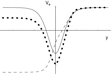
Figure 1: The potential $V_{+}(y)$ for $\Theta=0$ (solid line) and for two non-vanishing values of $\Theta$. The dashed line represents a potential such that there is only one turning point for zero energy.

The Schrödinger equation in this commutative case has a discrete spectrum of bound states and when $\bar{M}$ is of the form (3.55) one of these bound states has zero energy. When $\Theta\not=0$ the shape of $V_{\pm}$ is deformed (see figure 1) and it might happen that there is no discrete bound state spectrum such that includes the zero-energy level. In order to avoid this last possibility it is clear that one should have two turning points at zero energy and, thus, the potential must be such that $\lim_{y\rightarrow\pm\infty}\,V_{\pm}(y)\geq 0$. From the explicit expression of $V_{\pm}(y)$ given in eq. (3.58) one readily proves that:

$$\lim_{y\rightarrow+\infty}\,V_{\pm}(y)\,=\,(l+1)^{2}\,\,,$$

$$\lim_{y\rightarrow-\infty}\,V_{\pm}(y)\,=\,(l+1)^{2}\mp{4\bar{\Theta}^{2}\bar{k}_{01}\over(1+\bar{\Theta}^{4})^{2}}\,\,.$$ (3.59)

It is clear from (3.59) that the potential $V_{-}$ for the $-$modes is always positive at $y=\pm\infty$. However, by inspecting the right-hand side of eq. (3.59) one easily realizes this is not the case for the $+$modes. Actually, from the condition $\lim_{y\rightarrow-\infty}\,V_{+}(y)\geq 0$ we get the following upper bound on $k_{01}$:

$$\bar{k}_{01}\,\leq\,k_{*}(\bar{\Theta})\,\,,\quad\quad{\rm(+modes)}\,\,,$$ (3.60)

where the function $k_{*}(\bar{\Theta})$ is defined as:

$$k_{*}(\bar{\Theta})\,\equiv\,{(1+\bar{\Theta}^{4})^{2}\over 4\bar{\Theta}^{2}}\,\,(l+1)^{2}\,\,.$$ (3.61)

In terms of the original unrescaled quantities, the above bound becomes:

$$k_{01}\,\leq\,{L\over R^{2}}\,{(1+\Theta^{4}\,L^{4})^{2}\over 4\Theta^{2}L^{2}}\,\,(l+1)^{2}\,\,.$$ (3.62)

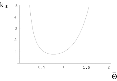
Figure 2: The function $k_{*}(\bar{\Theta})$ for $l=0$.

For a given value of the momentum $k_{1}$ along the $x^{1}$ direction, the above inequality gives a bound on the energy $k_{0}$ of the $+$modes which resembles the stringy exclusion principle. Indeed, as in string theory, we are dealing with a theory with a fundamental length scale. In such theories one expects that it would be imposible to explore distances smaller than the fundamental length which, in turn, implies that some sort of upper bound on the energy and momentum must hold. The function $k_{*}(\Theta)$ has been plotted in figure 2. Notice that this upper bound is infinity when $\Theta\rightarrow 0$ (as it should) but also grows infinitely when $\Theta\rightarrow\infty$. Actually the function $k_{*}(\bar{\Theta})$ satisfies the following duality relation:

$$k_{*}(\bar{\Theta})\,=\,\bar{\Theta}^{4}\,k_{*}({1\over\bar{\Theta}})\,\,.$$ (3.63)

A simple analysis of the function $k_{*}(\bar{\Theta})$ reveals that it has a minimum at a value of $\bar{\Theta}$ equal to

$$\bar{\Theta}_{0}\,=\,{1\over\root 4 \of{3}}\,\approx\,0.7598\,\,,$$ (3.64)

where it reaches the value $k_{*}(\bar{\Theta}_{0})\,=\,{4\over 3\sqrt{3}}\,(l+1)^{2}\approx 0.7698\,(l+1)^{2}$.

Notice that the upper bound (3.60) satisfied by the $+$modes implies, in particular, that the spectrum of these modes is not an infinite tower as in the $\Theta=0$ case (see eq. (3.55)). Instead, we will have a discrete set of values of $\bar{M}$ which, for a given value of $l$, is parametrized by an integer $n$ such that $n\leq n_{*}(\Theta)$, where $n_{*}(\Theta)$ is a function of the non-commutative parameter which diverges when $\Theta=0,\infty$. Actually, we will find below that, for some intermediate values of $\Theta$, there are no $+$modes satisfying the bound (3.60), i.e. they disappear from the spectrum.

Another interesting conclusion that one can extract from the analysis of the potential $V_{\pm}(y)$ in eq. (3.58) is the fact that for $\bar{\Theta}$ sufficiently large the potential, and therefore the spectrum, reduces to the one corresponding to the commutative theory. Indeed, as shown in the plots of figure 1, $V_{\pm}(y)$ is the same for all values of $\bar{\Theta}$ in the region $y\rightarrow+\infty$. On the contrary, the limit of $V_{\pm}(y)$ when $y\rightarrow-\infty$ does depend on $\bar{\Theta}$ (see eq. (3.59)). However, it follows from eq. (3.59) that when $\bar{\Theta}^{6}>>\bar{k}_{01}$ the $\bar{\Theta}$-dependent term of $\lim_{y\rightarrow-\infty}\,V_{\pm}(y)$ can be neglected and, actually, when this condition for $\bar{\Theta}$ is satisfied the form of $V_{\pm}(y)$ in the whole range of $y$ is approximately the same as in the $\bar{\Theta}=0$ case. We will verify below, both analytically and numerically, that the spectrum for $\bar{\Theta}\rightarrow\infty$ reduces to the one in the commutative theory. This fact, which might seem surprising at first sight, is reminiscent of the Morita duality between irreducible modules over the non-commutative torus (see [20] and references therein).

4 Meson spectrum

In this section we will analyze in detail the solution of the differential equations (3.51) for the $\pm$modes. The goal of this analysis is to determine the meson spectrum of the corresponding non-commutative field theory at strong coupling. We will first study this spectrum in the framework of the semiclassical WKB approximation, which has been very successful [36] in the calculation of the glueball spectrum in the context of the gauge/gravity correspondence [37]. The WKB approximation is only reliable for small $\Theta$ and large principal quantum number $n$, although in some cases it turns out to give the exact result. In our case it would provide us of analytical expressions for the energy levels, which will allow us to extract the main characteristics of the spectrum. We will confirm and enlarge the WKB results by means of a numerical analysis of the differential equations (3.51).

4.1 WKB quantization

The standard WKB quantization rule for the Schrödinger equation (3.56) is:

$$(n+{1\over 2})\pi\,=\,\int_{y_{1}}^{y_{2}}\,dy\,\sqrt{-V_{\pm}(y)}\,\,,\,\,\,\,\,\,\,\,\,\,\,\,\,\,n\geq 0\,\,,$$ (4.1)

where $n\in{\rm Z}\kern-3.8pt{\rm Z}\kern 2.0pt$ and $y_{1}$ and $y_{2}$ are the turning points of the potential (3.58) ($V_{\pm}(y_{1})=V_{\pm}(y_{2})=0$). One can evaluate the right-hand side of eq. (4.1) by expanding it as a power series in $1/\bar{M}$. By keeping the leading and subleading terms of this expansion, one can obtain $\bar{M}$ as a function of the quantum number $n$. The explicit calculation for the potential (3.58) (which makes use of the results of [36, 35]) has been performed in appendix A. The expression of $\bar{M}$ one arrives at is:

$$\bar{M}^{2}_{WKB}\,=\,4(n+1)\,\Bigg{(}n+l+1+(l+1)\sqrt{1\mp{\bar{k}_{01}\over k_{*}(\bar{\Theta})}}\,\,\Bigg{)}\,\,.$$ (4.2)

Notice that this spectrum only makes sense if the condition (3.60) is satisfied. When $\bar{\Theta}=0$ the above formula is exact for $l=0$ and for non-vanishing $l$ it reproduces exactly the quadratic and linear terms in $n$. In general, as we will check by comparing it with the numerical results, eq. (4.2) is a good approximation for small $\bar{\Theta}$ and $n>>2(l+1)$. Notice also that, due to the property (3.63) of $k_{*}(\bar{\Theta})$, the spectrum for $\bar{\Theta}\rightarrow\infty$ is identical to that for $\bar{\Theta}\rightarrow 0$.

Let us now analyze some of the consequences of eq. (4.2). Notice first of all that, as $\bar{k}_{01}$ and $\bar{M}$ are related as in eq. (3.53), eq. (4.2) is really an equation which must be solved to obtain $\bar{M}_{WKB}$ as a function of $\bar{k}_{23}$ for given quantum numbers $n$ and $l$. Let us illustrate this fact when $n=l=\bar{k}_{23}=0$. In this case $\bar{k}_{01}=\bar{M}$ and by a simple manipulation of eq. (4.2) one can verify that $\bar{M}_{WKB}$ is obtained by solving the equation:

$$F_{\pm}(\bar{M}_{WKB})\,\equiv\,{\bar{M}_{WKB}^{3}\over 16}\,-\,{\bar{M}_{WKB}\over 2}\,\pm\,{1\over k_{*}(\bar{\Theta})}\,=\,0,$$ (4.3)

where the two signs correspond to those in eq. (4.2). The function $F_{\pm}(\bar{M}_{WKB})$ has a unique minimum at a value of $\bar{M}_{WKB}=\bar{M}_{*}=\sqrt{{8\over 3}}$, where it takes the value:

$$F_{\pm}(\bar{M}_{*})\,=\,-{\sqrt{8}\over 3\sqrt{3}}\pm{1\over k_{*}(\bar{\Theta})}\,\,.$$ (4.4)

Obviously, the equation $F_{\pm}(\bar{M}_{WKB})=0$ has a solution for positive $\bar{M}_{WKB}$ iff $F_{\pm}(\bar{M}_{*})\leq 0$. This condition is satisfied for all values of $\bar{\Theta}$ for $F_{-}$, whereas for $F_{+}$ the non-commutative parameter must be such that

$$k_{*}(\bar{\Theta})\,\geq{3\sqrt{3}\over\sqrt{8}}\,\,,\quad\quad{\rm(+modes)}\,\,.$$ (4.5)

From the form of the function $k_{*}(\bar{\Theta})$ we conclude that the above inequality is satisfied when $\bar{\Theta}\leq\bar{\Theta}_{1}$ and $\bar{\Theta}\geq\bar{\Theta}_{2}$, where $\bar{\Theta}_{1}$ and $\bar{\Theta}_{2}$ are the two solutions of the equation $k_{*}(\bar{\Theta})=3\sqrt{3}/\sqrt{8}$. By numerical calculation one obtains the following values of $\bar{\Theta}_{1}$ and $\bar{\Theta}_{2}$:

$$\bar{\Theta}_{1}\,\approx\,0.376\,\,,\,\,\,\,\,\,\,\,\,\,\bar{\Theta}_{2}\,\approx\,1.239\,\,,\,\,\,\,\,\,\,\,\,\,\,\,({\rm WKB})\,.$$ (4.6)

Therefore, the ground state for the $+$modes disappears from the spectrum if $\bar{\Theta}_{1}<\bar{\Theta}<\bar{\Theta}_{2}$. One can check similarly that the modes with $n>0$ also disappear if $\bar{\Theta}_{1}<\bar{\Theta}<\bar{\Theta}_{2}$ . Thus $(\bar{\Theta}_{1},\bar{\Theta}_{2})$ is a forbidden interval of the non-commutative parameter for the $+$modes. Moreover, notice that the condition (3.60) reduces in this $k_{23}=0$ case to the inequality $\bar{M}\leq k_{*}(\bar{\Theta})$. One can check that when $\bar{\Theta}\,=\bar{\Theta}_{1,2}$ the bound (3.60) is indeed satisfied, since $\bar{M}=\sqrt{{8\over 3}}<k_{*}(\bar{\Theta}_{1,2})=3\sqrt{3}/\sqrt{8}$.

For a non-vanishing value of $\bar{\Theta}$ the energy levels of the $+$modes are cut off at some maximal value $n_{*}(\bar{\Theta})$ of the quantum number $n$. If we consider states with zero momentum $\bar{k}_{23}$ in the non-commutative plane, for which $\bar{M}=\bar{k}_{01}$, the function $n_{*}(\bar{\Theta})$ can be obtained by solving the equation

$$\bar{M}^{2}_{WKB}\Big{|}_{n=n_{*}(\bar{\Theta})}\,=\,k_{*}(\bar{\Theta})^{2}\,\,,$$ (4.7)

where the left-hand side is given by the solution of eq. (4.2). One can get an estimate of $n_{*}(\bar{\Theta})$ for small and large values of $\bar{\Theta}$ by putting $k_{*}(\bar{\Theta})\rightarrow\infty$ on the left-hand side of eq. (4.7). In this case eq. (4.2) yields immediately the value of $\bar{M}$ and if, moreover, we consider states with $l=0$, one arrives at the approximate equation:

$$4(\,n_{*}\,+\,1\,)\,(\,n_{*}\,+\,2\,)\,\approx\,k_{*}(\bar{\Theta})^{2}\,\,,$$ (4.8)

which can be easily solved, namely:

$$n_{*}(\bar{\Theta})\approx-{3\over 2}\,+\,{1\over 2}\,\sqrt{1\,+\,k_{*}(\bar{\Theta})^{2}}\,\,.$$ (4.9)

4.2 Numerical results

We would like now to explore numerically the spectrum of values of $\bar{M}$ for the differential equation (3.51). With this purpose in mind, let us first study the behavior of the solutions of the equation (3.51) for small values of the radial variable $\varrho$. In particular we will try to find a solution of the form:

$$\xi_{\pm}\sim\varrho^{\lambda}\,\,.$$ (4.10)

For small $\varrho$, the term containing $\bar{M}^{2}$ in eq. (3.51) can be neglected and we find that $\varrho^{\lambda}$ is a solution of (3.51) if $\lambda$ satisfies the quadratic equation

$$\lambda^{2}\,+\,2\lambda\,-\,l(l+2)\,\pm\,{4\bar{\Theta}^{2}\bar{k}_{01}\over(1+\bar{\Theta}^{4})^{2}}\,=\,0\,\,,$$ (4.11)

where the two signs correspond to those of eq. (3.51). There are two solutions of the quadratic equation (4.11). The solution that corresponds in the $\bar{\Theta}=0$ limit to the function (3.55) is:

$$\lambda\,=\,-1+(l+1)\,\sqrt{1\mp{\bar{k}_{01}\over k_{*}(\bar{\Theta})}}\,\,,$$ (4.12)

where $k_{*}(\bar{\Theta})$ is the function defined in eq. (3.61). Plugging the value of these exponents $\lambda$ on eq. (4.10), we obtain the behaviour of the $\xi_{\pm}$ fluctuations in the IR, namely:

$$\xi_{\pm}\sim\varrho^{-1+(l+1)\,\sqrt{1\mp{\bar{k}_{01}\over k_{*}(\bar{\Theta})}}}\,\,,\qquad\qquad\qquad(\varrho\sim 0)\,\,.$$ (4.13)

As $k_{*}(\bar{\Theta})\rightarrow\infty$ when $\bar{\Theta}\rightarrow 0$, it is straightforward to verify that eq. (4.13) reduces to $\xi_{\pm}\sim\varrho^{l}$ when $\bar{\Theta}=0$ and thus, as claimed above, the IR behaviour of $\xi_{\pm}$ coincides with the one corresponding to the commutative fluctuations when the non-commutative deformation is switched off. Moreover, it is interesting to notice that the condition $\bar{k}_{01}\leq k_{*}(\bar{\Theta})$ for the $+$modes (eq. (3.60)) appears naturally if we require $\xi_{+}$ to be real in the IR.

In order to obtain the spectrum of values of $\bar{M}$, let us study the behaviour of $\xi_{\pm}$ for large values of $\varrho$. When $\varrho\rightarrow\infty$, the terms containing $\bar{M}^{2}$ and $\bar{k}_{01}$ in eq. (3.51) can be neglected and one can find a solution which behaves as $\xi_{\pm}\sim\varrho^{\Lambda}$ for large $\varrho$. An elementary calculation shows that there are two possible solutions for the exponent $\Lambda$, namely $\Lambda=l,-(l+2)$. Therefore, the general behavior of $\xi_{\pm}$ for large $\varrho$ will be of the form:

$$\xi_{\pm}\,\sim\,c_{1}\,\varrho^{l}\,+\,c_{2}\,\varrho^{-(l+2)}\,\,,\qquad\qquad\qquad(\varrho\sim\infty)\,\,,$$ (4.14)

where $c_{1}$ and $c_{2}$ are constants. The allowed solutions are those which vanish at infinity, i.e. those for which the coefficient $c_{1}$ in (4.14) is zero. For a given value of the momentum $\bar{k}_{23}$ in the non-commutative plane, this condition only happens for a discrete set of values of $\bar{M}$, which can be found numerically by solving the differential equation (3.51) for a function which behaves as in eq. (4.13) near $\varrho=0$ and then by applying the shooting technique to determine the values of $\bar{M}$ for which $c_{1}=0$ in eq. (4.14). Proceeding in this way one gets a tower of values of $\bar{M}$, which we will order according to the increasing value of $\bar{M}$. In agreement with the general expectation for this type of boundary value problems, the fluctuation $\xi_{\pm}$ corresponding to the $n^{th}$ mode has $n$ nodes. Moreover, as happened in the WKB approximation, when $\bar{\Theta}\not=0,\infty$ the tower of states for the $+$modes terminates at some maximal value $n=n_{*}$ and, for some values of $\bar{\Theta}$ and $\bar{k}_{23}$, there is no solution for $\xi_{+}$ satisfying the boundary conditions and the bound (3.60) (see below).

Let us now discuss the results of the numerical calculation when the momentum $\bar{k}_{23}$ in the non-commutative direction is zero. In this case one must put $\bar{k}_{01}=\bar{M}$ in the differential equation (3.51) (see eq. (3.53)). For small $\bar{\Theta}$ the numerical results should be close to those given by the WKB equation (4.2). In order to check this fact we compare in the table below the values of $\bar{M}^{2}$ obtained numerically and those given by the WKB formula (4.2) for the $\pm$modes for $l=0$ and $\bar{\Theta}=.1$

$\bar{M}^{2}$ for $+$modes for $l=0$, $\bar{\Theta}=.1$
$n$	Numerical	WKB
0	$7.37$	$7.77$
1	$22.24$	$23.19$
2	$44.67$	$46.24$
3	$74.76$	$76.89$
4	$112.52$	$115.11$
5	$157.94$	$160.85$

$\bar{M}^{2}$ for $-$modes for $l=0$, $\bar{\Theta}=.1$
$n$	Numerical	WKB
0	$8.69$	$8.22$
1	$25.84$	$24.76$
2	$51.35$	$49.58$
3	$85.10$	$82.68$
4	$126.95$	$124.05$
5	$176.90$	$173.66$

We notice that, indeed, the WKB values represent reasonably well the energy levels especially, as it should, when the number $n$ is large.

It is also interesting to analyze the behaviour of the ground state eigenvalue $\bar{M}(n=0,l=0)$ with the non-commutative parameter $\bar{\Theta}$. In figure 3 we plot our numerical results for the $\pm$modes when the momentum $\bar{k}_{23}$ is zero. As expected, when $\bar{\Theta}=0$ we recover the value corresponding to the mass of the lightest meson of the commutative theory. Moreover, if we increase $\bar{\Theta}$ the value of $\bar{M}$ for the $+$modes decreases, until we reach a point from which there is no solution of the boundary value problem satisfying the bound $\bar{M}\leq k_{*}(\bar{\Theta})$ in a given interval $\bar{\Theta}_{1}\leq\bar{\Theta}\leq\bar{\Theta}_{2}$ of the non-commutativity parameter. The numerical values of $\bar{\Theta}_{1,2}$ are slightly different from the WKB result (4.6), namely $\bar{\Theta}_{1}=0.41$, $\bar{\Theta}_{2}=1.37$. It is interesting to notice the jump and the different behaviour of $\bar{M}$ at both sides of the forbidden region. Notice also that, as expected, $\bar{M}$ approaches the commutative result when $\bar{\Theta}$ is very large.

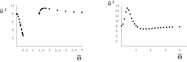
Figure 3: Numerical values of $\bar{M}^{2}$ for the ground state $n=l=0$ for $\bar{k}_{23}=0$ as a function of $\bar{\Theta}$ for $\xi_{+}$ (left) and $\xi_{-}$(right). The corresponding value of the commutative theory is $\bar{M}^{2}=8$.

For the $-$modes there is always a solution for the ground state for all values of $\bar{\Theta}$ and, again, the corresponding value of $\bar{M}$ equals the commutative result when $\Theta=0,\infty$. Interestingly, the range of values of $\bar{\Theta}$ for which $\bar{M}$ differs significantly from its commutative value is approximately the same as the forbidden interval for the $+$modes (see figure 3).

The differential equations for our fluctuations break explicitly the Lorentz invariance among the Minkowski coordinates $x^{0}\cdots x^{3}$. In order to find out how this breaking is reflected in the spectrum it is interesting to study the values of $\bar{M}^{2}$ for $\bar{k}_{23}\not=0$. In this case $\bar{k}_{01}\not=\bar{M}$ (see eq. (3.53)) and one can regard $\bar{k}_{23}$ as a external parameter in our boundary value problem. When $\bar{\Theta}\not=0$ the values of $\bar{M}$ that one obtains by solving the differential equation (3.51) do depend on $\bar{k}_{23}$. This dependence encodes the modification of the relativistic dispersion relation due to the non-commutative deformation. For illustrative purposes let us consider the spectrum for the $+$modes. The values of $\bar{M}^{2}$ as a function of $\bar{k}_{23}$ for the ground state ($n=l=0$) and two different values of $\bar{\Theta}$ are shown in figure 4. Notice that, as a consequence of (3.60), the momentum $\bar{k}_{23}$ is bounded from above. Moreover, $\bar{M}^{2}$ increases (decreases) with $\bar{k}_{23}$ when $\bar{\Theta}<\bar{\Theta}_{1}$ ($\bar{\Theta}>\bar{\Theta}_{2}$), while it becomes independent of $\bar{k}_{23}$ as $\Theta\rightarrow 0,\infty$.

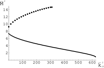
Figure 4: Numerical values of $\bar{M}^{2}$ for the ground state $n=l=0$ of the $+$modes as a function of $\bar{k}_{23}=0$ for two different values of $\bar{\Theta}$. The continuous line corresponds to $\bar{\Theta}=0.1<\bar{\Theta}_{1}$, while the dotted line are the values of $\bar{M}^{2}$ for $\bar{\Theta}=2>\bar{\Theta}_{2}$.

5 Semiclassical strings in the non-commutative background

Let us now study the meson spectrum for large four-dimensional spin. An exact calculation of this spectrum would require the analysis of the fluctuations of open strings attached to the D7-brane in the non-trivial gravitational background of section 2. This calculation is not feasible, even for the case of D7-branes in the $AdS_{5}\times S^{5}$ geometry considered in ref. [7]. However, for large four-dimensional spin we can treat the open strings semiclassically, as suggested in ref. [38]. In this approach one solves the classical equations of motion of rotating open strings with appropriate boundary conditions. These equations are rather complicated and can only be solved numerically. However, from these numerical solutions we will be able to extract the energy and angular momentum of the string and study how they are correlated. The analysis for the commutative $\Theta=0$ case was performed in ref. [7]. Here we would like to explore the effect of a non-commutative deformation on the behavior found in ref. [7].

5.1 Strings rotating in the non-commutative plane

As explained above, the spectrum of mesons with large four-dimensional spin can be obtained from classical rotating open strings. In order to study these configurations let us consider strings attached to the D7 flavor brane, extended in the radial direction, and rotating in the $x^{2}x^{3}$ plane (i.e. in the non-commutative directions). The relevant part of the metric is:

$${r^{2}\over R^{2}}\left[-dt^{2}+h\left(\left(dx^{2}\right)^{2}+\left(dx^{3}\right)^{2}\right)\right]+{R^{2}\over r^{2}}dr^{2}.$$ (5.1)

Defining the coordinate $z$ as

$$z={R^{2}\over r}\,\,,$$ (5.2)

and changing to polar coordinates on the $x^{2}x^{3}$ plane, the metric above becomes:

$${R^{2}\over z^{2}}\left[-dt^{2}+h\left(d\rho^{2}+\rho^{2}d\theta^{2}\right)+dz^{2}\right]\,\,,$$ (5.3)

where $h$ and $B$, in terms of the new coordinate $z$, are

$$h = \left(1+R^{8}{\Theta^{4}\over z^{4}}\right)^{-1},$$

$$B = -\Theta^{2}{r^{4}\over R^{2}}h\,\rho\,d\rho\wedge d\theta=-\Theta^{2}{R^{6}\over z^{4}}h\,\rho\,d\rho\wedge d\theta.$$ (5.4)

Notice that the coordinate $\rho$ introduced above as radial coordinate in the $x^{2}x^{3}$ plane has nothing to do with the one defined in eq. (3.24). Actually, since the string is rotating around one of its middle points, we must allow $\rho$ to have negative values. Let us now consider an open fundamental string moving in the above background. Let $(\tau,\sigma)$ be worldsheet coordinates. The embedding of the string will be determined by the functions $X^{M}(\sigma,\tau)$, where $X^{M}$ represent the target space coordinates. Moreover, the dynamics of the string is governed by the standard Nambu-Goto action

$$S=-{1\over 2\pi\alpha^{\prime}}\int d\tau\,d\sigma\sqrt{-\det g}+{1\over 2\pi\alpha^{\prime}}\int P[B]\,\,,$$ (5.5)

where $g$ is the metric induced on the worldsheet of the string. Let us write the form of the action (5.5) for the following ansatz:

$$t=\tau\>,\>\theta=\omega\tau\>,\>\rho=\rho(\sigma)\>,\>z=z(\sigma),$$ (5.6)

where $\omega$ is a constant angular velocity. If the prime denotes derivative with respect to $\sigma$, the determinant of the induced metric and the pullback of the $B$ field for the ansatz (5.6) are given by:

$$\sqrt{-\det g}={R^{2}\over z^{2}}\sqrt{\left(1-h\,\rho^{2}\omega^{2}\right)\left(h\,\rho^{\prime 2}+z^{\prime 2}\right)},$$ (5.7)

$$P[B]=\Theta^{2}{R^{6}\over z^{4}}h\,\rho\,\omega\,\rho^{\prime}\,d\tau\wedge d\sigma\,\,.$$ (5.8)

By plugging this result on the action (5.5) one finds the following lagrangian density:

$${\cal L}={R^{2}\over 2\pi\alpha^{\prime}}\left(-{1\over z^{2}}\sqrt{\left(1-h\,\rho^{2}\,\omega^{2}\right)\left(h\,\rho^{\prime 2}+z^{\prime 2}\right)}+\Theta^{2}{R^{4}\over z^{4}}h\,\rho\,\omega\,\rho^{\prime}\right).$$ (5.9)

The lagrangian (5.9) does not depend explicitly on $t$ and $\theta$. Therefore, our system has two conserved quantities: the energy $E$ and the (generalized) angular momentum $J$, whose expressions are given by:

$$E = \omega{\partial S\over\partial\omega}-S={R^{2}\over 2\pi\alpha^{\prime}}\int d\sigma{\sqrt{h\,\rho^{\prime 2}+z^{\prime 2}}\over z^{2}\sqrt{1-h\,\rho^{2}\omega^{2}}}\,,$$

$$J = {\partial S\over\partial\omega}={R^{2}\over 2\pi\alpha^{\prime}}\left[\int d\sigma\left({h\,\rho^{2}\omega\over z^{2}}{\sqrt{h\,\rho^{\prime 2}+z^{\prime 2}}\over\sqrt{1-h\,\rho^{2}\omega^{2}}}+\Theta^{2}{R^{4}\over z^{4}}h\,\rho\,\rho^{\prime}\right)\right]\,\,.$$ (5.10)

The physical angular momentum of the string is given by the first term on the second equation in (5.1), namely:

$$J_{1}={R^{2}\over 2\pi\alpha^{\prime}}\int d\sigma{h\rho^{2}\omega\over z^{2}}{\sqrt{h\,\rho^{\prime 2}+z^{\prime 2}}\over\sqrt{1-h\,\rho^{2}\omega^{2}}}\,\,.$$ (5.11)

The equations of motion defining the time-independent profile of the string can be obtained from (5.9). Moreover, in addition one must impose the boundary conditions that make the action stationary:

$${\partial L\over\partial(X^{\prime})^{M}}\delta X^{M}\Big{|}_{\partial\Sigma}=0\,\,.$$ (5.12)

As the endpoints of the string are attached to the flavor brane placed at constant $z$, $\delta z|_{\partial\Sigma}=0$. Moreover, since $\delta\rho\big{|}_{\partial\Sigma}$ is arbitrary, the condition (5.12) reduces to:

$${\partial{\cal L}\over\partial\rho\,^{\prime}}\Bigg{|}_{\partial\Sigma}=0\,\,.$$ (5.13)

Taking into account the explicit form of ${\cal L}$ (eq. (5.9)), one can rewrite eq. (5.13) as:

$${\sqrt{1-h\,\rho^{2}\omega^{2}}\over\sqrt{h\,\rho^{\prime 2}+z^{\prime 2}}}\,\,\rho^{\prime}\,\Bigg{|}_{\partial\Sigma}={R^{4}\Theta^{2}\over z^{2}}\,\rho\omega\,\Bigg{|}_{\partial\Sigma}\,\,.$$ (5.14)

Eq. (5.14) can be used to find the angle at which the string hits the flavor brane. Indeed, let us suppose that the D7-brane is placed at $z=z_{D7}$ and that the string intercepts the D7-brane at two points with coordinates $\rho=-\tilde{\rho}_{D7}<0$ and $\rho=\rho_{D7}>0$. We will orient the string by considering the $\rho=-\tilde{\rho}_{D7}$ ($\rho=\rho_{D7}$) end as its initial (final) point. It follows straightforwardly from eq. (5.14) that the signs of $d\rho/d\sigma$ at the two ends of the string are:

$${d\rho\over d\sigma}\,\Bigg{|}_{\rho=-\tilde{\rho}_{D7}}\,\leq\,0\,\,,\qquad\qquad\qquad{d\rho\over d\sigma}\,\Bigg{|}_{\rho=\rho_{D7}}\,\geq\,0\,\,.$$ (5.15)

Notice that for $\Theta=0$ the right-hand side of eq. (5.14) vanishes, which means that $\rho^{\prime}_{|\partial\Sigma}=0$ and, therefore, the string ends orthogonally on the D7-brane, in agreement with the results of ref. [7]. Moreover, $\tilde{\rho}_{D7}\,=\,\rho_{D7}$ in the commutative case and the string configuration is symmetric around the point $\rho=0$ (see ref. [7]). On the contrary, eq. (5.14) shows that $\rho^{\prime}_{|\partial\Sigma}$ does not vanish in the non-commutative theory and, thus, the string hits the D7-brane at a certain angle, which depends on the non-commutative parameter $\Theta$ and on the $\rho$ and $z$ coordinates of $\partial\Sigma$. Actually, it follows from the signs displayed in eq. (5.15) that the string profile is not symmetric around $\rho=0$ when $\Theta\not=0$ and that the string is tilted towards the region of negative $\rho$. The actual values of $dz/d\rho$ at the two ends of the string can be obtained by solving the quadratic equation for $z^{\prime}/\rho^{\prime}$ in (5.14). One gets:

$${dz\over d\rho}\Bigg{|}_{\rho=-\tilde{\rho}_{D7}}=-{\,z_{D7}^{2}\sqrt{1-\tilde{\rho}_{D7}^{2}\,\omega^{2}}\over\hat{\Theta}^{2}\,\tilde{\rho}_{D7}\,\omega}\,\,,\qquad\quad\qquad{dz\over d\rho}\Bigg{|}_{\rho=\rho_{D7}}=-{\,z_{D7}^{2}\sqrt{1-\rho_{D7}^{2}\,\omega^{2}}\over\hat{\Theta}^{2}\,\rho_{D7}\,\omega}\,\,,$$ (5.16)

where the sign of the right-hand side has been chosen to be in agreement with eq. (5.15) and we have defined $\hat{\Theta}=\Theta\,R^{2}$.

Setting $\sigma=\rho$, the equation of motion defining the string profile $z(\rho)$ can be easily obtained from the lagrangian (5.9):

$$h{z^{\prime\prime}\over h+z^{\prime 2}}-{h\,\rho\,\omega^{2}\over 1-h\,\rho^{2}\omega^{2}}z^{\prime}-{4\hat{\Theta}^{2}\over z^{3}}h^{2}\rho\,\omega\sqrt{{h+z^{\prime 2}\over 1-h\,\rho^{2}\omega^{2}}}+$$

$$+{2h^{2}\over z\left(1-h\,\rho^{2}\omega^{2}\right)\left(h+z^{\prime 2}\right)}\Bigg{\{}z^{\prime 2}\left[1-{\hat{\Theta}^{4}\over z^{4}}+\rho^{2}\omega^{2}\left(1-2h+{\hat{\Theta}^{4}\over z^{4}}h\right)\right]+$$

$$+h\left[1-\rho^{2}\omega^{2}h\left(1-{\hat{\Theta}^{4}\over z^{4}}\right)\right]\Bigg{\}}=0,$$ (5.17)

where now $z^{\prime}={dz\over d\rho}$. In order to solve the second-order differential equation (5.17) we need to impose the value of $z$ and $z^{\prime}$ at some value of $\rho$. Clearly, the boundary condition (5.16) fixes $z^{\prime}$ at $\rho=\rho_{D7}$. Since the string intersects the D7-brane at this value of $\rho$, it is evident that we have to impose also that:

$$z(\rho=\rho_{D7})=z_{D7}\,\,.$$ (5.18)

By using the initial conditions (5.16) at $\rho=\rho_{D7}$ and (5.18), the equation of motion (5.17) can be numerically integrated for given values of $z_{D7}$, $\rho_{D7}$ and $\omega$. It turns out that these values are not uncorrelated. Indeed, we still have to satisfy the condition written in eq. (5.16) for $z^{\prime}(\rho=-\tilde{\rho}_{D7})$, which determines the angle at which the $\rho=-\tilde{\rho}_{D7}$ end of the string hits the brane and it is not satisfied by arbitrary values of $z_{D7}$, $\rho_{D7}$ and $\omega$. Actually, let us consider a fixed value of $z_{D7}$. Then, by requiring the fulfillment of eq. (5.16), one gets a relation between the quark-antiquark separation $\rho_{D7}+\tilde{\rho}_{D7}$ and the angular velocity $\omega$. Before discussing this relation let us point out that, due to the tilting of the string, the coordinate $\rho$ is not a good global worldvolume coordinate in the region of negative $\rho$, since $z(\rho)$ is a double-valued function in that region. In order to overcome this problem we will solve eq. (5.17) for $z(\rho)$ starting at $\rho=\rho_{D7}$ until a certain negative value of $\rho$ and beyond that point we will continue the curve by parametrizing the string by means of a function $\rho=\rho(z)$. The differential equation governing the function $\rho(z)$, which is similar to the one written in (5.17) for $z(\rho)$, can be easily obtained from the lagrangian density (5.9) after taking $\sigma=z$. We have solved this equation by using as initial conditions the values of the coordinate and slope of the last point of the $z=z(\rho)$ curve. By performing the numerical integration in this way, the $\rho(z)$ curve is continued until $z=z_{D7}$. Then $\tilde{\rho}_{D7}$ is determined as $-\tilde{\rho}_{D7}=\rho(z_{D7})$ and one can check whether or not the string hits the flavor brane at $\rho=-\tilde{\rho}_{D7}$ with the angle of eq. (5.16). For a given value of the angular velocity $\omega$ this only happens for some particular values of $\rho_{D7}$ and $\tilde{\rho}_{D7}$. Some of the profiles found by numerical integration are shown in figure 5. As explained above these curves are tilted in general. This tilting increases with the non-commutative parameter and, for fixed $\Theta\not=0$, it becomes more drastic as $\omega$ grows.

As mentioned above, for a given value of $z_{D7}$ the fulfillment of the conditions written in eq. (5.16) determines a relation between $\tilde{\rho}_{D7}$, $\rho_{D7}$ and $\omega$. In order to characterize this relation let us define $\bar{\rho}_{D7}$ as the half of the quark-antiquark separation, i.e. $2\bar{\rho}_{D7}\,=\,\tilde{\rho}_{D7}+\rho_{D7}$. In figure 6 we have represented $\bar{\rho}_{D7}$ as a function of $\omega$ for some non-vanishing value of $\Theta$. From these numerical results one concludes that $\bar{\rho}_{D7}\rightarrow\infty$ when $\omega\rightarrow 0$, while $\bar{\rho}_{D7}$ vanishes for large $\omega$. Actually, the behaviours found for small and large $\omega$ can be reproduced by a simple power law, namely:

$$\bar{\rho}_{D7}\,\sim\omega^{-{2\over 3}}\,\,,\quad\quad(\omega\rightarrow 0)\,\,,$$

$$\bar{\rho}_{D7}\,\sim\omega^{-{1}}\,\,,\quad\quad(\omega\rightarrow\infty)\,\,.$$ (5.19)

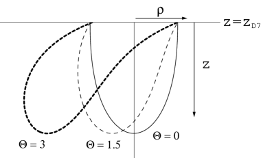
Figure 5: Rotating string profiles for three different values of the non-commutative parameter ($\Theta=$0, 1.5 and 3). The three curves correspond to the same value of $\rho_{D7}$. As $\Theta$ grows the tilting increases. However, the maximal value of $z$ is roughly the same for the three curves.

The power law behaviours displayed in eq. (5.19) coincide with the ones found in ref. [7] for the $AdS_{5}\times S^{5}$ background. They imply, in particular that $\omega\rightarrow 0$ corresponds to having long strings, whereas for $\omega\rightarrow\infty$ we are dealing with very short strings.

Once the profile of the string is known, we can plug it on the right-hand side of eqs. (5.1) and (5.11) and obtain the energy and the angular momentum of the rotating string by numerical integration. As happens for the $AdS_{5}\times S^{5}$ background, large(small) angular velocity corresponds to small (large) values of the angular momentum $J_{1}$. Actually, for small $\omega$ the angular momentum $J_{1}$ diverges, while $J_{1}\rightarrow 0$ for large $\omega$. The spectrum $E(J_{1})$ can be obtained parametrically by integrating the equation of motion for different values of $\omega$. The results for some values of $\Theta$ have been plotted in figure 6. For small $J_{1}$ (or large $\omega$) the meson energy follows a Regge trajectory since the energy $E$ grows linearly with $\sqrt{J_{1}}$. The actual value of the Regge slope can be obtained analytically (see the next subsection). This Regge slope, which is nothing but an effective tension for the rotating string, is independent of $\Theta$ (see figure 6). An explanation of this fact is provided in the next subsection. For intermediate values of $J_{1}$ the $E(J_{1})$ curve does depend on the non-commutative parameter while, on the contrary, for large $J_{1}$ (or small $\omega$) one recovers again the $\Theta=0$ result, since the energy becomes $2m_{q}$, with $m_{q}={R^{2}\over 2\pi\alpha^{\prime}z_{D7}}$ being the mass of the quarks. Actually this last result is quite natural since this large $J_{1}$ region corresponds to large strings and one expects that the effects of the non-commutativity will disappear.

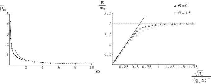
Figure 6: On the left we plot the half of the quark-antiquark separation $\bar{\rho}_{D7}$ as a function of the angular velocity $\omega$. For large $\omega$, $\bar{\rho}_{D7}\approx\omega^{-1}$ (dashed line). In the $\omega\rightarrow 0$ region, $\bar{\rho}_{D7}\sim\omega^{-2/3}$ (solid line). On the right plot we represent the energy versus angular momentum of the rotating string for the commutative and non-commutative theories. The meson masses follow Regge trajectories in the large $\omega$ (small $J_{1}$) region with an effective tension which does not depend on the non-commutative parameter $\Theta$ and is given by eq. (5.29). The linear Regge trajectory given by eq. (5.28) is also plotted for comparison (solid line). For large $J_{1}$ (small $\omega$) which corresponds to long strings, the energy approaches the free value $2m_{q}$. We are setting $z_{D7}=R^{2}=\alpha^{\prime}=1$.

An interpretation of the behaviour of the spectrum in the two limiting regimes (small and large $J_{1}$) was given in ref. [7]. Let us recall, and adapt to our system, the arguments of [7]. For small $J_{1}$ the string is very short and it is not much influenced by the background geometry. As a consequence the spectrum is similar to the one in flat space, i.e. it follows a Regge trajectory with a tension which is just the proper tension $1/2\pi\alpha^{\prime}$ appropriately red-shifted. This effective tension is independent of $\Theta$. However, we will verify in section 6 that this is not the case when computing the static quark-antiquark potential energy. The static and dynamic tensions are different and they only coincide for $\Theta=0$, where we recover the results of ref. [7].

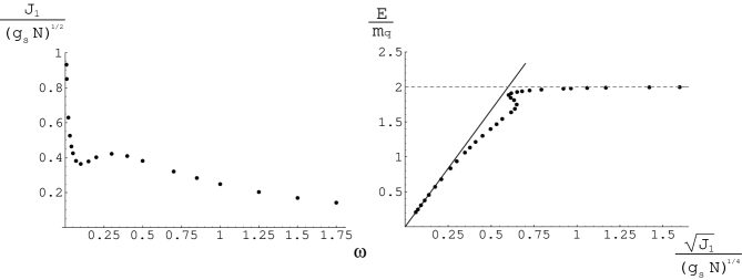
Figure 7: On the left we represent the angular momentum $J_{1}$ versus the angular velocity $\omega$ for $\Theta=3$ and $z_{D7}=1$. The corresponding energy versus angular momentum plot is shown on the right. The solid line corresponds to the linear Regge trajectory (5.28).

For large $J_{1}$ the spectrum corresponds to that of two non-relativistic masses bound by a Coulomb potential. This is in agreement with the fact that in this long distance regime the distance between the quark-antiquark pair is much larger than the inverse mass of the lightest meson and one expects large screening corrections to the potential. We will confirm this result by means of a static calculation, where we will compute the non-commutative corrections to the large distance potential.

For $\Theta=0$ the $E(J_{1})$ curve interpolates smoothly between the Regge behaviour at small $J_{1}$ and the Coulomb regime at large $J_{1}$. However, when $\Theta$ is non-vanishing and large enough, the crossover region is more involved since, in some interval of $J_{1}$, the energy decreases with increasing angular momentum. By analyzing the numerical results of $J_{1}$ as a function of $\omega$ (see figure 7), one can easily conclude that this effect is due to the fact that, when $\Theta$ is large, the angular momentum $J_{1}$ has some local extremum for some intermediate values of $\omega$.

5.1.1 Large angular velocity

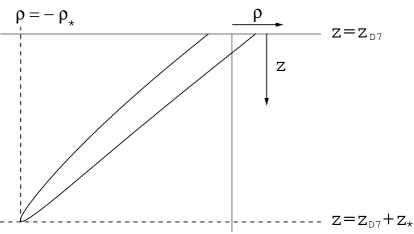
Figure 8: The string profile for large angular velocity.

Let us now analyze the case $\omega\rightarrow\infty$. As we have checked by numerical computation, the solution in this limit consists of a very short string with $\rho_{D7}=1/\omega$ and $z(\rho)\approx z_{D7}$. Actually, for large $\omega$ the shape of the string resembles two nearly parallel straight lines joined at some turning point (see figure 8). Let $\rho=-\rho_{*}$ be the $\rho$ coordinate of the turning point. The value of $\rho_{*}$ can be approximately obtained by noticing that $d^{2}z/d\rho^{2}$ should diverge at $\rho=-\rho_{*}$. By inspecting the differential equation (5.17) one readily realizes that this can only happen if $1-h\rho^{2}\omega^{2}$ vanishes. Taking into account that the coordinate $z$ is very close to $z_{D7}$ for these short strings, one concludes that:

$$\rho_{*}\,\approx\,{1\over h_{D7}^{{1\over 2}}\,\,\omega}\,\,,$$ (5.20)

where

$$h_{D7}=\left(1+{\hat{\Theta}^{4}\over z_{D7}^{4}}\right)^{-1}\,\,.$$ (5.21)

Let $z_{D7}+z_{*}$ be the value of the function $z(\rho)$ at $\rho=-\rho_{*}$ (see figure 8). It is clear that $z_{*}$ measures how far the rotating string is extended in the holographic direction. Our numerical calculations show that, for a given value of the angular velocity $\omega$, the tilting of the string grows as $\Theta$ is increased but $z_{*}$ remains nearly the same. Let us check this fact from the above equations for large values of $\hat{\Theta}$. Indeed, in this case we can obtain approximately $z_{*}$ by multiplying the slope (5.16) by $\rho_{*}$, namely:

$$z_{*}\,\approx\,-{dz\over d\rho}\Bigg{|}_{\rho=\rho_{D7}}\rho_{*}\,\,.$$ (5.22)

Moreover, the expression (5.20) of $\rho_{*}$ for large $\hat{\Theta}$ reduces to:

$$\rho_{*}\,\approx\,{\hat{\Theta}^{2}\over z_{D7}^{2}\omega}\,\,,$$ (5.23)

and using (5.16) to evaluate the right-hand side of eq. (5.22), one gets:

$$z_{*}\,\approx\,{\sqrt{1-\rho_{D7}^{2}\omega^{2}}\over\rho_{D7}\omega^{2}}\,\,.$$ (5.24)

Notice that all the $\hat{\Theta}$ dependence has dropped out from the right-hand side of eq. (5.24) and, thus, $z_{*}$ is independent of $\hat{\Theta}$ as claimed. Moreover, by comparing with our numerical calculations we have found that eq. (5.24) represents reasonably well $z_{*}$.

Our numerical results indicate that the energy $E$ and the angular momentum $J_{1}$ do not depend on $\Theta$. Again we can check this fact by computing $E$ and $J_{1}$ for large $\Theta$. Notice that, as $\rho_{D7}\approx 1/\omega$, one gets from (5.23) that $\rho_{D7}/\rho_{*}\approx z_{D7}^{2}/\hat{\Theta}^{2}$ and, therefore, $\rho_{D7}<<\rho_{*}$ if $\hat{\Theta}$ is large and, as a consequence, the profile of the string degenerates into two coinciding straight lines. Therefore, the energy and the angular momentum in this regime can be obtained by taking $z=z_{D7}={\rm constant}$ in eqs. (5.1) and (5.11) and performing the integration of $\rho$ between $\rho=0$ and $\rho=\rho_{*}$:

$$E\,\approx\,2\,{R^{2}\over 2\pi\alpha^{\prime}}\,\,{h_{D7}^{{1\over 2}}\over z_{D7}^{2}}\,\,\int_{0}^{\rho_{*}}\,\,{d\rho\over\sqrt{1-h_{D7}\,\rho^{2}\omega^{2}}}\,\,.$$ (5.25)

By an elementary change of variables, this integral can be done analytically and, after taking into account the expression of $\rho_{*}$ (eq. (5.20)), we get the following expression of $E$:

$$E\approx{R^{2}\over 2\alpha^{\prime}\omega\,z_{D7}^{2}}\,\,.$$ (5.26)

Notice that the dependence of $E$ on $h_{D7}$, and thus on $\Theta$, has disappeared. Similarly, the angular momentum $J_{1}$ can be written as:

$$J_{1}\,\approx\,2\,{R^{2}\over 2\pi\alpha^{\prime}}\,\,{h_{D7}^{{3\over 2}}\,\omega\over z_{D7}^{2}}\,\,\int_{0}^{\rho_{*}}\,\,d\rho{\rho^{2}\over\sqrt{1-h_{D7}\,\rho^{2}\omega^{2}}}\,=\,{R^{2}\over 4\alpha^{\prime}\omega^{2}\,z_{D7}^{2}}\,\,,$$ (5.27)

and $J_{1}$ is also independent of the non-commutative parameter. Notice that $E$ and $J_{1}$ depend on the angular velocity $\omega$ as $E\sim 1/\omega$ and $J_{1}\sim 1/\omega^{2}$. This means that, indeed, $E\sim\sqrt{J_{1}}$ in this large $\omega$ regime and, actually, if we define the effective tension for the rotating string as:

$$\tau_{eff}^{R}\,\equiv\,{E^{2}\over 2\pi J_{1}}\,\,,$$ (5.28)

we have:

$$\tau_{eff}^{R} = {1\over 2\pi\alpha^{\prime}_{eff}}\simeq{R^{2}\over 2\pi\alpha^{\prime}z_{D7}^{2}}\,\,.$$ (5.29)

As argued in ref. [7] for $\Theta=0$, the tension (5.29) can be understood as the proper tension ${1\over 2\pi\alpha^{\prime}}$ at $z=z_{D7}$ which is then red-shifted as seen by a boundary observer.

5.1.2 Small angular velocity

From the numerical computation displayed in figure 6 one can see that, in the large $J_{1}$ region (which corresponds to small $\omega$), the energy becomes: $E\simeq 2m_{q}$, where $m_{q}={R^{2}\over 2\pi\alpha^{\prime}z_{D7}}$ is the mass of the dynamical quarks. Furthermore, as we can see in figure 6, the separation between the string endpoints $\bar{\rho}_{D7}$ when $\omega\rightarrow 0$ behaves as $\omega^{-2/3}$ (see eq. (5.19)), which is the classical result for two non-relativistic particles bound by a Coulomb potential, namely Kepler’s law i.e. the cube of the radius is proportional to the square of the period. This is precisely what one gets in the commutative case. In the next section we will calculate the static quark-antiquark potential for long strings and we will verify that the dominant term of this potential is of the Coulomb form, with a strength which is independent of $\Theta$. Therefore, as expected on general grounds, in this limit the rotating string behaves exactly as in the commutative theory, and this can be understood taking into account that this $\omega\rightarrow 0$ limit corresponds to long strings, much larger than the non-commutativity scale of the theory.

6 Hanging strings

In this section we will evaluate the potential energy for a static quark-antiquark pair and we will compare the result with the calculation of the energy for a rotating string presented in section 5. Following the analysis of ref. [3], let us consider a static configuration consisting of a string stretched in the $x^{3}$ direction with both ends attached to the $D7$-brane probe placed at $r=r_{D7}$. The relevant part of the metric is:

$${r^{2}\over R^{2}}\left[-dt^{2}+h\left(dx^{3}\right)^{2}\right]+{R^{2}\over r^{2}}dr^{2}.$$ (6.1)

Using $x^{3}$ as worldvolume coordinate and considering an ansatz of the form $r=r(x^{3})$, the Nambu-Goto action reads:

$${\cal L}=-{1\over 2\pi\alpha^{\prime}}\sqrt{-\det g}=-{1\over 2\pi\alpha^{\prime}R^{2}}\sqrt{r^{4}h+R^{4}r^{\prime 2}},$$ (6.2)

where $r^{\prime}$ denotes ${dr\over dx^{3}}$. As ${\cal L}$ does not depend explicitly on $x^{3}$, the quantity $r^{\prime}{\partial{\cal L}\over\partial r^{\prime}}-{\cal L}$ is a constant of motion,i.e.:

$${r^{4}h\over\sqrt{R^{4}r^{\prime 2}+r^{4}h}}\,=\,{\rm constant}\,\,.$$ (6.3)

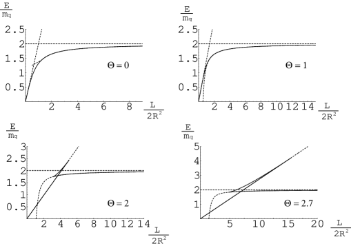
Figure 9: Energy of the static quark-antiquark configuration versus the string length $L$ for $\Theta=0$ (commutative case), $\Theta=1$, $\Theta=2$, and $\Theta=2.7$ (setting $z_{D7}=R^{2}=\alpha^{\prime}=1$). The solid line shows the result of the numeric computation, the straight dashed line displays the Regge behaviour obtained in section 6.1, and the curved dashed line shows the Coulomb potential computed in section 6.2.

The configurations we are interested in are those in which the string is hanging of the flavor brane at $r=r_{D7}$ and reaching a minimum value $r_{0}$ of the coordinate $r$. Since $r^{\prime}=0$ when $r=r_{0}$, we can immediately evaluate the constant of motion and rewrite eq. (6.3) as:

$${r^{4}h\over\sqrt{R^{4}r^{\prime 2}+r^{4}h}}={r_{0}^{2}\over\sqrt{1+\Theta^{4}r_{0}^{4}}}\,\,.$$ (6.4)

From this expression we get readily $r^{\prime}$ in terms of $r$, from which we can compute the string length (i.e. the quark-antiquark separation) with the result:

$$L = 2\int_{r_{0}}^{r_{D7}}{dx^{3}\over dr}dr=2R^{2}\int_{r_{0}}^{r_{D7}}{r_{0}^{2}(1+\Theta^{4}r^{4})\over r^{2}\sqrt{r^{4}-r_{0}^{4}}}dr=$$ (6.5)

$$= {2R^{2}\over r_{0}}\int_{1}^{\frac{r_{D7}}{r_{0}}}{dy\over y^{2}\sqrt{y^{4}-1}}+2R^{2}r_{0}^{3}\,\Theta^{4}\,\int_{1}^{\frac{r_{D7}}{r_{0}}}{y^{2}\over\sqrt{y^{4}-1}}dy\,\,.$$

The energy for this static configuration becomes:

$$E\,=\,-\int{\cal L}\,d\sigma\,=\,{1\over\pi\alpha^{\prime}}r_{0}\sqrt{1+\Theta^{4}\,r_{0}^{4}}\int_{1}^{\frac{r_{D7}}{r_{0}}}{y^{2}\over\sqrt{y^{4}-1}}\,dy\,\,.$$ (6.6)

These last two expressions for $E$ and $L$ can be evaluated numerically for any $r_{0}$ between $0$ and $r_{D7}$. From this result we obtain the energy of the static quark-antiquark configuration as a function of the distance between the quark and the antiquark. These results have been plotted in figure 9, where one can observe that the potential is linear for small quark-antiquark separation, while for large separation the energy becomes constant and equal to $2m_{q}$. Notice that this behaviour is the same as the one we found for the energy of the rotating strings. In the next two subsections we will analyze carefully the small and long separation limits and we will obtain analytical expressions describing the behaviour of the configuration in those limits.

6.1 Short strings limit

The small separation limit $L\rightarrow 0$ is achieved when $r_{0}\rightarrow r_{D7}$. Then, by defining ${r_{D7}\over r_{0}}=1+\epsilon$ and making the change of variable $y=1+z$, it is easy to get, at leading order:

$$L={2R^{2}\over r_{D7}}\left(1+\Theta^{4}r_{D7}^{4}\right)\epsilon^{\frac{1}{2}}\,\,,\qquad\qquad E={r_{D7}\over\pi\alpha^{\prime}}\sqrt{1+\Theta^{4}r_{D7}^{4}}\,\epsilon^{\frac{1}{2}}\,\,.$$ (6.7)

From the dependence of $L$ and $E$ on $\epsilon$ we notice that, indeed, $E=\tau_{eff}^{W}L$, where $\tau_{eff}^{W}$ is the effective tension and is given by:

$$\tau_{eff}^{W}={E\over L}={r_{D7}^{2}\over 2\pi\alpha^{\prime}R^{2}}\,{1\over\sqrt{1+\Theta^{4}r_{D7}^{4}}}={R^{2}\over 2\pi\alpha^{\prime}z_{D7}^{2}}\,{1\over\sqrt{1+\Theta^{4}r_{D7}^{4}}}\,.$$ (6.8)

Notice that $\tau_{eff}^{W}$ decreases with the non-commutative parameter $\Theta$. Actually, the maximal value of $\tau_{eff}^{W}$ is reached when $\Theta=0$, where it has the same value as the tension $\tau_{eff}^{R}$ of the rapidly rotating string (see eq. (5.29)). Therefore, for a general value of $\Theta$ these two tensions have different values.

6.2 Long strings limit

The limit $L\rightarrow\infty$ is achieved by taking the constant of integration $r_{0}\rightarrow 0$. It is easy to see from (6.5), (6.6) that the dependence on $\Theta$ cancels out at leading order. Therefore, the Coulomb behaviour of the commutative theory found in ref. [7] is exactly recovered at long distances. This is expected on general grounds since, at distances bigger than the scale set by the noncommutativity parameter of the field theory, the commutative theory must be obtained. However, let us see what we get beyond the leading term. Since $\frac{r_{D7}}{r_{0}}=\frac{2\pi\alpha^{\prime}m_{q}}{r_{0}}$, the length $L$ in (6.5) can be rewritten as:

$$L={2R^{2}\over r_{0}}\left(\int_{1}^{\infty}{dy\over y^{2}\sqrt{y^{4}-1}}-\int_{\frac{2\pi\alpha^{\prime}m_{q}}{r_{0}}}^{\infty}\,{dy\over y^{2}\sqrt{y^{4}-1}}\right)+2R^{2}r_{0}^{3}\,\Theta^{4}\,\int_{1}^{\frac{2\pi\alpha^{\prime}m_{q}}{r_{0}}}dy{y^{2}\over\sqrt{y^{4}-1}}\,.$$ (6.9)

The first integral in eq. (6.9) can be explicitly computed, namely:

$${\cal C}\equiv\int_{1}^{\infty}{dy\over y^{2}\sqrt{y^{4}-1}}={\sqrt{\pi}\,\Gamma\left({3\over 4}\right)\over\Gamma\left({1\over 4}\right)}\approx 0.59907\,\,.$$ (6.10)

Moreover, when $\frac{r_{D7}}{r_{0}}=\frac{2\pi\alpha^{\prime}m_{q}}{r_{0}}$ is large, the second integral in (6.9) can be approximated as:

$$\int_{\frac{2\pi\alpha^{\prime}m_{q}}{r_{0}}}^{\infty}\,{dy\over y^{2}\sqrt{y^{4}-1}}\simeq{r_{0}^{3}\over 3\left(2\pi\alpha^{\prime}m_{q}\right)^{3}}\,\,,$$ (6.11)

while the third integral in (6.9) can be rewritten as:

$$\int_{1}^{\frac{2\pi\alpha^{\prime}m_{q}}{r_{0}}}dy{y^{2}\over\sqrt{y^{4}-1}}=\frac{2\pi\alpha^{\prime}m_{q}}{r_{0}}+\left[-1+\int_{1}^{\infty}dy\left({y^{2}\over\sqrt{y^{4}-1}}-1\right)\right]-\int_{\frac{2\pi\alpha^{\prime}m_{q}}{r_{0}}}^{\infty}dy\left({y^{2}\over\sqrt{y^{4}-1}}-1\right)\,\,.$$

(6.12)

The quantity in square brackets on the right-hand side of (6.12) is equal to $-{\cal C}$, and approximating the integrand in the last term by ${1\over 2y^{4}}$, $L$ reads:

$$L={2R^{2}{\cal C}\over r_{0}}-{2R^{2}r_{0}^{2}\over 3\left(2\pi\alpha^{\prime}m_{q}\right)^{3}}+2\Theta^{4}R^{2}\left[2\pi\alpha^{\prime}m_{q}r_{0}^{2}-{\cal C}r_{0}^{3}-{r_{0}^{6}\over 6\left(2\pi\alpha^{\prime}m_{q}\right)^{3}}\right]\,.$$ (6.13)

By solving iteratively for $r_{0}(L)$, one gets:

$$r_{0}={2R^{2}{\cal C}\over L}\left[1-\left({8R^{6}{\cal C}^{2}\over 3\left(2\pi\alpha^{\prime}m_{q}\right)^{3}}-16\Theta^{4}R^{6}{\cal C}^{2}\pi\alpha^{\prime}m_{q}\right){1\over L^{3}}\right]+o\left(L^{-5}\right).$$ (6.14)

On the other hand, for small $r_{0}$ the energy (6.6) becomes:

$$E \simeq {1\over\pi\alpha^{\prime}}\left(r_{0}+{1\over 2}\Theta^{4}r_{0}^{5}\right)\int_{1}^{\frac{2\pi\alpha^{\prime}m_{q}}{r_{0}}}dy{y^{2}\over\sqrt{y^{4}-1}}=$$ (6.15)

$$= {1\over\pi\alpha^{\prime}}\left[2\pi\alpha^{\prime}m_{q}-r_{0}{\cal C}-{r_{0}^{4}\over 6\left(2\pi\alpha^{\prime}m_{q}\right)^{3}}+\Theta^{4}\pi\alpha^{\prime}m_{q}r_{0}^{4}\right]+o\left(r_{0}^{5}\right).$$

Substituting (6.14) into (6.15) we get:

$$E=2m_{q}+{2R^{2}{\cal C}^{2}\over\pi\alpha^{\prime}}\left[-{1\over L}+{4R^{6}{\cal C}^{2}\over L^{4}}\left({1\over 3\left(2\pi\alpha^{\prime}m_{q}\right)^{3}}-2\Theta^{4}\pi\alpha^{\prime}m_{q}\right)\right]+o\left(L^{-5}\right).$$ (6.16)

The first term in (6.16) is just the rest mass of the quark-antiquark pair. The $1/L$ term is the Coulomb energy whose strength, as anticipated above, does not depend on $\Theta$ and is given by the expression obtained in ref. [3]. The last term in (6.16) contains the $1/L^{4}$ corrections to the Coulomb energy, which depend on the non-commutative parameter.

6.3 Boosted hanging string

As has already been pointed out, the non-commutativity parameter explicitly breaks Lorentz invariance. Therefore, giving a velocity to an object of the theory (and in particular to the string considered in the previous subsections) along the $x_{2}$ or $x_{3}$ cannot be described as a trivial Lorentz boost. Thus, it is worth taking a brief glance to a moving hanging string in the supergravity dual.

In fact, a moving string can be coupled to the background $B$-field, adding to the action a term similar to that of a charged particle moving in a magnetic field. Let us consider the following (consistent) ansatz for the embedding of the worldsheet of the string in the target space:

$$t=\tau\,\,,\qquad x_{2}=v\tau\,\,,\qquad x_{3}=x_{3}(\sigma)\,\,,\qquad r=r(\sigma)\,\,.$$ (6.17)

By inserting this in the Nambu-Goto action (5.5), one readily obtains the effective lagrangian (we use the static gauge $\sigma=x_{3}$):

$${\cal L}=-\frac{1}{2\pi\alpha^{\prime}R^{2}}\left(\sqrt{1-hv^{2}}\sqrt{r^{4}h+R^{4}r^{\prime 2}}+\Theta^{2}r^{4}hv\right)\,\,.$$ (6.18)

It is interesting to notice the presence of the $h$ factor inside the first square root. In usual commutative space-times, the fact that the speed of light is the limiting velocity gets reflected in this expression because the square root should be real. On the contrary, in this case we have $v<h^{-\frac{1}{2}}$ so the limit is larger than one since $h<1$. This agrees with the known fact that in non-commutative theories it is possible to travel faster than light [40]. In fact, the usual causality condition changes and the light-cone is substituted by a light-wedge [34] (there is no causal limit along the non-commutative directions). Notice that $h\rightarrow 0$ when $\Theta\rightarrow\infty$ and also when $r\rightarrow\infty$. This last fact is connected to the observation in [41] where it was proved that the appearance of the light-wedge is related to the UV of the field theory. A study of causality in the field theory from the string dual has recently appeared in [42].

Since (6.18) does not explicitly depend on $x_{3}$, one can immediately obtain a first order condition that solves the associated equations of motion $r^{\prime}\frac{\partial{\cal L}}{\partial r^{\prime}}-{\cal L}=const$:

$$\sqrt{1-hv^{2}}\frac{r^{4}h}{\sqrt{r^{4}h+R^{4}r^{\prime 2}}}+\Theta^{2}r^{4}hv=\sqrt{1-h_{0}v^{2}}r_{0}^{2}h_{0}^{\frac{1}{2}}+\Theta^{2}r_{0}^{4}h_{0}v\,\,,$$ (6.19)

where $r_{0}$ is the minimal value of $r$, where the string turns back up and $h_{0}=h(r_{0})$. It is straightforward to obtain the energy of this configuration:

$$E=\frac{1}{\pi\alpha^{\prime}}\int_{r_{0}}^{r_{D7}}dr\frac{r^{2}h^{\frac{1}{2}}}{\sqrt{r^{4}h(1-hv^{2})-\left[r_{0}^{2}h_{0}^{\frac{1}{2}}\sqrt{1-h_{0}v^{2}}+\Theta^{2}v(r_{0}^{4}h_{0}-r^{4}h)\right]^{2}}}\,\,.$$ (6.20)

Of course, in the commutative limit $\Theta=0$, $h=h_{0}=1$, the $v$-dependence factors out of the integral and one recovers the usual relation $E=\frac{1}{\sqrt{1-v^{2}}}m_{0}$, where $m_{0}$ denotes the energy for $v=0$. In the general non-commutative case, this relation is modified in a complicated fashion since $v$ cannot be factored out and the integral above cannot be solved analytically.

7 Summary and conclusions

In this paper we have studied, from several points of view, the addition of flavor degrees of freedom to the supergravity dual of a gauge theory with spatial non-conmutativity. This analysis is carried out by considering flavor branes in the probe approximation and by analyzing the dynamics of open strings attached to them. First, by using the Killing spinors of the gravity background and the kappa symmetry condition for the probes, we explicitly find the stable, supersymmetric embeddings for the flavor branes. They turn out to be the same as those of the conmutative theory (this happens both for the background of ref. [23] addressed in the main text and for the non-commutative dual of the Maldacena-Nuñez solution studied in appendix B). Then, by solving the equations for the fluctuations of the probe we have computed the spectrum of scalar and vector mesons. We have found that the effective metric ${\cal G}$ appearing in the quadratic lagrangian (3.29) which governs these fluctuations is exactly the same as in the commutative theory. Recall that ${\cal G}$ is Lorentz invariant in the Minkowski directions and is the result of the combined action of the background metric and $B$ field on the Born-Infeld lagrangian of the probe. We have interpreted ${\cal G}$ as the open string metric relevant for our problem.

The Wess-Zumino part of the action gives rise to the term (3.39) which depends on $\Theta$, breaks explicitly the Lorentz symmetry and, in addition, couples the scalar and vector fluctuations. This Wess-Zumino term vanishes in the UV limit and, as a consequence, the UV dynamics of the fluctuations does not depend on the non-commutative deformation. This is in sharp contrast with what happens to the metric of the background, for which the introduction of the non-commutative deformation changes drastically the UV behaviour with respect to the $AdS_{5}\times S^{5}$ geometry. By means of a change of variables we have been able to decouple the differential equations of the fluctuations and we have studied the corresponding spectrum. By looking at the $\Theta\rightarrow\infty$ limit of the equivalent Schrödinger problem we concluded that the fluctuation spectrum for large $\Theta$ is the same as that corresponding to the $\Theta=0$ theory. We have also verified numerically that, for some intermediate values of $\Theta$, the $+$modes are absent from the discrete spectrum.

We have also studied the configurations of open rotating strings with their two ends attached to the D7-brane. The presence of a $B$ field changes the boundary conditions to be imposed at the ends of the string and, as a consequence the string is tilted. Notice that this tilting is also obtained when the strings are obtained as worldvolume solitons of D-branes in the presence of the $B$ field (see, for example, [43]). By numerical integration we have obtained the profile of the string and determined its energy spectrum. Short strings present a Regge-like behaviour with an asymptotic slope which, despite of the tilting of the string, is the same as in the commutative theory. On the other hand long strings behave as two non-relativistic particles bound by a Coulomb potential, which is also the way in which they behave in the commutative theory. Finally, in section 6, we have independently studied these two limits for a static string configuration and briefly commented on the modification of the causality relation.

Let us finally mention some aspects that it would be worth to study further. First of all it would be interesting to have a clearer understanding of the fluctuation spectrum in the intermediate $\Theta$ region. Our results seem to indicate that new physics could show up there. It is an open question whether or not this is an artifact of our approach or a real effect in the field theory dual. By expanding the flavor brane action beyond second order we would get a hint on the meson interactions, which we expect to depend on the non-commutative parameter. Moreover, it would also be worth studying the behaviour of glueballs in non-commutative backgrounds (see [44] for some work along this line) in order to compare with the excitations coming from the flavor sector. Naively, since glueballs are dual to closed strings and feel the collapsing of the metric in the UV, one would expect a very different behaviour from that found studying mesons, which, as explained above, are effectively embedded in the UV finite open string metric. Nevertheless, from the field theory point of view we do not expect a priori such different behaviours. For this reason it would be interesting to clarify this point further.

Another possible extension of this work would be trying to incorporate dynamical baryons. It was suggested in ref. [7] that such dynamical baryons could be constructed from the baryon vertex. Moreover, according to the proposal of ref. [45], the baryon vertex for the (D1,D3) background consists of a D7-brane wrapped on a five-sphere and extended along the non-commutative plane. Within this approach the dynamical baryons would be realized as bundles of fundamental strings connecting the two types of D7-branes, namely the flavor brane and the baryon vertex.

Non-commutative field theories have been formulated long time ago. They display an intriguing UV/IR mixing whose implications are not fully understood yet. The study of their non-perturbative structure might still reserve us some surprises and we hope that our results could help to unveil them.

Appendix A WKB spectrum

In this appendix we will derive the WKB equation (4.2) for the mass spectrum. We shall follow closely ref. [35] (see also ref. [36]). Let us suppose that $\phi(\varrho)$ is a function which satisfies a differential equation of the form:

$$\partial_{\varrho}\,\big{(}\,g(\varrho)\,\partial_{\varrho}\,\phi\,\big{)}\,+\,\big{(}\,\bar{M}^{2}\,q(\varrho)\,+\,p(\varrho)\,\big{)}\,\phi\,=\,0\,\,,$$ (A.1)

where $\bar{M}$ is a mass parameter and $g(\varrho)$, $q(\varrho)$ and $p(\varrho)$ are three arbitrary functions that are independent of $\bar{M}$. We will assume that near $\varrho\approx 0,\infty$ these functions behave as:

$$g\approx g_{1}\varrho^{s_{1}}\,\,,\,\,\,\,\,\,\,\,\,\,\,\,\,\,q\approx q_{1}\varrho^{s_{2}}\,\,,\,\,\,\,\,\,\,\,\,\,\,\,\,\,p\approx p_{1}\varrho^{s_{3}}\,\,,\,\,\,\,\,\,\,\,\,\,\,\,\,\,{\rm as}\,\,\varrho\rightarrow 0\,\,,$$

$$g\approx g_{2}\varrho^{r_{1}}\,\,,\,\,\,\,\,\,\,\,\,\,\,\,\,\,q\approx q_{2}\varrho^{r_{2}}\,\,,\,\,\,\,\,\,\,\,\,\,\,\,\,\,p\approx p_{2}\varrho^{r_{3}}\,\,,\,\,\,\,\,\,\,\,\,\,\,\,\,\,{\rm as}\,\,\varrho\rightarrow\infty\,\,,$$ (A.2)

where $g_{i}$, $q_{i}$, $p_{i}$, $s_{i}$ and $r_{i}$ are constants. By a suitable change of variables the general differential equation (A.1) can be recast as a Schrödinger equation. The mass spectrum can be computed by means of the WKB quantization rule (4.1), where the right-hand side is expanded in powers of $1/\bar{M}$. The values of $\bar{M}$ are determined from the behaviour of $g$, $q$ and $p$ for $\varrho=0,\infty$. Let us determine this behaviour in our case. The differential equations we are interested in have been written in eq. (3.51). By comparing eqs. (3.51) and (A.1) we immediately conclude that $g$, $q$ and $p$ are given by:

$$g(\varrho)\,=\,\varrho^{3}\,\,,\,\,\,\,\,\,\,\,\,\,\,\,\,\,q(\varrho)\,=\,{\varrho^{3}\over(1+\varrho^{2})^{2}}\,\,,\,\,\,\,\,\,\,\,\,\,\,\,\,\,p(\varrho)\,=\,-l(l+2)\varrho\,\pm\,\bar{k}_{01}\,f(\varrho)\,\,.$$ (A.3)

By expanding the functions written in eq. (A.3) near $\varrho\approx 0$ we obtain:

$$g_{1}=1\,\,,\,\,\,\,\,\,\,\,\,\,\,\,\,\,\,\,\,\,\,\,\,\,\,\,\,\,\,\,\,\,\,\,\,\,\,\,\,\,\,\,\,\,\,\,\,\,\,\,\,\,\,\,\,\,\,\,\,\,\,\,\,\,\,\,\,s_{1}=3\,\,,$$

$$q_{1}=1\,\,,\,\,\,\,\,\,\,\,\,\,\,\,\,\,\,\,\,\,\,\,\,\,\,\,\,\,\,\,\,\,\,\,\,\,\,\,\,\,\,\,\,\,\,\,\,\,\,\,\,\,\,\,\,\,\,\,\,\,\,\,\,\,\,\,\,s_{2}=3\,\,,$$

$$p_{1}=-l(l+2)\,\pm\,{4\bar{\Theta}^{2}\bar{k}_{01}\over(1+\bar{\Theta}^{4})^{2}}\,\,,\,\,\,\,\,\,\,\,\,\,\,\,\,\,s_{3}=1\,\,.$$ (A.4)

Moreover, by studying the functions (A.3) at $\varrho\rightarrow\infty$ we get:

$$g_{2}=1\,\,,\,\,\,\,\,\,\,\,\,\,\,\,\,\,\,\,\,\,\,\,\,\,\,\,\,\,\,\,\,\,\,\,\,r_{1}=3\,\,,$$

$$q_{2}=1\,\,,\,\,\,\,\,\,\,\,\,\,\,\,\,\,\,\,\,\,\,\,\,\,\,\,\,\,\,\,\,\,\,\,\,r_{2}=-1\,\,,$$

$$p_{2}=-l(l+2)\,\,,\,\,\,\,\,\,\,\,\,\,\,\,\,\,r_{3}=1\,\,.$$ (A.5)

The consistency of the WKB approximation requires [35] that $s_{2}-s_{1}+2$ and $r_{1}-r_{2}-2$ be strictly positive numbers, whereas $s_{3}-s_{1}+2$ and $r_{1}-r_{3}-2$ can be either positive or zero. Notice that $s_{2}-s_{1}+2=r_{1}-r_{2}-2=2$ and $s_{3}-s_{1}+2=r_{1}-r_{3}-2=0$ and, thus, we are within the range of applicability of the WKB approximation. Let us define, following ref. [35], the quantities

$$\alpha_{1}\,=\,s_{2}-s_{1}+2\,\,,\,\,\,\,\,\,\,\,\,\,\,\,\,\,\beta_{1}\,=\,r_{1}-r_{2}-2\,\,,$$ (A.6)

and (as $s_{3}-s_{1}+2=r_{1}-r_{3}-2=0$ see [35]):

$$\alpha_{2}\,=\,\sqrt{(s_{1}-1)^{2}\,-\,4\,{p_{1}\over g_{1}}}\,\,,\,\,\,\,\,\,\,\,\,\,\,\,\,\,\,\,\,\,\,\,\,\,\,\,\,\,\,\,\beta_{2}\,=\,\sqrt{(r_{1}-1)^{2}\,-\,4\,{p_{2}\over g_{2}}}\,\,.$$ (A.7)

The values of $\alpha_{1,2}$ and $\beta_{1,2}$ for our case can be straightforwardly obtained from the results written in eqs. (A.4) and (A.5), namely:

$$\alpha_{1}\,=\,\beta_{1}\,=\,2\,\,,\,\,\,\,\,\,\,\,\,\,\,\,\,\,\alpha_{2}\,=\,2\,(l+1)\,\sqrt{1\mp{\bar{k}_{01}\over k_{*}(\bar{\Theta})}}\,\,,\,\,\,\,\,\,\,\,\,\,\,\,\,\,\beta_{2}\,=\,2(l+1)\,\,.$$ (A.8)

The mass levels for large quantum number $n$ can be written in terms of $\alpha_{1,2}$ and $\beta_{1,2}$ as [35]:

$$\bar{M}^{2}_{WKB}\,=\,{\pi^{2}\over\xi^{2}}\,(n+1)\,\bigg{(}n\,+\,{\alpha_{2}\over\alpha_{1}}\,+\,{\beta_{2}\over\beta_{1}}\bigg{)}\,\,,\quad\quad(n\geq 0)\,\,,$$ (A.9)

where $\xi$ is the following integral:

$$\xi\,=\,\int_{0}^{\infty}d\varrho\,\,\sqrt{{q(\varrho)\over g(\varrho)}}\,\,.$$ (A.10)

By substituting the values of $q(\varrho)$ and $g(\varrho)$ for the case at hand (given in eq. (A.3)) we obtain:

$$\xi\,=\,\int_{0}^{\infty}{d\varrho\over 1+\varrho^{2}}\,=\,{\pi\over 2}\,\,.$$ (A.11)

Plugging this result in eq. (A.9), and the values of $\alpha_{1,2}$ and $\beta_{1,2}$ displayed in eq. (A.8), one readily gets the WKB mass spectrum written in eq. (4.2).

Appendix B Flavor in the non-commutative Maldacena-Nuñez solution

In this section we are going to explore the possibility of adding flavor to the supergravity dual of non-commutative ${\cal N}=1$ super Yang-Mills theory. The gravity dual of the corresponding ${\cal N}=1$ commutative theory is the so-called Maldacena-Nuñez (MN) background [26], which is a geometry generated by a fivebrane wrapping a two-cycle. This geometry, which was first obtained in [27] as a solution representing non-abelian magnetic monopoles in four dimensions, is smooth and leads to confinement and chiral symmetry breaking (see ref. [46] for a review). The mass spectrum of mesons in the MN background was obtained in ref. [12] by considering the fluctuations of a D5-brane probe.

The non-commutative version of the MN background was obtained in ref. [28] by means of a chain of strings dualities, very similar to the ones which led to obtain the (D1,D3) bound state solution described in sect. 2. Actually, the background found in [28] corresponds to a (D3,D5) bound state, with the D3-brane smeared in the worldvolume of the D5, and wrapped on the two-cycle. Let us review in detail this solution. The metric in string frame is given by:

$$ds^{2}\,=\,e^{\phi}\,\,\Big{[}\,dx^{2}_{0,1}\,+\,h^{-1}\,dx^{2}_{2,3}\,+\,e^{2g}\,\big{(}\,d\theta_{1}^{2}+\sin^{2}\theta_{1}d\phi_{1}^{2}\,\big{)}\,+\,dr^{2}\,+\,{1\over 4}\,(w^{i}-A^{i})^{2}\,\Big{]}\,\,,$$ (B.1)

where $\phi$, $h$ and $g$ are functions of the radial coordinate $r$ (see below) and $A^{i}$ is a one-form which can be written in terms of the angles $(\theta_{1},\phi_{1})$ and a function $a(r)$ as follows:

$$A^{1}\,=\,-a(r)d\theta_{1}\,,\,\,\,\,\,\,\,\,\,A^{2}\,=\,a(r)\sin\theta_{1}d\phi_{1}\,,\,\,\,\,\,\,\,\,\,A^{3}\,=\,-\cos\theta_{1}d\phi_{1}\,.$$ (B.2)

The $w^{i}\,$’s appearing in eq. (B.1) are $su(2)$ left-invariant one-forms, satisfying $dw^{i}\,=\,-{1\over 2}\,\epsilon_{ijk}\,w^{j}\wedge w^{k}$, which can be represented in terms of three angles $\phi_{2}$, $\theta_{2}$ and $\psi$, namely:

$$w^{1} = \cos\psi d\theta_{2}\,+\,\sin\psi\sin\theta_{2}d\varphi_{2}\,\,,$$

$$w^{2} = -\sin\psi d\theta_{2}\,+\,\cos\psi\sin\theta_{2}d\phi_{2}\,\,,$$

$$w^{3} = d\psi\,+\,\cos\theta_{2}d\phi_{2}\,\,.$$ (B.3)

The angles $\phi_{i}$, $\theta_{i}$ and $\psi$ take values in the range $0\leq\phi_{i}<2\pi$, $0\leq\theta_{i}\leq\pi$ and $0\leq\psi<4\pi$. Moreover, the functions $a(r)$, $g(r)$ and $\phi(r)$ are:

$$a(r) = {2r\over\sinh 2r}\,\,,$$

$$e^{2g} = r\coth 2r\,-\,{r^{2}\over\sinh^{2}2r}\,-\,{1\over 4}\,\,,$$

$$e^{-2\phi} = e^{-2\phi_{0}}{2e^{g}\over\sinh 2r}\,\,,$$ (B.4)

where $\phi_{0}$ is a constant ($\phi_{0}=\phi(r=0)$). The function $h(r)$, which distinguishes in the metric the coordinates $x^{2}x^{3}$ from $x^{0}x^{1}$, can be written in terms of the function $\phi(r)$ as follows:

$$h(r)\,=\,1\,+\,\Theta^{2}\,e^{2\phi}\,\,,$$ (B.5)

where $\Theta$ is a constant which parametrizes the non-commutative deformation.

Let us denote by $\hat{\phi}$ the dilaton field of type IIB supergravity. For the solution of ref. [28] this field takes the value:

$$e^{2\hat{\phi}}\,=\,e^{2\phi}\,h^{-1}\,\,.$$ (B.6)

Notice that, when the non-commutative parameter $\Theta$ is non-vanishing, the dilaton $\hat{\phi}$ does not diverge at the UV boundary $r\rightarrow\infty$. Indeed, $e^{\hat{\phi}}$ reaches its maximum value at infinity, where $e^{\hat{\phi}}\rightarrow\Theta^{-1}$. This behaviour is in sharp contrast with the one corresponding to the commutative MN background, for which the dilaton blows up at infinity.

This solution of the type IIB supergravity also includes a RR three-form $F_{(3)}$ given by:

$$F^{(3)}\,=\,-{1\over 4}\,\big{(}\,w^{1}-A^{1}\,\big{)}\wedge\big{(}\,w^{2}-A^{2}\,\big{)}\wedge\big{(}\,w^{3}-A^{3}\,\big{)}\,+\,{1\over 4}\,\,\sum_{a}\,F^{a}\wedge\big{(}\,w^{a}-A^{a}\,\big{)}\,\,,$$ (B.7)

where $F^{a}$ is the field strength of the su(2) gauge field $A^{a}$ of eq. (B.2), defined as:

$$F^{a}\,=\,dA^{a}\,+\,{1\over 2}\epsilon_{abc}\,A^{b}\wedge A^{c}\,\,.$$ (B.8)

The different components of $F^{a}$ can be obtained by plugging the value of the $A^{a}$’s on the right-hand side of eq. (B.8). One gets:

$$F^{1}\,=\,-a^{\prime}\,dr\wedge d\theta_{1}\,\,,\,\,\,\,\,\,\,\,\,\,F^{2}\,=\,a^{\prime}\sin\theta_{1}dr\wedge d\phi_{1}\,\,,\,\,\,\,\,\,\,\,\,\,F^{3}\,=\,(\,1-a^{2}\,)\,\sin\theta_{1}d\theta_{1}\wedge d\phi_{1}\,\,,$$ (B.9)

where the prime denotes derivative with respect to $r$. The NSNS $B$ field is

$$B\,=\,\Theta\,e^{2\phi}\,h^{-1}\,dx^{2}\wedge dx^{3}\,\,,$$ (B.10)

and the corresponding three-form field strength $H=dB$ is

$$H=2\Theta\,\phi{\,{}^{\prime}}\,e^{2\phi}\,h^{-2}\,dr\wedge dx^{2}\wedge dx^{3}\,\,.$$ (B.11)

The solution has also a non-vanishing RR five-form $F^{(5)}$, whose expression is:

$$F^{(5)}\,=\,B\wedge F^{(3)}\,+\,{\rm Hodge\,\,\,dual}\,\,,$$ (B.12)

where $B$ and $F^{(3)}$ are given in eqs. (B.10) and (B.7) respectively. These RR field strengths satisfy the equations

$$dF^{(3)}\,=\,0\,\,,$$

$$dF^{(5)}\,=\,d{}^{*}F^{(5)}\,=\,H\wedge F^{(3)}\,\,,$$

$$d{}^{*}F^{(3)}\,=\,-H\wedge F^{(5)}\,\,.$$ (B.13)

Let us now define the seven-form $F^{(7)}$ as:

$$F^{(7)}\,=\,-{}^{*}F^{(3)}\,\,.$$ (B.14)

Notice that, with this definition, all RR field strengths satisfy the equation $dF^{(p)}\,=\,H\wedge F^{(p-3)}$. Then, they can be represented in terms of three potentials $C^{(2)}$, $C^{(4)}$ and $C^{(6)}$ as follows:

$$F^{(3)}\,=\,dC^{(2)}\,\,,$$

$$F^{(5)}\,=\,dC^{(4)}\,-\,H\wedge C^{(2)}\,\,,$$

$$F^{(7)}\,=\,dC^{(6)}\,-\,H\wedge C^{(4)}\,\,.$$ (B.15)

We will need the values of these potentials in our calculations with flavor brane probes. The expression of $C^{(2)}$ can be obtained from [12], namely:

$$C^{(2)} = {1\over 4}\,\Big{[}\,\psi\,(\,\sin\theta_{1}d\theta_{1}\wedge d\phi_{1}\,-\,\sin\theta_{2}d\theta_{2}\wedge d\phi_{2}\,)\,-\,\cos\theta_{1}\cos\theta_{2}d\phi_{1}\wedge d\phi_{2}\,-$$ (B.16)

$$-a\,(\,d\theta_{1}\wedge w^{1}\,-\,\sin\theta_{1}d\phi_{1}\wedge w^{2}\,)\,\Big{]}\,\,.$$

In order to obtain the values of $C^{(4)}$ and $C^{(6)}$, let us introduce, following [12], the two-form ${\cal C}$, defined as:

$${\cal C} \equiv -{e^{2\phi}\over 8}\,\,\Big{[}\,\Big{(}\,(\,a^{2}-1\,)a^{2}\,e^{-2g}\,-\,16\,e^{2g}\,\Big{)}\,\cos\theta_{1}d\phi_{1}\wedge dr\,-\,(\,a^{2}-1\,)\,e^{-2g}\,w^{3}\wedge dr\,+$$ (B.17)

$$+\,a^{\prime}\,\Big{(}\,\sin\theta_{1}d\phi_{1}\wedge w^{1}\,+\,d\theta_{1}\wedge w^{2}\,\Big{)}\,\Big{]}\,\,.$$

Then, it can be checked that

$${}^{*}\big{(}\,B\wedge F^{(3)}\,\big{)}\,=\,\Theta\,dx^{0}\wedge dx^{1}\wedge d{\cal C}\,\,,$$ (B.18)

where the star denotes Hodge dual with respect to the metric (B.1). It follows from this result and the expression of $F^{(5)}$ given in eq. (B.12) that $C^{(4)}$ can be taken as:

$$C^{(4)}\,=\,B\wedge C^{(2)}\,+\,\Theta\,dx^{0}\wedge dx^{1}\wedge{\cal C}\,\,.$$ (B.19)

Similarly, one can verify that $F^{(7)}$ can be written as:

$$F^{(7)}\,=\,-h^{-1}\,dx^{0}\wedge\cdots\wedge dx^{3}\wedge d{\cal C}$$ (B.20)

and, thus, it follows straightforwardly that the potential $C^{(6)}$ can be represented as:

$$C^{(6)}\,=\,-h^{-1}\,dx^{0}\wedge\cdots\wedge dx^{3}\wedge{\cal C}\,\,.$$ (B.21)

At this point it is worth to recall several interesting features of the non-commutative MN background described above [28]. First of all, it is clear by inspecting the values of the different fields that in the commutative limit $\Theta\rightarrow 0$ the function $h$ becomes one and we smoothly recover the commutative MN solution. Moreover, in the deep IR limit $r\rightarrow 0$ the background does not completely reduce to its commutative counterpart, since the RR five-form $F^{(5)}$ is not zero for $r\rightarrow 0$. This fact is in contrast with the behaviour of the (D1,D3) solution (see section 2) and has been interpreted in ref. [28] as an UV/IR mixing effect, which is presumably absent in ${\cal N}=4$ super Yang-Mills but it is present in cases with less supersymmetry.

B.1 Killing spinors

The flavor brane probes for the previous background are D5-branes extended along some calibrated submanifold, which will be determined by using the kappa symmetry condition (3.3). In order to apply this technique one must previously know the Killing spinors of the background. In this subsection we will determine these spinors for the solution of ref. [28]. Our discussion will follow closely a similar analysis done in ref. [12] for the commutative MN background. First of all, it is more convenient to work in Einstein frame, where the metric (B.1) becomes:

$$ds^{2}_{E}\,=\,e^{{\phi\over 2}}\,\,h^{{1\over 4}}\,\Big{[}\,dx^{2}_{0,1}\,+\,h^{-1}\,dx^{2}_{2,3}\,+\,e^{2g}\,\big{(}\,d\theta_{1}^{2}+\sin^{2}\theta_{1}d\phi_{1}^{2}\,\big{)}\,+\,dr^{2}\,+\,{1\over 4}\,(w^{i}-A^{i})^{2}\,\Big{]}\,\,.$$ (B.22)

We shall consider the following basis of frame one-forms:

$$e^{x^{0,1}}\,=\,e^{{\phi\over 4}}\,h^{{1\over 8}}\,dx^{0,1}\,\,,\,\,\,\,\,\,\,\,\,\,\,\,\,\,\,\,\,\,\,\,\,\,\,\,\,\,e^{x^{2,3}}\,=\,e^{{\phi\over 4}}\,h^{-{3\over 8}}\,dx^{2,3}\,\,,$$

$$e^{r}\,=\,e^{{\phi\over 4}}\,h^{{1\over 8}}\,dr\,\,,$$

$$e^{1}\,=\,e^{{\phi\over 4}}\,h^{{1\over 8}}\,e^{g}\,d\theta_{1}\,\,,\,\,\,\,\,\,\,\,\,\,\,\,\,\,\,\,\,\,\,\,\,\,\,\,\,\,e^{2}\,=\,e^{{\phi\over 4}}\,h^{{1\over 8}}\,e^{g}\,\sin\theta_{1}d\phi_{1}\,\,,$$

$$e^{\hat{i}}\,=\,{1\over 2}\,e^{{\phi\over 4}}\,h^{{1\over 8}}\,(\,w^{i}\,-\,A^{i}\,)\,\,,\,\,\,\,\,\,\,\,\,\,\,\,\,(i=1,2,3)\,\,.$$ (B.23)

Let us now define the following complex combination of the NSNS and RR three-forms:

$$F\equiv e^{-{\hat{\phi}\over 2}}\,H\,+\,ie^{{\hat{\phi}\over 2}}\,F^{(3)}\,\,.$$ (B.24)

In terms of the three-form $F$, the supersymmetric variation of the dilatino is [47]:

$$\delta\lambda={i\over 2}\,\,\partial_{\mu}\,\hat{\phi}\,\Gamma^{\mu}\,\epsilon^{*}\,-\,{i\over 24}\,F_{\mu_{1}\mu_{2}\mu_{3}}\,\Gamma^{\mu_{1}\mu_{2}\mu_{3}}\,\epsilon\,\,,$$ (B.25)

while the gravitino variation is:

$$\delta\psi_{\mu}\,=\,D_{\mu}\,\epsilon\,+\,{i\over 1920}\,F_{\mu_{1}\cdots\mu_{5}}^{(5)}\,\Gamma^{\mu_{1}\cdots\mu_{5}}\Gamma_{\mu}\epsilon\,+\,{1\over 96}F_{\mu_{1}\mu_{2}\mu_{3}}\,\big{(}\,\Gamma_{\mu}^{\,\,\,\mu_{1}\mu_{2}\mu_{3}}\,-\,9\delta_{\mu}^{\mu_{1}}\,\,\Gamma^{\mu_{2}\mu_{3}}\,\big{)}\,\epsilon^{*}\,\,.$$ (B.26)

The Killing spinors of the background are those for which the right-hand side of eqs. (B.25) and (B.26) vanish. In order to satisfy the equations $\delta\lambda=\delta\psi_{\mu}=0$ we will have to impose certain projection conditions on $\epsilon$. First of all, we shall impose the same condition as in the commutative MN background, namely [12]:

$$\Gamma_{12}\,\epsilon\,=\,\Gamma_{\hat{1}\hat{2}}\,\epsilon\,\,,$$ (B.27)

where the $\Gamma$’s are flat Dirac matrices in the basis (B.23). We shall also introduce the angle $\alpha$ which also appears in the commutative case, namely

$$\cos\alpha\,=\,{\phi^{\prime}\over 1+{e^{-2g}\over 4}\,(a^{2}-1)}\,\,,\,\,\,\,\,\,\,\,\,\,\,\sin\alpha\,=\,{1\over 2}\,{e^{-g}a^{\prime}\over 1+{e^{-2g}\over 4}\,(a^{2}-1)}\,\,,$$ (B.28)

whose value can be obtained from the explicit form (B.4) of the solution

$$\cos\alpha\,=\,{\rm\coth}2r\,-\,{2r\over\sinh^{2}2r}\,\,.$$ (B.29)

Let us now define a new angle $\beta$ as:

$$\cos\beta\,=\,h^{-{1\over 2}}\,\,,\,\,\,\,\,\,\,\,\,\,\,\,\,\,\,\,\,\,\,\,\,\,\sin\beta\,=\,-\Theta\,e^{\phi}\,h^{-{1\over 2}}\,\,.$$ (B.30)

Notice that $\beta=0$ when $\Theta=0$. Moreover, from the definition of $h$ in (B.5) one can easily check that $\sin^{2}\beta+\cos^{2}\beta=1$. In terms of these angles the condition $\delta\lambda=0$ takes the form:

$$\Gamma_{r\hat{1}\hat{2}\hat{3}}\,\sigma_{1}\,\epsilon\,=\,\Big{[}\,\cos\alpha\,(\cos\beta+\sin\beta\Gamma_{x^{2}x^{3}}\sigma_{3})\,-\,\sin\alpha\Gamma_{1\hat{1}}\,\sigma_{1}\,\Big{]}\,\epsilon\,\,,$$ (B.31)

where we have written $\epsilon$ as a two-component real spinor. In order to determine completely the Killing spinor, let us consider the variations of the different components of the gravitino along the directions of the basis (B.23). First of all, the conditions $\delta\psi_{x^{\mu}}=0$ follow from the projections (B.27) and (B.31). Moreover, $\delta\psi_{\hat{i}}=0$ is satisfied if, in addition, the spinor $\epsilon$ satisfies

$$\sigma_{1}\epsilon\,=\,(\cos\beta\,+\,\sin\beta\Gamma_{x^{2}x^{3}}\sigma_{3}\,)\,\epsilon\,\,,$$ (B.32)

which can be recast as

$$\sigma_{1}\epsilon\,=\,e^{\beta\,\Gamma_{x^{2}x^{3}}\sigma_{3}}\,\,\epsilon\,\,.$$ (B.33)

Moreover, it can be checked that $\delta\psi_{1}=\delta\psi_{2}=0$ if we use the projections (B.27), (B.31) and (B.32) and the first-order differential equations satisfied by $g$ and $a$, namely:

$$g^{\prime} = -{1\over 2}\,(a^{2}-1)\,e^{-2g}\,\cos\alpha\,-\,ae^{-g}\,\sin\alpha\,\,,$$

$$a^{\prime} = -2a\cos\alpha\,+\,e^{-g}\,(a^{2}-1)\,\sin\alpha\,\,.$$ (B.34)

Let us now solve the projections (B.27), (B.31) and (B.32). Notice, first of all, that by using (B.32) on the right-hand side of (B.31), one arrives at:

$$\Gamma_{r\hat{1}\hat{2}\hat{3}}\,\,\epsilon\,=\,\Big{(}\,\cos\alpha\,-\,\sin\alpha\Gamma_{1\hat{1}}\,\,\Big{)}\,\epsilon\,=\,e^{-\alpha\Gamma_{1\hat{1}}}\,\epsilon\,\,.$$ (B.35)

Moreover, since $[\,\Gamma_{x^{2}x^{3}}\sigma_{3},\Gamma_{1\hat{1}}\,]=\{\sigma_{1},\Gamma_{x^{2}x^{3}}\sigma_{3}\}=\{\Gamma_{r\hat{1}\hat{2}\hat{3}},\Gamma_{1\hat{1}}\}=0$, we can solve (B.27), (B.31) and (B.35) as follows:

$$\epsilon\,=\,e^{{\alpha\over 2}\,\Gamma_{1\hat{1}}}\,e^{-{\beta\over 2}\,\Gamma_{x^{2}x^{3}}\sigma_{3}}\,\,\epsilon_{0}\,\,,$$ (B.36)

where $\epsilon_{0}$ satisfies

$$\Gamma_{12}\,\epsilon_{0}\,=\,\hat{\Gamma}_{12}\,\epsilon_{0}\,\,,\,\,\,\,\,\,\,\,\,\,\,\,\sigma_{1}\epsilon_{0}\,=\,\epsilon_{0}\,\,,\,\,\,\,\,\,\,\,\,\,\,\,\Gamma_{r\hat{1}\hat{2}\hat{3}}\,\,\epsilon_{0}\,=\,\epsilon_{0}\,\,.$$ (B.37)

Plugging this expression into the equation $\delta\psi_{r}=0$, and using the fact that the angles $\alpha$ and $\beta$ satisfy the following first-order equations

$$\alpha^{\prime}\,=\,-e^{-g}\,a^{\prime}\,\,,\,\,\,\,\,\,\,\,\,\,\,\,\,\,\,\,\,\,\,\,\,\,\,\,\beta^{\prime}\,=\,-\Theta\,e^{\phi}\,\phi^{\prime}\,h^{-1}\,\,,$$ (B.38)

we get an equation which determines the radial dependence of $\epsilon_{0}$:

$$\partial_{r}\epsilon_{0}\,=\,{1\over 8}\,\phi^{\prime}\,h^{-1}\,\epsilon_{0}\,+\,{1\over 4}\,\Theta^{2}\,e^{2\phi}\,\phi^{\prime}\,h^{-1}\,\epsilon_{0}\,\,.$$ (B.39)

This equation can be easily integrated, namely:

$$\epsilon_{0}\,=\,e^{{\phi\over 8}}\,h^{{1\over 16}}\,\eta_{0}\,\,,$$ (B.40)

with $\eta_{0}$ constant. Therefore, we can write the final form of $\epsilon$:

$$\epsilon\,=\,e^{{\alpha\over 2}\,\Gamma_{1\hat{1}}}\,e^{-{\beta\over 2}\,\Gamma_{x^{2}x^{3}}\sigma_{3}}\,\,e^{{\phi\over 8}}\,h^{{1\over 16}}\,\eta_{0}\,\,,$$

$$\Gamma_{12}\,\eta_{0}\,=\,\hat{\Gamma}_{12}\,\eta_{0}\,\,,\,\,\,\,\,\,\,\,\,\,\,\,\sigma_{1}\eta_{0}\,=\,\eta_{0}\,\,,\,\,\,\,\,\,\,\,\,\,\,\,\Gamma_{r\hat{1}\hat{2}\hat{3}}\,\,\eta_{0}\,=\,\eta_{0}\,\,.$$ (B.41)

The algebraic conditions for $\eta_{0}$ written above determine four independent solutions, which is in agreement with the fact that our background is dual to a four-dimensional ${\cal N}=1$ theory. Notice that for $\Theta=0$ the above spinors coincide with the ones obtained in ref. [12] for the commutative MN geometry. The effect on $\epsilon$ of the non-commutative parameter is reflected in the extra rotation with angle $\beta$ on the right-hand side of (B.41) and in the additional power of $h$. Moreover, being a spinor of definite chirality of type IIB supergravity, $\epsilon$ satisfies $\Gamma_{x^{0}\cdots x^{3}}\Gamma_{12}\Gamma_{r}\hat{\Gamma}_{123}\epsilon=\epsilon$. Using this fact in eq. (B.35), one can easily demonstrate that $\epsilon$ satisfies

$$\Gamma_{x^{0}\cdots x^{3}}\,\big{(}\,\cos\alpha\,\Gamma_{12}\,+\,\sin\alpha\,\Gamma_{1}\hat{\Gamma}_{2}\,)\,\epsilon\,=\,\epsilon\,\,,$$ (B.42)

which will be useful in the next subsection.

B.2 Supersymmetric D5-brane probes

In this subsection we want to characterize the embeddings of D5-brane probes which preserve the same supersymmetry as the background. The form of these embeddings is determined by imposing the kappa symmetry condition $\Gamma_{\kappa}\,\epsilon=\epsilon$, where $\epsilon$ is one of the spinors (B.41) and the general expression of $\Gamma_{\kappa}$ has been given in eq. (3.5). To parametrize the locus of the D5-brane we shall use the following set of worldvolume coordinates

$$\xi^{m}\,=\,(x^{0},\cdots,x^{3},\theta_{1},\phi_{1})\,\,,$$ (B.43)

and we will consider embeddings in which

$$\theta_{2}=\theta_{2}(\theta_{1},\phi_{1})\,\,,\,\,\,\,\,\,\,\,\,\,\,\,\,\,\,\,\,\,\,\,\,\,\,\,\phi_{2}=\phi_{2}(\theta_{1},\phi_{1})\,\,,$$

$$\psi=\psi(\theta_{1},\phi_{1})\,\,,\,\,\,\,\,\,\,\,\,\,\,\,\,\,\,\,\,\,\,\,\,\,\,\,\,\,\,\,r=r(\theta_{1},\phi_{1})\,\,.$$ (B.44)

Moreover, we will take a vanishing worldvolume gauge field $F=0$ and thus the value of the gauge-invariant combination ${\cal F}$, which will be denoted by ${\cal F}^{(0)}$, will be ${\cal F}^{(0)}\,=-\,P[B]$. From the expression of $B$ in eq. (B.10) it follows immediately that the only non-zero component of $P[B]$ is:

$${\cal F}_{x^{2}x^{3}}^{(0)}\,=\,-B_{x^{2}x^{3}}\,=\,-\Theta\,{e^{2\phi}\over h}\,\,.$$ (B.45)

By adapting the general expression (3.5) of $\Gamma_{\kappa}$ to this case, one gets:

$$\Gamma_{\kappa}\,\epsilon\,=\,{1\over\sqrt{-\det(g_{ind}+{\cal F}^{(0)})}}\,\Gamma_{(0)}\,[\,\sigma_{1}\,-\,\gamma^{x^{2}x^{3}}\,{\cal F}_{x^{2}x^{3}}^{(0)}\,i\sigma_{2}\,]\epsilon\,\,,$$ (B.46)

where $\Gamma_{(0)}$ has been defined in eq. (3.6) and now we have denoted by $g_{ind}$ to the induced metric on the worldvolume (which should not be confused with the function $g$ appearing in the metric). For convenience we shall work in the string frame, where the metric is given by eq. (B.1). In this frame one has:

$$\gamma^{x^{2}x^{3}}\,=\,e^{-\phi}\,h\,\Gamma_{x^{2}x^{3}}\,\,,$$ (B.47)

and, therefore, we can rewrite $\Gamma_{\kappa}\,\epsilon$ as

$$\Gamma_{\kappa}\,\epsilon\,=\,{1\over\sqrt{-\det(g_{ind}+{\cal F}^{(0)})}}\,\Gamma_{(0)}\,[\,\sigma_{1}\,+\,\Theta\,e^{\phi}\Gamma_{x^{2}x^{3}}\,i\sigma_{2}\,]\epsilon\,\,.$$ (B.48)

Since $\tan\beta=-\Theta e^{\phi}$, where $\beta$ is the angle defined in eq. (B.30), we can recast the above expression as:

$$\Gamma_{\kappa}\,\epsilon\,=\,{1\over\cos\beta\,\sqrt{-\det(g_{ind}+{\cal F}^{(0)})}}\,\Gamma_{(0)}\,[\,\cos\beta\,-\,\sin\beta\,\Gamma_{x^{2}x^{3}}\sigma_{3}\,]\,\sigma_{1}\,\epsilon\,\,.$$ (B.49)

Moreover, by using eq. (B.32) to evaluate the right-hand side of eq. (B.49), we get:

$$\Gamma_{\kappa}\,\epsilon\,=\,{1\over\cos\beta\,\sqrt{-\det(g_{ind}+{\cal F}^{(0)})}}\,\Gamma_{(0)}\,\epsilon\,\,.$$ (B.50)

Let us now evaluate $\det(g_{ind}+{\cal F}^{(0)})$. We will first compute the subdeterminant corresponding to the $x^{0}\cdots x^{3}$ coordinates. In this subdeterminant the only off-diagonal terms are those corresponding to ${\cal F}_{x^{2}x^{3}}^{(0)}$, and it is easy to prove that:

$$-\det(g_{ind}+{\cal F}^{(0)})_{x^{0}\cdots x^{3}}\,=\,e^{2\phi}\,(\,e^{2\phi}\,h^{-2}\,+\,\Theta^{2}\,e^{4\phi}\,h^{-2}\,)\,=\,e^{4\phi}\,h^{-1}\,\,,$$ (B.51)

where in the last step we have used the definition of $h$ in eq. (B.5). Thus, if $\hat{g}$ is the induced metric in the $(\theta_{1},\phi_{1})$ coordinates, one gets:

$$\sqrt{-\det(g_{ind}+{\cal F}^{(0)})}\,=\,e^{2\phi}\,h^{-{1\over 2}}\,\,\sqrt{\det{\hat{g}}}\,\,.$$ (B.52)

Moreover, by using the string frame metric (B.1), one concludes that:

$$\Gamma_{(0)}\,=\,e^{2\phi}\,h^{-1}\Gamma_{x^{0}\cdots x^{3}}\,\gamma_{\theta_{1}\phi_{1}}\,\,,$$ (B.53)

where $\gamma_{\theta_{1}\phi_{1}}$ is the antisymmetrized product of the two induced matrices $\gamma_{\theta_{1}}$ and $\gamma_{\phi_{1}}$. Let us use eqs. (B.52) and (B.53) to evaluate the right-hand side of eq. (B.50). After taking into account that $\cos\beta=h^{-{1\over 2}}$, one gets:

$$\Gamma_{\kappa}\,\epsilon\,=\,{1\over\sqrt{\det{\hat{g}}}}\,\,\Gamma_{x^{0}\cdots x^{3}}\,\gamma_{\theta_{1}\phi_{1}}\,\epsilon\,\,.$$ (B.54)

Notice that the matrix acting on $\epsilon$ on the right-hand side of eq. (B.54) does not depend on $\Theta$. For an embedding of the form (B.44) one can compute $\gamma_{\theta_{1}\phi_{1}}\,\epsilon$ by using the projections (B.27) and (B.35), which are also independent of $\Theta$. Then, the calculation of $\gamma_{\theta_{1}\phi_{1}}\,\epsilon$ for the non-commutative MN background is exactly the same as the one performed in ref. [12] for the $\Theta=0$ case. Moreover, the kappa symmetry condition $\Gamma_{\kappa}\epsilon=\epsilon$ is satisfied by any Killing spinor if it reduces to the equation (B.42). This only happens if the embedding functions (B.44) satisfy certain system of partial differential equations, which are identical to the ones found and solved in ref. [12] for the $\Theta=0$ case. Thus, despite the differences between the commutative and non-commutative MN backgrounds, the supersymmetric D5-brane embeddings of the form (B.44) are exactly the same. As a further check of this fact one can verify that the equations of motion for configurations of the type (B.44) also reduce to the ones of the $\Theta=0$ geometry. Notice that the lagrangian of the probe is ${\cal L}={\cal L}_{BI}\,+\,{\cal L}_{WZ}$, where the Born-Infeld and Wess-Zumino terms are given by:

$${\cal L}_{BI}\,=\,-e^{-\hat{\phi}}\,\sqrt{-\det(g_{ind}+{\cal F})}\,\,,$$

$${\cal L}_{WZ}\,=\,P[C^{(6)}]\,+\,P[C^{(4)}]\wedge{\cal F}\,+\,{1\over 2}\,P[C^{(2)}]\wedge{\cal F}\wedge{\cal F}\,\,.$$ (B.55)

Let us denote by ${\cal L}^{(0)}={\cal L}_{BI}^{(0)}\,+\,{\cal L}_{WZ}^{(0)}$ the lagrangian for a configuration of the type (B.44) with vanishing worldvolume gauge field. If ${\cal F}={\cal F}^{(0)}=-P[B]$, we immediately prove, by using eqs. (B.52) and (B.6), that the BI term of ${\cal L}^{(0)}$ is :

$${\cal L}_{BI}^{(0)}\,=\,-e^{\phi}\,\sqrt{\det\hat{g}}\,\,,$$ (B.56)

which is the same as in the $\Theta=0$ MN background [12]. Let us consider next the WZ term of ${\cal L}^{(0)}$. Since ${\cal F}^{(0)}\wedge{\cal F}^{(0)}=P[B]\wedge P[B]=0$, one has:

$${\cal L}_{WZ}^{(0)}\,=\,P[C^{(6)}]\,-\,P[B]\wedge P[C^{(4)}]\,\,.$$ (B.57)

Moreover, by using the expressions of $C^{(6)}$ and $C^{(4)}$ given in eqs. (B.21) and (B.19), one can prove that, if ${\cal C}$ is the two-form defined in (B.17), one has:

$${\cal L}_{WZ}^{(0)}\,=\,-dx^{0}\wedge\cdots dx^{3}\wedge P[{\cal C}]\,\,,$$ (B.58)

which has, indeed, the same form as the WZ lagrangian for the commutative MN background in ref. [12]. It follows that any embedding of the form (B.44) which solves the equations of motion in the $\Theta=0$ case is also a solution of these equations in the non-commutative background.

The solutions of the kappa symmetry condition $\Gamma_{\kappa}\epsilon=\epsilon$ have been studied systematically in ref. [12]. Some of the embeddings found in ref. [12] have all the right properties to be considered as flavor branes. They are characterized by a function $r=r_{0}(\theta_{1})$, which encodes the profile of the brane probe. The explicit expression of the solution found in [12] is:

$$\theta_{2}=\theta_{1}\,\,,\,\,\,\,\,\,\,\,\,\,\,\,\,\,\,\phi_{2}=\phi_{1}\,\,,\,\,\,\,\,\,\,\,\,\,\,\,\,\,\,\psi=\pi,3\pi\,\,,$$

$$\sinh r_{0}\,=\,{\sinh r_{*}\over\sin\theta_{1}}\,\,,$$ (B.59)

where $r_{*}$ is a constant which represents the minimal value of the radial coordinate $r$. There exists another physically equivalent embedding with $\theta_{2}=\pi-\theta_{1}$, $\phi_{2}=2\pi-\phi_{1}$, $\psi=0,2\pi$ and with the same function $r_{0}(\theta_{1})$ as in (B.59).

B.3 Fluctuations

Let us consider now fluctuations around the configuration (B.59). Following the approach of ref. [12], we shall consider a configuration with $\theta_{2}=\theta_{1}$, $\phi_{2}=\phi_{1}$ and $\psi=\pi,3\pi$, such that the radial coordinate is given by

$$r(\theta_{1},\phi_{1},x)\,=\,r_{0}(\theta_{1})\,+\,\chi(\theta_{1},\phi_{1},x)\,\,,$$ (B.60)

where $\chi$ is small and $r_{0}(\theta_{1})$ is the function appearing in eq. (B.59). One can prove that the contribution of the BI term to the equations of motion is the same as in the $\Theta=0$ case. In order to study the contribution of the WZ term, let us notice that, for the angular embeddings we are considering, the pullback of the $w^{i}$ one-forms is:

$$P[w^{1}]\,=\,-d\theta_{1}\,\,,\,\,\,\,\,\,\,\,\,\,\,\,\,\,\,P[w^{2}]\,=\,-\sin\theta_{1}\,d\phi_{1}\,\,,\,\,\,\,\,\,\,\,\,\,\,\,\,\,\,P[w^{3}]\,=\,\cos\theta_{1}\,d\phi_{1}\,\,.$$ (B.61)

Using this result, it is immediate to prove that

$$P[C^{(2)}]\,=\,0\,\,,$$ (B.62)

and, therefore, the last term in ${\cal L}_{WZ}$ in (B.55) vanishes. Using this result in eq. (B.19), one gets that

$$P[C^{(4)}]\,=\,\Theta\,dx^{0}\wedge dx^{1}\wedge P[{\cal C}]\,\,,$$ (B.63)

where

$$P[{\cal C}]\,=\,e^{2\phi}\,\Big{[}\,2e^{2g}\,-\,{1\over 8}\,(a^{2}-1)^{2}\,e^{-2g}\,\Big{]}\,\cos\theta_{1}\,d\phi_{1}\wedge dr\,\,,$$ (B.64)

with $dr$ being the exterior derivative of the function written in eq. (B.60). The WZ term of the lagrangian can be written as ${\cal L}_{WZ}^{(0)}+\tilde{\cal L}_{WZ}$, where ${\cal L}_{WZ}^{(0)}$ is given in eq. (B.57) and is the same that appears in the fluctuations of the $\Theta=0$ case. The extra contribution $\tilde{\cal L}_{WZ}$ is given by

$$\tilde{\cal L}_{WZ}\,=\,P[C^{(4)}]\wedge F\,\,.$$ (B.65)

By using the explicit form of $P[C^{(4)}]$, we can write $\tilde{\cal L}_{WZ}$ at second order as:

$$\tilde{\cal L}_{WZ}\,=\,-\Theta\,f(\theta_{1})\,\cos\theta_{1}\,\,\Big{[}\,r_{0}^{\prime}\,F_{x^{2}x^{3}}\,-\,\partial_{\theta_{1}}\chi\,F_{x^{2}x^{3}}\,-\,\partial_{x^{2}}\chi\,F_{x^{3}\theta_{1}}\,-\,\partial_{x^{3}}\chi\,F_{\theta_{1}x^{2}}\,\Big{]}\,\,,$$ (B.66)

where

$$f(\theta_{1})\equiv e^{2\phi}\,\big{[}\,2e^{2g}\,-\,{1\over 8}\,(a^{2}-1)^{2}\,e^{-2g}\,\big{]}\,_{\big{|}_{r=r_{0}(\theta_{1})}}\,\,.$$ (B.67)

The first term in $\tilde{\cal L}_{WZ}$ does not contribute to the equations of motion and can be dropped. Moreover, by integrating by parts in the remaining terms and by using the Bianchi identity $\partial_{\theta_{1}}\,F_{x^{2}x^{3}}+\partial_{x^{2}}\,F_{x^{3}\theta_{1}}+\partial_{x^{3}}\,F_{\theta_{1}x^{2}}=0$, one arrives at:

$$\tilde{\cal L}_{WZ}\,=\,\Theta\,\partial_{\theta_{1}}\big{[}\,f(\theta_{1})\cos\theta_{1}\big{]}\,\chi\,F_{x^{2}x^{3}}\,\,.$$ (B.68)

This term in the lagrangian couples the scalar fluctuations $\chi$ to the gauge field components $A_{x^{2}}$ and $A_{x^{3}}$, similarly to what happens in the (D1,D3) background studied in the main text. However, in the present case the equations for the scalar and vector fluctuations in the $\Theta=0$ case are very different and the procedure to decouple them when $\Theta\not=0$ is far from obvious and will not be attempted here.

References

- [1] J. M. Maldacena, “The large limit of superconformal field theories and supergravity”, Adv. Theor. Math. Phys. 2 (1998) 231, hep-th/9711200.
- [2] For a review see, O. Aharony, S. Gubser, J. Maldacena, H. Ooguri and Y. Oz, “Large field theories, string theory and gravity”, Phys. Rept. 323 (2000) 183, hep-th/9905111.
-
[3]
J. M. Maldacena, “Wilson loops in large N field theories”,
Phys. Rev. Lett. 80 (1998) 4859, hep-th/9803002;
S. J. Rey and J. Yee, “Macroscopic strings as heavy quarks in large N theory and anti-de Sitter supergravity”, Eur. Phys. J. C22 (2001) 379, hep-th/9803001. - [4] A. Karch and E. Katz, “Adding flavor to AdS/CFT”, J. High Energy Phys. 0206 (2002) 043, hep-th/0205236.
- [5] A. Karch, E. Katz and N. Weiner, “Hadron masses and screening from AdS Wilson loops”, Phys. Rev. Lett. 90 (2003) 091601, hep-th/0211107.
-
[6]
A. Fayyazuddin and M. Spalinski, “Large N superconformal gauge
theories and supergravity
orientifolds”,
Nucl. Phys. B535 (1998) 219, hep-th/9805096;
O. Aharony, A. Fayyazuddin and J. M. Maldacena, “The large N limit of field theories from threebranes in F-theory”, J. High Energy Phys. 9807 (1998) 013, hep-th/9806159;
M. Graña and J. Polchinski, “Gauge/gravity duals with holomorphic dilaton”, Phys. Rev. D65 (2002) 126005, hep-th/0106014;
M. Bertolini, P. Di Vecchia, M. Frau, A. Lerda and R. Marotta, “N=2 gauge theories on systems of fractional D3/D7 branes”, Nucl. Phys. B621 (2002) 157, hep-th/0107057;
M. Bertolini, P. Di Vecchia, G. Ferretti and R. Marotta, “Fractional branes and N=1 gauge theories”, Nucl. Phys. B630 (2002) 222, hep-th/0112187. - [7] M. Kruczenski, D. Mateos, R. Myers and D. Winters, “Meson spectroscopy in AdS/CFT with flavour”, J. High Energy Phys. 0307 (2003) 049, hep-th/0304032.
- [8] T. Sakai and J. Sonnenschein, “Probing flavored mesons of confining gauge theories by supergravity”, J. High Energy Phys. 0309 (2003) 047, hep-th/0305049.
-
[9]
J. Babington, J. Erdmenger, N. Evans, Z. Guralnik
and I. Kirsch,
“Chiral symmetry breaking and pions in non-supersymmetric
gauge/gravity duals”,
Phys. Rev. D69 (2004) 066007, hep-th/0306018;
J. Erdmenger, J. Grosse and Z. Guralnik, “Spectral flow on the Higss branch and AdS/CFT duality”, hep-th/0502224. - [10] M. Kruczenski, D. Mateos, R. Myers and D. Winters, ‘Towards a holographic dual of large- QCD”, J. High Energy Phys. 0405 (2004) 041, hep-th/0311270.
- [11] P. Ouyang, “Holomorphic D7-branes and flavored N=1 gauge dynamics”, Nucl. Phys. B699 (2004) 207, hep-th/0311084.
- [12] C. Núñez, A. Paredes and A. V. Ramallo, “Flavoring the gravity dual of Yang-Mills with probes”, J. High Energy Phys. 0312 (2003) 024, hep-th/0311201.
- [13] S. Hong, S. Yoon, M. J. Strassler, “Quarkonium from the fifth dimension”, J. High Energy Phys. 0404 (2004) 046, hep-th/0312071.
-
[14]
N. Evans, J. P. Shock, “Chiral dynamics from AdS space”,
Phys. Rev. D70 (2004) 046002,hep-th/0403279;
N. Evans, J. P. Shock and T. Waterson, “D7 brane embeddings and chiral symmetry breaking”, J. High Energy Phys. 0503 (2005) 005, hep-th/0502091. - [15] J. L. F. Barbon, C. Hoyos, D. Mateos and R. C. Myers, “The holographic life of the eta’”, J. High Energy Phys. 0410 (2004) 029, hep-th/0404260.
-
[16]
K. Ghoroku, M. Yahiro, “Chiral symmetry breaking driven by
the dilaton”, Phys. Lett. B604 (2004) 235, hep-th/0408040;
K. Ghoroku, T. Sakaguchi, N. Uekusa and M. Yahiro, “Flavor quark at high temperature from a holographic model”, hep-th/0502088;
I. Brevik, K. Ghoroku and A. Nakamura, “Meson mass and confinement force driven by the dilaton”, hep-th/0505057. - [17] D. Arean, D. Crooks and A. V. Ramallo, “Supersymmetric probes on the conifold”, J. High Energy Phys. 0411 (2004) 035, hep-th/0408210.
- [18] S. Kuperstein, “Meson spectroscopy from holomorphic probes on the warped deformed conifold”, J. High Energy Phys. 0503 (2005) 014, hep-th/0411097.
- [19] T. Sakai and S. Sugimoto, “Low energy hadron physics in holographic QCD”, Prog. Theor. Phys. 113 (2005) 843, hep-th/0412141.
- [20] M. R. Douglas and N. A. Nekrasov, “Noncommutative Field Theory”, Rev. Mod. Phys. 73 (2001) 977, hep-th/0106048.
-
[21]
A. Connes, M. R. Douglas and A. Schwarz, “Noncommutative geometry
and matrix theory:
compactifications on tori”, J. High Energy Phys. 9802 (1998) 003, hep-th/9711162;
M. R. Douglas and C. Hull, “D-branes and the noncommutative torus”, J. High Energy Phys. 9802 (1998) 008, hep-th/9711165. - [22] N. Seiberg and E. Witten, “String theory and non-commutative geometry”, J. High Energy Phys. 9909 (1999) 032, hep-th/9908142.
-
[23]
J. M. Maldacena and J. G. Russo,
Large N limit of non-commutative gauge theories,
J. High Energy Phys. 9909 (1999) 025, hep-th/9908134;
A. Hashimoto and N. Itzhaki, “Noncommutative Yang-Mills and the AdS/CFT correspondence”, Phys. Lett. B465 (1999) 142, hep-th/9907166. -
[24]
J. G. Russo and A. A. Tseytlin, “Waves, boosted
branes and BPS states in
M-theory”, Nucl. Phys. B490 (1997) 121, hep-th/9611047;
J. C. Breckenridge, G. Michaud and R. C. Myers, “More D-brane bound states”, Phys. Rev. D55 (1997) 6438,hep-th/9611174;
M. S. Costa and G. Papadopoulos, “Superstring dualities and p-brane bound states”, Nucl. Phys. B510 (1998) 217, hep-th/9612204. - [25] M. Alishahiha, Y. Oz and M. M. Sheikh-Jabbari, “Supergravity and large N noncommutative field theories”, J. High Energy Phys. 9911 (1999) 007, hep-th/9909215.
- [26] J. M. Maldacena and C. Núñez, “Towards the large N limit of pure super Yang Mills, Phys. Rev. Lett. 86 (2001) 588, hep-th/0008001.
- [27] A. H. Chamseddine and M. S. Volkov, “Non-Abelian BPS monopoles in gauged supergravity, Phys. Rev. Lett. 79 (1997) 3343, hep-th/9707176; “Non-Abelian solitons in gauged supergravity and leading order string theory”, Phys. Rev. D57 (1998) 6242, hep-th/9711181.
- [28] T. Mateos, J. M. Pons and P. Talavera, “Supergravity dual of non-commutative SYM”, Nucl. Phys. B651 (2003) 291, hep-th/0209150.
- [29] X.-J. Wang and S. Hu, “Intersecting branes and adding flavors to the Maldacena-Núñez background”, J. High Energy Phys. 0309 (2003) 017, hep-th/0307218.
- [30] J. M. Camino and A. V. Ramallo, Giant gravitons with NSNS B-field, J. High Energy Phys. 0109 (2001) 012, hep-th/0104082
-
[31]
K. Becker, M. Becker and A. Strominger, Fivebranes, membranes and
non-perturbative string theory,
Nucl. Phys. B456 (1995) 130, hep-th/9507158;
E. Bergshoeff, R. Kallosh, T. Ortin and G. Papadopulos, -symmetry, supersymmetry and intersecting branes, Nucl. Phys. B502 (1997) 149, hep-th/9705040;
E. Bergshoeff and P.K. Townsend, Solitons on the supermembrane, J. High Energy Phys. 9905 (1999) 021, hep-th/9904020. -
[32]
M. Cederwall, A. von Gussich, B.E.W. Nilsson, P. Sundell and A.
Westerberg,
The Dirichlet super-p-branes in Type IIA and IIB supergravity,
Nucl. Phys. B490 (1997) 179, hep-th/9611159:
E. Bergshoeff and P.K. Townsend, Super D-branes Nucl. Phys. B490 (1997) 145, hep-th/9611173;
M. Aganagic, C. Popescu and J.H. Schwarz, D-brane actions with local kappa symmetry, Phys. Lett. B393 (1997) 311, hep-th/9610249; Gauge-invariant and gauge-fixed D-brane actions, Nucl. Phys. B495 (1997) 99, hep-th/9612080. - [33] M. Li and Y.-S. Wu, “Holography and Noncommutative Yang-Mills”, Phys. Rev. Lett.84 (2000) 2084, hep-th/9909085.
- [34] L. Álvarez-Gaumé and M.A. Vázquez Mozo, General properties of noncommutative field theories, Nucl. Phys.B668 (2003) 293, hep-th/0305093.
- [35] J. G. Russo and K. Sfetsos, “Rotating D3-branes and QCD in three dimensions”, Adv. Theor. Math. Phys. 3(1999) 131, hep-th/9901056.
- [36] J. A. Minahan, “Glueball mass spectra and other issues for supergravity duals of QCD models”, J. High Energy Phys. 9901 (1999) 020, hep-th/9811156.
-
[37]
C. Csaki, H. Ooguri, Y. Oz and J. Terning, “Glueball mass spectrum
from supergravity”,
J. High Energy Phys. 9901 (1999) 017, hep-th/9806021;
R. de Mello Koch, A. Jevicki, M. Mihailescu and J. P. Nunes, “Evaluation of glueball masses from supergravity”, Phys. Rev. D 58(1998) 105009, hep-th/9806125. - [38] S. S. Gubser, I. R. Klebanov and A. M. Polyakov, “A semi-classical limit of the gauge/string correspondence”, Nucl. Phys. B636(2002) 99, hep-th/0204051.
- [39] A. Paredes and P. Talavera, “Multiflavor excited mesons from the fifth dimension”, Nucl. Phys. B713 (2005) 438, hep-th/0412260.
- [40] A. Hashimoto and N. Itzhaki, Traveling faster than the speed of light in non-commutative geometry, Phys. Rev.D63 (2001) 126004, hep-th/0012093.
- [41] C.-S. Chu, K. Furuta and T. Inami, Locality, causality and noncommutative geometry, hep-th/0502012.
- [42] V.E. Hubeny, M. Ranganami and S.F.Ross, Causal structures and holography, hep-th/0504034.
-
[43]
A. K. Hashimoto and K. Hashimoto,
“Monopoles and dyons in non-commutative geometry”,
J. High Energy Phys. 9911 (1999) 005, hep-th/9909202;
K. Hashimoto, H. Hata and S. Moriyama, “Brane configuration from monopole solution in non-commutative super Yang-Mills Theory”, J. High Energy Phys. 9912 (1999) 021, hep-th/9910196;
D. Mateos, “Non-commutative vs. commutative descriptions of D-brane BIons”, Nucl. Phys. B577 (2000) 139, hep-th/0002020. - [44] L. Ametller, J. M. Pons and P. Talavera, “On the consistency of the SYM spectra from wrapped five-branes”, Nucl. Phys. B674 (2003) 231,hep-th/0305075.
- [45] N. Kim, “Intersecting noncommutative D-branes and baryons in magnetic fields”, Phys. Rev. D62 (2000) 066002, hep-th/0002086.
-
[46]
M. Bertolini, “Four lectures on the gauge/gravity
correspondence”, hep-th/0303160;
F. Bigazzi, A. L. Cotrone, M. Petrini and A. Zaffaroni, “Supergravity duals of supersymmetric four dimensional gauge theories”, Riv. Nouvo Cim. 25N12 (2002)1, hep-th/0303191. - [47] J. H. Schwarz, Covariant field equations of chiral N=2 D=10 supergravity, Nucl. Phys. B226 (1983) 269.